Abstract
Models are necessary tools for watershed management. However, applying watershed models is time consuming and requires technical knowledge, including model selection and validation. The objective of this study is to assess two commonly used watershed models and their parameter sensitivity to reduce model loadings and to gain a better understanding of the model performances. The Hydrological Simulation Program-Fortran (HSPF) model and Storm Water Management Model (SWMM) were applied to a mostly forested Taiwanese reservoir watershed with pollution from tea plantations. Statistical analysis showed that both models are suitable for the studied watershed, but the performances of the flow and water quality simulations are different. The mean flow simulated by SWMM was lower than the experimental observations. The HSPF model performed better, possibly because the soil in the study area is highly permeable and the HSPF model has more precise soil layer calculations. SWMM may underestimate the total phosphorous (TP) and suspended solid (SS) loads following small storm events in highly permeable watersheds. The Latin Hypercube-One factor At a Time (LH-OAT) method was used to determine the parameter sensitivity of the HSPF model and SWMM. In both of the models, the parameters related to infiltration and soil characteristics strongly affected the flow simulation, except when using the Horton infiltration method in the SWMM. Manning’s roughness coefficient for pervious areas was more sensitive in SWMM than in the HSPF model because SWMM has fewer parameters.
1. Introduction
Nonpoint source (NPS) pollution occurs when storm runoff carries pollutants accumulated on surfaces to receiving water bodies. When sediment and nutrients in runoff accumulate in deep water bodies, such as reservoirs and lakes, eutrophication can occur. Therefore, NPS pollution control is important for reservoir and lake watershed management. NPS pollution has a diffuse source with high spatial variability; thus, field studies of NPS pollution are more difficult than those of point source (PS) pollution. Without a sufficient number of samples, it is impossible to determine the effects of NPS pollution on the water quality of a receiving water body. Therefore, additional measures are required to assess the generation and distribution of NPS pollution, such as the use of NPS models [1]. Given the many available models, a major question is how to choose the appropriate model. Many watershed models can simulate hydrology and water quality, but their underlying calculations differ. Additionally, a model must be calibrated and verified before it can be applied to real cases. Therefore, it is unrealistic to test all of the possible candidate models for one case. For example, Nasr et al. [2] tested three watershed models in Irish catchments and explored their suitability throughout Ireland. In this study, we test two commonly applied watershed models and discuss the conditions under which each should be used based on their performance and effectiveness.
The Hydrological Simulation Program-Fortran (HSPF) model and Storm Water Management Model (SWMM) are two of the most commonly used watershed models. Both of the models can simulate runoff quantity and quality for a single storm event or for continuous events. Some examples of the applications of the HSPF model and SWMM are as follows. Xu et al. [3] used the HSPF model for the Occoquan watershed in Virginia to discuss the hydrological calibration and validation. Choi et al. [4] applied the HSPF model to assess the hydrological impact of potential land use in the Midwestern USA. Hunter et al. [5] used the HSPF model to assess the effects of land use on fluxes of suspended sediment, nitrogen, and phosphorus in North Eastern Australia. Chung and Lee [6] determined the priorities of water management alternatives by HSPF simulation in South Korea. Yang and Wang [1] applied the HSPF model in a case study in Northern Ireland. SWMM is usually applied to estimate runoff through storm water drainage systems that include channels, pipes, and manholes with storage [7,8]. Temprano et al. [9] applied SWMM in a combined sewer system catchment in Santander, Spain. Di Modugno et al. [10] assessed the first flush of pollutants by SWMM in an urban area of Southern Italy. SWMM has also been applied in non-urban areas. For example, Pretorius et al. [11] applied SWMM to a large rural area in Southern Africa. Others have also used SWMM for modeling a rural watershed in the Lower Coastal Plains of the United States (Moynihan and Vasconcelos) [12]. Talbot et al. [13] used SWMM for a rural Ontario watershed. Chen et al. [14] used SWMM to assess a non-urban watershed in Taiwan.
Computational inefficiency is a major limitation of the existing models, particularly during model calibration and validation; this is especially true of comprehensive watershed models [15]. Sensitivity analysis (SA) is therefore an essential step in building models and evaluating their performance [16]. SA can identify the relative influence of each input parameter on model outputs, such as runoff and water quality [17]. SA can be divided into local and global approaches. Local SA methods evaluate the effects of changing one input parameter at a time. They have a low computational cost, but the local character of the analysis can lead to biased results for non-linear systems [18]. Global SA techniques search the entire parameter space in a random or systematic way. The computational cost is higher for this method than it is for local methods, but sampling is applied to guarantee full coverage of the parameter space, which is advantageous for complex environmental models [14]. Some examples are global screening methods [19], Latin Hypercube-One factor At a Time (LH-OAT) [20], and Latin Hypercube Sampling-Partial Rank Correlation Coefficient (LHS-PRCC) [21]. Nossent et al. [22], Muleta M.K. [15], and Holvoet et al. [23] used the LH-OAT method to evaluate the Soil and Water Assessment Tool (SWAT) model, and Li et al. [17] applied LHS-PRCC to the SWMM.
In this study, we compared the performance of the HSPF model and SWMM for simulating the watershed water quantity and quality. The study area is the Feitsui Reservoir watershed in northern Taiwan, where the major NPS pollution comes from tea plantations. Although both models have been shown to be suitable in this area, they simulate flow and water quality differently. We evaluate the modeling results and investigate the reasons for their differences based on the model calculations. We also implement SA for the model parameters using the LH-OAT method, and thus determine the most important parameters for the HSPF model and SWMM. The results of this study will be helpful in applications of watershed models and interpretations of their performances, especially for high pervious watersheds in subtropical climatic zones.
2. Materials and Methods
2.1. Case Study
The Feitsui Reservoir supplies drinking water to five million citizens in the city of Taipei. The total watershed area is 303 km2 and includes three sub-watersheds, the Peishi, Jinggoaliang, and Daiyuku. Of the three sub-watersheds, the Peishi sub-watershed has the largest area and is regarded as the main watershed for the Feitsui Reservoir (Figure 1). In this study, we examine the Peishi watershed. Peishi Creek is 50 km long and occupies an area of 10,825 ha. The study area has a subtropical climate. The annual average temperature is 21.7 °C, and the monthly average temperature is 15 °C in January and 27.5 °C in June. The weather is wet, the annual average rainfall is 3700 mm to 5900 mm, and the average relative humidity is 85%. Peishi Creek is located upstream of the reservoir, where the major land use is forest (accounting for 93% of the total area). Agricultural land occupies the second largest area, accounting for 4.04%. Buildings and roads occupy 2.67% of the total watershed area, and other land uses account for less than 0.5%. Considering the area size and unit pollution loadings, NPS from agriculture is the main source of pollution in this watershed.
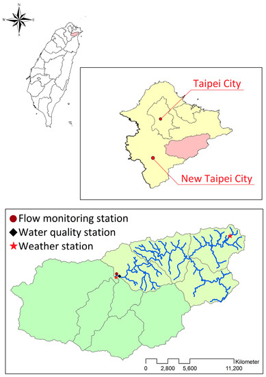
Figure 1.
Location of the Peishi watershed.
2.2. Watershed Models
In this study, we used the HSPF model and SWMM as watershed modeling tools. Both are included in the Better Assessment Science Integrating Point and Nonpoint Sources (BASINS) platform. Multiple GIS data layers are needed to capture land use, watershed boundaries, digital elevation grids, and river systems. After combining the boundary and digital elevation grids, 23 sub-watersheds were automatically defined. These sub-watersheds were used in the HSPF model (Figure 2A) and SWMM (Figure 2B).
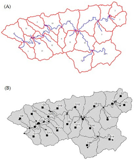
Figure 2.
(A) The sub-watersheds defined by Better Assessment Science Integrating Point and Nonpoint Sources (BASINS) and used in the HSPF model; (B) the same sub-watersheds used in SWMM.
The models require different input data. The HSPF model uses precipitation, evaporation, temperature, wind speed, solar radiation, potential evapotranspiration, dew point temperature, and cloud cover. In contrast, SWMM only uses precipitation, evaporation, temperature, and wind speed. The models also have different requirements for watershed characteristics. The land use data were obtained from the National Land Surveying and Mapping Center in Taiwan. The attributes were recorded in detail according to their geometric space information by aerial photo technology, GIS data, and ground surveys. The HSPF model uses GIS layers to capture the data it needs; for example, it infers hydraulic data from the depth, slope, bottom width of the stream channel, and the flow route. In contrast, SWMM requires pipe characteristics, such as the shape, length, depth, slope, width, and number of junctions. For facile comparison, the delineation of the watershed in SWMM follows the results of the HSPF model, in which 23 subwatersheds were delineated. Table 1 summarizes the model input data for the HSPF model and SWMM.

Table 1.
Summary of the input data for the Hydrological Simulation Program-Fortran (HSPF) model and Storm Water Management Model (SWMM).
Taipei Feitsui Reservoir Administration (TFRA) has implemented monitoring stations in the watershed, including two weather stations, one flow monitoring station, and one water quality monitoring station. The locations of these stations are shown in Figure 1. The rainfall data from the two weather stations were merged with the Thiessen Polygon method, in which the contributing area is divided and used as a weighting factor. The water quality was sampled and analyzed once a month for TP and once a season for SS. The observed data are used to verify the model simulation results.
2.2.1. HSPF Model
The HSPF model can simulate the runoff and NPS pollutant loads that leave a watershed, as well as estimate fate and transport processes in streams and one-dimensional lakes [24]. The HSPF model is an extremely data-intensive and over-parameterized model and requires a large amount of site information to accurately represent hydrology and water quality processes in a watershed [25]. The large number of parameters makes the calibration of distributed watershed models more challenging.
Table 2 defines the important parameters for hydrologic components of the HSPF model that have been discussed in the literature [26,27], including the INFILT (index to infiltration capacity), UZSN (upper zone nominal soil moisture storage), LZSN (lower zone nominal soil moisture storage), IRC (interflow recession), INTFW (interflow inflow), LZETP (lower zone evapotranspiration), AGWRC (fraction of remaining evapotranspiration from active groundwater), and KVARY (variable groundwater recession) parameters. A study by Al-Abed and Whiteley [28] in southern Ontario, Canada showed that LZSN was the most sensitive parameter, followed by the LZSN, PETMAX (temp below which ET is reduced), PACKSNOW (initial quantity of snow), INFILT, and DEEPER (fraction of groundwater inflow to deep recharge) parameters. The PACKSNOW and PETMAX parameters are used when snow is being simulated. Taiwan is located in subtropical and tropical zones. As no snow is in the studied watershed, snow simulation is ignored during modeling.

Table 2.
Important parameters for the hydrologic components of the HSPF model.
In this case, the suspended solid (SS) and total phosphorous (TP) concentrations are of concern. From the literature [29,30], JRER (exponent in the soil detachment equation), JSER (exponent in the sediment wash-off equation), and JGER (exponent in soil matrix scour equation) are sensitive parameters for SS simulation. For phosphorous modeling, the method used assumes a first-order kinetics equation to represent each of the soil phosphorous processes. Each equation contains two parameters, the kinetics rate, which is calibrated manually, and the temperature coefficient, which is maintained at a specified value [31].
2.2.2. SWMM
SWMM is a dynamic hydrologic-hydraulic water quality simulation model that is primarily used for urban areas; however, it also has applications for drainage systems in non-urban areas [12,13]. The model conceptualizes a drainage system as a series of water and material flows between several environmental compartments. The runoff is calculated by approximating a non-linear reservoir model, considering depression loss, infiltration, evaporation, and storage. SWMM offers three methods to simulate how rainfall infiltrates into the upper soil zone in a sub-catchment: Horton infiltration, Green-Ampt infiltration, and Curve Number infiltration. Table 3 shows the important parameters for the hydrologic components of SWMM. In this study, the version we used is SWMM 5.0, which can be downloaded freely from the US EPA website.

Table 3.
Important parameters for the hydrologic components of SWMM.
Because forests are the major land cover in the study area, perviousness is a more important factor than imperviousness. Six parameters were chosen for sensitivity analysis: width, N-Perv (Manning’s roughness coefficient for pervious and impervious areas), and I-Max (maximum infiltration rate) for the Horton infiltration method, and Cond (saturated hydraulic conductivity), D-Ini (initial moisture deficit), and SucH (suction head at the wetting front) for the Green-Ampt infiltration method.
SWMM uses build-up and wash-off functions for simulating water quality. In this study, a power function is used for the build-up function, and the event mean concentration is used for the wash-off function. When simulating water quality, the user chooses one of the build-up and wash-off functions and determines the parameter values with a calibration and validation process. These parameter values will be different for different pollutants and land uses.
2.3. Parameter Sensitivity Analysis
SA can identify the most influential parameters and assess which parameters contribute most to the variability in the output. A one-factor-at-a-time (OAT) approach can be used to determine the sensitivity of an individual parameter by repeatedly varying that parameter and calculating the resulting changes in output while holding all of the other model parameters constant. However, accurate output distribution results depend on a complete sampling of input distributions; that is, the sampling must guarantee full coverage of the parameter space.
Latin Hypercube (LH) sampling is a stratification of the input probability distributions. Stratification divides the cumulative curve into equal intervals on the cumulative probability scale (0 to 1). A sample is randomly taken from each interval or “stratification” of the input distribution (Figure 3). The LH method ensures that sample values more accurately reflect the input probability distribution. As a more efficient sampling method, LH offers great benefits in terms of increased sampling efficiency and faster runtimes (due to fewer iterations). All parameters are assumed to follow a normal distribution, and the probability distributions are expressed in cumulative form. The input ranges of each parameter are assigned based on technical notes and previous literature. The initial parameters are the results of previous model validation. LH sampling is a sophisticated way to perform random sampling and provides robust and effective results [18].
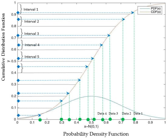
Figure 3.
Illustration of the Latin Hypercube (LH) sampling process. The user decides the number of intervals to divide the distributions, and a sample is taken randomly from each interval.
Therefore, we used the LH-OAT method, which combines OAT design and LH sampling by taking the LH samples as initial points in the OAT approach [20]. For a model with N total parameters, LH-OAT divides each parameter into K intervals and generates K LH sample points. Each one of the K LH samples is altered N times, changing only one of the N parameters at a time. For an LH sample point m, a partial sensitivity index can be calculated as the variance for each parameter , as follows [15,22]:
where O is the sum of the square of errors between the simulated and the observed output, fi is the fraction by which parameter Pi is changed and j is the LH point. Each sample point requires N + 1 model runs. In this study, we evaluated 15 hydrology parameters for the HSPF model and 6 parameters for SWMM; each parameter was divided into 20 intervals for the LH-OAT method. The final sensitivity index was calculated for each parameter by averaging the partial indices shown in Equation (1).
3. Results and Discussion
3.1. Model Performance Evaluation
3.1.1. Simulation of Daily Flow
The observed flow data included continuous daily flow measurements, and the observed water quality data consisted of monthly monitoring data. The water quality was sampled and analyzed once a month and once a season for TP and SS, respectively. The data from 2008 to 2010 were used for model calibration to identify adequate model parameters, and the data from 2011 to 2012 were used for model validation to verify the feasibility of the model parameters. Flow calibration and validation are required for using a water quality model. During the calibration process, the sensitive parameters were changed iteratively, and a statistical method was used to find an acceptable fit to the observed data. Figure 4 and Figure 5 shows the flow simulation results from both models.
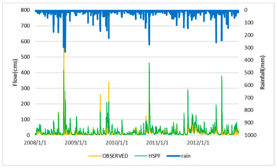
Figure 4.
Flow simulation results for the HSPF model.
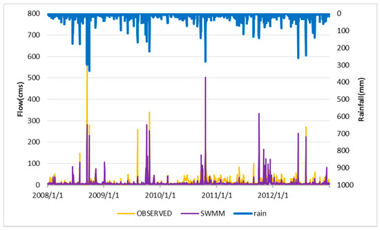
Figure 5.
Flow simulation results for the SWMM model.
We used two statistical methods to evaluate the goodness-of-fit of each model’s flow simulation: the correlation coefficient (r), the coefficient of determination (R2). The values of r and R2 range from 0 to 1, with higher values indicating better agreement between the modeled and observed data.
Table 4 shows the results of the model fitness analysis for daily flow. In the HSPF model, the r and R2 values obtained from the calibration tests were 0.78 and 0.61, respectively. According to the performance rating by Donigian [26], r ≥ 0.85 or R2 ≥ 0.7 indicates good model performance. For the HSPF validation, the r and R2 values obtained were 0.86 and 0.74, respectively. In SWMM, the r and R2 values obtained from the calibration tests were 0.84 and 0.71, respectively, and were 0.78 and 0.62 for the validation period. These results suggest good performance for both models. The flow simulations of both models were satisfactory.

Table 4.
Results of the model fitness analysis for daily flow.
3.1.2. Simulation of the Water Quality
After the flow simulations were shown to be acceptable, water quality simulations were performed, and the model parameters related to flow were held constant. Figure 6 and Figure 7 show the SS and TP simulation results for both models. Unlike the 365 daily flow data measurements, only 4 water quality measurements were taken each year for SS and 12 each year for TP. Therefore, we used the mean percentage error (MPE) to evaluate the TP and SS results. Table 5 summarizes the calibration and validation of water quality for both models. For the SS simulation, the MPE values for calibration and validation were 35.3% and 38.9% in the HSPF model, and were 28.3% and 36.3% in SWMM. For the TP simulation, these values were 34.3% and 30.1% in the HSPF model and 33.5% and 36.1% in SWMM.
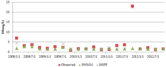
Figure 6.
Validation of the SS simulation for the HSPF model and SWMM.
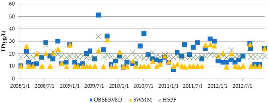
Figure 7.
Validation of the TP simulation for the HSPF model and SWMM.

Table 5.
Results of the model fitness analysis for suspended solid (SS) and total phosphorous (TP).
3.2. Sensitivity Analysis for the Hydrology Simulation
Table 6 and Table 7 give the final sensitivity index of each chosen parameter obtained from the HSPF model and SWMM. A larger sensitivity index indicates that a parameter has a greater influence on the simulated flow output.

Table 6.
Sensitivity index values for parameters from the HSPF model.

Table 7.
Sensitivity index values for parameters from SWMM.
For the HSPF model, the five most sensitive hydrologic parameters were UZSN, INFILT, LZSN, NSUR, and SLSUR. The UZSN, INFILT, and LZSN parameters have much stronger effects than the other parameters. The UZSN and LZSN parameters reflect the upper and lower zone nominal soil moisture storage, respectively. The LZSN parameter is related to both precipitation patterns and soil characteristics, and the UZSN parameter is related to land surface characteristics and topography. The INFILT parameter is an index of the mean soil infiltration rate and controls the division of the available moisture from precipitation into surface and subsurface flow and storage components in the HSPF model. When the value of INFILT increases, more water enters the lower zone and groundwater and the infiltration volume increases. Low INFILT values produce more upper zone and interflow storage and result in high direct surface flow.
Sensitivity analysis on the HSPF model has been performed in many previous studies (e.g., Jacomino and Fields, 1997; Fonseca et al., 2014) [34,35]. However, due to the use of different values of the HSPF model parameters, the major factors affecting model output for each watershed may be different. Al-Abed and Whiteley [28] and Fonseca et al. [35] found that LZSN is the major factor, INFILT is the most sensitive parameter in a complex geomorphological river basin (Kourgialas et al. [36]) and in the South National watershed in Eastern Ontario (Iskra and Droste, [37]), and DEEPFR is the most sensitive parameter in mountainous basins containing coal mines (Atkins et al. [38]). However, we found that UZSN and INFILT are more sensitive. The main reason for this difference is that the studied watershed is located in a subtropical area and experiences no snow effects.
For SWMM, the sensitivity index values of Manning’s roughness coefficient for pervious areas and the width were 22.0 and 21.9, respectively; these results indicate that these parameters have a similar effect on the flow simulation. In the Horton infiltration method, the value of the sensitivity index for the maximum infiltration rate was 0.1. When compared with the Manning’s roughness coefficient and the width, the maximum infiltration rate is a less sensitive parameter. This result is consistent with the results of Li et al. [17], who also used the Horton infiltration method; they found that in a sub-catchment area, the width and Manning’s roughness coefficient for pervious and impervious areas had a greater effect on the total runoff volume than the maximum infiltration rate. A study in the Ballona Creek Watershed in Southern California showed that total runoff and peak flow were most strongly affected by imperviousness and impervious depression storage; surface flow was least sensitive to Manning’s roughness coefficient [32]. Manning’s roughness coefficient for the conduit had the highest influence on the total runoff volume [17].
Sensitivity analysis was also applied to the Green-Ampt infiltration method in SWMM. For this method, the infiltration, conductivity, and initial deficit parameters were much more sensitive than Manning’s roughness coefficient for pervious areas and the width. The hydraulic conductivity of soil depends on the soil characteristics. The sensitivity index for the soil hydraulic conductivity was the largest in this study.
In general, the parameters related to infiltration and soil characteristics have a relatively large effect on the flow simulation in both models, except when using the Horton infiltration method in SWMM. The Manning’s roughness coefficient for pervious areas was much more sensitive in SWMM than in the HSPF model. This difference can be explained by the calculations in each model. The HSPF model uses the Chezy-Manning equation to calculate runoff, as well as several empirical equations. In contrast, a nonlinear storage equation is used in SWMM.
3.3. Comparison of the Model Simulation Results
Table 8 compares the daily flow simulated by both models to observations from 2007 to 2012. Although statistical analyses suggests that both models simulated daily flow well, there are clear differences between the simulated results from each model and observations. The observed average daily flow was 12.9–18.8 m3/s. The average daily flow simulated by the HSPF model exceeded these values, ranging from 25.3 to 31.4 m3/s. In contrast, the average daily flow simulated by SWMM was lower than the observations, ranging from 8.4 to 11.2 m3/s. This difference is related to the calculations in each model. The HSPF model uses complex calculations for the various soil layers of pervious areas to simulate flow, while SWMM only has one infiltration function for pervious areas and a constant dry weather flow as groundwater. Therefore, for SWMM, the model parameters involved in the infiltration function control the simulated flow for pervious areas. For the minimum daily flow, the results simulated by the HSPF model were close to the observed values; however, the SWMM results were fixed at 4 m3/s, which is the input base flow.

Table 8.
Comparison between daily flows simulated by the HSPF model and SWMM and observed data (m3/s).
Both models could capture high flow values during peak flow simulations. Peak flows result from high precipitation. However, the model performance for each storm event was different. The peak flows in the SWMM simulations were generally higher than the peak flows in the HSPF simulations; recession was quicker in the SWMM simulations than in the HSPF simulations. These differences meant that SWMM simulated lower flows following a heavy storm event than both the HSPF model and the observations. This difference was apparent in each simulated year, including the events on 21 October 2010, 3 October 2011, and 2 August 2012 (Figure 8). The quick recession in the SWMM simulations might be caused by the infiltration calculation and constant groundwater assumption. If the groundwater behavior is considered, the recession might be extended. However, there were fewer differences between small storm events. For small storms, the HSPF model simulated slightly higher flows than the observations, and the SWMM simulated flows were slightly lower than the observations. These results suggest that the NPS loadings could be underestimated by SWMM in small storm events.
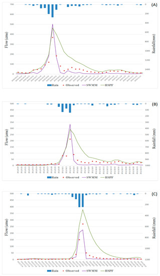
Figure 8.
Daily flow simulation results for both models and observations during storm events on (A) 21 October 2010; (B) 3 October 2011; and, (C) 2 August 2012.
Figure 9 and Figure 10 compare the SS and TP values simulated by the two models with observations. The maximum SS concentration was 286.0 mg/L in the HSPF model but only 4.3 mg/L in SWMM. The SS concentrations simulated by the HSPF model were closely linked to precipitation. In contrast, the SS concentrations did not vary significantly with precipitation in SWMM. This difference could be derived from the effects of wash-off and build-up on the maximum pollutant load in both models. However, the SWMM simulations of SS achieved a slightly better validation result than the HSPF simulations, mainly because no samples were collected during storm events. Rather, samples were most often collected on sunny days, and thus, the observations do not reflect the SS concentration during intense precipitation events.
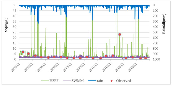
Figure 9.
SS concentrations obtained from the HSPF and SWMM simulations and observations.
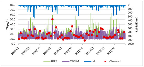
Figure 10.
TP concentrations obtained from the HSPF and SWMM simulations and observations.
The maximum observed TP concentration during the study period was 0.051 mg/L; the maximum simulated TP concentrations were 0.097 and 0.047 mg/L for the HSPF model and SWMM, respectively. This difference between the observed and simulated TP concentrations is small when compared to the SS data.
We note that there are significant differences in the TP and SS trends simulated by the HSPF model and SWMM. In the HSPF model, pollutants are produced with rainfall and are affected by hydrologic routes; thus, the trend in simulated water quality follows rainfall. However, the SWMM uses build-up and wash-off functions to simulate water quality rather than considering pollutant transport and distribution. Pollutant build-up is a function of the number of preceding dry weather days; pollutant wash-off occurs during wet weather, at which time runoff is calculated as a function of the amount of buildup. While the HSPF model simulates the pollutants lost from the surface to groundwater flow within a watershed, the simulation of pollutants in the HSPF model is extremely sensitive to hydrology, particularly the amount and timing of surface runoff. Basically, pollutants are produced with rainfall, and their distribution is affected by hydrologic routes in the HSPF model, while SWMM considers pollutants that accumulate before rainfall and then wash out with the runoff. Finally, there is a lag between the results of the HSPF model and SWMM: the peak TP and SS concentrations occur at different times. SWMM is usually applied in urban areas rather than upstream watersheds, like the study area where permeable land is prevalent. In the study area, the HSPF simulations followed precipitation; the HSPF simulation of NPS pollution seems to be more consistent with observations than the SWMM simulation.
4. Conclusions
In this study, the HSPF and SWMM watershed models were used to simulate NPS pollution in a watershed where 93% of the land cover is forest. Both of the models are acceptable according to statistical analysis, but their simulation performances are different because of their underlying calculation mechanisms. The average daily flow was higher than observations in the HSPF simulations and lower in the SWMM simulations. Recession occurred more rapidly in the SWMM simulations because the model only considers surface infiltration in underground flow routes. In the HSPF model, underground flow routes in pervious areas are more complex, resulting in a slow recession flow curve that more closely resembles observations. Both of the models can simulate continuous SS and TP concentrations with acceptable goodness-of-fit results. However, the SS concentrations simulated by the HSPF model were consistent with precipitation, while the SS concentrations simulated by SWMM were not. In the HSPF model, once pollutants are generated, they are transported along flow routes, but pollutants in SWMM are controlled by build-up and wash-off functions. There is a clear lag time between peak pollutant concentrations in the HSPF model and SWMM.
In the HSPF model, the UZSN, INFILT, LZSN, NSUR, and SLSUR parameters were the five most sensitive hydrologic parameters. The UZSN, INFILT, and LZSN parameters had the greatest effects on the model output. These parameters relate to the infiltration function, precipitation patterns, and soil and land surface characteristics. This result differs from the results of a previous study (AL-Abed and Whiteley et al., 2002) that examined a watershed with a polar climate. In that study, the authors found that LZSN was the most sensitive parameter, followed by the snow-related parameters. For SWMM, the conductivity and the initial deficit in the infiltration calculations were more sensitive than the geometric characteristics (width) and Manning’s roughness coefficient for pervious areas. The sensitivity analysis results show that the parameters related to soil characteristics have the greatest influence on the stream flow simulation in both of the models.
SWMM is usually applied in urban watersheds rather than forested upstream watersheds, such as the study area. However, our results show that the SWMM simulations are comparable to those of the HSPF model, suggesting that both models can be applied in these watersheds. However, users should be aware that in highly pervious areas, SWMM might underestimate the daily flow and pollutant concentrations for small storm events.
Author Contributions
All authors were involved in designing and discussing the study. Lin-Yi Tsai drafted and finalized the manuscript. Chi-Feng Chen and Chi-Hsuan Fan collected the required data and executed the model. Jen-Yang Lin coordinated the group and revised the manuscript. All authors have read and approved the final manuscript.
Conflicts of Interest
The authors declare no conflict of interest.
References
- Yang, Y.S.; Wang, L. A review of modeling tools for implementation of the EU water framework directive in handling diffuse water pollution. Water Resour. 2010, 24, 1819–1843. [Google Scholar]
- Nasr, A.; Bruen, M.; Jordan, P.; Moles, R.; Kiely, G.; Byrne, P. A comparison of SWAT, HSPF and SHETRAN/GOPC for modeling phosphorus export from three catchments in Ireland. Water Res. 2007, 41, 1065–1073. [Google Scholar] [CrossRef] [PubMed]
- Xu, Z.; Godrej, A.N.; Grizzard, T.J. The hydrological calibration and validation of a complexly-linked watershed–reservoir model for the Occoquan watershed, Virginia. J. Hydrol. 2007, 345, 167–183. [Google Scholar] [CrossRef]
- Choi, W.; Deal, B.M. Assessing hydrological impact of potential land use change through hydrological and land use change modeling for the Kishwaukee River basin (USA). J. Environ. Manag. 2008, 88, 1119–1130. [Google Scholar] [CrossRef] [PubMed]
- Hunter, H.M.; Walton, R.S. Land-use effects on fluxes of suspended sediment, nitrogen and phosphorus from a river catchment of the Great Barrier Reef, Australia. J. Hydrol. 2008, 356, 131–146. [Google Scholar] [CrossRef]
- Chung, E.S.; Lee, K.S. Prioritization of water anagement for sustainability using hydrologic simulation model and multicriteria decision making techniques. J. Environ. Manag. 2009, 90, 1502–1511. [Google Scholar] [CrossRef] [PubMed]
- Campbell, C.W.; Sullivan, S.M. Simulating time-varying cave flow and water levels using the Storm Water Management Model. Eng. Geol. 2002, 65, 133–139. [Google Scholar] [CrossRef]
- Jang, S.; Cho, M.; Yoon, J.; Yoon, Y.; Kim, S.; Kim, G.; Kim, L.; Aksoy, H. Using SWMM as a tool for hydrologic impact assessment. Desalination 2007, 212, 344–356. [Google Scholar] [CrossRef]
- Temprano, J.; Arango, Ó.; Cagiao, J.; Suárez, J.; Tejero, I. Stormwater quality calibration by SWMM: A case study in Northern Spain. Water SA 2005, 32, 55–63. [Google Scholar] [CrossRef]
- Di Modugno, M.; Gioia, A.; Gorgoglione, A.; Iacobellis, V.; la Forgia, G.; Piccinni, A.F.; Ranieri, E. Build-up/Wash-Off Monitoring and Assessment for Sustainable Management of First Flush in an Urban Area. Sustainability 2015, 7, 5050–5070. [Google Scholar] [CrossRef]
- Pretorius, H.; James, W.; Smit, J. A Strategy for Managing Deficiencies of SWMM Modeling for Large Undeveloped Semi-Arid Watersheds. J. Water Manag. Model. 2013, R246–R301. [Google Scholar] [CrossRef]
- Moynihan, K.; Vasconcelos, J. SWMM Modeling of a Rural Watershed in the Lower Coastal Plains of the United States. J. Water Manag. Model. 2014. [Google Scholar] [CrossRef]
- Talbot, M.; McGuire, O.; Olivier, C.; Flemin, R. Parameterization and application of agricultural best management practices in a rural Ontario watershed using PCSWMM. J. Water Manag. Model. 2016. [Google Scholar] [CrossRef]
- Chen, C.F.; Tsai, L.I.; Fan, C.H.; Lin, J.Y. Using Exceedance Probability to Determine Total Maximum Daily Loads for Reservoir Water Quality Management. Water 2016, 8, 541. [Google Scholar] [CrossRef]
- Muleta, M.K. Comparison of Model Evaluation Methods to Develop a Comprehensive Watershed Simulation Model. In Proceedings of the 2010 Conference of the Environmental and Water Resources Institute, Palm Springs, CA, USA, 16 May 2010; pp. 2492–2501. [Google Scholar]
- Jakeman, A.J.; Letcher, R.A.; Norton, J.P. Ten iterative steps in development and evaluation of environmental models. Environ. Model. Softw. 2006, 21, 602–614. [Google Scholar] [CrossRef]
- Li, C.; Wang, W.; Xiong, J.; Chen, P. Sensitivity Analysis for Urban Drainage Modeling Using Mutual Information. Entropy 2014, 16, 5738–5752. [Google Scholar] [CrossRef]
- Saltelli, A. What is sensitivity analysis? In Sensitivity Analysis; Saltelli, A., Chan, K., Scott, E.M., Eds.; Wiley: New York, NY, USA, 2000. [Google Scholar]
- Morris, M.D. Fractional sampling plants for preliminary computational experiments. Technometrics 1991, 33, 161–174. [Google Scholar] [CrossRef]
- Van Griensven, A.; Meixner, T.; Grunwald, S.; Bishop, T.; Diluzio, A.; Srinivasan, R. A global sensitivity analysis tool for the parameters of multi-variable catchment models. J. Hydrol. 2006, 324, 10–23. [Google Scholar] [CrossRef]
- Helton, J.C.; Davis, F.J. Illustration of sampling-based methods for uncertainty and sensitivity analysis. Risk Anal. 2002, 22, 591–622. [Google Scholar] [CrossRef] [PubMed]
- Nossent, J.; Bauwens, W. Multi-variable sensitivity and identifiability analysis for a complex environmental model in view of integrated water quantity and water quality modeling. Water Sci. Technol. 2012, 65, 539–549. [Google Scholar] [CrossRef] [PubMed]
- Holvoet, K.; van Griensven, A.; Seuntjens, P.; Vanrolleghem, P.A. Sensitivity analysis for hydrology and pesticide supply towards the river in SWAT. Phys. Chem. Earth 2005, 30, 518–526. [Google Scholar] [CrossRef]
- Bicknell, B.R.; Imhoff, J.C.; Kittle, J.L.; Donigian, A.S.; Johanson, R.C. Hydrological Simulation Program—FORTRAN; User’s Manual for Version 11; Rep. No. EPA/600/R-97/080; U.S. EPA: Athens, Greece, 1997.
- Im, S.J.; Brannan, K.M.; Mostaghimi, S.; Kim, S.M. Comparison of HSPF and SWAT models performance for runoff and sediment yield prediction. J. Environ. Sci. Health Toxic Hazard Subst. Environ. Eng. 2007, 42, 1561–1570. [Google Scholar] [CrossRef] [PubMed]
- Donigian, A.J. Watershed model calibration and validation: The HSPF experience. Proc. Water Environ. Fed. 2002, 8, 44–73. [Google Scholar] [CrossRef]
- Seong, C.; Her, Y.; Benham, B.L. Automatic Calibration Tool for Hydrologic Simulation Program-FORTRAN Using a Shuffled Complex Evolution Algorithm. Water 2015, 7, 503–527. [Google Scholar] [CrossRef]
- Al-Abed, N.A.; Whiteley, H.R. Calibration of the Hydrological Simulation Program Fortran (HSPF) Model Using Automatic Calibration and Geographical Information Systems. Hydrol. Process. 2002, 16, 3169–3188. [Google Scholar] [CrossRef]
- Hayashi, S.; Murakami, S.; Watanabe, M.; Xu, B.H. HSPF Simulation of Runoff and Sediment Loads in the Upper Changjiang River Basin, China. J. Environ. Eng. 2004, 130, 801–815. [Google Scholar] [CrossRef]
- Fontaine, T.A.; Jacomino, M.F. Sensitivity analysis of simulated contaminated sediment transport. J. Am. Water Resour. Assoc. 1997, 33, 313–325. [Google Scholar] [CrossRef]
- U.S. Environmental Protection Agency. In Environmental Protection Agency. Estimating Hydrology and Hydraulic Parameters for HSPF: EPA BASINS Technical; Note 6; Office of Water: Washington, DC, USA, 2000.
- Barco, J.; Wong, K.M.; Michael, K.; Stenstrom, F. Automatic Calibration of the U.S. EPA SWMM Model for a Large Urban Catchment. J. Hydraul. Eng. 2008, 34, 466–474. [Google Scholar] [CrossRef]
- Beling, F.A.; Garcia, J.I.B.; Paiva, E.M.C.D.; Bastos, G.A.P.; Paiva, J.B.D. Analysis of the SWMM Model Parameters for Runoff Evaluation in Periurban Basins from Southern Brazil. In Proceedings of the 12nd International Conference on Urban Drainage, Porto Alegre, Brazil, 11–16 September 2011. [Google Scholar]
- Jacomino, V.M.F.; Fields, D.E. A critical approach to the calibration of a watershed model. J. Am. Water Resour. Assoc. 1997, 33, 143–154. [Google Scholar] [CrossRef]
- Fonseca, A. Watershed model parameter estimation and uncertainty in data-limited environments. Environ. Model. Softw. 2014, 51, 84–93. [Google Scholar] [CrossRef]
- Kourgialas, N.N.; Karatzas, G.P.; Nikolaidi, N.P. An integrated framework for the hydrologic simulation of a complex geomorphological river basin. J. Hydrol. 2010, 381, 308–321. [Google Scholar] [CrossRef]
- Iskra, I.; Droste, R. Parameter uncertainty of a watershed model. Can. Water Resour. J. 2008, 33, 5–22. [Google Scholar] [CrossRef]
- Atkins, J.T., Jr.; Wiley, J.B.; Paybins, K.S. Calibration Parameters Used to Simulate Streamflow from Application of the Hydrologic Simulation Program FORTRAN Model (HSPF) to Mountainous Basins Containing Coal Mines in West Virginia; Scientific Investigations Report 2005-5099; USGS: Reston, VA, USA, 2005.
© 2017 by the authors. Licensee MDPI, Basel, Switzerland. This article is an open access article distributed under the terms and conditions of the Creative Commons Attribution (CC BY) license (http://creativecommons.org/licenses/by/4.0/).