Optimal Temporal Resolution of Rainfall for Urban Applications and Uncertainty Propagation

Abstract

The optimal temporal resolution for rainfall applications in urban hydrological models depends on different factors. Accumulations are often used to reduce uncertainty, while a sufficiently fine resolution is needed to capture the variability of the urban hydrological processes. Merging radar and rain gauge rainfall is recognized to improve the estimation accuracy. This work explores the possibility to merge radar and rain gauge rainfall at coarser temporal resolutions to reduce uncertainty, and to downscale the results. A case study in the UK is used to cross-validate the methodology. Rainfall estimates merged and downscaled at different resolutions are compared. As expected, coarser resolutions tend to reduce uncertainty in terms of rainfall estimation. Additionally, an example of urban application in Twenterand, the Netherlands, is presented. The rainfall data from four rain gauge networks are merged with radar composites and used in an InfoWorks model reproducing the urban drainage system of Vroomshoop, a village in Twenterand. Fourteen combinations of accumulation and downscaling resolutions are tested in the InfoWorks model and the optimal is selected comparing the results to water level observations. The uncertainty is propagated in the InfoWorks model with ensembles. The results show that the uncertainty estimated by the ensemble spread is proportional to the rainfall intensity and dependent on the relative position between rainfall cells and measurement points.

1. Introduction

The problem of the optimal spatial and temporal resolution for rainfall estimates in urban hydrology applications has been widely debated. On the one hand, many studies analyse the ideal resolution for model application. The optimal temporal and spatial resolutions for urban hydrology is studied by Schilling [1] as a function of hydrologic parameters of the catchment. In the work of Berne et al. [2], equations are derived to calculate the optimal spatial and temporal resolutions, given the area of a catchment, and they recommend 5 min–3 km for catchments of 1000 ha and 3 min–2 km for catchments of 100 ha. Gabellani et al. [3] suggest that a temporal resolution equal to 0.2 the characteristic catchment time and a spatial resolution of 0.2 the characteristic catchment dimension are the minimum requirements to avoid major errors in runoff estimation. Nevertheless, models have drastically evolved in the last 20 years and the concept of optimal resolution with them. Thanks to the increased computation capabilities, models are more complex and can represent finer scale phenomena, especially in the urban environment. There is a trend of moving towards integrated models, able to predict both the water quality and quantity, representing urban drainage networks, surface runoff processes, river hydraulics, chemical dynamics, wastewater treatment plants, and so on [4]. At the same time, rainfall measurements have improved with the use of weather radars, which are able to achieve a finer spatial resolution and improved the accuracy thanks to technological advancements such as the use of dual polarization and Doppler capabilities [5,6]. Today, weather radars can provide rainfall estimates at 5-min/1 km resolutions, although they still present a lower accuracy compared to point measurements, due to the indirect nature of the radar rainfall estimation [7,8]. Radar data at fine temporal resolution can present temporal sampling errors, which can be reduced with accumulation or with advanced storm advection techniques [9,10,11]. Merging radar and rain gauge rainfall information is recognized to improve the radar rainfall estimation accuracy, maintaining the radar spatial resolution characteristics [12,13,14,15,16] and the accuracy of the point rain gauge measurements. Among the most popular techniques, Kriging with External Drift (KED) and Conditional Merging (CM) proved to achieve a good performance [12,14,17,18]. Although KED has the advantage of providing a strong platform for uncertainty estimation, thanks to the easily derivable kriging variance, it may not perform comparably well at short temporal resolutions, which are often necessary for urban hydrological applications [19]. In particular, KED is very sensitive to low quality data at fine temporal resolutions [19]. A possible approach is to improve robustness of KED using a co-kriging with external drift approach, or an extensive data pre-processing to achieve a sufficient data quality [20,21].

This work aims at exploring the possibility of using KED at a coarser temporal resolution, in order to improve the result stability and reduce the impact of random errors, and subsequently downscale the results. By downscaling both the KED estimation and the associated variance, the rainfall uncertainty can be studied and propagated in urban hydrological models. Most of the downscaling techniques discussed in the literature are stochastic [22,23,24,25], usually used to explore climatic variability. Instead, in this work, we use a data-driven approach, based on the radar data available at 5-min resolution to downscale the KED estimates and variance. The aim of this approach is to study the uncertainty associated with the rainfall data, rather than the process variability.

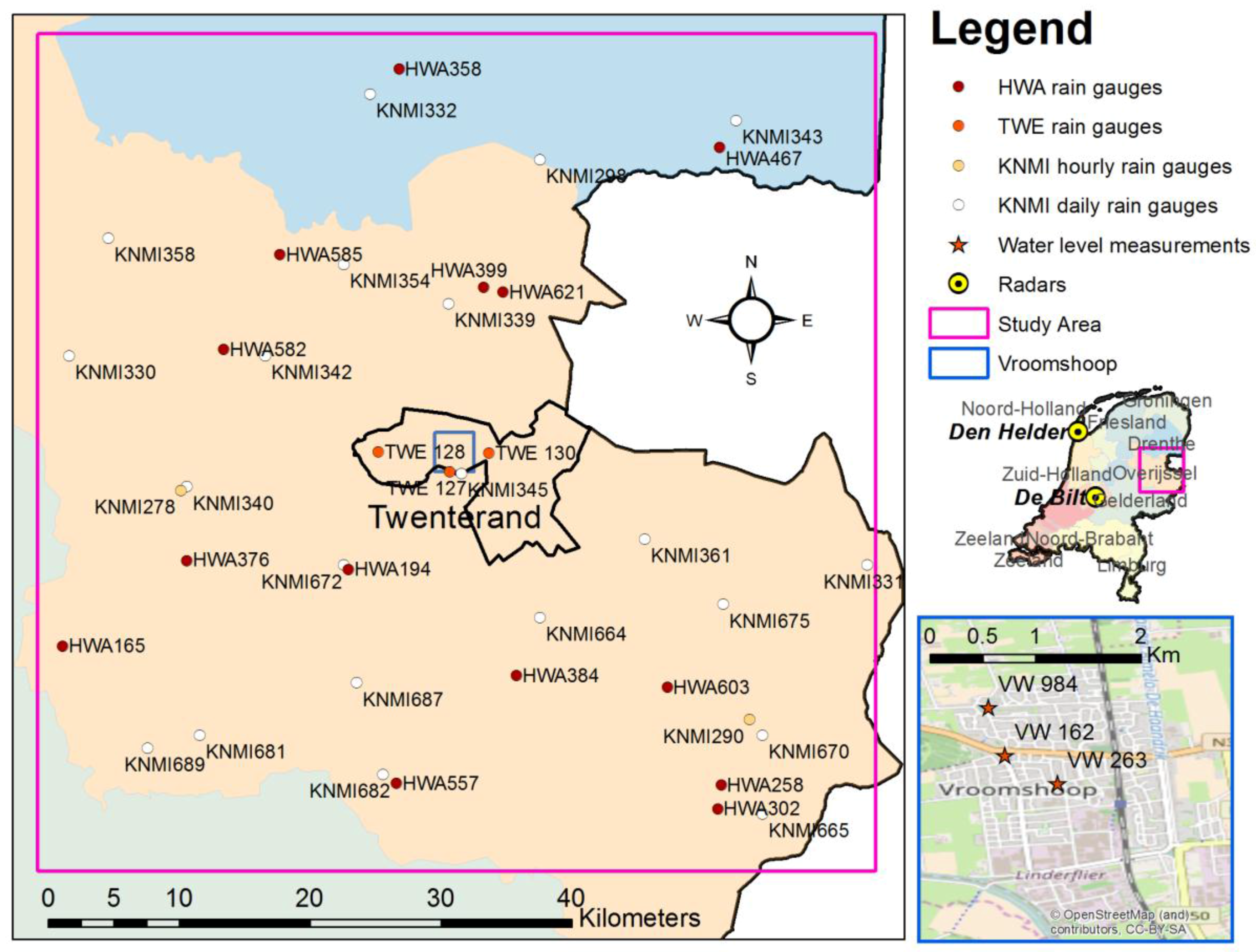
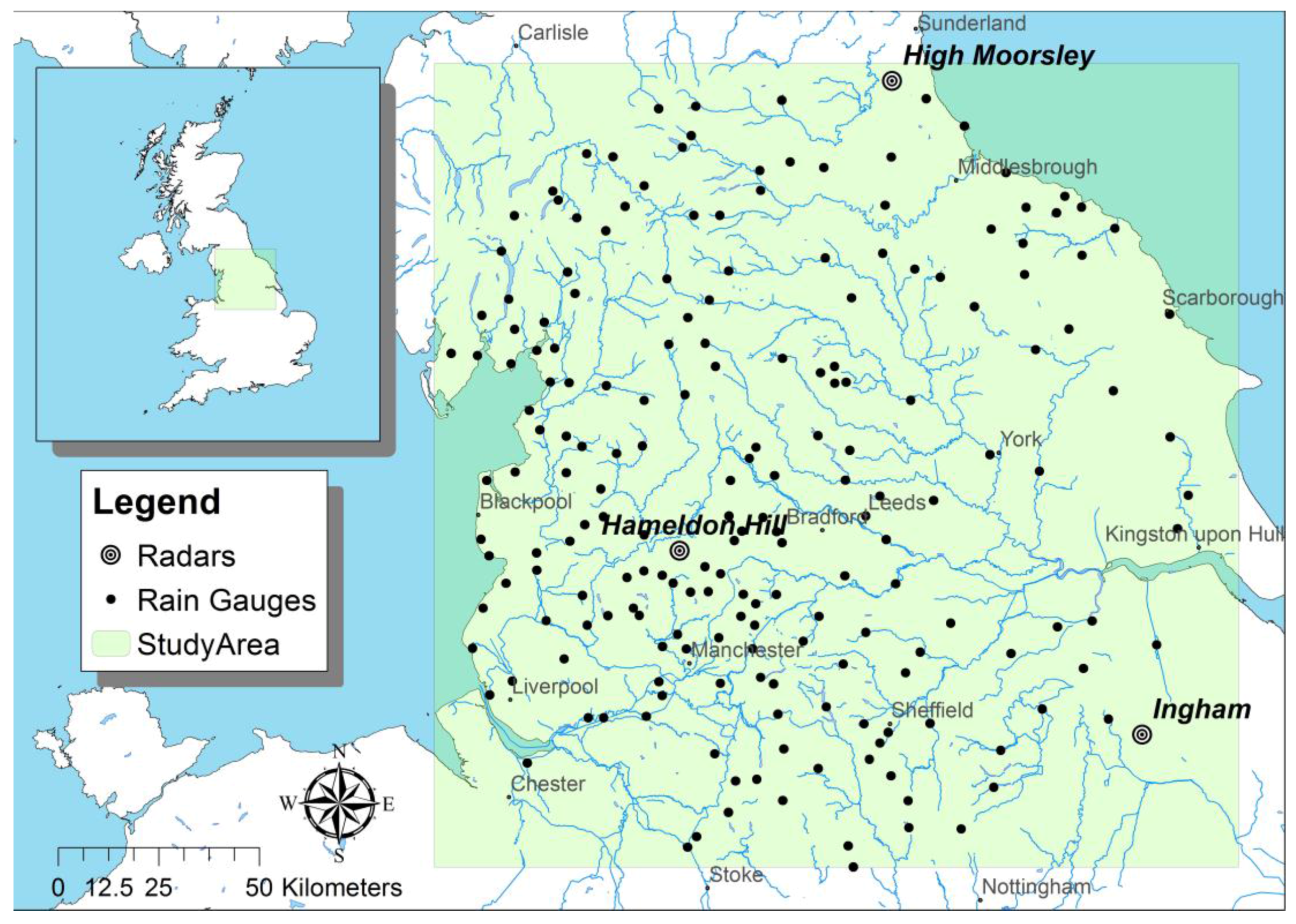
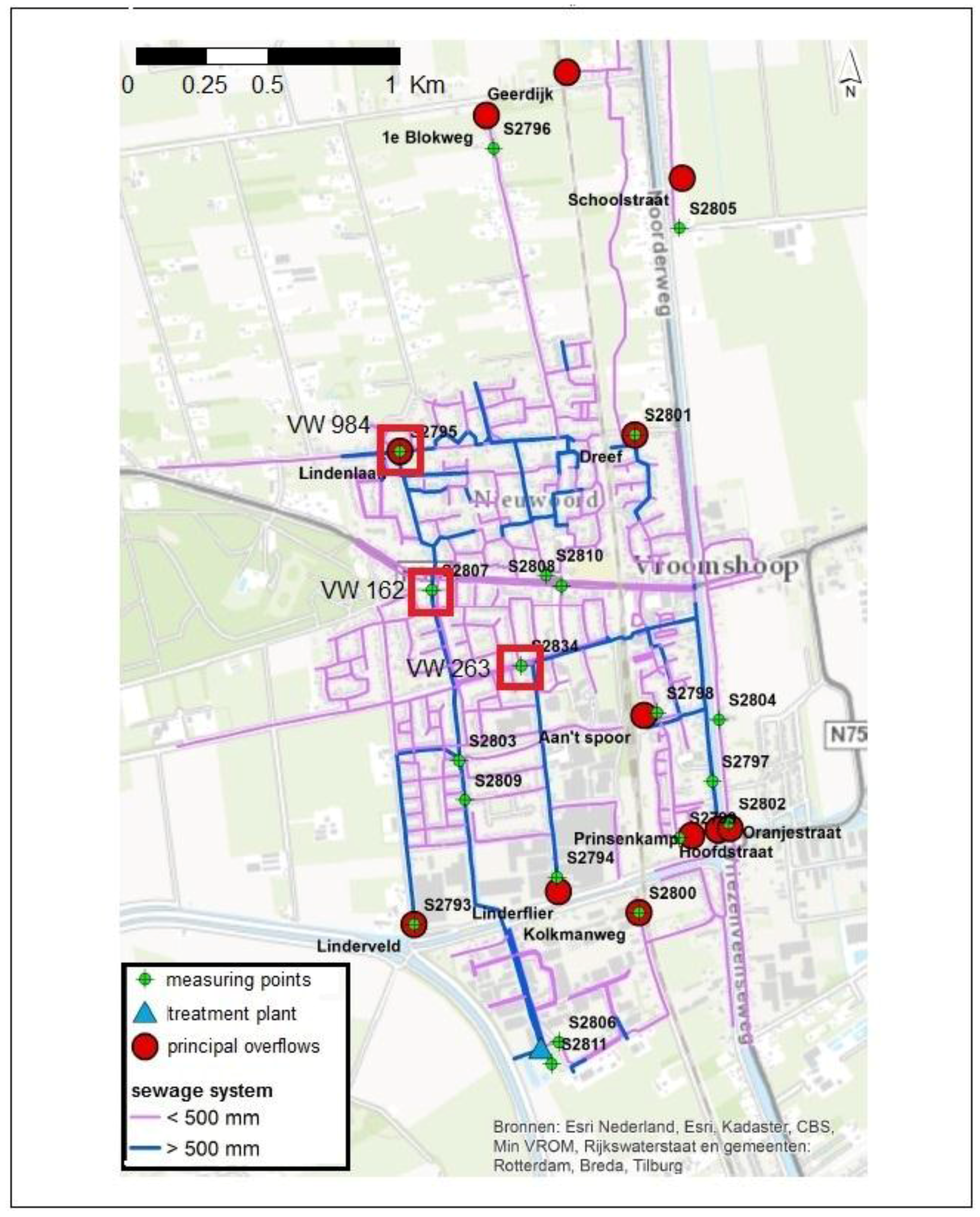
A case study with about 200 rain gauges and radar composites from 3 C-band radars, in an area of about 200 by 200 km² in England is used to perform cross-validation and verify the methodology. Twelve combinations of different accumulation and downscaling resolutions are tested. Additionally, an example of application to urban modelling is presented. The optimal accumulation and downscaling resolutions for a specific model are identified by comparing different products with 14 combinations of accumulation resolutions and downscaling resolutions in a case study in the Netherlands. The generated rainfall products are tested, using an InfoWorks urban hydrological model. The case study is based on a high-intensity convective rainfall event that occurred in the Municipality of Twenterand, in the east of the Netherlands, causing severe flooding in the village of Vroomshoop. The InfoWorks model of the Vroomshoop area and water level measurements are used to identify the optimal combination of accumulation and downscaling resolutions for the specific model, by comparing the deterministic KED predictions. For the selected product, the uncertainty propagation is studied, producing an ensemble from the probabilistic KED result and using it in the InfoWorks model.

In Section 2, the case studies are described, presenting the datasets and the model. In Section 3, the methods used to compare the accumulation and downscaling times, to merge radar and rain gauge data, to downscale the merged products, and to produce the ensemble are presented. Section 4 and Section 5 present and discuss the results respectively. Section 6 summarizes the conclusions and recommendations.

2. Dataset and Model

2.1. Case Study 1: United Kingdom

The objective of the proposed methodology is to optimize rainfall for an urban model application. The case study in Twenterand, Overijssel, The Netherlands, is used for this purpose, thanks to the available InfoWorks model. However, a validation of the used techniques, in terms of rainfall reproduction capabilities, needs to be performed. The case study in the Netherlands cannot be used for this purpose, because the number of available rain gauges that could be used as a reference is limited, and their accuracy and temporal resolution are highly variable. For this reason, we use a different dataset to evaluate how the proposed approach performs in terms of rainfall prediction. A case study in the northern part of England is considered. The same methodology applied to the Dutch case study is applied to the UK case study, but instead of using the products in a model, the rainfall products are validated through cross-validation. For the test, we consider six months of data, between 1 January 2016 at 00:00 UTC and 30 June 2016 23:59 UTC, considering only the hourly time steps in which at least a rain gauge records an intensity above 2 mm/h.

2.1.1. Rain Gauges

The area covers 200 by 200 km², and 226 rain gauges managed by the Environment Agency (EA) are available upon request [26]. The dataset has been quality checked manually and consists of a uniform set of tipping bucket rain gauges with a bucket resolution of 0.2 mm and the time series are provided at a temporal resolution of 15 min. For this work, the request at the EA National Request Service [26] was for all the 15-minute data for all England, from January to September 2016; subsequently, only the rain gauges in the study area have been selected. The dataset is indicated as EA in this work and the position of the rain gauges is shown in Figure 1.

2.1.2. Radars

On the same area, radar composites produced by the UK Met Office are available through the BADC (British Atmospheric Data Centre) portal [27]. The composites, available at 1-km and 5-min resolutions, are already corrected for beam blockage, clutter, anomalous propagation, attenuation, variations in the vertical reflectivity profile, bright band and orographic enhancement, and are mean field bias corrected with an independent set of rain gauges on hourly basis [28,29]. The radar rainfall data are already transformed in rainfall intensity in (mm/h). The composites in the study area are derived by three C-band radars. The considered area is shown in Figure 1, together with the position of the three radars.

2.2. Case Study 2: The Netherlands

The case study in the east of the Netherlands is used as an example of urban hydrological modelling application. The rainfall dataset is made of measurements from different rain gauge networks and a weather radar system. The study area is a square 64 km by 64 km wide. The analysed interval is five days long, from 13 June 2016 at 00:00 to 17 June 2016 at 23:59 (Central European Summer Time). The selected event has already been studied by Witteveen+Bos, an engineering and consultancy company based in Deventer, Overijssel, the Netherlands [30], because it resulted in the flooding of the village of Vroomshoop, inside the municipality of Twenterand. The highly convective rainfall event on 15 June 2016 reached an intensity of 31 mm/h on Vroomshoop according to the rain gauge measurements from the Municipality of Twenterand, with a return period of about five years, and the sewer system recorded a rise in the water level of around 3 m according to the water level measurements provided by the Municipality of Twenterand.

2.2.1. Rain Gauges

The available rain gauges are from four different networks with different characteristics. The Municipality of Twenterand (TWE) owns four tipping bucket rain gauges providing accumulations every 3 min. The Het Weer Actueel (HWA) is a nation-wide network of amateur tipping bucket rain gauges that provides accumulations at variable intervals. The Royal Meteorological Institute of the Netherlands (KNMI) manages two different networks, a set of accurate automatic rain gauges that use a floating device mechanism, and a network of manual water level rain gauges [31]. The automatic set is more accurate and provides hourly validated measurements, but it is sparse. The manual network is denser, but provides measurements only daily. The available rain gauges from the four different networks are reported in Figure 2.

A quality check is performed on all of the networks; one rain gauge from the Municipality of Twenterand (TWE 129) and one from the HWA network (HWA 60) in the area of interest are removed because of suspicious behaviour. The TWE 129 shows signs of partial blockage, while the HWA 60 presents a stepping behaviour, with long dry spells followed by high isolated values.

Table 1. Available rain gauges in the study area and their characteristics.

Network	Number	Accumulation	Type
Twenterand (TWE)	3 *	3 min	Tipping bucket
HWA amateur (HWA)	14 *	5 min to 5 h	Variable tipping bucket
knmi hourly (KNMI-H)	2	60 min	Floating device
knmi daily (KNMI-D)	20	24 h	Water level reading

Note: * Number of rain gauges available after quality check.

shows the number of rain gauges available for each network, after quality check.

2.2.2. Radars

The KNMI provides radar measurements from two C-band radars, namely Den Helder and De Bilt, represented in Figure 2. The two radars complete four 360° scans at four different elevations (0.3°, 1.1°, 2.0°, and 3.0°) every five min. For areas farther than 80 km from the radars, such as the study area, the lowest elevation angle is used in composites, unless data is missing [32]. The KNMI provides both measurements of reflectivity and rainfall estimates. The reflectivity dataset is provided every 5 min on a 1 km by 1 km grid in stereographic projection; it is not cut on the Dutch border, and it is not corrected with rain gauges. The KNMI also provides rainfall estimates derived from the reflectivity measurements corrected hourly for mean-field bias, and daily for spatial adjustments, but the composites are cut on the Dutch border. Since the study area contains a portion of German territory, the KNMI rainfall dataset cannot be used; therefore, in this work, the rainfall estimate is calculated from the KNMI reflectivity measurements.

2.2.3. Vroomshoop InfoWorks Model and Water Level Data

The municipality of Twenterand carries on water quantity measurements in the village of Vroomshoop, to check the sewage system functioning. For operational and decisional purposes, the Municipality of Twenterand has commissioned to Witteveen+Bos the setup of a sewer system model of the area of Vroomshoop. Witteveen+Bos has built an InfoWorks model that describes the area of Vroomshoop, about 12 km², composed of 1227 nodes, 1282 links, 12 pumps, 17 weirs and 65 storm overflows. The model has been calibrated according to the C2100 guideline [33]. The InfoWorks model is a 1-D full hydrodynamic urban sewer flow model. It solves the 1-D Saint-Venant equations (shallow water equations) in a conduit system. Rainfall flows into the system through catchment areas that are connected to the manholes (nodes). Any area drains to the closest manhole. The catchment areas are divided into different types of surfaces: closed (asphalt) or open (bricks) pavement and flat or sloped roofs. Unpaved areas are assumed not to drain to the sewer system. The catchment areas were surveyed during the setup of the model, in 2012. The rainfall runoff model consists of several components with different parameters for the four surface types: depression storage, evaporation (open pavement only), infiltration (Horton) and routing delays (linear reservoir). The tuning of the rainfall runoff parameters is part of the calibration procedure of the model. The results of the model are compared to the water level measurements from the three sensors available for this work, provided by the Municipality of Twenterand. The position of the sensors is reported in Figure 2, in the low-right corner as stars, and in Figure 3, as red squares. Figure 3 is a simplified representation of the model, reporting the main components.

3. Methods

This work studies the possibility to find an optimal temporal aggregation $T_1$ to merge radar and rain gauge rainfall data using kriging with external drift and an optimal temporal downscaling $T_2$ to disaggregate the merged product and use it in an urban hydrologic model. It must be considered that this work aims at illustrating the methodology to follow, and the identified optimal resolutions for the case study in the Netherlands are specific for the presented case study and sewer model. The combinations in

Table 2. Products tested in the UK case study.

ID	Networks	N. Gauges	Accumulation ${\mathit{T}}_1$	Downscaling ${\mathit{T}}_2$
1	EA	226	1 h	15 min
2	EA	226	1 h	30 min
3	EA	226	1 h	1 h
4	EA	226	3 h	15 min
5	EA	226	3 h	30 min
6	EA	226	3 h	1 h
7	EA	226	12 h	15 min
8	EA	226	12 h	30 min
9	EA	226	12 h	1 h
10	EA	226	24 h	15 min
11	EA	226	24 h	30 min
12	EA	226	24 h	1 h

are used for validation in the UK case study, while the combinations in

Table 3. Different sub-daily accumulations and downscaling intervals are tested with the available rain gauges at sub-daily resolution in the Dutch case study.

ID	Networks	N. Gauges	Accumulation ${\mathit{T}}_1$	Downscaling ${\mathit{T}}_2$
13	HWA, TWE, KNMI-H	19	1 h	5 min
14	HWA, TWE, KNMI-H	19	1 h	15 min
15	HWA, TWE, KNMI-H	19	1 h	30 min
16	HWA, TWE, KNMI-H	19	3 h	5 min
17	HWA, TWE, KNMI-H	19	3 h	15 min
18	HWA, TWE, KNMI-H	19	3 h	30 min
19	HWA, TWE, KNMI-H	19	12 h	5 min
20	HWA, TWE, KNMI-H	19	12 h	15 min
21	HWA, TWE, KNMI-H	19	12 h	30 min

,

Table 4. Daily accumulations are calculated with all the available rain gauges, including the daily ones in the Dutch case study.

ID	Networks	N. Gauges	Accumulation ${\mathit{T}}_1$	Downscaling ${\mathit{T}}_2$
22	HWA, TWE, KNMI-H, KNMI-D	39	1 day	5 min
23	HWA, TWE, KNMI-H, KNMI-D	39	1 day	15 min
24	HWA, TWE, KNMI-H, KNMI-D	39	1 day	30 min

and

Table 5. Non-corrected radar products are compared as well, at two different resolutions in the Dutch case study.

ID	Networks	N. Gauges	Accumulation ${\mathit{T}}_1$	Downscaling ${\mathit{T}}_2$
25	-	-	5 min	-
26	-	-	15 min	-

are tested for the Dutch case study.

An accumulation to a 15-min scale was also tested, but resulted in major instabilities. In particular, the KED algorithm aims at finding the optimal linear relationship between the studied process (rainfall as measured by the rain gauges) and the drift (radar estimates). At fine temporal resolution radar and rain gauges can disagree due to the uncertainty in the rain gauge data timing and the uncertainty in the radar rainfall intensity and spatial position. Such a situation can result in an optimal linear relationship with negative coefficients, which is unrealistic. The problem is much rarer at coarser resolutions. As concerns the UK case study, being the rain gauge data at 15-min resolution, finer downscaling resolutions could not be validated, therefore downscaling resolutions of 15, 30 and 60 min are used.

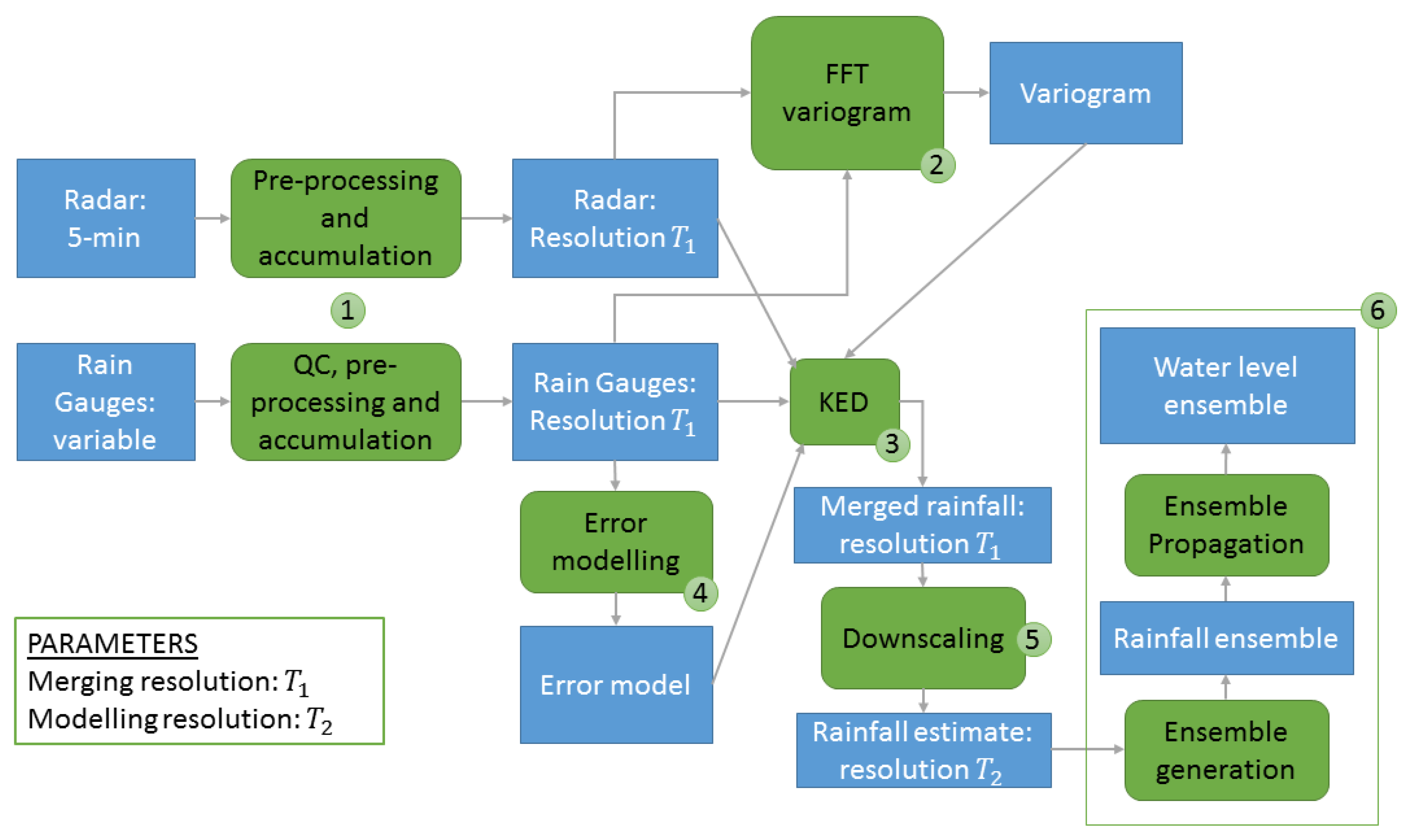
The methodology followed in this work is illustrated in Figure 4 and the passages are explained in the following sections.

3.1. Data Pre-Processing and Accumulation

3.1.1. Radar

As concerns the radar pre-processing, for each accumulation interval, all of the 5-min radar measurements available are used. The UK Met Office radar data are already corrected for errors, are available as rainfall intensity in (mm/h), and only require accumulation to $T_1$.

The KNMI data are already corrected for ground clutter and anomalous propagation as well [32], but the data are provided in (dBZ) and a conversion to (mm⁶/m³) is necessary. Then, the rainfall rate is calculated using the Z-R relationship [32]:

$$\mathrm{Z}=200 {\mathrm{R}}^{1.6}$$

(1)

As suggested by Overeem et al. [32], the values below 7 dBZ are not converted to avoid an excessive impact of noise, and are directly set to 0 mm/h. Once all the 5-min acquisitions are correctly converted from (dBZ) to rainfall rates in (mm/h), they are accumulated on the desired accumulation $T_1$.

3.1.2. Rain Gauges

The first step for rain gauge data preparation is a quality check. Rain gauge records are checked for typical malfunctioning behaviours and are compared with neighbouring rain gauges and with the radar data. In the case a rain gauge presents an anomalous behaviour (e.g., absence of records, signs of blockage, absence of zeros, etc.) for the full examined period, the rain gauge time series is removed from the dataset (as happened for the Twenterand rain gauge TWA 129 and the amateur rain gauge HWA 60); if the anomalous behaviour happens for a limited time, the affected records are substituted with “NA” (Not Available). After quality check, “NA” values affect the 3.7% of the dataset.

The EA rain gauges are already in a uniform and evenly distributed 15-min resolution, therefore accumulations can be performed directly. The rain gauges for the Dutch case study have variable accumulation times, from 3 min to one day. To correctly distribute the measured precipitation, the dataset is divided into 1 min intervals and the recorded precipitation is evenly distributed on the accumulation minutes. For example, if 10 mm are recorded over a 10 min interval, the previous 10 min will be assigned 1 mm each. Subsequently, the rain gauge records are accumulated to the desired accumulation $T_1$. This passage helps to correctly distribute measurements recorded over two or more accumulation intervals. For large accumulation times, it results in a simplification, but it is still preferred to the option of considering all the rainfall accumulation at the end of the recorded period. For example, if a daily record measures 24 mm at 08:00 (CEST). over a 24-h period, we prefer to assign 16 mm to the day before, and 8 mm to the day of the record, rather than 24 mm on the day of the record. However, it must be considered that daily records are used only for daily accumulations.

After the accumulation, a check on the convective conditions is done. When precipitation has strong convective characteristics, the reliability of the rain gauges declines, because they cannot be considered representative of the 1 km cell they belong to [8,34,35]. This effect is stronger for shorter accumulation times and can have very negative impact in the merging phase [36]. To prevent this, a convective control routine is applied, similar to the one presented by Sideris et al. [36]. For each rain gauge and for each time step, the coefficient of variation and the standard deviation of the 5 pixels by 5 pixels square around the rain gauge are calculated. The rain gauge is marked as unreliable if the coefficient of variation or the standard deviation passes an empirical threshold, dependent on the accumulation rate and on their temporal resolution. In such cases, the rain gauge is eliminated from the merging dataset for the specific time step.

3.2. Variogram Calculation

The variogram calculation presents two problems to be addressed:

• For the Dutch case study, the number of rain gauges is limited, and their resolution highly variable, therefore a reliable time-variant variogram calculation based on ground measurements is difficult to calculate.
• The variogram for KED needs to be calculated on rainfall residuals, rather than on the rainfall field itself [37].

For this reason, the following approach in four passages, based on a Fast Fourier Transform (FFT), is used for each time step:

• The variogram of the rainfall field is calculated with the FFT approach by Marcotte [38], based on the radar data [39].
• The rain gauges are interpolated applying ordinary kriging with the calculated variogram.
• The residuals are calculated subtracting the radar field from the interpolated rain gauge field.
• The variogram of the residuals is calculated with the FFT approach.

Once the empirical 2D variogram is calculated, it is fitted every 10° between 0° and 180° in azimuth (the variogram is symmetric about the 0–180° direction) with a Gaussian function:

$$\gamma \left(d\right)=\{\begin{array}{ll}0& \mathrm{for} d=0\\ c_0+c\left(1-\exp \left(-\frac{3d^2}{a^2}\right)\right)& \mathrm{for} d>0\end{array}$$

(2)

where $d$ is the distance, $c_0$ is the nugget, $c$ is the sill, and $a$ is the range. The average nugget, average sill, and average range over the tested directions are used for the merging.

3.3. Merging Using Kriging with External Drift

Universal kriging, as opposed to ordinary kriging, considers the mean of the studied field $R\left(x\right)$ non-stationary in space:

$$R\left(x\right)=m\left(x\right)+\delta \left(x\right)$$

(3)

where $m\left(x\right)$ is the mean and $\delta \left(x\right)$ is a zero-mean stationary random process [37]. Kriging with External Drift is a special case of universal kriging, in which the mean is considered a linear function of external factors. In the presented case, the mean of the rain gauge interpolation is considered a linear function of the radar rainfall estimate:

$$m\left(x\right)= {\beta }_1·r\left(x\right)+{\beta }_2$$

(4)

where $r\left(x\right)$ is the radar rainfall estimate in $x$, and ${\beta }_1$ is a linear coefficient, and ${\beta }_2$ is the intercept, to be determined.

The prediction in each point is derived from the observations with a weighted average:

$$\hat{R}\left(x_0\right)= {\displaystyle \sum }_{\alpha =1}^n{w}_{\alpha }·R\left(x_{\alpha }\right)$$

(5)

where $\hat{R}\left(x_0\right)$ is the estimated rainfall in a generic point $x_0$, $R\left(x_{\alpha }\right)$ are the measured values in the rain gauge locations $x_{\alpha }$, $n$ is the number of observations, and $w_{\alpha }$ are the kriging weights, estimated solving the kriging system:

$$\{\begin{array}{l}{\displaystyle \sum _{\alpha =1}^n}{w}_{\alpha }\left(x_0\right)=1\\ {\displaystyle \sum _{\alpha =1}^n}{w}_{\alpha }\left(x_0\right)·C\left(x_{\beta }-x_{\alpha }\right)+{\mu }_1+{\mu }_2·r\left(x_{\beta }\right)=C\left(x_{\beta }-x_0\right)\hspace{1em}\beta =1,\dots , n\\ {\displaystyle \sum _{\alpha =1}^n}{w}_{\alpha }\left(x_0\right)·r\left(x_{\alpha }\right)=r\left(x_0\right)\end{array}$$

(6)

where $C\left(d\right)$ is a covariance function, $x_{\alpha }$ and $x_{\beta }$ are generic rain gauge locations, $r\left(x\right)$ is the radar rainfall estimate in the position $x$, and ${\mu }_1$ and ${\mu }_2$ are Lagrange parameters [37]. The covariance function $C\left(d\right)$ is directly related to the variogram function $\gamma \left(d\right)$ fitted with a Gaussian model as follow:

$$C\left(d\right)=c+c_0-\gamma \left(d\right)= \{\begin{array}{ll}c+c_0& \hspace{1em}\mathrm{for} d=0\\ c\left(\exp \left(-\frac{3d^2}{a^2}\right)\right)& \hspace{1em}\mathrm{for} d>0\end{array}$$

(7)

The solution of such a system can be expressed in matrix form:

$$\mathit{W}={\mathit{C}}^{-1}·\mathit{D}=\left[\begin{array}{c}{w}_1\\ w_2\\ ⋮\\ w_n\\ {\mu }_1\\ {\mu }_2\end{array}\right]= {\left[\begin{array}{cccccc}{C}_{11}& C_{12}& \dots & C_{1n}& 1& r_1\\ C_{21}& C_{22}& \dots & C_{2n}& 1& r_2\\ ⋮& ⋮& \ddots & ⋮& ⋮& ⋮\\ C_{n1}& C_{n2}& \dots & C_{nn}& 1& r_n\\ 1& 1& \dots & 1& 0& 0\\ r_1& r_2& \dots & r_n& 0& 0\end{array}\right]}^{-1}·\left[\begin{array}{c}{C}_{10}\\ C_{20}\\ ⋮\\ C_{n0}\\ 1\\ r_0\end{array}\right]$$

(8)

where $r_i$ are the radar measurement at rain gauge locations $x_i$, while $r_0$ is the radar measurement in the prediction location $x_0$. The matrix elements $C_{ij}$ represent the covariance function calculated on the distance between $x_i$ and $x_j$.

The kriging mean and variance for each point $x_0$ are then calculated as:

$$\hat{R}\left(x_0\right)={\mathit{W}}^T·\mathit{R}$$

(9)

$${\sigma }^2\left(x_0\right)=c -{\mathit{W}}^T·\mathit{D}$$

(10)

where $\mathit{R}$ is the vector of the measurements at rain gauge locations.

3.4. Rain Gauge Error Modelling

The rain gauge errors can be included in the merging process using a Kriging for Uncertain Data (KUD) approach similar to the one by [40], assuming that the rain gauges are affected only by random errors, and that biases are already removed with calibration.

The idea is that rain gauge random errors can be modelled as a nugget effect in the variogram [37,41]. To model a different error for different rain gauges, the covariance matrix $\mathit{C}$ needs to be modified. The advantage of using a covariance function rather than a variogram function, as in most kriging formulations [37,40,42], is that the covariance function is affected by the nugget only at distance $d=0$, therefore the covariance matrix modification is simple:

$$C= \left[\begin{array}{cccccc}{C}_{11}+c_{0_1}& C_{12}& \dots & C_{1n}& 1& r_1\\ C_{21}& C_{22}+c_{0_2}& \dots & C_{2n}& 1& r_2\\ ⋮& ⋮& \ddots & ⋮& ⋮& ⋮\\ C_{n1}& C_{n2}& \dots & C_{nn}+c_{0_n}& 1& r_n\\ 1& 1& \dots & 1& 0& 0\\ r_1& r_2& \dots & r_n& 0& 0\end{array}\right]$$

(11)

where $c_{0_i}$ is the nugget effect due to the uncertainty of the $i^{th}$ rain gauge. The nugget effect for each rain gauge can be calculated separately using the rain gauge error models illustrated below, that calculate the error as function of the rainfall rate $R\left(t,x_i\right)$, and of the accumulation $T_1$.

3.4.1. Tipping Bucket Rain Gauge Error Model

The random errors for tipping bucket rain gauges are modelled according to the model by Ciach [43]. This error model is applied to the rain gauges in the UK case study, to the ones from the Municipality of Twenterand (TWE), and to the rain gauges from the Het Weer Actueel network (HWA). The standard error is calculated as:

$${\sigma }_{\mathrm{err}}\left(T_1,R_T\right)= e_0\left(T_1\right)+\frac{R_0\left(T_1\right)}{R_T}$$

(12)

where $R_T$ is the rainfall intensity at accumulation $T=T_1$ minutes, while $e_0\left(T\right)$ and $R_0\left(T\right)$ are coefficients dependant on the accumulation time. Figure 6 in Ciach’s work [43] shows the errors of the rain gauge data. Using this figure, we derived an approximated analytical formulation where $T_1$ is expressed in minutes:

$${\log }_{10}\left(e_0(T_1)\right) = -0.5923·{\log }_{10}{T}_1-1.4163$$

(13)

$${\log }_{10}\left(R_0(T_1)\right)= -0.8789·{\log }_{10}{T}_1+0.7363$$

(14)

For each tipping bucket rain gauge at each time step, for each accumulation $T_1$, the nugget can be calculated as:

$$c_{0_i}\left(t,T_1\right)= {\sigma }_{\mathrm{err}}{\left(T_1,R_T(t,x_i)\right)}^2={\left(e_0\left(T_1\right)+\frac{R_0\left(T_1\right)}{R_T\left(t,x_i\right)}\right)}^2$$

(15)

3.4.2. KNMI Automatic Rain Gauges

KNMI automatic rain gauges are not tipping bucket devices. They measure the water level using the accurate measurement of a floating device position on the water surface. This type of rain gauges is more precise than the tipping bucket type, especially at low rainfall intensity, it is subject to less measuring errors, and it is calibrated by the KNMI [31,44].

A quantitative measurement of the KNMI automatic rain gauge accuracy can be derived from the laboratory test results reported in the KNMI technical report TR-287 [44], studying and comparing the accuracy of several rain gauges, in order to select devices able to meet the World Meteorological Organisation standards.

In particular, the results reported in Section 3.2 and Figure 57 of the TR-287 report [44], show that the KNMI automatic rain gauges, after calibration, have an error around 1% at 1-min averaging, for intensities between 0 and 270 mm/h.

Considering that, in this work, we use different accumulations, the errors can be calculated considering the variance sum property:

$$Var\left({\displaystyle \sum }_{i=1}^n{X}_i\right)= {\displaystyle \sum }_{i,j=1}^{n}Cov\left(X_i,X_j\right)$$

(16)

where $X$ is a general variable, $i$ and $j$ are generic indices.

In the case of rainfall accumulation, the variable to be summed are rainfall intensities at 1-min resolution, recorded at different time steps. The covariance between two generic 1-min rainfall intensities is not known. We propose to estimate an approximation of it using the rainfall auto-correlation function. The rain gauge data from all the networks for the studied event are used to calculate the rainfall auto-correlation:

$$\widehat{AC}\left(\tau \right)=\frac{E\left\{\left(R_t-\mu \right)\left(R_{t+\tau }-\mu \right)\right\}}{{\sigma }^2}$$

(17)

where, $\widehat{AC}\left(\tau \right)$ is the auto-correlation, $\tau$ is a generic time interval, $R_t$ is the rainfall intensity at time $t$, whereas $\mu$ and ${\sigma }^2$ are, respectively, the mean and the variance of the rainfall over the time series; the process is considered stationary for simplicity.

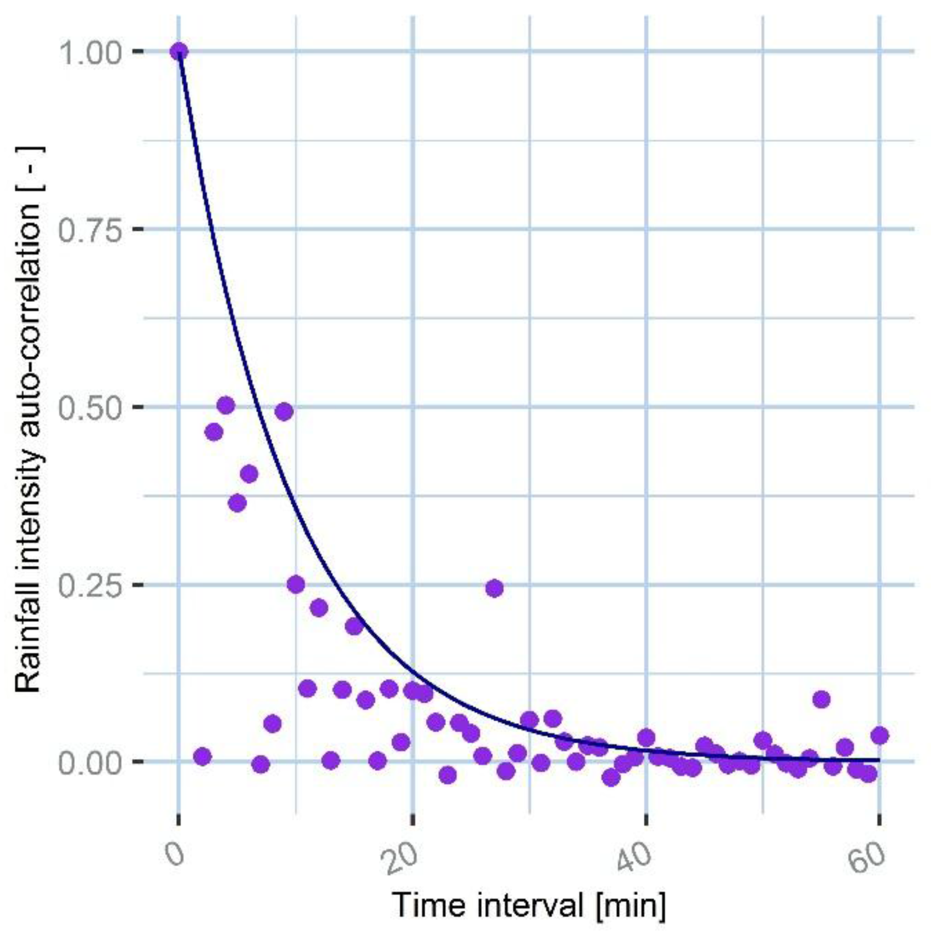
The auto-correlation is then fitted using an auto-correlation function with an exponential form:

$$AC\left(\tau \right)=\exp \left(b·\tau \right)$$

(18)

The exponential fitting of the rainfall auto-correlation function is shown in Figure 5.

Knowing the auto-correlation function, Equation (16) can be expanded:

$$Var\left(R_T\right)= {\displaystyle \sum }_{i=1}^T{\displaystyle \sum }_{j=1}^{T}CO{V}_{i,j}=Var\left(R_1\right)· {\displaystyle \sum }_{i=1}^T{\displaystyle \sum }_{j=1}^{T}A{C}_{i,j}$$

(19)

where $R_T$ is the rainfall intensity at accumulation $T=T_1$ minutes, $R_1$ is the rainfall intensity at accumulation $T=1$ min, $CO{V}_{i,j}$ are the elements of the covariance matrix $COV$ between all the 1-min measurements in a $T_1$-minutes interval, and $A{C}_{i,j}$ are the elements of the auto-correlation matrix $\mathit{A}\mathit{C}$, defined as follows:

$$\mathit{A}\mathit{C}= \left[\begin{array}{ccccc}AC\left(0\right)& AC\left(1\right)& AC\left(2\right)& \cdots & AC\left(T_1\right)\\ AC\left(1\right)& AC\left(0\right)& AC\left(1\right)& \cdots & AC\left(T_1-1\right)\\ AC\left(2\right)& AC\left(1\right)& AC\left(0\right)& \cdots & AC\left(T_1-2\right)\\ ⋮& ⋮& ⋮& \ddots & ⋮\\ AC\left(T_1\right)& AC\left(T_1-1\right)& AC\left(T_1-2\right)& \cdots & AC\left(0\right)\end{array}\right]$$

(20)

where $\mathit{A}\mathit{C}\left(\tau \right)$ is the function derived from Equation (18) with the interval in minutes.

As concerns the variance element $Var\left(R_1\right)$, it is defined following the KNMI report, as the square of the 1% of the rainfall intensity at 1-min accumulation. Since the rainfall intensity at 1-min accumulation is not known, because the KNMI data are available at hourly accumulation, it can be approximated as function of the accumulation time $T_1$:

$$Var\left(R_1\right)={\left(1\% R_1\right)}^2={\left(1\%\frac{R_T}{T_1}\right)}^2$$

(21)

Combining Equations (19)–(21), the relative error for each KNMI automatic rain gauge measurement in position x, at time t, and accumulation $T_1$ can be expressed as follows:

$${\sigma }_{\mathrm{err}}\left(T_1, R_T(t, x_i)\right)=a\left(T_1\right)·R_T\left(t, x_i\right)$$

(22)

where

$$a\left(T_1\right)=\left(\frac{1\%}{T_1}\right)\sqrt{{\displaystyle \sum }_{i,j=1}^{T}A{C}_{i,j}}$$

(23)

The corresponding nugget effect, for the application of Equation (11), is:

$$c_{0_i}\left(t,T_1\right)={\sigma }_{\mathrm{err}}{\left(T_1, R_T(t, x_i)\right)}^2$$

(24)

3.4.3. KNMI Manual Rain Gauges

The KNMI manual rain gauges are based on a water level system; each day volunteers and amateurs read the water level at 08:00 (CEST) and communicate the reading to the KNMI. The KNMI Technical Report TR-347 provides an estimate of the manual rain gauge uncertainty [31]. Differently from the previous error models that are considered bias-free, the report suggests that the KNMI manual rain gauges are affected by bias and we derived a correction.

In particular, we combined the information from Figures 14 and 16 of the TR-347 report [31] to derive the following bias correction and error estimate as function of the rainfall rate:

$$R^{\ast }\left(t, x_i\right)=R\left(t, x_i\right)·\left(1-0.125·R{\left(t, x_i\right)}^{-0.372}\right)$$

(25)

$${\sigma }_{\mathrm{err}}\left(R\left(t,x_i\right)\right)=R\left(t, x_i\right)·\left(0.0489·R{\left(t, x_i\right)}^{-0.447}\right)$$

(26)

where $R^{\ast }\left(t, x_i\right)$ is the bias corrected rainfall rate at time t and position $x_i$, $R\left(t,x_i\right)$ is the original rainfall rate before correction, and ${\sigma }_{\mathrm{err}}\left(R(t,x_i)\right)$ is the standard deviation. The corresponding nugget is derived from Equation (24). The standard deviation calculation in Equation (26) is derived from the report and is a function of the original rainfall rate, before bias correction.

3.5. Downscaling

Once the KED produces a probabilistic estimation of the rainfall intensity at temporal accumulation $T_1$, we need to downscale it to the desired temporal resolution $T_2$. The probabilistic estimate is made of a prediction and a variance estimate, and both need to be downscaled.

3.5.1. Downscaling the KED Prediction

To downscale the prediction, the original radar acquisitions are used to determine how to distribute the accumulated KED rainfall $R_{\mathrm{KED}.T_1}\left(t\right)$ among the time steps at resolution $T_2$:

$$R_{\mathrm{KED}.T_2}\left(x,t\right)=R_{\mathrm{rad}.T_2}\left(x,t\right)·\frac{R_{\mathrm{KED}.T_1}\left(x,t\right)}{R_{\mathrm{rad}.T_1}\left(x,t\right)}$$

(27)

where $R_{\mathrm{KED}.T_1}\left(x,t\right)$ is the KED prediction at accumulation $T_1$, for position $x$ and time step $t$; $R_{\mathrm{rad}.T_1}\left(x,t\right)$ is the accumulation at $T_1$ of the uncorrected radar acquisitions; $R_{\mathrm{rad}.T_2}\left(x,t\right)$ is calculated accumulating the uncorrected radar at $T_2$; and $R_{\mathrm{KED}.T_2}\left(x,t\right)$ is the downscaled KED estimation at $T_2$. Since the radar has a resolution of 5 min, the downscaling resolution $T_2$ has to be a multiple of 5 min.

To avoid divisions by zero or near-zero values, 0.00001 mm are added to the uncorrected radar estimates before accumulations, therefore both $R_{\mathrm{rad}.T_2}\left(x,t\right)$ and $R_{\mathrm{rad}.T_1}\left(x,t\right)$, derived as accumulations of uncorrected radar estimates at $T_2$ and $T_1$ respectively, will be increased of 0.00001 mm for each contained radar estimate.

3.5.2. Downscaling the KED Variance

As regards the variance, the downscaling is based on two principles:

• The variance of a sum is the sum of the covariance between all summed elements (Equation (16)).
• The standard deviation is proportional to the rainfall rate. This comes from the fact that both radar and rain gauges are affected mainly by multiplicative errors [43,45,46,47].

From the first principle and Equation (16) we can derive:

$$Var\left(R_{\mathrm{KED}.T_1}(x,t)\right)= \overline{Var\left(R_{\mathrm{KED}.T_2}(x,t)\right)}· {\displaystyle \sum }_{i,j=1}^{T_1/T_2}AC{2}_{i,j}$$

(28)

where $\overline{\left(Var\left(R_{\mathrm{KED}.T_2}\left(x,t\right)\right)\right)}$ is the mean variance value for all the time steps at $T_2$ resolution contained in each time step at $T_1$ accumulation; $AC{2}_{i,j}$ are the elements of an auto-correlation matrix similar to the one defined in Equation (20), but defined at time steps equal to $T_2$, that is:

$$\mathit{A}\mathit{C}\mathbf{2}= \left[\begin{array}{ccccc}AC\left(0\right)& AC\left(T_2\right)& AC\left(2T_2\right)& \cdots & AC\left(T_1\right)\\ AC\left(T_2\right)& AC\left(0\right)& AC\left(T_2\right)& \cdots & AC\left(T_1-T_2\right)\\ AC\left(2T_2\right)& AC\left(T_2\right)& AC\left(0\right)& \cdots & AC\left(T_1-2T_2\right)\\ ⋮& ⋮& ⋮& \ddots & ⋮\\ AC\left(T_1\right)& AC\left(T_1-T_2\right)& AC\left(T_1-2T_2\right)& \cdots & AC\left(0\right)\end{array}\right]$$

(29)

To comply with the second principle instead, the following equation is derived:

$$SD\left(R_{\mathrm{KED}.T_2}(x,t)\right)=\frac{R_{\mathrm{rad}.T_2}\left(x,t\right)}{R_{\mathrm{rad}.T_1}\left(x,t\right)}·\frac{T_1}{T_2}·\overline{SD\left(R_{\mathrm{KED}.T_2}(x,t)\right)}$$

(30)

where $SD\left(R_{\mathrm{KED}.T_2}(x,t)\right)$ is the actual standard deviation at resolution $T_2$ while $\overline{\left(SD\left(R_{\mathrm{KED}.T_2}(x,t)\right)\right)}$ is the average standard deviation of all the prediction at resolution $T_2$ contained in each time step at resolution $T_1$. $R_{\mathrm{rad}.T_2}\left(x,t\right)$ and $R_{\mathrm{rad}.T_1}\left(x,t\right)$ are, respectively, the uncorrected radar estimates accumulated to $T_2$ and $T_1$.

Combining Equations (28) and (30):

$$Var\left(R_{\mathrm{KED}.T_2}(x,t)\right)={\left(\frac{R_{\mathrm{rad}.T_2}\left(x,t\right)}{R_{\mathrm{rad}.T_1}\left(x,t\right)}·\frac{T_1}{T_2}\right)}^2·\frac{Var\left(R_{\mathrm{KED}.T_1}(x,t)\right)}{{{\displaystyle \sum }}_{i,j=1}^{T_1/T_2}AC{2}_{i,j}}$$

(31)

As in the prediction downscaling phase, to avoid divisions by zero or near-zero values, 0.00001 mm are added to the uncorrected radar estimates before accumulation, therefore both $R_{\mathrm{rad}.T_2}\left(x,t\right)$ and $R_{\mathrm{rad}.T_1}\left(x,t\right)$, derived as accumulations of uncorrected radar estimates at $T_2$ and $T_1$, respectively, will be increased by 0.00001 mm for each contained radar estimate.

3.6. Ensemble Generation and Propagation

Once a probabilistic estimate is derived, the uncertainty can be propagated with an ensemble, i.e., a collection of a large number of possible alternative realisations of rainfall time series.

Each ensemble member is modelled as:

$$R_{{\mathrm{ens}}_i}\left(x,t\right)= R_{\mathrm{KED}.T_2}\left(x,t\right)+SD\left(R_{\mathrm{KED}.T_2}(x,t)\right)·{ϵ}_i(x,t)$$

(32)

where $R_{{\mathrm{ens}}_i}\left(x,t\right)$ is the $i^{th}$ ensemble member; $R_{\mathrm{KED}.T_2}\left(x,t\right)$ and $SD\left(R_{\mathrm{KED}.T_2}\left(x,t\right)\right)$ are, respectively, the downscaled KED mean and the downscaled KED standard deviation; and ${ϵ}_i\left(x,t\right)$ is a standardized, zero-mean, spatially auto-correlated residual field.

To generate ${ϵ}_i\left(x,t\right)$, an unconditional simulation is used, with mean equal to zero, and standard deviation equal to one, using the residuals’ variogram at the corresponding time step. Subsequently, in order to reconstruct the auto-correlation of the residuals, a $AR\left(2\right)$ model is used. The auto-correlation and the parameters of the $AR\left(2\right)$ model are derived from the residuals time series, calculated as in Section 3.2.

4. Results

4.1. Case Study 1: Evaluation of the Optimal Combination in Terms of Rainfall Product Quality

The case study based in the UK has been used to validate the methodologies in terms of ability to reproduce the observed rainfall. This case study does not bring any information about the optimization of the rainfall for urban modelling applications, but proves that the used techniques are able to reproduce reasonable rainfall products. While the case study in the UK was suitable to validate the methodology, thanks to the large number of rain gauges and the uniform data quality, an urban model was not available; at the same time, the case study in the Netherlands was not suitable for validation, due to the limited number of rain gauges and the variable data quality, but allowed an urban modelling application. Therefore, two case studies are here presented. The same methodology used to generate the rainfall products has been used; in the first case study, the results have been cross-validated, while, in the second, they are applied to an urban drainage model and the uncertainty is estimated and propagated. The cross-validation is evaluated with the same skill scores used for the Dutch case study, although it must be kept in mind that the evaluated quantity is different (in the first case study it is based on rainfall intensity, while, in the second case study, it is based on water levels). Three indicators are calculated: Bias, Mean Root Transformed Error (MRTE), and Nash–Sutcliff Efficiency (NSE).

$$\mathrm{BIAS}=abs\left(\frac{1}{t_{\mathrm{steps}}}{\displaystyle \sum }_{j=1}^{t_{\mathrm{steps}}}{R}_{\mathrm{KED}}-R_{\mathrm{obs}}\right)$$

(33)

$$\mathrm{MRTE}=\frac{1}{t_{\mathrm{steps}}}{\displaystyle \sum }_{j=1}^{t_{\mathrm{steps}}}{\left(\sqrt{R_{\mathrm{KED}}}- \sqrt{R_{\mathrm{obs}}}\right)}^2$$

(34)

$$\mathrm{NSE}=1-\frac{{{\displaystyle \sum }}_{j=1}^{t_{\mathrm{steps}}}{\left(R_{\mathrm{obs}}- R_{\mathrm{KED}}\right)}^2}{{{\displaystyle \sum }}_{j=1}^{t_{\mathrm{steps}}}{\left(R_{\mathrm{obs}}-\overline{R_{\mathrm{obs}}}\right)}^2}$$

(35)

where $t_{\mathrm{steps}}$ is the number of considered time steps in the event, $R_{\mathrm{KED}}$ is the rainfall intensity estimated with KED, $R_{\mathrm{obs}}$ is the rainfall intensity observed by the validation rain gauges, and $\overline{R_{\mathrm{obs}}}$ is the average observed rainfall intensity. The bias and the MRTE are optimal when they tend to 0, while the NSE is optimal when it tends to 1. The three indicators are calculated for each of the 12 tested rainfall products. The results of the cross-validation are reported in

Table 6. The three indicators (bias, MRTE, and NSE) are reported for the 12 products of the UK case study, indicated with accumulation resolution (A) and downscaling resolution (D) in minutes. A conditional colour formatting is applied to easily compare the values, where green is a positive performance, and red a negative one.

BIAS
A\D	15	30	60
60	0.065	0.069	0.078
180	0.054	0.056	0.064
720	0.048	0.045	0.051
1440	0.045	0.043	0.045
MRTE
A\D	15	30	60
60	0.193	0.166	0.147
180	0.187	0.161	0.142
720	0.165	0.139	0.123
1440	0.147	0.127	0.113
NSE
A\D	15	30	60
60	0.46	0.52	0.58
180	0.46	0.51	0.55
720	0.51	0.55	0.59
1440	0.52	0.56	0.59

.

Additionally, we want to investigate how well the uncertainty is estimated. To do so, we use rank histograms with a variation. Rank histograms are a tool used to evaluate a probabilistic prediction with a deterministic observation and are built looking in which prediction quantile the observation falls, for each time step and each rain gauge. The rank histogram shows how often the observation falls in each of the prediction quantiles. However, in this case, we want to consider the observation uncertainty too, as modelled in Section 3.4.1. For this reason, we select the prediction quantile where the product of the prediction probability and the observation probability is maximum.

The rank histograms for the tested combinations are reported in Figure 6.

4.2. Case Study 2: Identification of the Optimal Accumulation and Downscaling Resolution

In the second case study in the Netherlands, the first passage is to identify which of the 14 tested rainfall combinations is optimal in terms of reproducing the water level observations, when used as an input in the presented InfoWorks model. The 14 different products are therefore directly used in the InfoWorks model, and the results are compared to water level observations. Figure 7 shows how the model outputs for the 14 tested products compare to the observations, for the three tested measuring points of Figure 2 and Figure 3.

To have a quantitative measurement of the products’ performance, three indicators are calculated: Bias, Mean Root Transformed Error (MRTE), and Nash–Sutcliff Efficiency (NSE).

$$\mathrm{BIAS}=\mathrm{abs}\left(\frac{1}{t_{\mathrm{steps}}}{\displaystyle \sum }_{j=1}^{t_{\mathrm{steps}}}{h}_{\mathrm{mod}}-h_{\mathrm{obs}}\right)$$

(36)

$$\mathrm{MRTE}=\frac{1}{t_{\mathrm{steps}}}{\displaystyle \sum }_{j=1}^{t_{\mathrm{steps}}}{\left(\sqrt{h_{\mathrm{mod}}}- \sqrt{h_{\mathrm{obs}}}\right)}^2$$

(37)

$$\mathrm{NSE}=1-\frac{{{\displaystyle \sum }}_{j=1}^{t_{\mathrm{steps}}}{\left(h_{\mathrm{obs}}- h_{\mathrm{mod}}\right)}^2}{{{\displaystyle \sum }}_{j=1}^{t_{\mathrm{steps}}}{\left(h_{\mathrm{obs}}-\overline{h_{\mathrm{obs}}}\right)}^2}$$

(38)

where $t_{\mathrm{steps}}$ is the number of considered time steps in the event, $h_{\mathrm{mod}}$ is the water level estimated by the model, $h_{\mathrm{obs}}$ is the observed water level, and $\overline{h_{\mathrm{obs}}}$ is the average observed water level. The three indicators are calculated for each of the 14 tested rainfall products, and for each of the three measurement locations. The results are reported in

Table 7. The three indicators (bias, Mean Root Transformed Error—MRTE, and Nash-Sutcliffe Efficiency—NSE) are reported for the 14 products indicated with accumulation resolution (A) and downscaling resolution (D) in minutes, for the three measurement locations. Radar products are indicated with RD. A conditional colour formatting is applied to easily compare the values, where green is a positive performance, and red a negative one.

A	D	VW162			VW984C1			VW263
		BIAS	MRTE	NSE	BIAS	MRTE	NSE	BIAS	MRTE	NSE
1440	5	0.146	0.0092	0.58	0.052	0.0059	0.57	0.396	0.0177	0.02
1440	15	0.147	0.0093	0.58	0.052	0.0060	0.57	0.400	0.0182	-0.01
1440	30	0.146	0.0093	0.58	0.051	0.0060	0.57	0.399	0.0180	0.01
720	5	0.159	0.0092	0.58	0.053	0.0059	0.57	0.310	0.0103	0.44
720	15	0.159	0.0092	0.58	0.053	0.0059	0.57	0.313	0.0104	0.44
720	30	0.158	0.0092	0.58	0.052	0.0060	0.57	0.313	0.0103	0.44
180	5	0.178	0.0061	0.73	0.070	0.0033	0.77	0.303	0.0088	0.53
180	15	0.178	0.0061	0.73	0.070	0.0033	0.77	0.304	0.0088	0.53
180	30	0.178	0.0059	0.74	0.071	0.0031	0.78	0.305	0.0089	0.53
60	5	0.183	0.0061	0.73	0.072	0.0033	0.77	0.272	0.0066	0.65
60	15	0.183	0.0061	0.73	0.071	0.0033	0.77	0.271	0.0066	0.65
60	30	0.182	0.0059	0.74	0.071	0.0031	0.79	0.274	0.0066	0.65
RD	15	0.184	0.0093	0.58	0.074	0.0058	0.59	0.298	0.0101	0.46
RD	5	0.184	0.0094	0.58	0.075	0.0058	0.59	0.297	0.0102	0.46

.

4.3. Case Study 2: Ensemble Generation and Propagation

Once the optimal accumulation and downscaling resolution are selected, the corresponding downscaled KED product is considered in its probabilistic form, in order to study the uncertainty in the rainfall estimation and its propagation in the sewer model.

An ensemble of 100 rainfall estimates is generated using the methodology illustrated in Section 3.6 and each member is used as an input for the InfoWorks model, obtaining an ensemble of 100 water level estimates. The results are represented in Figure 8.

5. Discussion

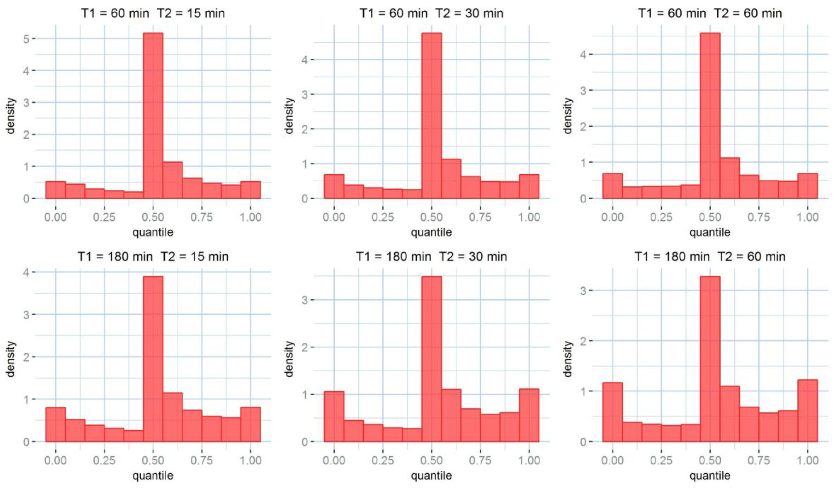
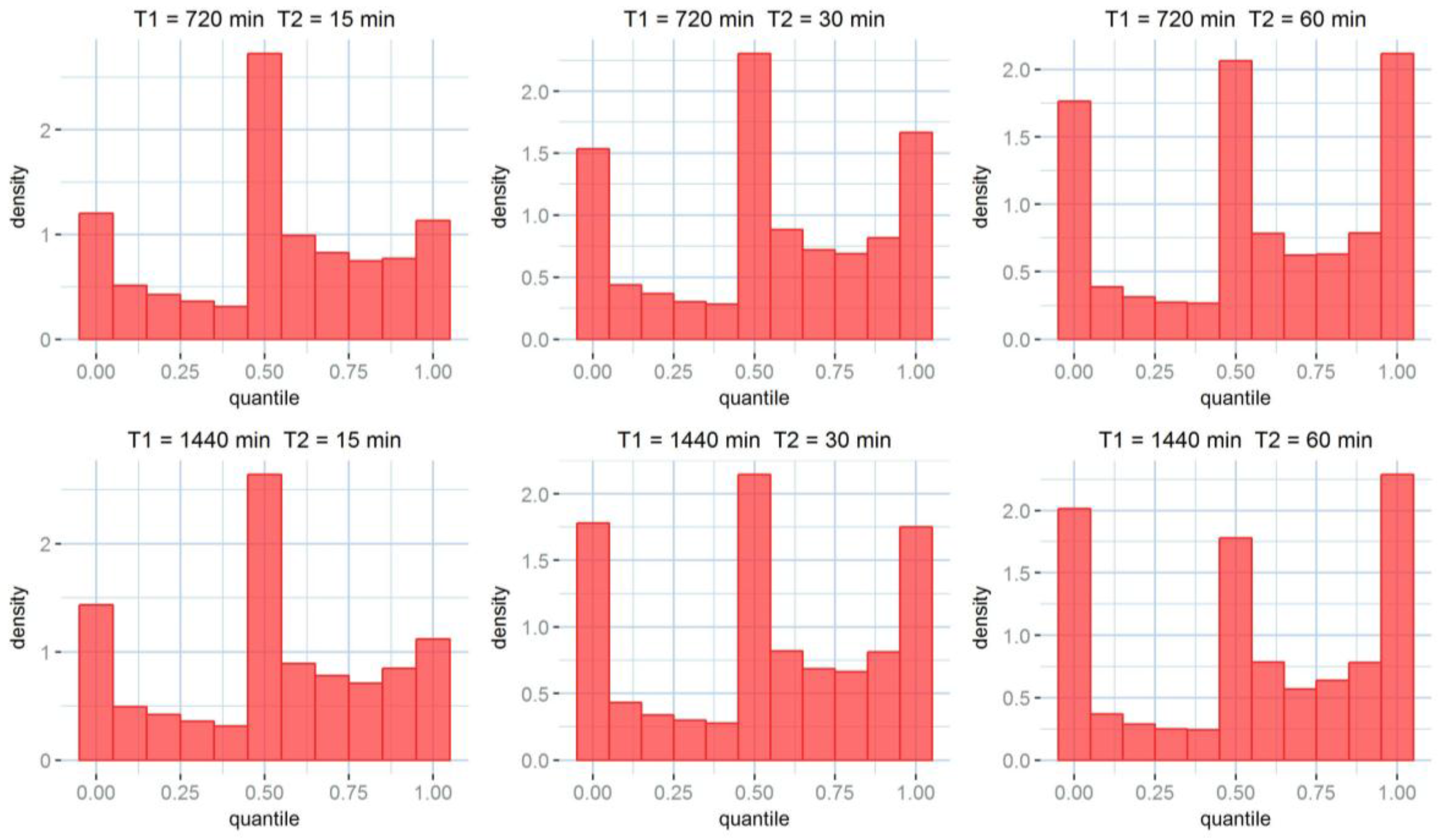
As regards the results of the methodology validation for the UK case study, as reported in Section 4.1 and Table 6, it is no surprise that larger accumulations tend to perform better. As expected, the uncertainty on the rainfall products is reduced by accumulation. Larger accumulation resolutions, associated with larger downscaling resolutions perform best for all the tested skill scores. It must be noted that the cross-validation is done between Kriging products and rain gauges; therefore, an error is always present, even for the case at 60 min accumulation and no (60 min) downscaling. The uncertainty estimation, as illustrated by the rank histograms in Figure 6, performs better at larger accumulations as well. In facts, if a perfect stochastic model were used, modelling a perfectly Gaussian process, and infinite observation points were available, rank histograms would be perfectly flat. This is not the case for any of the model histograms. Indeed, kriging produces a Gaussian probabilistic estimation, although rainfall errors are not Gaussian. Rainfall error probability distribution has a higher kurtosis, which results in a higher density of observations in the central and the extreme quantiles. While this is clearly visible for the coarser accumulations, the histograms relative to the finer accumulation scales show only a central higher peak. This usually corresponds to an overestimation of the uncertainty.

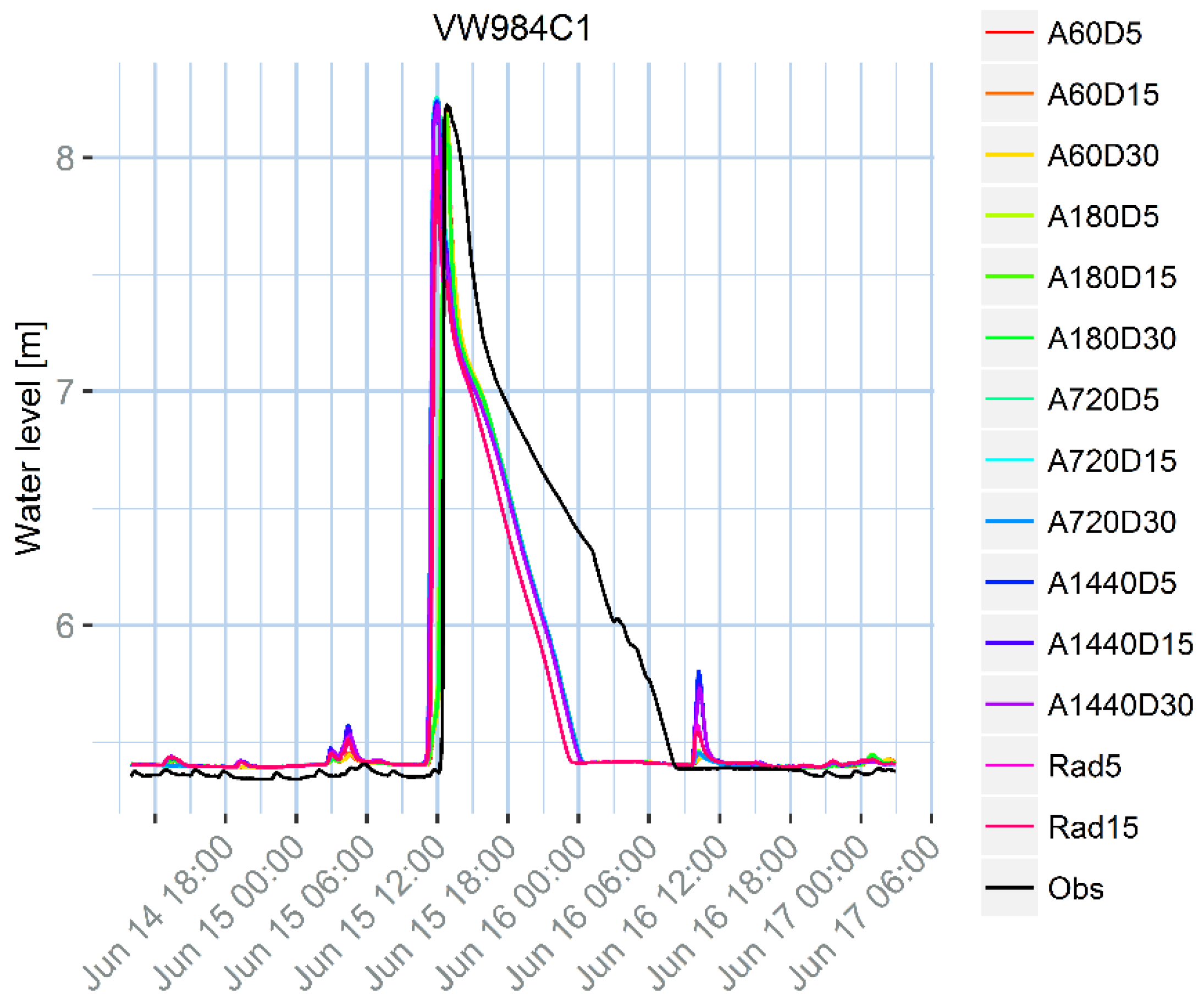
As concerns the example application in Twenterand, the first observable result from Section 4.2, Figure 7 is that the model is not appropriately calibrated for the studied event. The model is calibrated following the C2100 guideline [33], which is the standard nation-wide calibration procedure. Although the calibration aims at obtaining a set of parameters that performs well in a number of design storms with different return periods, it cannot perform at the highest standard in all the situations, since some parameters are actually not stationary. Additionally, the model is designed to properly model the flow in pressurized conducts, but does not properly represent surface water storage that can happen during a flood. This generates a mismatch between the model results and the observations that might not be due to the rainfall uncertainty, and is similar for all the tested rainfall products. For example, at location VW263 there is an evident bias, while in locations VW162 and VW984C1 the peak water level decreases too fast, compared to the observations. Additionally, some other sources of uncertainty can contribute to the mismatch, for example the inflow due to the urban sewage component, the uncertainty on the water level observations, or the model structure. In location VW263, the peak shows a different pattern compared to the observation. This effect might be linked to the presence of a pump close by, which may be modelled in an over-simplified way.

The evident mismatch between the model and the observations does not prevent the methodology presented in this work to be effective, and presents a real case scenario: as mentioned before, operational models are often calibrated against a number of design rainfall events, but cannot be optimal in all the cases. We want to propose a methodology that is effective regardless of the other additional sources of uncertainty that may affect the model. However, it could be argued that the results are affected by the non-optimal working conditions of the model. This is indeed true, and it must be kept in mind that the optimization in such conditions is specific for the given model, in the given conditions and cannot be generalized. The presented case study should be considered only as an application example of the proposed methodology and no generalization on the obtained results should be drawn.

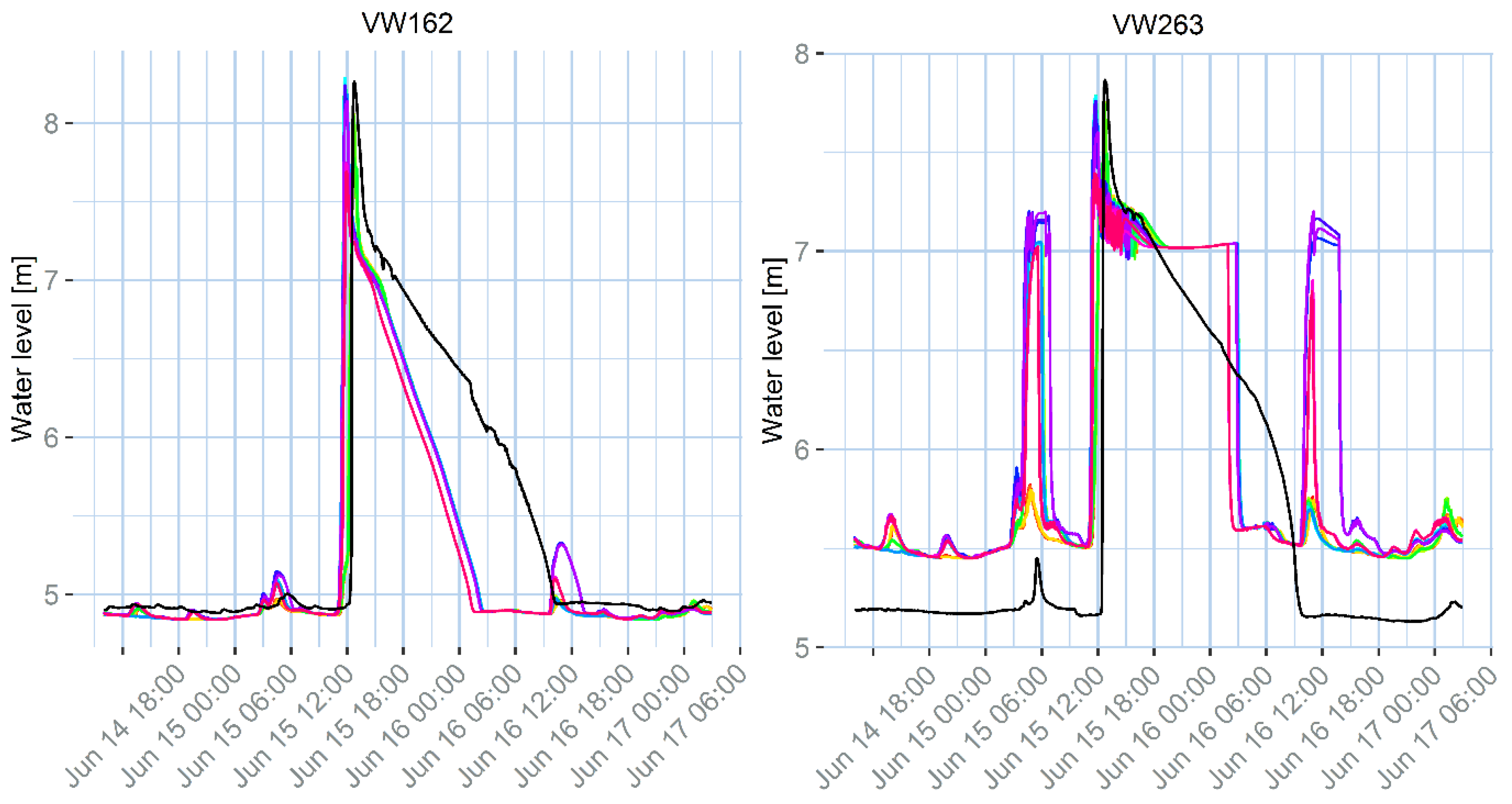
Although the differences between the rainfall products are small compared to the mismatch between the model outputs and the water level observations, there are some noticeable differences, especially for minor peaks, that can still help us in selecting the best rainfall input. The first and the last minor peaks generated by the model for the VW263 measurement point are too high for daily accumulations (1440 min), but reasonably low for accumulations between 60 min and 12 h (720 min). The same effect can be observed for the small peaks following the major ones for locations VW162 and VW984C1.

The results in Table 7 show that different products perform differently for the three measurement points. Nevertheless, it is possible to evaluate which ones perform sufficiently well in all the cases. In terms of accumulation interval, the best results are obtained for an accumulation of three hours (180 min). Sixty-minute products perform well too, but have a more variable behaviour in the different analysed cases. In terms of downscaling time, the differences are smaller, but the products downscaled at 30 min tend to perform slightly better, especially for the accumulations at 3 h. This is probably due to the reduction in rainfall errors thanks to a coarser accumulation, rather than an advantage at model level. Although, in this application, we select the product downscaled at 30 min, the other downscaling resolutions would work similarly well. Indeed, urban drainage models often work better at finer resolutions [2,48,49]. However, both the rain gauges and the radar used are subject to non-negligible errors and the reduction of uncertainty due to accumulation seems dominant in respect to the reduction of uncertainty due to the model capacity to represent finer temporal scales.

The validation results are not in contrast with the results of the Dutch case study, used to optimise the resolution for modelling application. Indeed, the downscaling brings an advantage in the model application, where finer scale phenomena need to be represented correctly. The fact that the optimal downscaling resolution has been found at 30 min is due to the balance between the rainfall uncertainty reduction at larger downscaling resolutions, and the model uncertainty reduction at smaller downscaling resolutions. In fact, it can be observed that the differences between the results at different downscaling resolutions at model level in the second case study are much smaller than the differences at rainfall level in the first case study, where larger downscaling resolutions clearly produce better results.

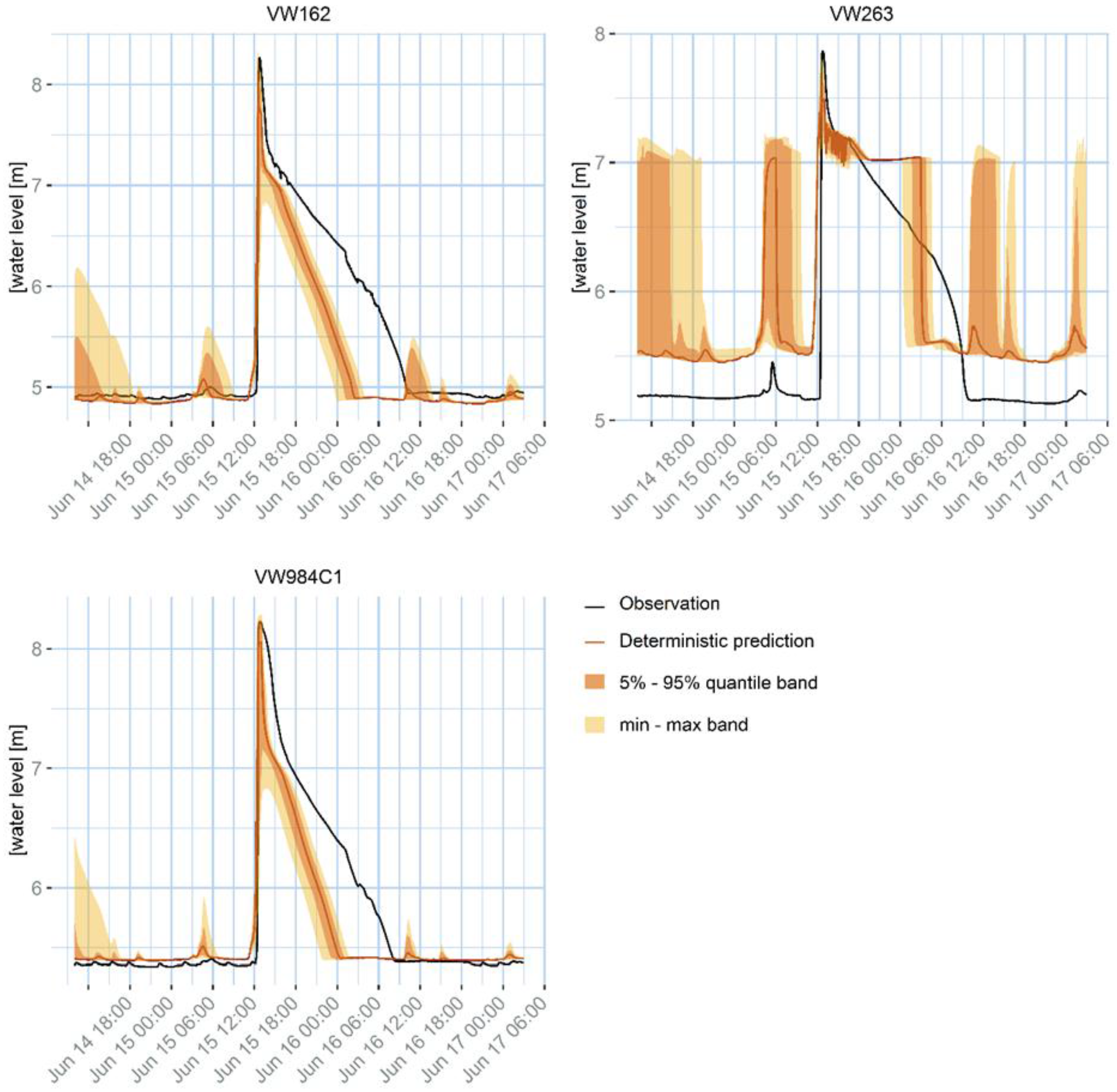
The results of the uncertainty propagation, as reported in Section 4.3, Figure 8, show that the rainfall uncertainty is not sufficient to explain the mismatch with the observations: as already mentioned in the previous section, the mismatch can be due to the model calibration, to other inputs’ uncertainty, to the water level observation uncertainty, and to the model simplification.

The fact that the uncertainty bands correspond to the variability of the 14 products observed in Figure 7 confirms that the uncertainty model is robust. In fact, the uncertainty model is independent on the other 13 products tested in the previous phase, but it is still able to capture the uncertainty due, in this case, to the temporal resolution uncertainty. Additionally, it covers also other sources of rainfall uncertainty, such as rain gauge errors or interpolation approximations. The fact that the uncertainty band does not always cover the water level observations, confirms that the InfoWorks model is affected by other sources of uncertainty such as calibration, model structure, or other data errors.

Additionally, the ensemble shows that the uncertainty tends to be larger in correspondence of peaks, but for some peaks the uncertainty band is much larger than for others. This is because kriging variance is proportional to the rainfall intensity and to the distance between the measurement points and the prediction points: two rainfall peaks with the same intensity can have a different associated uncertainty if they are closer or farther away from the rain gauge locations. The effect is even stronger if some measurements are missing, or removed because of convective conditions. Both the effects are realistic: rainfall uncertainty is known to be proportional to the rainfall intensity and is reasonable that the fewer measurements are available, the less certain the rainfall estimation is.

It must be noted that the InfoWorks model of Vroomshoop covers an area smaller than the one studied for the rainfall products, using therefore only a portion of the KED products. The use of a larger area for the rainfall estimation assures that the rainfall estimation is robust, while the sensitivity of the uncertainty model to the rain gauge quality assures that the uncertainty is correctly dependant on the quality of the rain gauges closer to the Vroomshoop area.

The proposed methodology is successful in improving the KED merging results for urban application, considering the associated uncertainty and its propagation to model outputs. However, some improvements could still be introduced. The tested accumulation and downscaling resolutions are just a limited number, used as an example to illustrate the methodology, rather than to actually identify the optimal resolutions with high accuracy; using a larger number of combinations could help identify the optimal resolutions more accurately. Furthermore, an existing operational model calibrated according to national guidelines was used, with some associated calibration uncertainty. The case study is informative in terms of robustness of the proposed method and in terms of evaluating the relative importance of the rainfall uncertainty in respect to the overall model uncertainty, but more precise results could have been obtained with a model calibrated specifically for the actual study event.

It must be considered that this work aims at illustrating an effective methodology for producing rainfall products optimized for a specific model, and the quantitative results are specific for the dataset and the model used. Additionally, it must be noted that this work does not aim at proposing a different merging technique; it aims at dealing with temporal scales with an existing merging technique, in this case KED. It could potentially be applied to other merging techniques, where sensitivity to rainfall data quality is noticed, and an accumulation of the rainfall data would be advisable, but, for model applications, a sufficiently fine resolution is required. It is therefore subject to the benefits and limitations of the used merging techniques.

Additionally, the ensemble generation is accomplished using an AR(2) model for the residuals auto-correlation; the AR(2) generates auto-correlated residuals, but cannot achieve the level of auto-correlation observed in the time series. A different approach could be adopted to improve the ensembles in this direction. Finally, the use of a 2D variogram approach has the potential to use an anisotropic and directional variogram for the KED merging, which was not investigated in this work.

6. Conclusions

Rainfall is a phenomenon highly variable in space and time. For this reason, a lot of effort is often put in the identification of the optimal spatio-temporal resolution for its representation, especially when it is used as input in small-scale urban models [1,2,49,50]. Although a fine resolution allows representing small-scale phenomena and provides more details, available data fix a lower limit to the achievable resolution, and accumulation is recommended to reduce the impact of random errors. Merging radar and rain gauge rainfall information is recognised to improve the rainfall estimates and Kriging with External Drift is one of the most used merging methods thanks to its good performance and efficiency [12,14,17,18]. Nevertheless, KED is sensitive to low quality data using a fine temporal scale, and accumulation is recommended [19].

This paper proposes an approach for using rainfall data accumulated to a coarser temporal resolution for KED merging, and then downscaling the results to a finer temporal scale, so it can be used in an urban hydrological model. The methodology allows to consider the uncertainty associated to the estimates as well and to propagate it in the studied model.

A first case study, based on six months of data in the north of England, is used to validate the methodology. Twelve KED products obtained using different accumulation and downscaling resolutions are cross-validated against rain gauges. The results confirm that, in terms of rainfall product quality, larger accumulations reduce the uncertainty.

Another case study in the municipality of Twenterand, in the Netherlands, is presented as an urban application example. In a first phase, 14 different rainfall products are tested, using different accumulation resolutions to perform the KED merging and different downscaling resolutions, in order to identify the optimal temporal accumulation and downscaling resolutions for the case study. Water level observations are compared to the InfoWorks results using the 14 different rainfall products as input, and the product accumulated at 3-h resolution for the KED application and then downscaled at 30-min resolution is identified as optimal in the specific application example.

For this product, the uncertainty is then considered in a second evaluation stage, and propagated in the InfoWorks model. The kriging prediction (mean) and the kriging variance are used to produce a rainfall ensemble composed of 100 alternative rainfall time series. Each ensemble member is used in the model, obtaining an ensemble of 100 alternative water level estimates.

The used InfoWorks model presents some additional sources of uncertainty, due mainly to the impossibility to model surface storage, calibration, other inputs uncertainty, model structure, or observation errors. The proposed methodology correctly estimates the uncertainty in the water level due to the rainfall uncertainty, and does not cover the whole observable mismatch between the model output and the observations. This also allows evaluating the relative importance of the rainfall uncertainty in the overall model output uncertainty.

Although some details can still be improved, the illustrated methodology is successful in generating robust and accurate rainfall estimates and associated uncertainty. The methodology can be applied to different case studies and different models and a more accurate identification of the optimal resolutions for accumulation and for downscaling is easily achievable.

References

1. Schilling, W. Rainfall data for urban hydrology: What do we need? Atmos. Res. 1991, 27, 5–21. [Google Scholar] [CrossRef]
2. Berne, A.; Delrieu, G.; Creutin, J.; Obled, C. Temporal and spatial resolution of rainfall measurements required for urban hydrology. J. Hydrol. 2004, 299, 166–179. [Google Scholar] [CrossRef]
3. Gabellani, S.; Boni, G.; Ferraris, L.; von Hardenberg, J.; Provenzale, A. Propagation of uncertainty from rainfall to runoff: A case study with a stochastic rainfall generator. Adv. Water Resour. 2007, 30, 2061–2071. [Google Scholar] [CrossRef]
4. Fletcher, T.D.; Andrieu, H.; Hamel, P. Understanding, management and modelling of urban hydrology and its consequences for receiving waters: A state of the art. Adv. Water Resour. 2013, 51, 261–279. [Google Scholar] [CrossRef]
5. Berne, A.; Krajewski, W.F. Radar for hydrology: Unfulfilled promise or unrecognized potential? Adv. Water Resour. 2013, 51, 357–366. [Google Scholar] [CrossRef]
6. Islam, T.; Rico-Ramirez, M.A. An overview of the remote sensing of precipitation with polarimetric radar. Prog. Phys. Geogr. 2013, 38, 1–24. [Google Scholar] [CrossRef]
7. Villarini, G.; Krajewski, W.F. Review of the different sources of uncertainty in single polarization radar-based estimates of rainfall. Surv. Geophys. 2010, 31, 107–129. [Google Scholar] [CrossRef]
8. Peleg, N.; Ben-Asher, M.; Morin, E. Radar subpixel-scale rainfall variability and uncertainty: Lessons learned from observations of a dense rain-gauge network. Hydrol. Earth Syst. Sci. 2013, 17, 2195–2208. [Google Scholar] [CrossRef]
9. Wang, L.P.; Ochoa-Rodríguez, S.; Van Assel, J.; Pina, R.D.; Pessemier, M.; Kroll, S.; Willems, P.; Onof, C. Enhancement of radar rainfall estimates for urban hydrology through optical flow temporal interpolation and Bayesian gauge-based adjustment. J. Hydrol. 2015, 531, 408–426. [Google Scholar] [CrossRef]
10. Seo, B.C.; Krajewski, W.F. Correcting temporal sampling error in radar-rainfall: Effect of advection parameters and rain storm characteristics on the correction accuracy. J. Hydrol. 2015, 531, 272–283. [Google Scholar] [CrossRef]
11. Thorndahl, S.; Nielsen, J.E.; Rasmussen, M.R. Bias adjustment and advection interpolation of long-term high resolution radar rainfall series. J. Hydrol. 2014, 508, 214–226. [Google Scholar] [CrossRef]
12. Goudenhoofdt, E.; Delobbe, L. Evaluation of radar-gauge merging methods for quantitative precipitation estimates. Hydrol. Earth Syst. Sci. Discuss. 2009, 5, 2975–3003. [Google Scholar] [CrossRef]
13. Haberlandt, U. Geostatistical interpolation of hourly precipitation from rain gauges and radar for a large-scale extreme rainfall event. J. Hydrol. 2007, 332, 144–157. [Google Scholar] [CrossRef]
14. Jewell, S.A.; Gaussiat, N. An assessment of kriging-based rain-gauge-radar merging techniques. Q. J. R. Meteorol. Soc. 2015, 141, 2300–2313. [Google Scholar] [CrossRef]
15. Schuurmans, J.M.; Bierkens, M.F.P.; Pebesma, E.J.; Uijlenhoet, R. Automatic prediction of high-Resolution daily rainfall fields for multiple extents: The potential of operational radar. J. Hydrometeorol. 2007, 8, 1204–1224. [Google Scholar] [CrossRef]
16. Wilson, J.W. Integration of radar and rain gauge data for improved rainfall measurement. J. Appl. Meteorol. 1970, 9, 489–497. [Google Scholar] [CrossRef]
17. Li, J.; Heap, A.D. A review of comparative studies of spatial interpolation methods in environmental sciences: Performance and impact factors. Ecol. Inform. 2011, 6, 228–241. [Google Scholar] [CrossRef]
18. Nanding, N.; Rico-Ramirez, M.A.; Han, D. Comparison of different radar-raingauge rainfall merging techniques. J. Hydroinform. 2015, 17, 422–445. [Google Scholar] [CrossRef]
19. Berndt, C.; Rabiei, E.; Haberlandt, U. Geostatistical merging of rain gauge and radar data for high temporal resolutions and various station density scenarios. J. Hydrol. 2014, 508, 88–101. [Google Scholar] [CrossRef]
20. Panziera, L.; Gabella, M.; Zanini, S.; Hering, A.; Germann, U.; Berne, A. A radar-based regional extreme rainfall analysis to derive the thresholds for a novel automatic alert system in Switzerland. Hydrol. Earth Syst. Sci. 2016, 20, 2317–2332. [Google Scholar] [CrossRef]
21. Sideris, I.V.; Gabella, M.; Erdin, R.; Germann, U. Real-time radar-rain-gauge merging using spatio-temporal co-kriging with external drift in the alpine terrain of Switzerland. Q. J. R. Meteorol. Soc. 2014, 140, 1097–1111. [Google Scholar] [CrossRef]
22. Ferraris, L.; Gabellani, S.; Rebora, N.; Provenzale, A. A comparison of stochastic models for spatial rainfall downscaling. Water Resour. Res. 2003, 39, 1–8. [Google Scholar] [CrossRef]
23. Liu, X.; Coulibaly, P.; Evora, N. Comparison of data-driven methods for downscaling ensemble weather forecasts. Hydrol. Earth Syst. Sci. Discuss. 2007, 4, 189–210. [Google Scholar] [CrossRef]
24. Simões, N.E.; Leitão, J.P.; Ochoa-rodríguez, S.; Marques, A.S.Á. Stochastic Urban Pluvial Flood Mapping Based Upon a Spatial—Temporal Stochastic Rainfall Generator. In Proceedings of the 13th International Conference on Urban Drainage, Sarawak, Malaysia, 7–12 September 2014. [Google Scholar]
25. Peleg, N.; Blumensaat, F.; Molnar, P.; Fatichi, S.; Burlando, P. Partitioning the impacts of spatial and climatological rainfall variability in urban drainage modeling. Hydrol. Earth Syst. Sci. 2017, 21, 1559–1572. [Google Scholar] [CrossRef]
26. Environment Agency National Requests. Available online: https://www.gov.uk/government/organisations/environment-agency (accessed on 11 January 2017).
27. Met Office 1 Km Resolution UK Composite Rainfall Data from the Met Office Nimrod System. Available online: http://catalogue.ceda.ac.uk/uuid/27dd6ffba67f667a18c62de5c3456350 (accessed on 1 January 2017).
28. Harrison, D.L.; Driscoll, S.J.; Kitchen, M. Improving precipitation estimates from weather radar using quality control and correction techniques. Meteorol. Appl. 2000, 7, 135–144. [Google Scholar] [CrossRef]
29. Harrison, D.L.; Kitchen, M.; Scovell, R.W. High-resolution precipitation estimates for hydrological uses. Proc. ICE Water Manag. 2009, 162, 125–135. [Google Scholar] [CrossRef]
30. Witteveen+Bos. Available online: www.witteveenbos.com (accessed on 1 October 2016).
31. Brandsma, T. Comparison of Automatic and Manual Precipitation Networks in the Netherlands; Wetenschappelijke Publicatie: De Bilt, The Netherlands, 2014. [Google Scholar]
32. Overeem, A.; Holleman, I.; Buishand, A. Derivation of a 10-year radar-based climatology of rainfall. J. Appl. Meteorol. Climatol. 2009, 48, 1448–1463. [Google Scholar] [CrossRef]
33. Rioned. Leidraad Rionlering. Module C2100: Rioleringsberekeningen, Hydraulisch Functioneren; Rioned: Mildenhall, UK, 2004. [Google Scholar]
34. Peleg, N.; Marra, F.; Fatichi, S.; Paschalis, A.; Molnar, P.; Burlando, P. Spatial variability of extreme rainfall at radar subpixel scale. J. Hydrol. 2016. [Google Scholar] [CrossRef]
35. Zhang, Y.; Adams, T.; Bonta, J.V. Subpixel-Scale Rainfall Variability and the Effects on Separation of Radar and Gauge Rainfall Errors. J. Hydrometeorol. 2007, 8, 1348–1363. [Google Scholar] [CrossRef]
36. Sideris, I.V.; Gabella, M.; Sassi, M.; Germann, U. The CombiPrecip experience: Development and operation of a real-time radar-raingauge combination scheme in Switzerland. In Proceedings of the International Symposium Weather Radar and Hydrology, Washington, DC, USA, 7–9 April 2014. [Google Scholar]
37. Cressie, N.A.C. Statistics for Spatial Data; Kohn Wiley & Sons: Hoboken, NJ, USA, 1993. [Google Scholar]
38. Marcotte, D. Fast variogram computation with FFT. Comput. Geosci. 1996, 22, 1175–1180. [Google Scholar] [CrossRef]
39. Nerini, D.; Besic, N.; Sideris, I.; Germann, U.; Foresti, L. A non-stationary stochastic ensemble generator for radar rainfall fields based on the short-space Fourier transform. Hydrol. Earth Syst. Sci. 2017, 21, 2777–2797. [Google Scholar] [CrossRef]
40. Mazzetti, C.; Todini, E. Combining Weather Radar and Raingauge Data for Hydrologic Applications. In Flood Risk Management: Research and Practice; Taylor & Francis Group: London, UK, 2009; ISBN 9780415485074. [Google Scholar]
41. Clark, I. Statistics or geostatistics? Sampling error or nugget effect? J. S. Afr. Inst. Min. Metall. 2010, 110, 307–312. [Google Scholar]
42. Chiles, J.-P.; Delfiner, P. Geostatistics: Modeling Spatial Uncertainty; Wiley-Interscience Publication: New York, NY, USA, 1999. [Google Scholar]
43. Ciach, G.J. Local Random Errors in Tipping-Bucket Rain Gauge Measurements. J. Atmos. Ocean. Technol. 2003, 20, 752–759. [Google Scholar] [CrossRef]
44. Wauben, W.M.F. KNMI Contribution to the WMO Laboratory Intercomparison of Rainfall Intensity Gauges; Koninklijk Nederlands Meteorologisch Instituut: De Bilt, The Netherlands, 2006. [Google Scholar]
45. Ciach, G.J.; Krajewski, W.F.; Villarini, G. Product-Error-Driven Uncertainty Model for Probabilistic Quantitative Precipitation Estimation with NEXRAD Data. J. Hydrometeorol. 2007, 8, 1325–1347. [Google Scholar] [CrossRef]
46. Kirstetter, P.-E.; Delrieu, G.; Boudevillain, B.; Obled, C. Toward an error model for radar quantitative precipitation estimation in the Cévennes-Vivarais region, France. J. Hydrol. 2010, 394, 28–41. [Google Scholar] [CrossRef]
47. Villarini, G.; Krajewski, W.F. Sensitivity Studies of the Models of Radar-Rainfall Uncertainties. J. Appl. Meteorol. Climatol. 2010, 49, 288–309. [Google Scholar] [CrossRef]
48. Gires, A.; Onof, C.; Maksimovic, C.; Schertzer, D.; Tchiguirinskaia, I.; Simoes, N. Quantifying the impact of small scale unmeasured rainfall variability on urban runoff through multifractal downscaling: A case study. J. Hydrol. 2012, 442, 117–128. [Google Scholar] [CrossRef]
49. Ochoa-Rodriguez, S.; Wang, L.P.; Gires, A.; Pina, R.D.; Reinoso-Rondinel, R.; Bruni, G.; Ichiba, A.; Gaitan, S.; Cristiano, E.; Van Assel, J.; et al. Impact of spatial and temporal resolution of rainfall inputs on urban hydrodynamic modelling outputs: A multi-catchment investigation. J. Hydrol. 2015, 531, 389–407. [Google Scholar] [CrossRef]
50. Emmanuel, I.; Andrieu, H.; Leblois, E.; Flahaut, B. Temporal and spatial variability of rainfall at the urban hydrological scale. J. Hydrol. 2012, 430–431, 162–172. [Google Scholar] [CrossRef]
51. KNMI. Available online: https://data.knmi.nl/datasets/etmaalgegevensKNMIstations/1?bbox=53.7,7.4,50.6,3.2&dtstart=2016-06-12T23:00Z&dtend=2016-06-17T22:59Z (accessed on 4 October 2016).
52. KNMI. Available online: https://www.knmi.nl/nederland-nu/klimatologie/monv/reeksen (accessed on 1 October 2016).
53. KNMI. Product: RAD_NL25_RAC_MFBS_5min. Available online: ftp.knmi.nl (accessed on 1 October 2016).
54. Het Weer Actueel. Available online: www.hetweeractueel.nl/overijssel (accessed on 1 October 2016).
55. De Niet, A.C. Coasts, Rivers and Land Reclamation PMC, Witteveen + Bos. Available online: http://witteveenbos.com/ (accessed on 1 October 2016).
Figure 1. The UK study area is presented, including the Environment Agency (EA) rain gauges and the three radars available in the area.
Water 09 00762 g001
Figure 2. The Dutch study area is presented, including all the available rain gauge datasets. In the bottom-right panel, the three available water measurement points are shown.
Water 09 00762 g002
Figure 3. Simplified representation of the Vroomshoop InfoWorks model.
Water 09 00762 g003
Figure 4. The methodology followed in this work is reported in the figure. In particular, the six numbered passages are discussed in the Methods Sections.
Water 09 00762 g004
Figure 5. Rainfall intensity autocorrelation function.
Water 09 00762 g005
Figure 6. Rank histograms for the tested accumulation ( T 1 ) and downscaling ( T 2 ) combinations in the UK case study.
Water 09 00762 g006aWater 09 00762 g006b
Figure 7. The 14 rainfall products are used as an input for the InfoWorks model and the results are compared to the water level observations in three distinct locations as reported in Figure 2. The names of the products describe the accumulation resolution (A) and the downscaling resolution (D) in minutes. Rad5 and Rad15 are the radar products at 5 and 15 min resolution, respectively, and Obs is the water level observation.
Water 09 00762 g007aWater 09 00762 g007b
Figure 8. Using the rainfall ensemble as an input for the InfoWorks model, an ensemble of water level estimations is obtained. The ensemble is compared with the observations at three different locations. The ensemble is represented with the deterministic prediction (kriging mean), with the 5–95% quantile band, and the minimum–maximum band.
Water 09 00762 g008