Application of a Hybrid Interpolation Method Based on Support Vector Machine in the Precipitation Spatial Interpolation of Basins

Abstract
:1. Introduction
2. Study Basin and Data
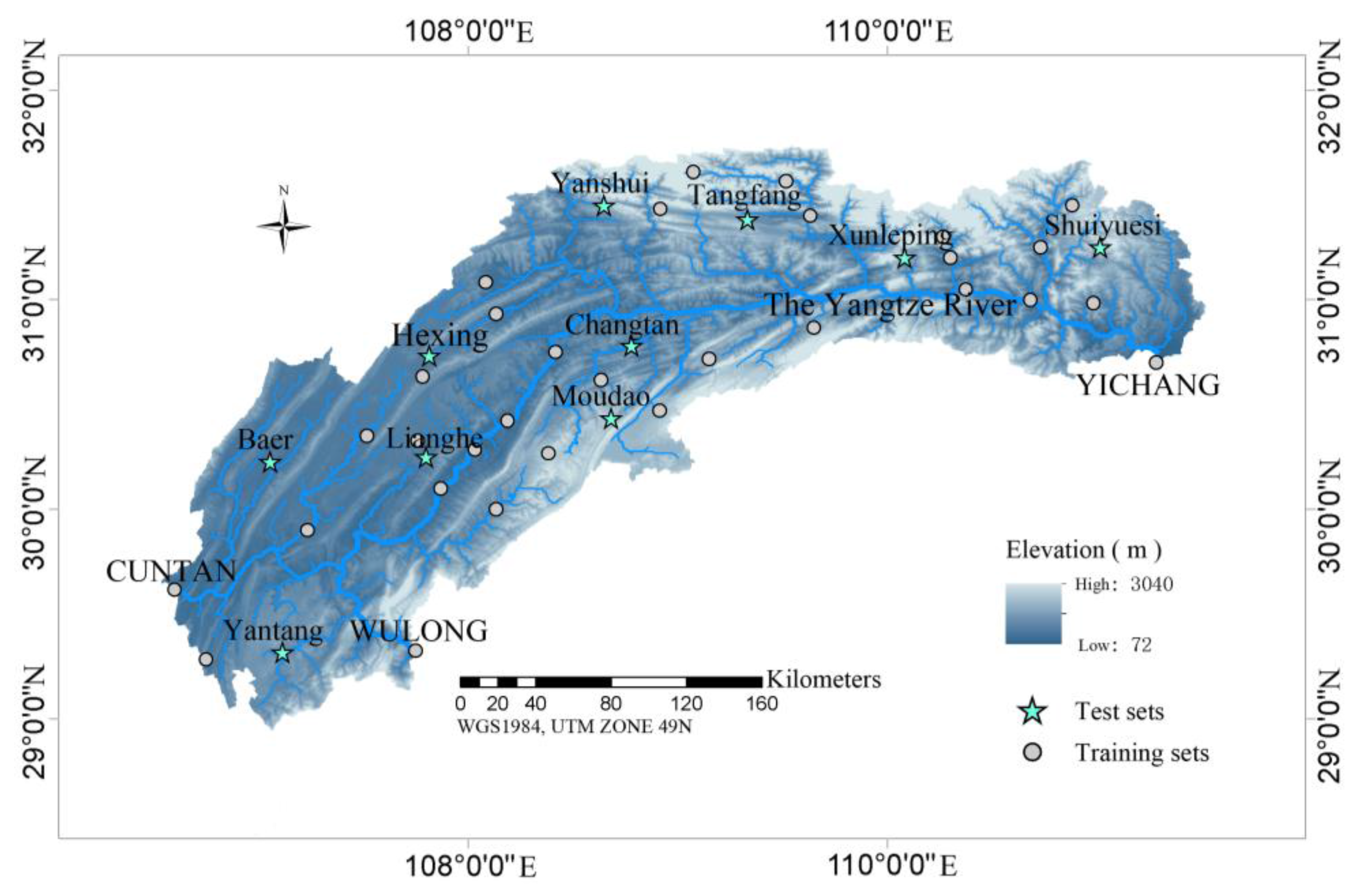
2.1. Research Basin
2.2. Research Data
2.2.1. Ground Observation Data
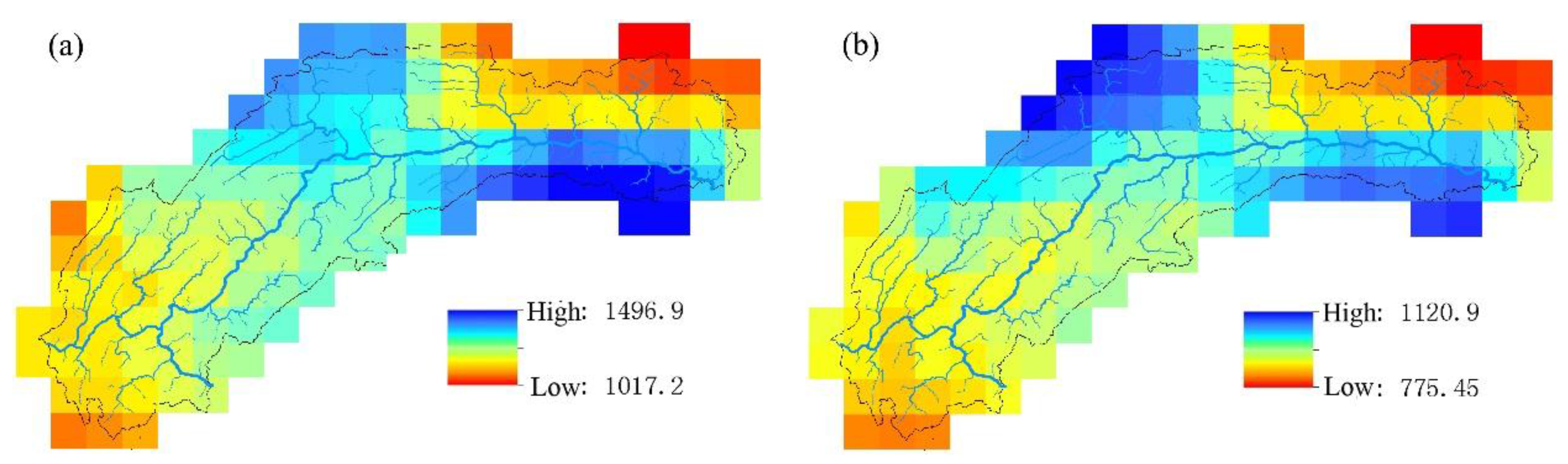
2.2.2. TRMM 3B43 V7 Satellite Precipitation Data
2.3. Interpolation Auxiliary Variable Selection
3. Research Methods
3.1. Commonly-Used Interpolation Methods
3.2. Linear Regression Hybrid Interpolation Method
3.3. Support Vector Machine Interpolation Model
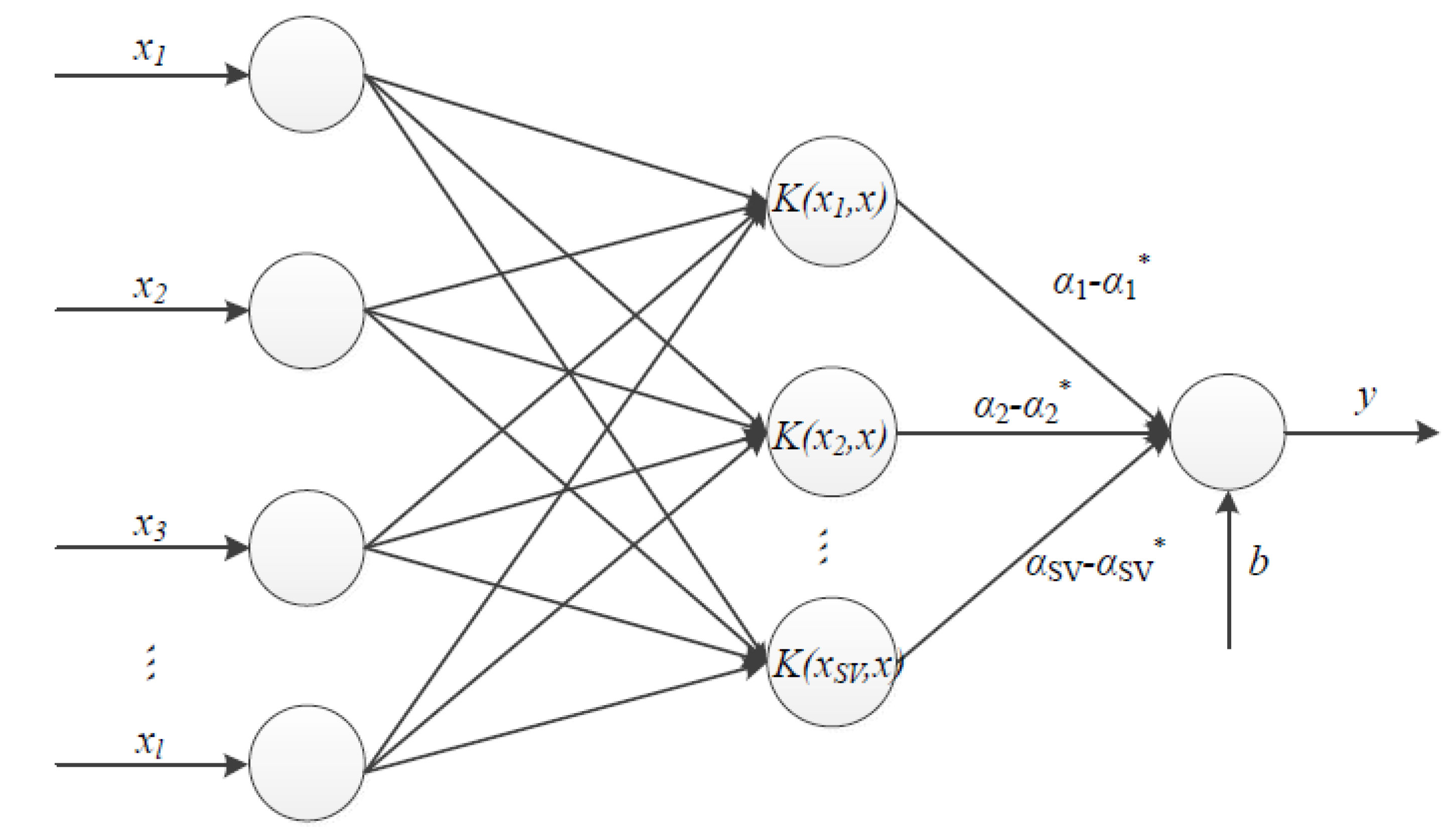
3.3.1. Methodology
3.3.2. Modeling Steps
Input and Output Selection
Data Normalization
Parameter Initialization
Construct a Nonlinear Decision Function
Forecast Based on Nonlinear Decision Function
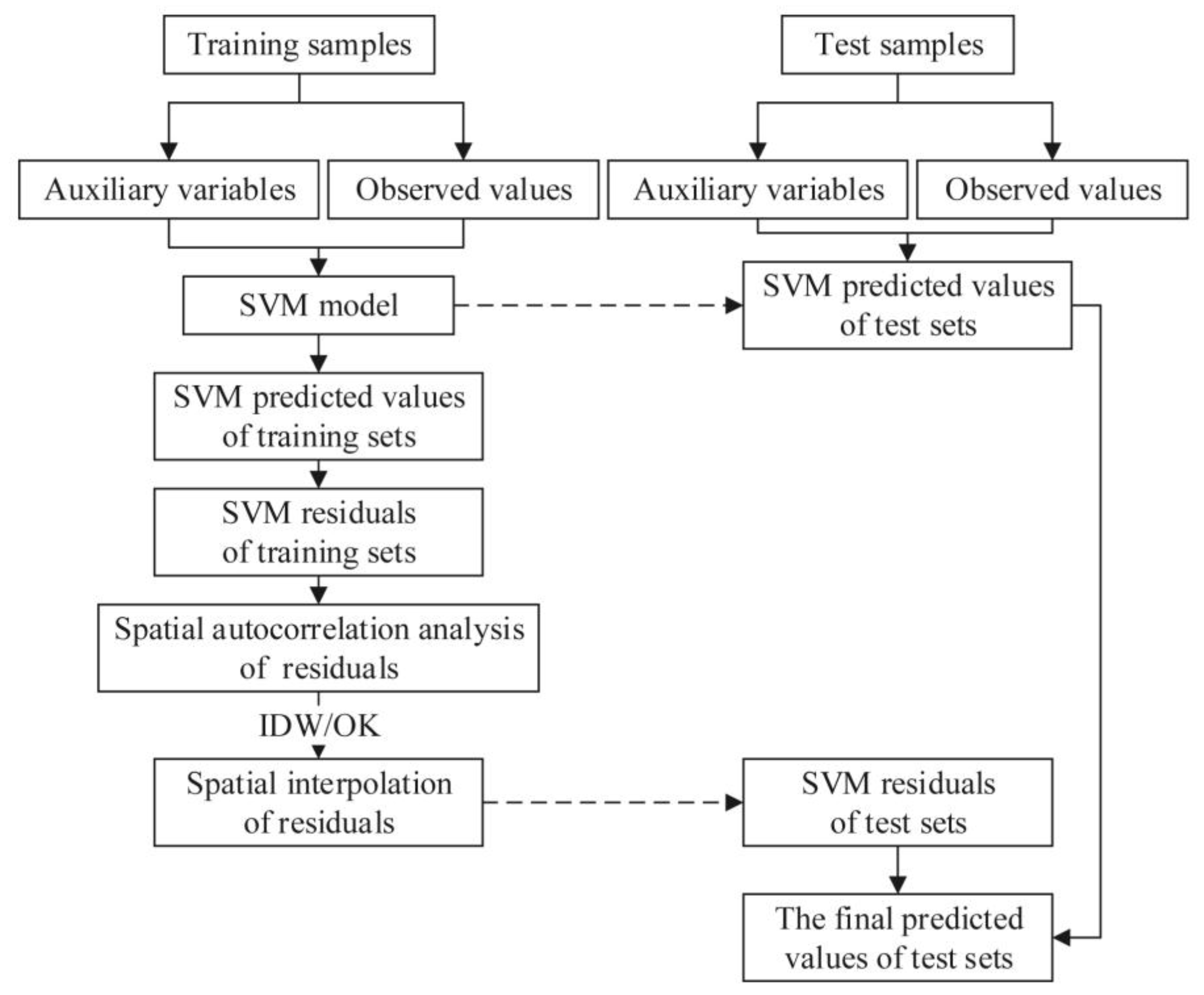
3.4. Support Vector Machine Hybrid Interpolation Method
3.5. Error Evaluation Index
3.5.1. Root Mean Square Error
3.5.2. Mean Relative Error
3.5.3. Coefficient of Determination (R2)
4. Analysis and Discussion of Results
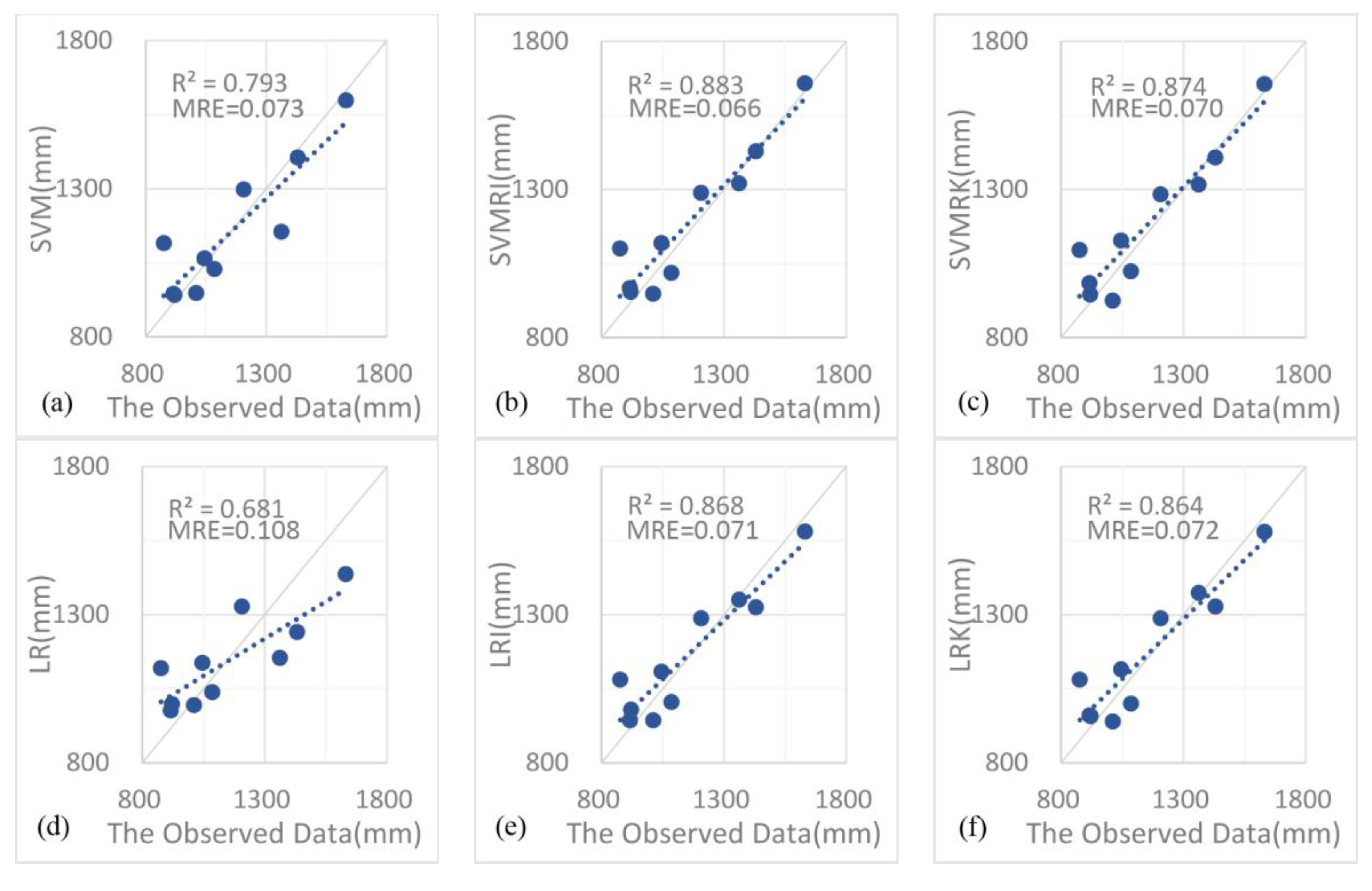
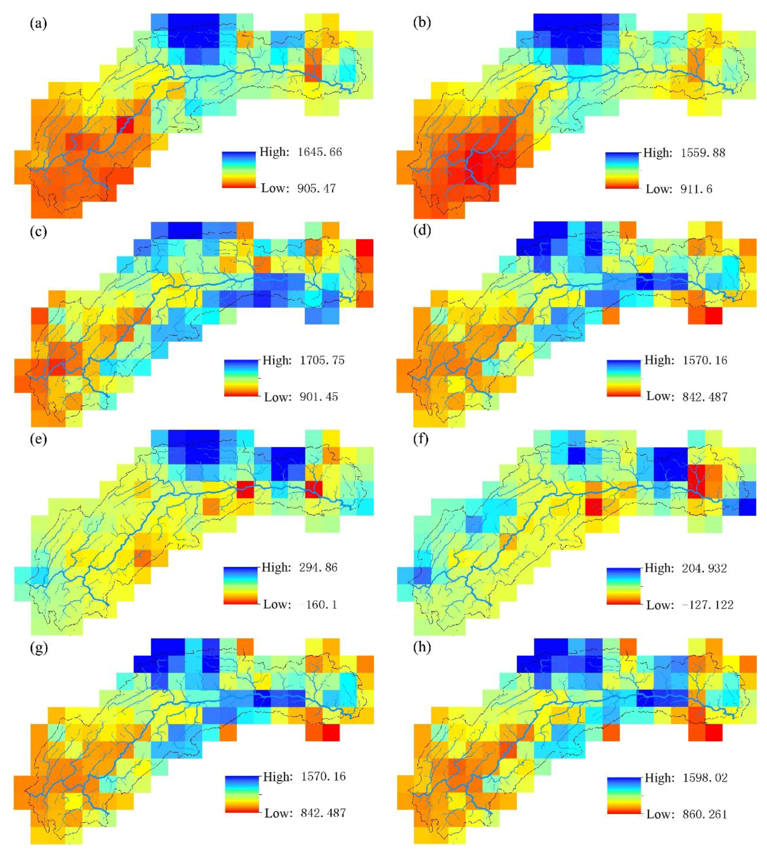
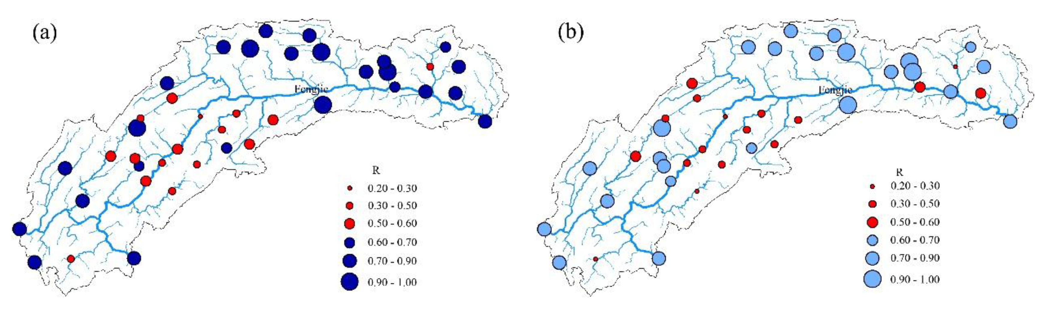
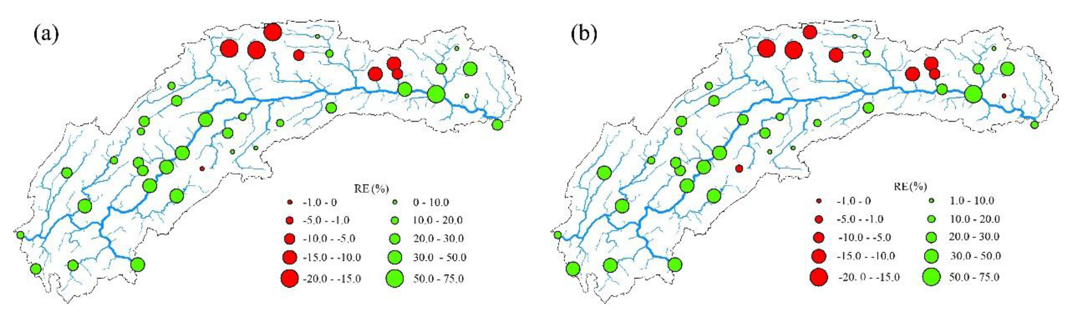
4.1. Results Analysis
4.2. Discussion
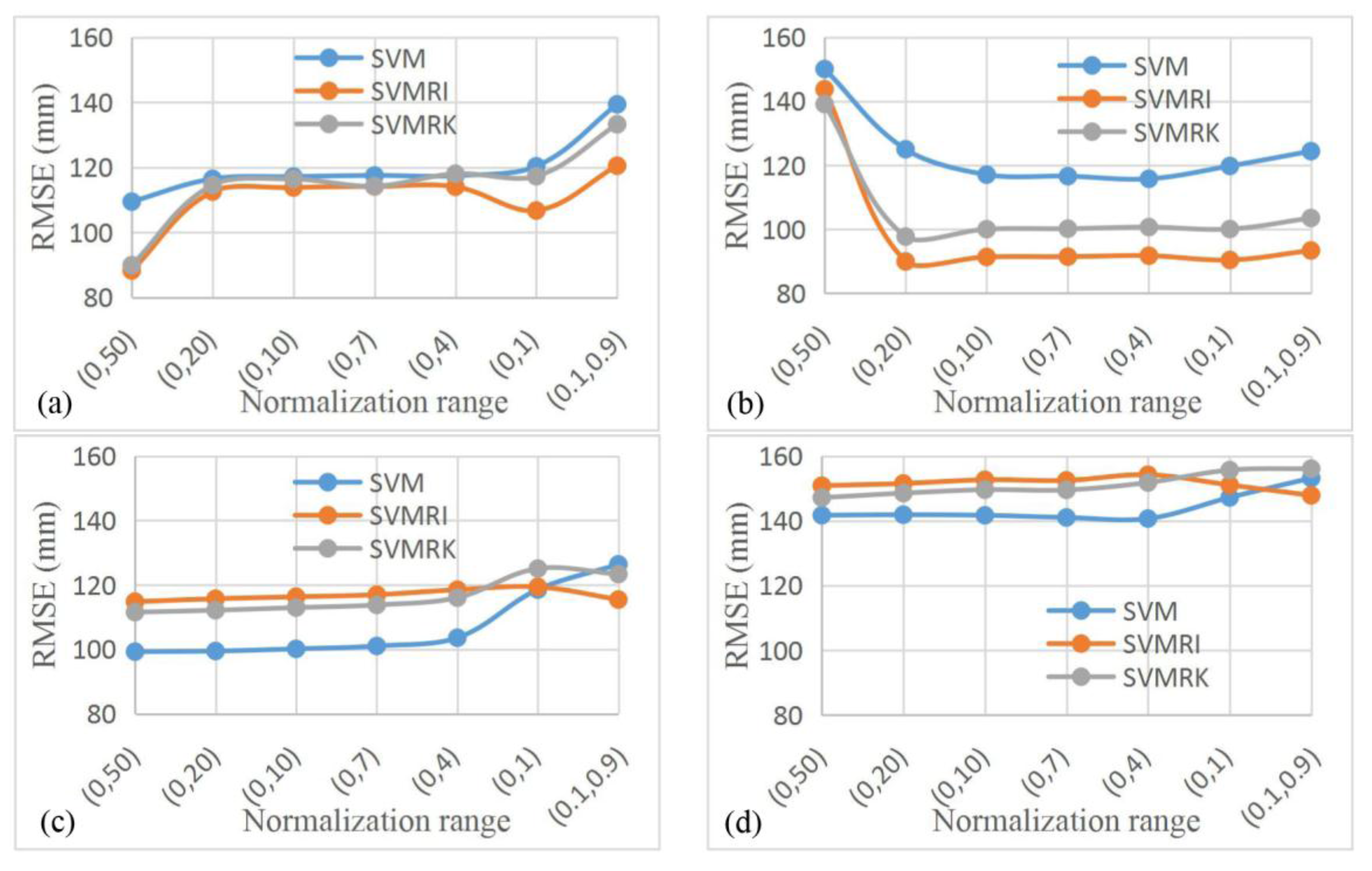
- The insensitive loss parameter , normalization range and other parameters of the SVM model have an impact on the final interpolation results. Rainfall has strong spatiotemporal distribution characteristics, and the rainfall in each region and at each time is not exactly the same, so it is necessary to adjust the parameters according to each set of data. The workload is large and restricted by personal experience and judgment, and the universality of the SVM model needs to be further strengthened.
- The SVM model can well fit the complex nonlinear relationship between the interpolation object and auxiliary variable. After the residual interpolation is superimposed, the prediction accuracy may be improved, or may be reduced, depending on the fitting degree of the SVM model. Choosing a suitable fitting accuracy so that the residuals retain enough precipitation feature information is the key to improving the prediction accuracy of the SVM hybrid interpolation method, but also its chief difficulty.
- Research data were divided into training samples and test samples randomly. During the training phase, SVM could reach the highest forecast accuracy by cross-validation; and in the test phase, the overall error indicator of test samples was used to verify models. Although test samples are random, the verification needs to be richer and more representative. Spatial interpolation calculation of precipitation with multiple time scales and different spatial scopes will result in more scientific and rational conclusions.
5. Conclusions
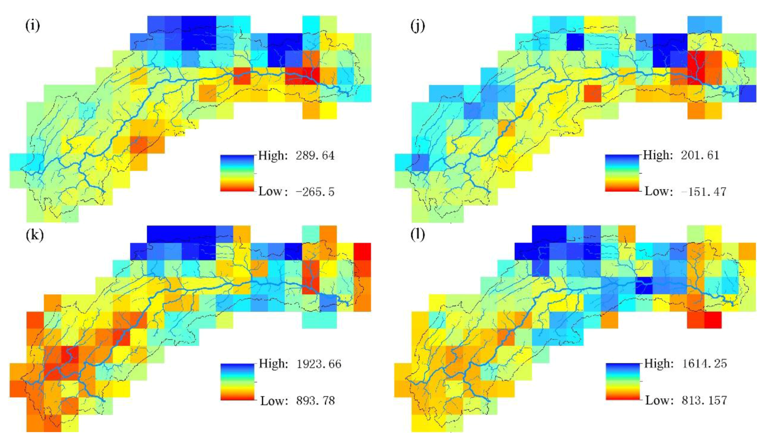
- TRMM 3B43 V7 data deviate from ground site precipitation. Overall, the value is too large, and the rainy center is too small. TRMM data detect the basin precipitation-rich center locations relatively accurately, showing a good spatial distribution continuity, to make up for the shortcomings that the number of local ground sites is insufficient or the distribution is unfavorable. When only the latitude, elevation information and precipitation are used to establish the linear regression equation, the SVM model has poor interpolation precision. Adding the satellite precipitation data as an auxiliary variable significantly improves the interpolation accuracy.
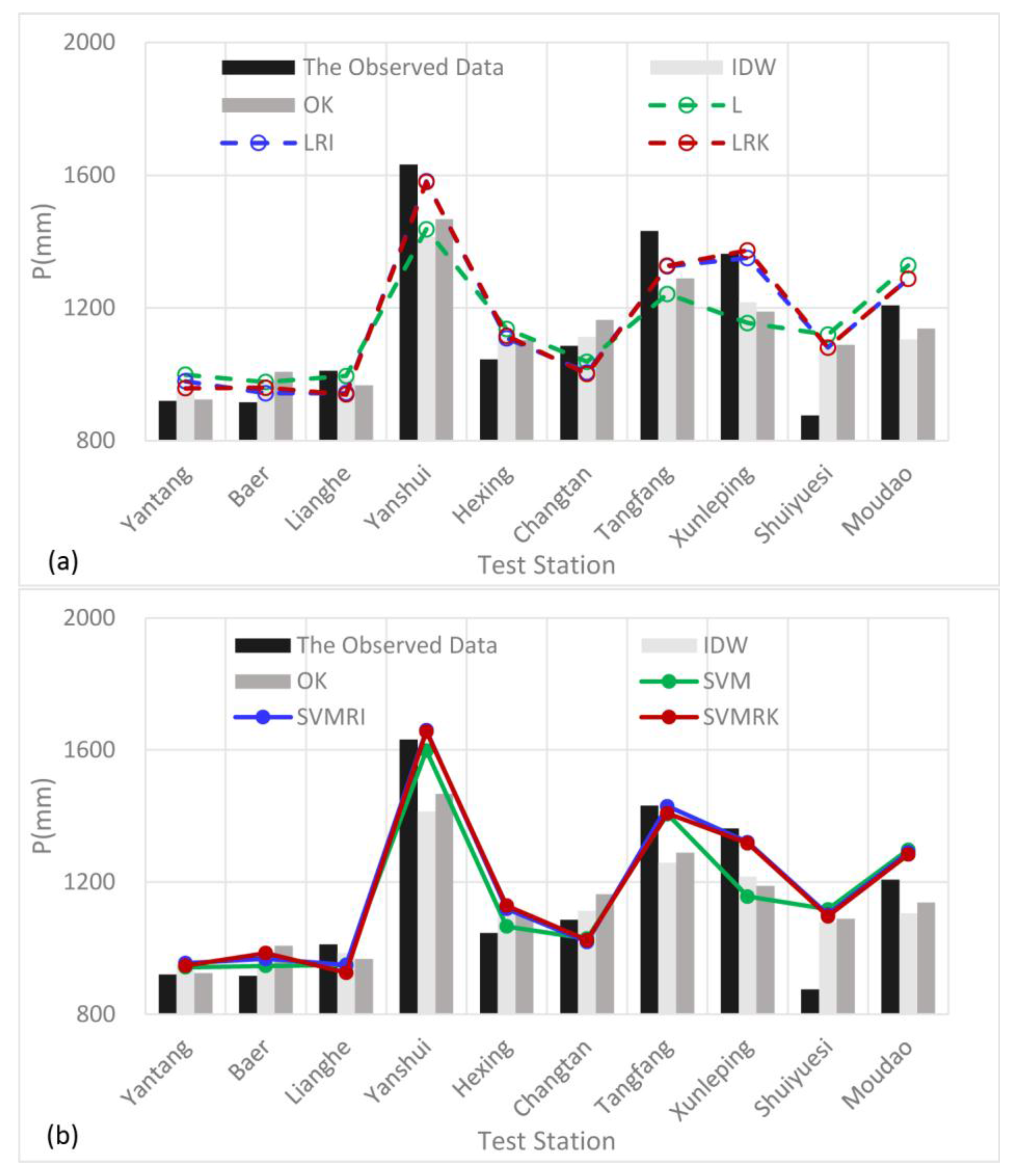
- The support vector machine and SVM hybrid interpolation method obtain better interpolation results than the inverse weight method and ordinary kriging method. The direct predictive result of the SVM model is overall better than that of the linear regression equation. The SVM hybrid interpolation method also obtains better interpolation results than the linear regression hybrid interpolation method.
- The SVM hybrid interpolation method depends on the SVM fitting degree, but it is not the case that the better SVM fits, the higher accuracy the SVM hybrid interpolation method has. The difficult task of choosing a suitable accuracy is the key to improving the prediction accuracy of the SVM.
- The linear regression equation has a greater degree of dependence on the TRMM data than the SVM. The SVM accepts the TRMM data information while maintaining its independence, taking into account that TRMM data linear regression and linear regression hybrid interpolation methods are not suitable for TRMM data evaluation.
Acknowledgments
Author Contributions
Conflicts of Interest
References
- Zhang, J.G.; Xie, P.; Gong, Y.B.; Liu, G.F. Review and perspectives of the research on spatial interpolation of rainfall information. J. Water Res. Water Eng. 2012, 23, 6–9. (In Chinese) [Google Scholar]
- He, H.Y.; Guo, Z.H.; Xiao, W.F. Review on spatial interpolation techniques of rainfall. Chin. J. Ecol. 2005, 24, 1187–1191. (In Chinese) [Google Scholar]
- Li, J.; Heap, A.D. Spatial interpolation methods applied in the environmental sciences: A review. Environ. Model. Softw. 2014, 53, 173–189. [Google Scholar] [CrossRef]
- Lin, J.Y.; Cheng, C.T.; Chau, K.W. Using support vector machines for long-term discharge prediction. Hydrol. Sci. J. 2006, 51, 599–612. [Google Scholar] [CrossRef]
- Asefa, T.; Kemblowski, M.; Mckee, M.; Khalil, A. Multi-time scale stream flow predictions: The support vector machines approach. J. Hydrol. 2006, 318, 7–16. [Google Scholar] [CrossRef]
- Granata, F.; Gargano, R.; de Marinis, G. Support vector regression for rainfall-runoff modeling in urban drainage: A comparison with the EPA’s storm water management model. Water 2016, 8, 69. [Google Scholar] [CrossRef]
- Langhammer, J.; Česák, J. Applicability of a nu-support vector regression model for the completion of missing data in hydrological time series. Water 2016, 8, 560. [Google Scholar] [CrossRef]
- Tripathi, S.; Srinivas, V.V.; Nanjundiah, R.S. Downscaling of precipitation for climate change scenarios: A support vector machine approach. J. Hydrol. 2006, 330, 621–640. [Google Scholar] [CrossRef]
- Chen, S.T.; Yu, P.S.; Tang, Y.H. Statistical downscaling of daily precipitation using support vector machines and multivariate analysis. J. Hydrol. 2010, 385, 13–22. [Google Scholar] [CrossRef]
- Granata, F.; Papirio, S.; Esposito, G.; Gargano, R.; de Marinis, G. Machine learning algorithms for the forecasting of wastewater quality indicators. Water 2017, 9, 105. [Google Scholar] [CrossRef]
- Huang, Z.S.; Wang, H.Z.; Zhang, R. An improved kriging interpolation technique based on SVM and its recovery experiment in oceanic missing data. Am. J. Comput. Math. 2012, 2, 56–60. [Google Scholar] [CrossRef]
- Gilardi, N.; Bengio, S. Comparison of four machine learning algorithms for spatial data analysis. Conf. Signals Syst. Comput. 2009, 17, 160–167. [Google Scholar]
- Li, C.P.; Zheng, Y.X.; Li, Z.X.; Zhao, Y.Q. Modeling and Application of Ore Grade Interpolation Based on SVM. In Proceedings of the 2011 Eighth International Conference on Fuzzy Systems and Knowledge Discovery (FSKD), Shanghai, China, 26–28 July 2011; Volume 3, pp. 1522–1525. [Google Scholar]
- Liu, Y.F.; Li, R.X.; Li, C.B.; Liu, X.N. Application of BP neural network and support vector machine to the accumulated temperature interpolation. J. Arid Land Resour. Environ. 2014, 28, 158–165. (In Chinese) [Google Scholar]
- Feng, Y.M.; Liang, J. Space data fitting based on the support vector machine-SVM. Hydrogr. Surv. Chart. 2009, 29, 31–33. (In Chinese) [Google Scholar]
- Li, J.; Heap, A.D.; Potter, A.; Daniell, J.J. Application of machine learning methods to spatial interpolation of environmental variables. Environ. Model. Softw. 2011, 26, 1647–1659. [Google Scholar] [CrossRef]
- Zhu, L.; Huang, J.F. Comparison of spatial interpolation method for precipitation of mountain areas in county scale. Trans. Chin. Soc. Agric. Eng. 2007, 23, 80–85. (In Chinese) [Google Scholar]
- Sun, W.; Zhu, Y.Q.; Huang, S.L.; Guo, C.X. Mapping the mean annual precipitation of China using local interpolation techniques. Theor. Appl. Climatol. 2015, 119, 171–180. [Google Scholar] [CrossRef]
- Bostan, P.A.; Heuvelink, G.B.M.; Akyurek, S.Z. Comparison of regression and kriging techniques for mapping the average annual precipitation of Turkey. Int. J. Appl. Earth. Obs. 2012, 19, 115–126. [Google Scholar] [CrossRef]
- Seo, Y.; Kim, S.; Singh, V.P. Estimating spatial precipitation using regression kriging and artificial neural network residual kriging (RKNNRK) hybrid approach. Water Resour. Manag. 2015, 29, 2189–2204. [Google Scholar] [CrossRef]
- Kizza, M.; Westerberg, I.; Rodhe, A.; Ntale, H.K. Estimating areal rainfall over Lake Victoria and its basin using ground-based and satellite data. J. Hydrol. 2012, 464, 401–411. [Google Scholar] [CrossRef]
- Tang, G.Q.; Li, Z.; Xue, X.W.; Hu, Q.F.; Yong, B.; Hong, Y. A study of substitutability of TRMM remote sensing precipitation for gauge-based observation in Ganjiang River basin. Adv. Water Sci. 2015, 26, 340–346. (In Chinese) [Google Scholar]
- Tekeli, A.E.; Fouli, H. Evaluation of TRMM satellite-based precipitation indexes for flood forecasting over Riyadh City, Saudi Arabia. J. Hydrol. 2016, 541, 471–479. [Google Scholar] [CrossRef]
- Jiang, S.H.; Zhou, M.; Ren, L.L.; Cheng, X.R.; Zhang, P.J. Evaluation of latest TMPA and CMORPH satellite precipitation products over Yellow River Basin. Water Sci. Eng. 2016, 9, 87–96. [Google Scholar] [CrossRef]
- Yang, Y.C.; Cheng, G.W.; Fan, J.H.; Sun, J.; Li, W.P. Representativeness and reliability of satellite rainfall dataset in alpine and gorge region. Adv. Water Sci. 2013, 24, 24–33. (In Chinese) [Google Scholar]
- Oke, A.M.C.; Frost, A.J.; Beesley, C.A. The use of TRMM satellite data as a predictor in the spatial interpolation of daily precipitation over Australia. In Proceedings of the 18th World IMACS/MODSIM Congress on Modelling and Simulation, Cairns, Australia, 13–17 July 2009; Volume 1, pp. 3726–3732. [Google Scholar]
- Álvarez-Villa, O.D.; Vélez, J.I.; Poveda, G. Improved long-term mean annual rainfall fields for Colombia. Int. J. Climatol. 2011, 31, 2194–2212. [Google Scholar] [CrossRef]
- Wagner, P.D.; Fiener, P.; Wilken, F.; Kumar, S.; Schneider, K. Comparison and evaluation of spatial interpolation schemes for daily rainfall in data scarce regions. J. Hydrol. 2012, 464, 388–400. [Google Scholar] [CrossRef]
- Teng, H.F.; Shi, Z.; Ma, Z.Q.; Li, Y. Estimating spatially downscaled rainfall by regression kriging using TRMM precipitation and elevation in Zhejiang Province, southeast China. Int. J. Remote Sens. 2014, 35, 7775–7794. [Google Scholar] [CrossRef]
- Li, Z. Multi-source Precipitation Observations and Fusion for Hydrological Applications in the Yangtze River Basin. Ph.D. Thesis, Tsinghua University, Beijing, China, 2015. (In Chinese). [Google Scholar]
- Hu, Q.F.; Yang, D.W.; Wang, Y.T.; Yang, H.B. Monthly runoff simulation in Gan river basin using rainfall TRMM 3B43V7. J. Hydroelectr. Eng. 2014, 33, 6–12. (In Chinese) [Google Scholar]
- Tang, G.A.; Yang, X. ArcGIS Geographic Information System Spatial Analysis the Experimental Tutorial (2); Science Press: Beijing, China, 2012. (In Chinese) [Google Scholar]
- Ly, S.; Charles, C.; Degré, A. Different methods for spatial interpolation of rainfall data for operational hydrology and hydrological modeling at watershed scale: A review. Biotechnol. Agron. Soc. Environ. 2013, 17, 392–406. [Google Scholar]
- Vicente-Serrano, S.M.; Saz-Sánchez, M.A.; Cuadrat, J.M. Comparative analysis of interpolation methods in the middle Ebro Valley (Spain): Application to annual precipitation and temperature. Clim. Res. 2003, 24, 161–180. [Google Scholar] [CrossRef]
- Wang, X.C.; Shi, F.; Yu, L.; Li, Y. MATLAB Neural Network Analysis of 43 Cases; Beihang University Press: Beijing, China, 2016. (In Chinese) [Google Scholar]
- Li, M.; Shao, Q.X. An improved statistical approach to merge satellite rainfall estimates and raingauge data. J. Hydrol. 2010, 385, 51–64. [Google Scholar] [CrossRef]
- Sun, L.Q.; Hao, Z.C.; Wang, J.H.; Nistor, I.; Seidou, O. Assessment and correction of TMPA products 3B42RT and 3B42V6. J. Hydraul. Eng. 2014, 46, 1135–1146. (In Chinese) [Google Scholar]
- Pan, Y.; Shen, Y.; Yu, J.J.; Xiong, A.Y. An experiment of high-resolution gauge-radar-satellite combined precipitation retrieval based on the Bayesian merging method. Acta Meteorol. Sin. 2015, 73, 177–186. (In Chinese) [Google Scholar]
- Li, X.; Cheng, G.D.; Lu, L. Comparison of spatial interpolation methods. Adv. Earth Sci. 2000, 15, 260–265. (In Chinese) [Google Scholar]


| Correlation Coefficient | Geographic Location | Terrain Characteristics | Satellite Precipitation | |||||
|---|---|---|---|---|---|---|---|---|
| X | Y | S | A | E | E10 | T | Tfs | |
| Pearson | 0.226 | 0.540 ** | 0.275 | 0.198 | 0.567 ** | 0.610 ** | 0.387 * | 0.528 ** |
| Spearman | 0.338 * | 0.536 ** | 0.271 | 0.383 * | 0.524 ** | 0.552 ** | 0.453 ** | 0.497 ** |
| Dependent Variable | Initial Independent Variable | Independent Variable Removed (Not Significant) | Final Independent Variable (Significant) | Regression Equation (Significant) | |
|---|---|---|---|---|---|
| P | 1 | Y-E-T | T | Y-E | P = −2819.38 + 123.69 × Y + 0.24 × E |
| 2 | Y-E-Tfs | Y | E-Tfs | P = −288.08 + 0.27 × E + 1.39 × Tfs | |
| 3 | Y-E10-T | Y, T | E10 | P = 791.61 + 0.20 × Z10 | |
| 4 | Y-E10-Tfs | Y | E10-Tfs | P = −539.24 + 0.19 × Z10 + 1.40 × Tfs | |
| Method | Test Set RMSE (mm) | Test Set MRE | Test Set R2 | |||||||
|---|---|---|---|---|---|---|---|---|---|---|
| Worst | Mean | Best | Worst | Mean | Best | Worst | Mean | Best | ||
| SVM | Y-E | 262.596 | 252.111 | 231.954 | 0.158 | 0.155 | 0.152 | 0.236 | 0.238 | 0.226 |
| Y-E-T | 139.397 | 119.676 | 109.445 | 0.097 | 0.078 | 0.073 | 0.735 | 0.767 | 0.793 | |
| Y-E-Tfs | 150.120 | 124.128 | 115.792 | 0.110 | 0.086 | 0.079 | 0.633 | 0.746 | 0.770 | |
| Y-E10 | 230.890 | 222.975 | 203.216 | 0.127 | 0.127 | 0.125 | 0.427 | 0.439 | 0.459 | |
| Y-E10-T | 126.379 | 106.926 | 99.289 | 0.089 | 0.072 | 0.068 | 0.757 | 0.811 | 0.831 | |
| Y-E10-Tfs | 153.183 | 143.917 | 140.692 | 0.109 | 0.088 | 0.085 | 0.613 | 0.674 | 0.693 | |
| SVMRI | Y-E-T | 120.502 | 109.988 | 88.255 | 0.092 | 0.079 | 0.066 | 0.801 | 0.830 | 0.883 |
| Y-E-Tfs | 143.777 | 98.873 | 89.958 | 0.106 | 0.076 | 0.071 | 0.673 | 0.835 | 0.865 | |
| Y-E10-T | 119.379 | 116.727 | 114.794 | 0.085 | 0.082 | 0.081 | 0.761 | 0.769 | 0.773 | |
| Y-E10-Tfs | 154.225 | 151.522 | 147.850 | 0.098 | 0.096 | 0.099 | 0.610 | 0.623 | 0.656 | |
| SVMRK | Y-E-T | 133.255 | 114.803 | 89.902 | 0.108 | 0.086 | 0.070 | 0.766 | 0.809 | 0.874 |
| Y-E-Tfs | 139.153 | 105.924 | 97.733 | 0.103 | 0.082 | 0.077 | 0.704 | 0.811 | 0.838 | |
| Y-E10-T | 125.083 | 116.418 | 111.540 | 0.089 | 0.083 | 0.081 | 0.739 | 0.769 | 0.785 | |
| Y-E10-Tfs | 156.121 | 151.206 | 147.150 | 0.105 | 0.095 | 0.088 | 0.626 | 0.631 | 0.645 | |
| L | Y-E | 170.976 | 0.106 | 0.504 | ||||||
| E-Tfs | 145.495 | 0.108 | 0.681 | |||||||
| E10 | 191.842 | 0.116 | 0.488 | |||||||
| E10-Tfs | 145.771 | 0.092 | 0.775 | |||||||
| LRI | Y-E | 108.666 | 0.081 | 0.816 | ||||||
| E-Tfs | 90.303 | 0.071 | 0.868 | |||||||
| E10 | 144.099 | 0.098 | 0.719 | |||||||
| E10-Tfs | 128.143 | 0.085 | 0.768 | |||||||
| LRK | Y-E | 111.001 | 0.087 | 0.796 | ||||||
| E-Tfs | 90.987 | 0.072 | 0.864 | |||||||
| E10 | 147.082 | 0.097 | 0.661 | |||||||
| E10-Tfs | 138.954 | 0.098 | 0.729 | |||||||
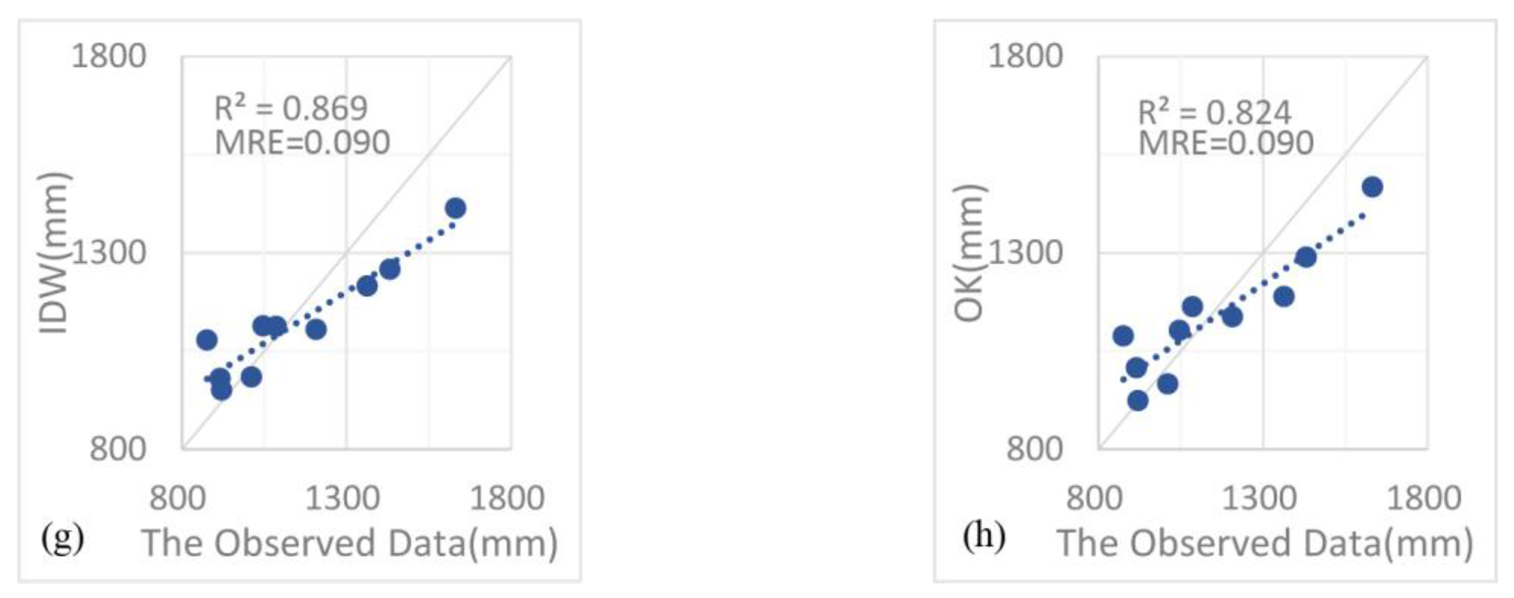
| IDW | 127.092 | 0.090 | 0.869 | |||||||
| OK | 121.424 | 0.090 | 0.824 | |||||||
| Input Vector | SVM Normalization Range | SVMRI Normalization Range | SVMRK Normalization Range | |||
|---|---|---|---|---|---|---|
| The Worst RMSE | The Best RMSE | The Worst RMSE | The Best RMSE | The Worst RMSE | The Best RMSE | |
| Y-E | (0, 50) | (0.1, 0.9) | / | / | / | / |
| Y-E-T | (0.1, 0.9) | (0, 50) | (0.1, 0.9) | (0, 50) | (0.1, 0.9) | (0, 50) |
| Y-E-Tfs | (0, 50) | (0, 4) | (0, 50) | (0, 20) | (0, 50) | (0, 20) |
| Y-E10 | (0, 10) | (0.1, 0.9) | / | / | / | / |
| Y-E10-T | (0.1, 0.9) | (0, 50) | (0, 1) | (0, 50) | (0, 1) | (0, 50) |
| Y-E10-Tfs | (0.1, 0.9) | (0, 4) | (0, 4) | (0.1, 0.9) | (0.1, 0.9) | (0, 50) |
| Support Vector Machine Hybrid Interpolation | Linear Regression Hybrid Interpolation | ||||
|---|---|---|---|---|---|
| Auxiliary Variable | SVMRI | SVMRK | Auxiliary Variable | LRI | LRK |
| Y-E-T | −19.36% | −17.86% | Y-E | −36.44% | −35.08% |
| Y-E-Tfs | −22.31% | −15.60% | E-Tfs | −35.11% | −37.46% |
| Y-E10-T | 15.62% | 12.34% | E10 | −24.89% | −23.33% |
| Y-E10-Tfs | 5.09% | 4.59% | E10-Tfs | −17.92% | −4.68% |
| Index | IDW | OK | LRI | SVMRI |
|---|---|---|---|---|
| Gauge precipitation (mm) | 1085.811 | 1094.046 | 1165.304 | 1109.604 |
| TRMM (mm) | 1267.984 | 1267.984 | 1267.984 | 1267.984 |
| Relative error | 16.78% | 15.90% | 8.81% | 14.27% |
© 2017 by the authors. Licensee MDPI, Basel, Switzerland. This article is an open access article distributed under the terms and conditions of the Creative Commons Attribution (CC BY) license (http://creativecommons.org/licenses/by/4.0/).
Share and Cite
Zhang, X.; Liu, G.; Wang, H.; Li, X. Application of a Hybrid Interpolation Method Based on Support Vector Machine in the Precipitation Spatial Interpolation of Basins. Water 2017, 9, 760. https://doi.org/10.3390/w9100760
Zhang X, Liu G, Wang H, Li X. Application of a Hybrid Interpolation Method Based on Support Vector Machine in the Precipitation Spatial Interpolation of Basins. Water. 2017; 9(10):760. https://doi.org/10.3390/w9100760
Chicago/Turabian StyleZhang, Xiaoxiao, Guodong Liu, Hantao Wang, and Xiaodong Li. 2017. "Application of a Hybrid Interpolation Method Based on Support Vector Machine in the Precipitation Spatial Interpolation of Basins" Water 9, no. 10: 760. https://doi.org/10.3390/w9100760
APA StyleZhang, X., Liu, G., Wang, H., & Li, X. (2017). Application of a Hybrid Interpolation Method Based on Support Vector Machine in the Precipitation Spatial Interpolation of Basins. Water, 9(10), 760. https://doi.org/10.3390/w9100760