Article

Estimating River Depth from SWOT-Type Observables Obtained by Satellite Altimetry and Imagery

Institute of Geodesy, University of Stuttgart, 70174 Stuttgart, Germany
*
Author to whom correspondence should be addressed.
Water 2017, 9(10), 753; https://doi.org/10.3390/w9100753
Submission received: 14 April 2017 / Revised: 8 September 2017 / Accepted: 26 September 2017 / Published: 30 September 2017
(This article belongs to the Special Issue Advances in Hydro-Meteorological Monitoring)

Abstract

:
The proposed Surface Water and Ocean Topography (SWOT) mission aims to improve spaceborne estimates of river discharge through its measurements of water surface elevation, river width and slope. SWOT, however, will not observe baseflow depth, which limits its value in estimating river discharge especially for those rivers with heterogeneous channel geometry. In this study, we aim to obtain river depths from spaceborne observations together with in situ data of river discharge. We first obtain SWOT-like observables from current satellite techniques. We obtain river water level and slope time series from multi-mission altimetry and effective river width from satellite imagery (MODIS). We then employ a Gauss–Helmert adjustment model to estimate average river depth for 16 defined reaches along the Po River in Italy, for which we use our spaceborne observations in two recognized models for discharge estimation. The average river depth estimates along the Po River are validated against surveyed cross-section information, which shows a generally good agreement in the range of ∼10% relative root mean squared error. Furthermore, we analyzed the sensitivity of error in the estimated river depth to errors of individual parameters. We show that the estimated river depth is less influenced by errors of river width and river discharge, while it is strongly influenced by errors in water level. This result gives a perspective to the SWOT mission to infer river depth by coarse estimates of river width and discharge.

1. Introduction

River discharge is perhaps the single most important hydrologic quantity representing the amount of available freshwater on landmasses [1]. Despite its importance, the publicly available in situ river discharge database has been declining steadily over the past few years due mainly to economic and political reasons [2,3,4]. The number of available runoff gauging stations has gone down from about 8000 (pre-1970) to less than 1000 (around the year 2015). Also during this period, the total monitored annual stream flow has dropped accordingly by about 75%. Figure 1 indicates that not only the number of existing stations has decreased, but also in situ measurements over a number of important basins in Africa and South America are no longer available. In fact, most of the active gauges are located over developed countries, and the density of stations is much sparser in the non-industrialized countries [5].
The potential of spaceborne and airborne techniques for obtaining river discharge estimates has been demonstrated by many studies [1,4,6,7,8,9,10,11]. The work in [12] found a power law correlation between satellite-derived effective width and discharge using ERS 1 SAR images and simultaneous ground measurements of discharge. Different models are examined in [9] using satellite-derived hydraulic parameters including water surface width, surface velocity, stage and slope. The research in [13] employed TOPEX/Poseidon altimetry data to estimate river discharge based on a relation between water level and discharge. The study in [14] used a data assimilation technique (ensemble Kalman filter) built around a river hydrodynamic model to recover water depth and discharge. The work in [4] introduced a statistical approach to derive discharge from river height through a rating curve based on quantile functions. At-Many-stations Hydraulic Geometry (AMHG) was proposed in [15] where paired coefficients and exponents of At-a-station Hydraulic Geometry (AHG) from many cross-sections of a given river reach are functionally related to one another, following a log-linear relationship. The study in [16] presents the Metropolis–Manning (MetroMan) algorithm to estimate river bathymetry, the roughness coefficient and discharge based on input measurements of river water surface elevation (H) and slope (s) using the Metropolis algorithm in a Bayesian Markov chain Monte Carlo scheme. The research in [17] implemented a form of Manning’s equation to retrieve the river low flow bathymetry, roughness and discharge ( H 0 , K, Q). The Mean-annual Flow and Geomorphology (MFG) algorithm was introduced in [11], which uses the so-called wide-channel approximation leading to a form of Manning’s equation that approximates river depth as the difference between water surface elevation and the cross-sectional average river bathymetry. Furthermore, Ref. [11] described the Mean Flow with Constant Roughness (MFCR) approach, which assumes a constant value for the roughness coefficient and uses the Water Balance Model (WBM) mean annual flow estimation. Recently, different methodologies were developed to reconstruct a spatially- and temporally-complete estimate of discharge from a set of observations [18,19,20,21]. Moreover, Kalman filters and smoothers have been widely used with river water level data for discharge estimation. The work in [14] assimilated synthetic water elevation observations into a river hydrodynamics model using an ensemble Kalman filter to estimate river discharge. The study in [22] used Kalman filtering to assimilate water level information with simulations from a coupled hydrological and hydrodynamic model to estimate discharge in an ungauged basin scenario. The study in [23] estimated river bathymetry for retrieving river discharge from the Surface Water and Ocean Topography (SWOT) satellite mission using an ensemble Kalman filter-based data assimilation algorithm coupled with a hydrodynamic model. The research in [24] assimilated in situ and radar altimetry data into a large-scale hydrologic-hydrodynamic model for streamflow forecasts in the Amazon.
However, all of these studies are limited to some extent by the characteristics of present-day sensors. The proposed SWOT mission, a joint project between the United States and France, aims to alleviate the limitations and significantly improve spaceborne estimates of river discharge. The SWOT mission will provide measurements of water surface elevation, river width and slope, through which discharge can be estimated for river widths down to 50–100 m [25]. Despite the promising perspective of the mission, one should keep in mind that SWOT will not observe baseflow depth (Figure 2), which limits its value for estimating river discharge especially for those rivers with heterogeneous channel geometry [26]. Therefore, river channel bathymetry is a significant source of uncertainty in estimating discharge from spaceborne measurements [7].
Some recent research was devoted to estimate river depth from currently available remote sensing techniques. The work in [27] assessed the feasibility of mapping fluvial systems with passive optical remote sensing and analyzing the physical processes of radiative transfer in shallow stream channels. A spectrally-based approach was suggested in [28] to retrieve depth from passive optical image data. Further, Ref. [29] developed a Forward Image Modeling (FIM) framework for the remote mapping of river morphology via depth retrieval from passive optical images. The research in [30] used a combination of remote sensing imagery and open-channel flow principles to estimate depths for each pixel in an imaged river, which was called the Hydraulically-Assisted Bathymetry (HAB) model. Moreover, Ref. [31] derived mean reach depth from the parameters of the power law establishing the rating curve between water stages from satellite altimetry. A general relation to estimate the bankfull depth was introduced in [32] from observed width and slope, although with significant error in the estimation. The work in [14] used a data assimilation technique (ensemble Kalman filter) built around a river hydrodynamic model to recover water depth and discharge. Similarly, Ref. [7] estimated bathymetric depth and slope using synthetically-generated SWOT measurements and a Data Assimilation (DA) methodology. The study in [33] combined coupled hydrologic/hydrodynamic modeling of an Arctic river with virtual SWOT observations using a local ensemble Kalman smoother to characterize river depth. An algorithm to obtain estimates of river depth and discharge was developed in [34] based on Manning’s equation, which reduces the computational expense in contrast to data assimilation techniques. Finally, Ref. [26] proposed “linear” and “slope-break” extrapolation methods that seek to identify optimal locations where there is high correlation between w (cross-sectional flow width) or W (effective width) and H (water surface elevation). As they concluded, the slope-break method can detect fewer optimal locations, even though it shows fewer errors than the linear method. Recently, Ref. [35] estimated discharge and as a by product bathymetry based on variational data assimilation using data of water levels and width.
However, none of the aforementioned studies used real spaceborne observations of both water level and river width at the same time to estimate river depth. In this paper, we aim to obtain the river depth using SWOT-type spaceborne observations: water surface elevation (H), effective river width (W) and slope (S). To this end, we use satellite altimetry data for H and S and satellite imagery for the estimation of W. We use our spaceborne observations in two recognized models for discharge estimation developed by Bjerklie [9] and Dingman and Sharma [36]. Since river depth is an unknown in these models, we employ a Gauss–Helmert adjustment model to estimate average river depth along 16 reaches defined over the Po River in Italy. We validate our results against surveyed cross-section information along the river.

2. Case Study

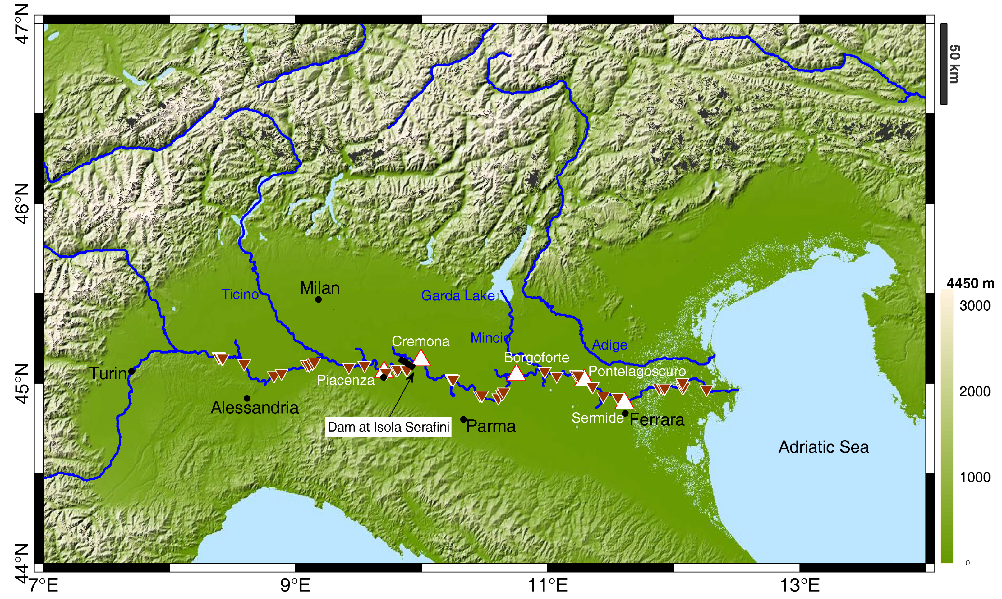
The Po River, located in the Po valley in Italy, flows 652 km eastward through many important Italian cities, including Turin (Torino), Piacenza and Ferrara (Figure 3). Since the river is subject to heavy flooding, over half its length is controlled with dikes. A major dam is located at the village of Isola Serafini 40 km downstream of Piacenza [37]. For this study, we defined 16 reaches along the river from Bressana ( 45.11 ° , 9.12 ° ) up to Berra ( 44.98 ° , 11.98 ° ) almost every 20 km (Table 1). In order to obtain two distinct reaches up and downstream of the dam at Isola Serafini, Reach 5 ends at the dam with a length of 11.8 km, and Reach 6 starts from the dam location with a length of 28.2 km. The river reaches are delineated in Figure 3. We selected this river for this study because of the following reasons.
  • The Po River with its narrow width (150–650 m) highlights the limitations of both altimetry and imagery.
  • We have access to a variety of in situ data for the validation purposes.

3. Data

In this study, we obtained river water level and width from spaceborne sensors. We use the data from different altimetry missions: TOPEX/Poseidon, ENVISAT, CryoSat-2 and the satellite with ARgos and ALtiKa instruments (SARAL/ALtiKa), to generate water level time series along the river. In order to obtain river width, we use MODIS surface reflectance eight-day composites with 250 m spatial resolution (MOD09Q1). We also use in situ data of river discharge for the estimation of river depth and surveyed cross-section information for the validation. Table 2 lists all the data used in this study.

3.1. In Situ Data

In situ datasets at five gauging stations along the Po River are available from from 1995–2013. Table 3 lists the location, elevation, average width, average flow velocity and annual discharge at these gauging stations.
Moreover, we have access to channel section surveys at approximately 250 m intervals between Busca Tornello and the outlet of the river (350 km). These data are provided by Agenzia Interregionale Fiume Po (AIPO).

3.2. Water Level from Satellite Altimetry

With the help of virtual stations and the method defined in [39] (see Table 3 in [39]), individual water level time series along the Po River are densified. That geodetic method allows us to connect hydraulically and statistically all virtual stations of several satellite altimeters and produce water level time series at any location along the river. Here, we generate densified altimetric water level time series at the location of each selected reach. For that, we stacked the selected altimetric measurements by shifting the water level hydrographs of all the virtual stations according to a corresponding time lag. The time lag represents the time that the stream flows from one virtual station to the one downstream. For the time lag estimation, which is necessary for stacking the altimetric measurements, we used average river width W ¯ obtained from satellite images (explained in Section 3.3) together with the average slope S ¯ derived from satellite altimetry as inputs for a hydraulic model that estimates average flow velocity from the width and slope of a river [39]:
V = 1.48 · W ¯ 0.8 S ¯ 0.6 ,
in order to compute the time lag, we then estimate the wave traveling time T L by [6,40]:
T L = L c
in which L is the distance between virtual stations and c is the celerity. In the case of the kinematic wave equation, the momentum balance can be arranged using the Manning formula, and consequently, the celerity c can be expressed as [41]:
c = 5 / 3 V ,
We derive average flow velocity values at each virtual station using Model (1), the estimated river width using imagery and river slope from the average water level of each virtual station. After estimating the time lag and stacking the measurements, the following algorithm is performed to densify the time series:
  • Normalization of the data between zero and one: The measurements are merged by normalizing the time series according to their statistical characteristics. This step helps to make the range for the distribution of water level variations at different virtual stations consistent. For the merging process, the data of each virtual station is normalized by assigning the third percentile to zero and the 85th percentile to one.
  • Confidence limit definition of 99% of a Student’s t-test for a sliding time window: The length of the time window can be experimented with to achieve the best performance. Here, a time window of one month (15 days before and 15 days after the selected measurement) is chosen as it leads to optimal results in terms of time series behavior and the number of identified outliers.
  • Outlier identification and rejection: The identification and the rejection of the outliers is carried out by an iterative data snooping method and by iteratively updating the confidence limits. The data snooping method searches for the observation (always one observation) with the largest gross error [42].
  • Rescaling of normalized values to their corresponding river water level heights: After removing the outliers, the combined normalized altimetric values are ready to be rescaled back to their true water level values.
  • Constructing the time series: After rescaling, we now have a cloud of measurements with their corresponding uncertainty for the selected location along the river, which is free from outliers. The dense time series of water level can then be obtained by connecting the measurements using a three-point distance weighted moving averaging.
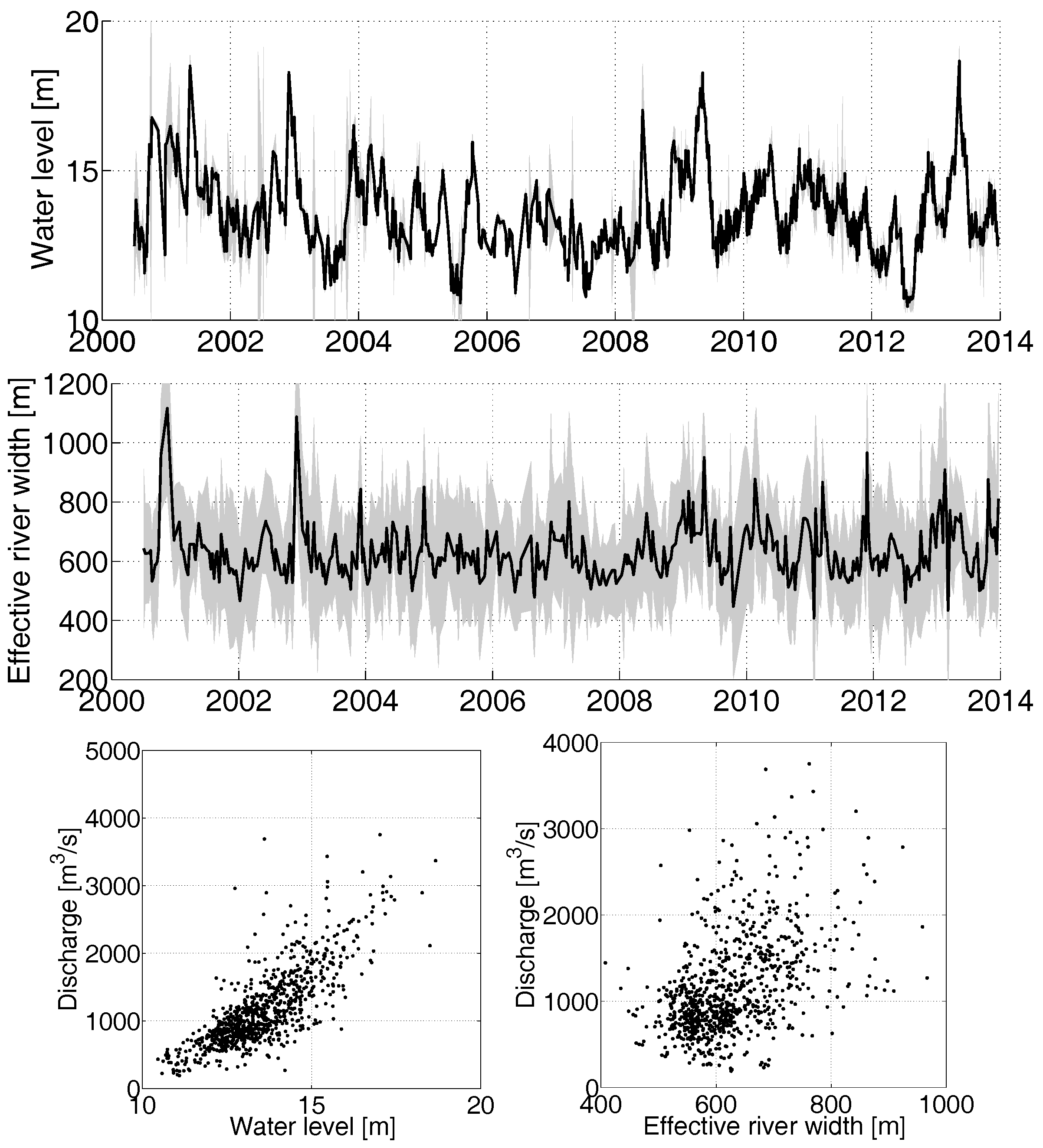
Following the above algorithm, for the densified time series at the all 16 reaches, we obtain an effective temporal resolution of around three days from individual time series with originally a 10- or 35-day sampling interval. Time series in the Figure 4 show the densified water level and effective river width measurements obtained over the reach number 12 (the Borgoforte gauging station).

3.3. River Width from Satellite Imagery

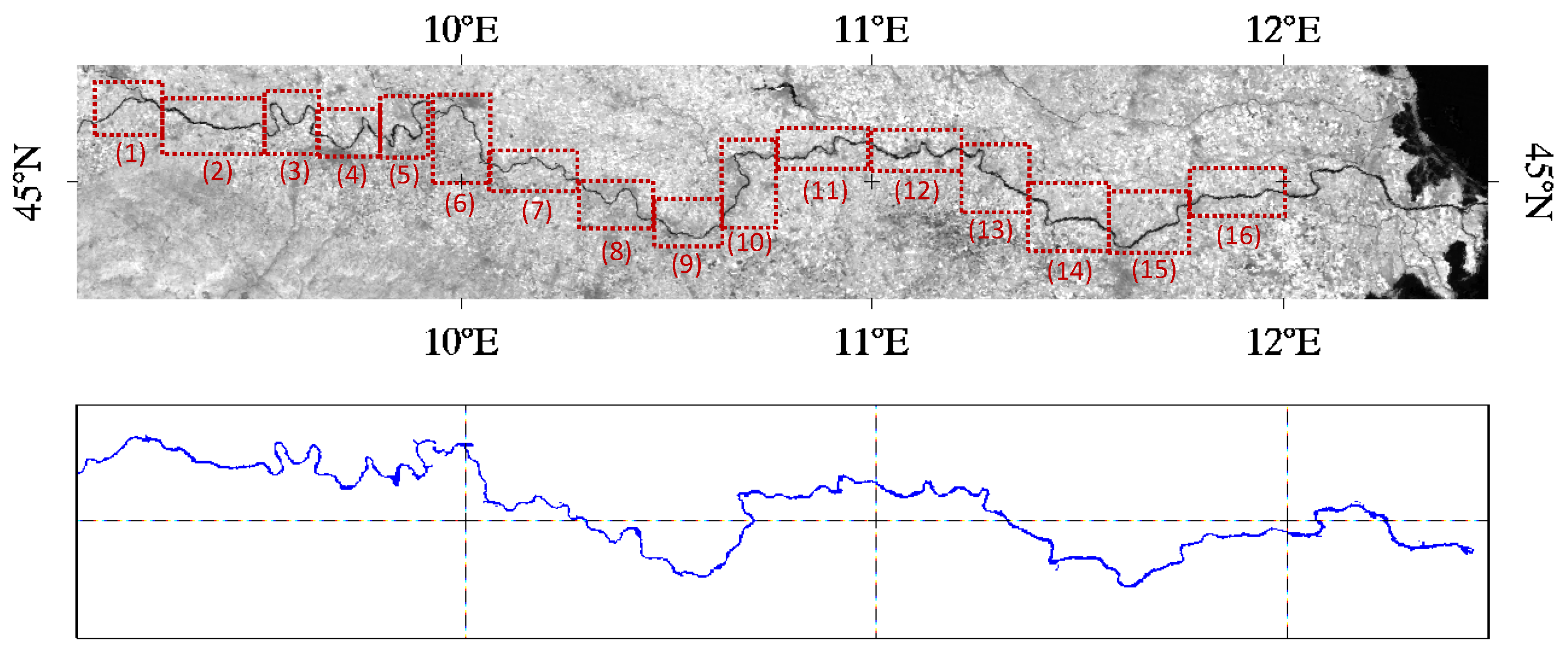
In order to derive the effective width (W) at different river reaches, we apply the algorithm introduced by [38] on MODIS images. The work in [38] developed a Markov Random Fields (MRF) model, which considers spatial correlation between neighboring pixels and the long-term temporal behavior of the river. In this method, to extract the river mask in each image, we define the Maximum A Posteriori (MAP) estimate of the MRF that models the interaction between different constraints and auxiliary sources of information. Based on Bayes’ rule, the posterior probability ( P ( d | f ) ) of the hypothesis f (labeling structure) given the observations d (pixel values) is proportional to the product of the prior probability ( P ( f ) ) and the likelihood ( P ( f | d ) ). In this case, the likelihood represents the agreement between the label and value of pixels, and the prior probability describes the priority between different hypotheses. Our aim is to find a realization of the MRF maximizing the posterior probability. In this way, an energy minimization frame is developed regarding the problem and solved by the graph cuts technique, which is a powerful solution for a wide range of image segmentation problems. We followed the approach by [38] and used an undirected graph with two terminals to extract the river mask by finding the max-flow solution on the graph. Figure 5 presents an example of a derived water mask. It shows that the method is able to continuously capture meandering river paths even for a narrow river like the Po.
Although the graph cuts technique is preferred because of its ability to find a globally-optimal solution in polynomial time, it cannot provide any uncertainty measurement associated with the determined river mask. To overcome this deficiency, Ref. [43] introduced a method to measure uncertainty in graph cuts solutions by measuring the max-marginal probability for each pixel. In this way, a probabilistic river mask can also be provided. Following this, a reliable river area time series is generated together with its uncertainty. We retain the assigned labels for pixels with marginal probabilities higher than 10% in both water and land masks. This leaves a third region that contains pixels with marginal probabilities less than 10% in both masks. This is the uncertain region, for which we cannot define a proper label based on the available information. We consider the area of the third region as an error in river area measurement.
Figure 4 shows the time series of effective river width together with the estimated uncertainty for Reach 12. Since the river is very narrow with respect to the MODIS pixel size of 250 m, the magnitude of uncertainty is relatively large. In Figure 4 (bottom panel), we compare the obtained effective river width against in situ discharge for the same reach. An agreement between the behavior of the two time series is expected. The majority of the river section passes through urban areas with river channel contraction at the shoreline leading to the non-natural behavior of the river. Figure 4 (bottom panel) comprises the obtained water level and the effective river width with the in situ discharge data at Borgoforte. The scatter plots clearly demonstrate the challenge of using satellite imagery for discharge estimation, whereas water level from altimetry agrees relatively well.

4. Methodology to Estimate River Depth

In order to estimate the riverbed’s height H 0 and, consequently, river depth H H 0 , we rely on two models developed for discharge estimation. It should be noted that H 0 is the average riverbed’s height that does not correspond to the height of deepest location in the channel section (see Figure 2). Generally, a functional relationship between depth and discharge can be developed from the Manning equation, which is applicable to natural rivers [44]. For a wide rectangular channel with W > 10 ( H H 0 ) , discharge can be obtained from the Manning equation as:
Q = 1 n ( H H 0 ) 1.67 W S 0.5 ,
in which n is the channel resistance. In practice, the channel resistance cannot be measured directly and often varies considerably with discharge [9]. However, statistical studies by [9,36] have shown that reasonably accurate estimates of discharge Q for within-bank flows can be obtained without resistance as an input variable. The main assumption behind these studies is that the resistance varies with the channel geometry. The works in [9,36] show that discharge can be estimated as:
Bjerklie et al. [9],
Q = a W 1.02 ( H H 0 ) 1.74 S 0.35
Dingman & Sharma [36],
Q = a W 1.17 ( H H 0 ) 1.57 S 0.34
for a wide range of rivers. These models are calibrated using a large database of observed flow measurements from 103 rivers in the United States and New Zealand.
For the estimation of the riverbed’s height H 0 , we have considered both Models (5) and (6). To this end, we use the estimated river width W from satellite imagery, densified altimetric height H, slope S from satellite altimetry and river discharge Q from in situ data. When all these parameters are available, only the H 0 remains as unknown. However, estimating H 0 in such non-linear models, in which different datasets bring different levels of uncertainty, needs extra care. In fact, considering the stochastics of Figure 4 (bottom left), the estimation of H 0 would mean finding the water level (H) where no water passes through the channel ( Q = 0 ) with the added complexity of further stochastic parameters. From the point of view of adjustment, this is an ill-posed extrapolation of data with uncertainties in both axes. Since the data of both axes are provided with uncertainty, standard regression with least squares estimation does not lead to a meaningful H 0 . Therefore, we derive the H 0 , and consequently river depth, by implementing a Gauss–Helmert Model (GHM). Adjustment with the GHM [45] is a combination of adjustment with condition equations and adjustment with observation equations [46].
In the GHM, we add four terms, e Q , e W , e H , e S , to Equations (5) and (6), representing the error in discharge, river width, water level and slope, respectively. Hence, Equation (5) would lead to:
Q e Q a ( W e W ) 1.02 ( H e H H 0 ) 1.74 ( S e S ) 0.35 = f ( a , H 0 , e Q , e W , e H , e S , Q , W , H , S ) = 0 .
We now have an implicit functional relationship f ( . ) linking unknown parameters a , H 0 , e Q , e W , e H , e S to observations Q , W , H , S . We can linearize the function by splitting up the quantities:
H 0 = H 0 0 + δ H 0 , a = a 0 + δ a e W = e W 0 + δ e W , e H = e H 0 + δ e H e S = e S 0 + δ e S , e Q = e Q 0 + δ e Q
and choose Taylor points related to both parameters and uncertainties: a 0 , H 0 0 , e Q 0 , e H 0 and e S 0 . Linearization around these Taylor points yields:
f = f | 0 + f a | 0 δ a + f H 0 | 0 δ H 0 + f e Q | 0 ( e Q e Q 0 ) + f e H | 0 ( e H e H 0 ) + f e S | 0 ( e S e S 0 ) + f e W | 0 ( e W e W 0 ) .
After reshaping, one obtains:
f = f 1 | 0 f 1 e Q | 0 e Q 0 f 1 e H | 0 e H 0 f 1 e S | 0 e S 0 f 1 e W | 0 e W 0 f m | 0 f m e Q | 0 e d 0 f m e H | 0 e H 0 f m e S | 0 e S 0 f m e W | 0 e W 0 w m × 1 + f 1 a | 0 f 1 H 0 | 0 f m a | 0 f m H 0 | 0 A m × 2 δ a δ H 0 δ x 2 × 1 + f 1 e Q | 0 f 1 e H | 0 f 1 e S | 0 f 1 e W | 0 0 0 0 0 0 0 0 0 0 0 0 0 f 2 e Q | 0 f 2 e H | 0 f 2 e S | 0 f 2 e W | 0 0 0 0 0 0 0 0 0 0 0 0 0 f m e Q | 0 f m e H | 0 f m e S | 0 f m e W | 0 B T m × 4 m δ e Q 1 δ e H 1 δ e S 1 δ e W 1 δ e Q m δ e H m δ e S m δ e W m δ v 4 m × 1 = 0
Then, we have the linearized version of (7):
w + A δ x + B T δ v = 0
The upper indices 1, 2, …, m in matrix B T and vector δ v are an index to the observations of discharge, river width, water level and slope. In this formulation, we have two global parameters a, H 0 and 4-m parameters to be estimated from m epochs of { Q i , H i , S i , W i } . In the GHM, the least squares objective function is:
δ x ^ = argmin δ v T P δ v , subject to the Equation ( 11 ) ,
where P is the weight matrix with dimension 4 m × 4 m:
P = diag 1 / σ Q 1 2 , 1 / σ H 1 2 , 1 / σ S 1 2 , 1 / σ W 1 2 , , 1 / σ Q m 2 , 1 / σ H m 2 , 1 / σ S m 2 , 1 / σ W m 2 .
The main benefit of the GHM lies within the weight matrix, which the uncertainties of different measurements carefully take into account. For minimizing Equation (12), the corresponding Lagrangian reads:
L ( v , δ x , λ ) = 1 2 δ v T P δ v λ T ( B T δ v + A δ x + w ) ,
Setting the gradients of the Lagrangian with respect to δ v , δ x , λ to zero yields the equation system:
P 0 B 0 0 A T B T A 0 δ v ^ δ x ^ λ ^ = 0 0 w
by solving Equation (15), we obtain δ x ^ , δ v ^ and λ ^ as:
δ v ^ = B ( B T P B ) 1 { w A [ A T ( B T P B ) 1 A ] 1 A T ( B T P B ) 1 w }
δ x ^ = [ A T ( B T P B ) 1 A ] 1 A T ( B T P B ) 1 w
λ ^ = ( B T P B ) 1 { w A [ A T ( B T P B ) 1 A ] 1 A T ( B T P B ) 1 w } ,
which we can use to update and estimate a ^ , H 0 ^ , e Q ^ , e H ^ , e S ^ and e W ^ . We then update unknown parameters and observations and iterate the whole until convergence is achieved for the norm of δ x ^ and δ v ^ (< 10 9 ). After the final iteration, we obtain a and H 0 with their uncertainties, for which uncertainties of water level, river width, slope and discharge are taken into consideration.

5. Results, Validation and Discussion

Solving the models by [9,36] with the Gauss–Helmert formalism allows us to estimate two unknown parameters of these models namely a and H 0 . For the implementation of the method, we need data of water level (H), slope (S), river width (W) and river discharge (Q). As described in Section 3, we obtain water level time series after applying the densification process [39] over the selected virtual station along the river. Thus, we obtain a water level time series at the middle of each reach, from which we estimate the corresponding time variable slope. The effective river width is obtained from satellite imagery following the method proposed by [38].
In order to fill the weight matrix P, in the Equation (13), we obtain σ H i from satellite altimetry (error envelope in Figure 4 top); σ W i are taken from the error estimation of our effective river width estimation (error envelope in Figure 4 middle); and σ S i are obtained by the error propagation of consecutive height measurements:
σ S i 2 = 1 d 2 ( σ H i up 2 + σ H i do 2 ) ,
in which d is the distance between the center of two consecutive reaches. For σ Q i , we consider 10% of Q measurements, i.e., σ Q i = 0.1 Q i .
Unlike H, W and S that are available for each reach, discharge data are not individually available for each reach. We use discharge data at five in situ gauges along the river. However, the question remains which in situ discharge data lead to a better result for the estimation of H 0 . The intuitive answer to this question is, of course, the discharge data at the gauge nearest to the selected reach. In order to assess this issue, we first estimated H 0 and a for all the reaches with the help of discharge data at all the gauges. Figure 6 shows the estimated H 0 after the implementation of the GHM for the selected reaches along the Po River. For each reach, we obtain five estimates of H 0 ^ and a ^ , for which we use different discharge data. It is interesting to observe that the estimated H 0 for each reach is nearly independent of the choice of discharge data. In principle, we obtain similar values with a discrepancy of ∼2% with respect to average riverbed’s height with the discharge data of different gauges. Comparing the estimated H 0 with those surveyed along the river (black steps) shows a general good agreement in the range of ∼10% relative RMSE.
Such a good agreement is better visible in the scatter plot of estimated H 0 versus in situ H 0 (Figure 7). The scatter is aligned around the diagonal line indicating a good performance of our method for river depth estimation. The results show a marginal difference between the estimated H 0 from the two models, with slightly better performance of the model by [9] (Table 4). As expected, the estimated a ^ values, which act like scale factors, are different for both models. The difference is due to the different power for water level, slope and width data. It should be noted that the unit of value a is also different for the two models. In the case of the model by [9], the unit of a is m 0.24 s 1 , and in the case of the model by [36], it is m 0.26 s 1 .
In order to investigate the impact of the length of time series on the result, we arbitrarily consider 20%, 40%, 60%, 80% and 100% of data in the time series of water level, width and discharge. Figure 8 shows the estimated H 0 for all reaches, where the results of using different portions of datasets for the estimation of H 0 are very similar to each other and lie within the estimated error. This result shows that the estimation of H 0 is insensitive to the length of the time series.
As a result of GHM, δ v ^ is also estimated, which comprises the corrections to the original observations. Figure 9 shows estimated residuals for discharge e Q ^ , water level e H ^ and effective river width e W ^ data of Reach 1 in the case of using the model by [9]. In fact, the two global unknowns of a and H 0 are estimated by adjusting the observations within the selected model and minimizing the error.
Despite good agreement for most reaches, the estimated H 0 for Reaches 4, 7, 8, 12, 15 and 16 show relatively large errors, which can be better seen in Figure 10.
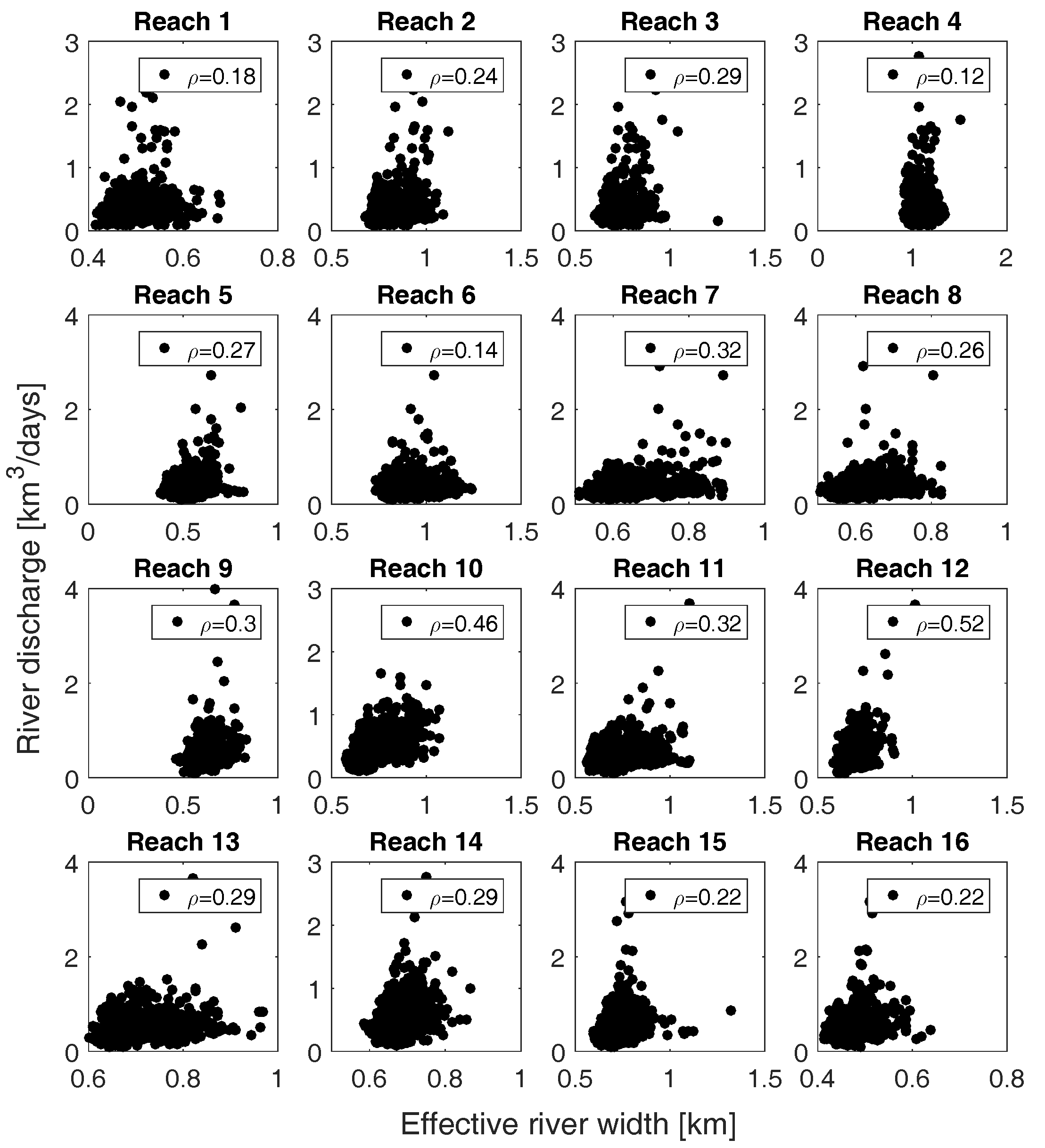
The errors seem to be independent of the choice of the in situ gauge for discharge data. Table 4 lists the results of H 0 estimation for both of the models [9,36], for which we use the discharge data of the nearest in situ station to the reach. It should be noted that for Reaches 1–5, located upstream of the dam, we use the discharge data at a station also located upstream of the dam. The reason for that was the difference between stream behavior up- and down-stream of the dam, which was discussed in detail by [39]. A possible reason for such large errors is the quality of water level or river width time series at these reaches. The water level time series show generally good correlation (>0.6) with discharge data (Figure A1 in Appendix A), and no specific mismatch is visible at the problematic reaches. On the other hand, the correlation coefficients of effective river width with discharge data for all reaches are generally small especially at Reaches 1, 4 and 6 (Figure A2 in Appendix A). However, again, the reaches with a large error for the estimated H 0 do not show a distinctly low correlation in comparison to other reaches. Based on these results, one can conclude that such large errors in estimated H 0 could be due to the choice of the model. In fact, for heterogeneous reaches with variable channel resistance along the river, a single model does not represent the flow over the entire reach.
The error we obtain for the estimated H 0 originated from different sources. Our error assessment should distinguish between systematic errors, accuracy and the precision of our estimation. The systematic error and accuracy in our case are mainly related to the choice of functional model for depth estimation. This is, of course, testable by using different models and by assessing its effect on the estimation of H 0 . In our study, since both models are very similar, we have obtained similar results. In order to assess the sensitivity of estimated H 0 to the precision of W, H and S, we write H 0 as an explicit function of all other parameters (in the case of model by Bjerklie et al.):
H 0 = H Q a W 1.02 S 0.35 0.57 ,
and obtain its error d H 0 as a function of error in other variables:
d H 0 = d H + H 0 Q d Q + H 0 W d W + H 0 S d S ,
in which H 0 / H = 1 , which means that any error in H will directly transfer into an equal error in H 0 .
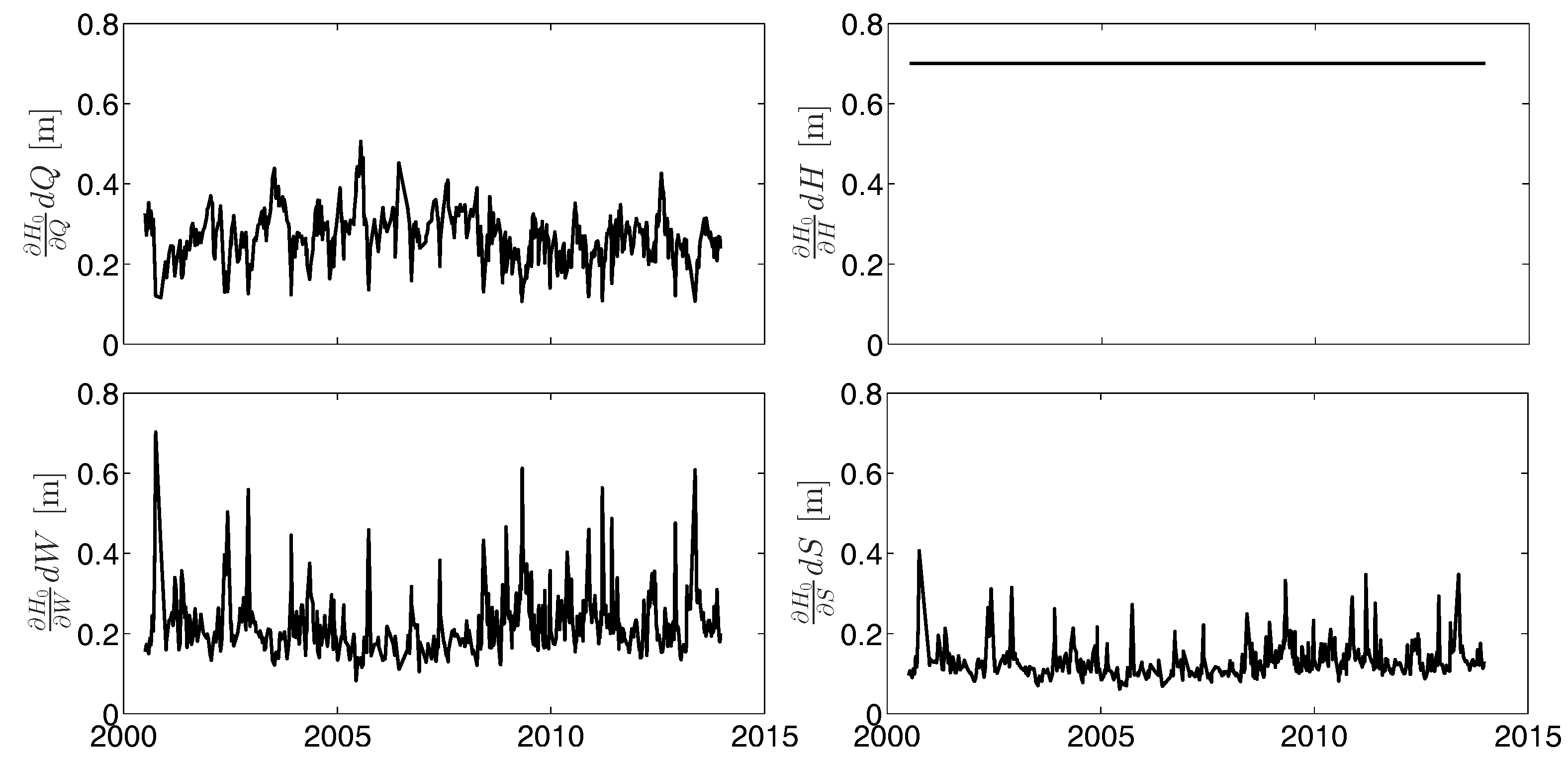
The sensitivities H 0 / Q , H 0 / W and H 0 / S depend on other parameters that are varying in time. In order to assess the error in H 0 due to the error of water level, width and discharge, here we assume a constant error of 0.7 m for water level time series from altimetry, which would lead to a constant error of 0.05 m/km for the slope of two consecutive reaches with a distance of 20 km (Equation (19)). For the effective river width, we use our time variable uncertainty estimates based on the method by [43]. For discharge, a multiplicative error of 10% is assumed. Figure 11 shows partial errors in H 0 due to the errors of other parameters in Reach 1. The contribution is about 0.2 m of the discharge’s precision on the precision of estimated H 0 . The average error in H 0 due to the errors of our width estimates is about 0.3 m. Since H 0 / S is time variable, a constant error in slope leads to a time variable error contribution with the average value of approximately 0.2 m for reach 1. This result shows that among all the parameters in Models (5) and (6), errors in height will contribute the most in the estimation of H 0 under the assumption that d H = 0.7 m .
Figure 12 shows the average of time series for the error contribution of different parameters over all 16 reaches. It is interesting to observe a large sensitivity of H 0 to slope for Reaches 15 and 16, at which we obtain a relatively large error. This means that for these reaches, the error in slope will be amplified with a larger error in the estimation of river depth. Moreover, the effects of errors in discharge and river width for the estimation of river depth are generally smaller than those for water level and slope.
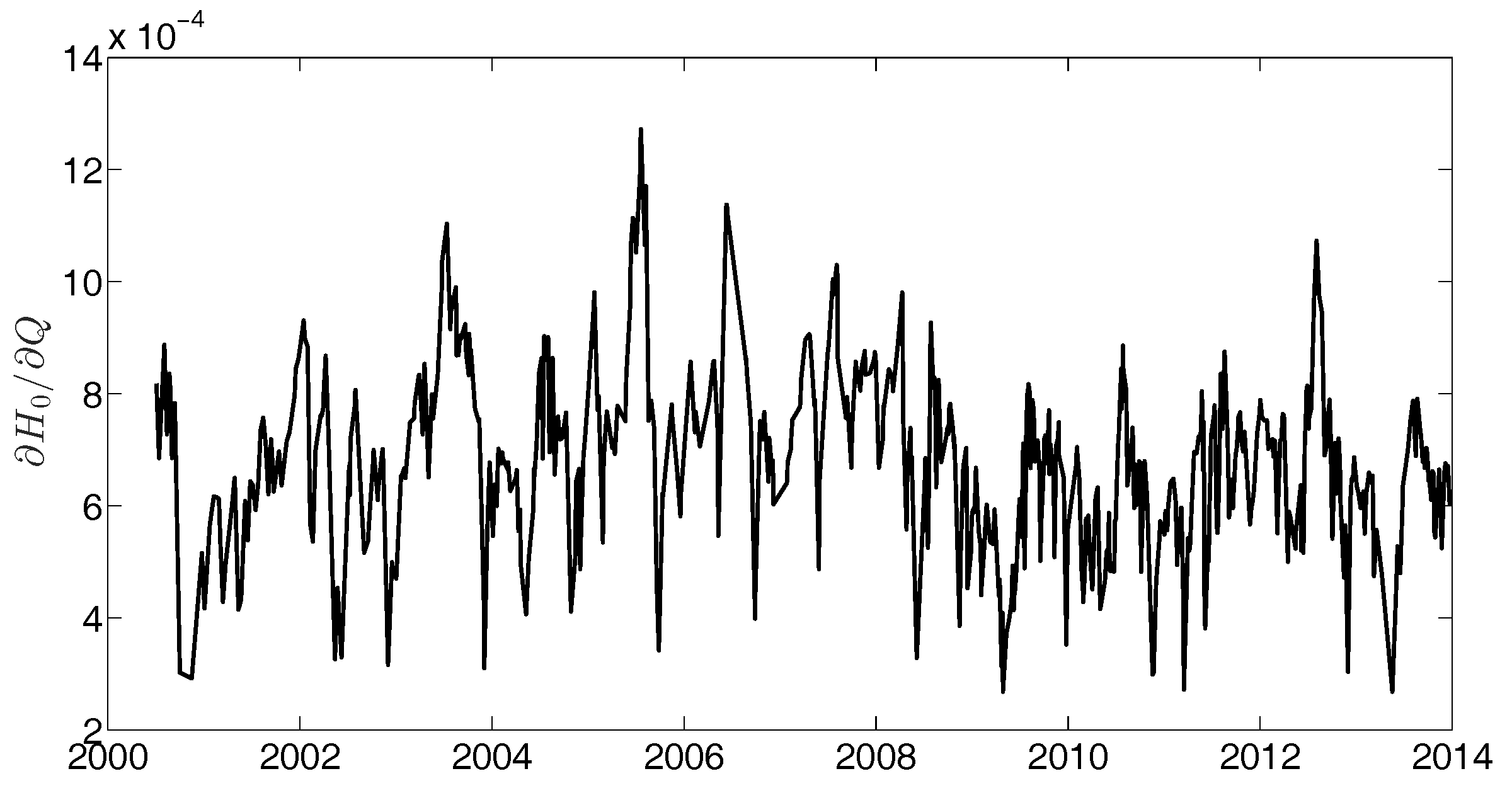
The direct formulation (21) is also beneficial for investigating why the estimation of H 0 is insensitive to the choice of discharge station. Figure 13 shows that H 0 / Q for Reach 1 varies between 3 × 10 4 and 12 × 10 4 with an average value of 6.8 × 10 4 . On the other hand, according to Table 3, average discharge at different stations is 933, 1075, 1313, 1378 and 1477 m 3 /s, respectively. This would mean that for the estimation of H 0 of Reach 1, a mischoice of Pontelagoscuro station with an average discharge of 1477 m 3 /s instead of Piacenza with an average discharge of 933 m 3 /s would lead to only 0.36 m error in H 0 ( 6.8 × 10 4 × ( 1477 933 ) = 0.36 ).

6. Perspective for the SWOT Mission

In the future, the SWOT mission will provide measurements of water surface elevation, river width and slope, through which discharge can be estimated for river widths down to 50–100 m, which allows us to obtain consistent and coherent information about the spatial distribution of river discharge. However, SWOT does not have the objective of and cannot be a replacement for in situ gauge networks [47]. SWOT will irregularly sample mid-latitude locations approximately three times per its 21-day cycle rather than nearly continuously, as in a gauge estimate. Although irregular sampling is appropriate to monitor the global water cycle, it is inadequate for many local-scale questions on rivers where SWOT may not fully observe temporal dynamics [11,47].
Moreover, SWOT will not observe full river networks. According to the study by [25] given the ability to observe rivers wider than 100 m, SWOT would observe more than 60% of the global sub-basins with an area of 50,000 km 2 . In terms of estimation of river depth, recent studies suggest that it may be possible to estimate river depth simultaneously from SWOT observations alone using multiple overpasses over several adjacent river reaches. However, studies are required to improve the understanding of the number of essential observations for a proper estimation of river depth [48].
The results in this study give a perspective of the SWOT mission and its scientific challenges in the following ways:
  • Satellite altimetry is put on an operational footing through the Sentinel 3 series of the European Copernicus program. At the same time, research satellites such as CryoSat-2, SARAL/AltiKa or Jason-3 remain in orbit and provide complementary space-time sampling. This constellation addresses many current limitations and opens a significant area of investigation into the operational use of altimetry missions for hydrological purposes. Developing methods to generate dense time series of water level using altimetry data, demonstrated in this study, raise the hope of using operational altimetry together with SWOT data in the future for a better monitoring of temporal dynamics in many rivers around the world.
  • Remote sensing techniques have been introduced as viable choices to monitor surface water variations [5]. Optical and SAR satellite imagery missions provide the opportunity to monitor surface water extent repeatedly at appropriate time intervals. Recent missions provide images with better spatial and temporal resolution. Different Landsat missions have been gathering images in various multispectral bands from the Earth since 1980. Recently, Landsat 8 with 30 m spatial resolution has provided monthly images of the Earth’s surface. Applications that demand a high temporal resolution preferably make use of the daily snapshots of MODIS imagery with 250-m resolution. Since 2015, Sentinel-2 has provided images with better resolution (10 m, 20 m, 60 m) and also a high revisit time (five days). On the other hand, SAR missions with images from ERS-1, ERS-2 and ENVISAT in C-band are the main sources for spatial water area monitoring in the tropical area, which is cloudy and rainy most of the year [12]. TerraSAR-X in X-band provides high resolution images with 1-, 2- and-3 meter pixel size every two days. From 2014 onwards, Sentinel-1A has provided continuous imagery (day, night and all weather) in C-band, expanding our understanding of surface water. Therefore, developing reliable algorithms to obtain reliable dynamic river masks, as developed by [38] and implemented in this study, gives the perspective of the SWOT mission that the results from different imagery sensors could be combined with the results from SWOT for a better monitoring of river masks in the future.
  • In terms of river depth estimation, our results in Figure 11, Figure 12 and Figure 13 highlight the weaker dependency of error in river depth estimation to the error of river width and river discharge. This means that a preliminary result of river width and a coarse river discharge would be enough to estimate river depth. This is especially important for discharge algorithms, which work based on Manning’s flow resistance equation, and the initial values of variables play an important role in the fast and precise estimation of discharge. Moreover, this result would mean that one could use a rough estimation of river discharge instead of in situ data and still receive acceptable results for river depth.

7. Summary and Conclusions

In this paper, we estimated the average river depth for 16 reaches along the Po River from SWOT-type observables water surface elevation, effective river width and slope using models by [9,36].
In order to obtain dense time series of water level from altimetry, we followed the method suggested by [39]. We connected all the virtual stations of several satellite altimeters along the Po River and produced water level time series at any location along the river. To this end, the selected altimetric measurements are stacked at the center of each reach by shifting the water level hydrographs of all virtual stations according to time lag between different virtual stations. The stacked measurements are then merged by normalizing the time series according to their statistical characteristics. After an outlier identification process, we rescaled the measurements back to their true water level values. For the densified time series at the 16 reaches, we obtained an effective temporal resolution of around three days from individual time series with originally a 10- or 35-day sampling interval. Time series of slope were obtained by differencing the time series of the water level at two consecutive reaches.
In order to derive effective width, we used MODIS images and extracted a dynamic river mask by employing the algorithm developed by [38]. This algorithm uses an MRF model regarding all sources of information available in images: spatial correlation between neighboring pixels and the long-term temporal behavior of the river. We then extracted the river mask in each image by maximizing a posteriori estimation in Markov random fields through minimizing the energy using the graph cuts technique. Although the graph cuts technique is preferred because of its ability to find a globally-optimal solution in polynomial time, it cannot provide any uncertainty measurement associated with the determined river mask. We have used the method by [43] to estimate uncertainty in the graph cuts solutions by measuring the max-marginal probability for each pixel. Following this, we generated a reliable river area time series together with its uncertainty.
With the help of the effective river width from satellite imagery, as well as water level and slope from satellite altimetry, we estimated river depth by implementing a Gauss–Helmert adjustment scheme on two models by [32,36]. Unlike variables observed from the space, discharge data are not available for each reach individually. We use discharge data at five in situ gauges along the river. An interesting result of this work is that the estimated H 0 for each reach only weakly depends on the choice of discharge data, since we obtained similar values for H 0 with a discrepancy of only ∼2% with the discharge data of different gauges. This result was explained by the low partials H 0 / Q , making the obtained H 0 less sensitive to the choice of discharge gauge.
We validated our results against surveyed cross-section information along the Po River. Validation shows general good agreement in the range of ∼10% relative RMSE. However, we faced some problematic reaches (4, 7, 8, 12, 15 and 16) for which the estimated H 0 is relatively large. We inconclusively discussed possible sources for such error by analyzing the quality of water level and effective river width time series. We have demonstrated that the water level time series generally correlate well (>0.6) with discharge data, and no specific pattern at the problematic reaches has been found. On the other hand, the correlation coefficients of effective river width with discharge data show generally small values especially at Reaches 1, 4 and 6. However, again, the reaches with a large error for the estimated H 0 do not show a distinctly lower correlation in comparison to other reaches.
The sensitivity analysis in this study especially demonstrates that the the estimated river depth is less influenced by the error of river width and river discharge, while it is strongly influenced by error in water level and slope. These results give a perspective of the SWOT mission, where the estimation of river depth would be possible using coarse estimates of river width and discharge and improved water level and slope time series. Moreover, this result would mean that one could use a rough estimation of river discharge instead of in situ data and still receive acceptable river depth. On the other hand, given the abundance of existing and future altimetry and imagery missions, developing methods to generate dense time series of water level using altimetry data and reliable river width from satellite imagery raises the hope of using operational altimetry and imagery including the Sentinel-series together with SWOT data in the future for a better monitoring of temporal dynamics in many rivers around the world.

Acknowledgments

The authors are grateful to the National Aeronautics and Space Administration (NASA) for providing the MODIS images at https://ladsweb.nascom.nasa.gov and the European Space Agency for providing the ENVISAT data at https://earth.esa.int/web/guest/data-access. Thanks are also due to AVISO for providing SARAL/AltiKa data through ftp://avisoftp.cnes.fr/AVISO/pub/saral/gdr_t/ and the Jason 2 hydrology product at ftp://ftpsedr.cls.fr/pub/oceano/pistach/J2/IGDR/hydro/. The authors would like to thank Angelica Tarpanelli for sharing the data of surveyed cross-sections along the Po River and the Agenzia Interregionale Fiume Po for providing the in situ data for the Po River, http://www.agenziainterregionalepo.it.

Author Contributions

Mohammad J. Tourian developed the method, conducted the data analysis and wrote the majority of the paper. Omid Elmi generated effective river width time series from satellite imagery and helped with analyzing the results and writing the manuscript. Abolfazl Mohammadnejad helped with analyzing results and writing the manuscript and also helped with the implementation of the Gauss-Helmert adjustment. Nico Sneeuw supervised the research, helped with the discussion of the method and contributed to manuscript writing.

Conflicts of Interest

The authors declare no conflict of interest.

Appendix A. Comparison of Water Level and Effective River Width with Discharge
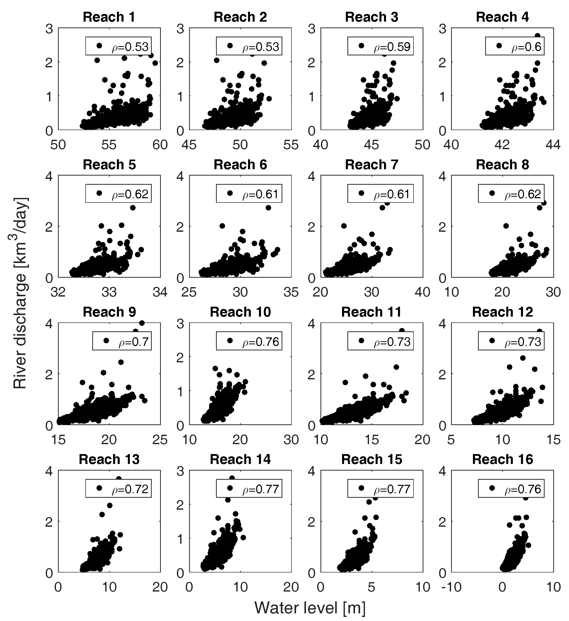
Figure A1 shows scatter plots of discharge at nearby gauging stations against water level time series for 16 reaches along the Po River. The water level time series show a generally good correlation (>0.6) with discharge data. Figure A2 shows the scatter plots for the effective river width time series for the 16 reaches. The correlation coefficients of effective river width with discharge data for all reaches are generally small especially at Reaches 1, 4 and 6. Since the Po River width is generally narrow for the MODIS pixels with 250 m resolution, such low correlation coefficients for the obtained river width are expected. Moreover, the river passes through many urban regions with managed channels, making the river width and discharge less correlated.
Figure A1. Comparison of water level time series and discharge at nearby gauging stations for 16 reaches along the Po River.
Water 09 00753 g014
Figure A2. Comparison of effective river width and discharge at close-by gauging stations for 16 reaches along the Po River.
Water 09 00753 g015
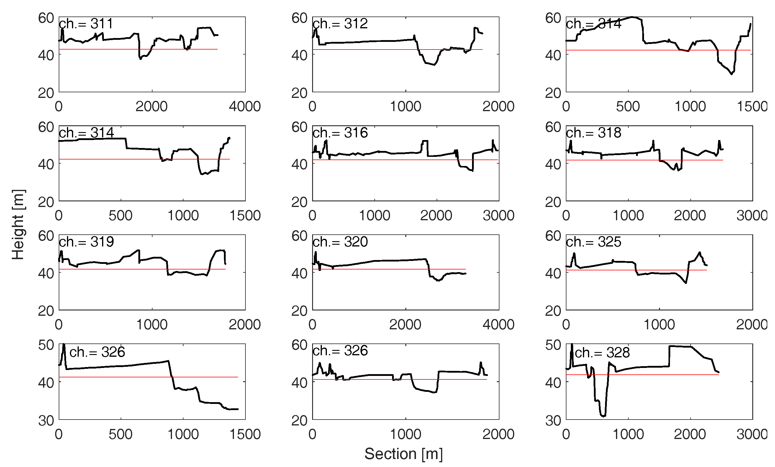
Figure A3 shows the surveyed sections along Reach 4 with the average water level at each section obtained from satellite altimetry. The section at Chainage 312, for instance, would lead to a non-homogeneous dependency between river width and discharge and would consequently lead to an inaccurate estimation of H 0 using the selected models. However, since we consider the averaged parameters of reaches, the effect of an individual problematic section on the final results should be negligible.
Figure A3. Sections along Reach 4. The red straight line represents the average water level obtained from altimetry.
Water 09 00753 g016

References

  1. Dingman, S.L.; Bjerklie, D.M. Estimation of River Discharge. In Encyclopedia of Hydrological Sciences; John Wiley & Sons, Ltd.: Hoboken, NJ, USA, 2006. [Google Scholar]
  2. Lorenz, C.; Devaraju, B.; Tourian, M.J.; Riegger, J.; Kunstmann, H.; Sneeuw, N. Large-scale runoff from landmasses: A global assessment of the closure of the hydrological and atmospheric water balances. J. Hydrometeorol. 2014, 15, 2111–2139. [Google Scholar] [CrossRef]
  3. Fekete, B.M.; Vörösmarty, C.J. The current status of global river discharge monitoring and potential new technologies complementing traditional discharge measurements. In Predictions in Ungauged Basins: PUB Kick-Off, Proceedings of the PUB Kick-Off Meeting, Brasilia, Brazil, 20–22 November 2002; IAHS Publication: Wallingford, UK, 2007; Volume 309. [Google Scholar]
  4. Tourian, M.J.; Sneeuw, N.; Bárdossy, A. A quantile function approach to discharge estimation from satellite altimetry (ENVISAT). Water Resour. Res. 2013, 49, 1–13. [Google Scholar] [CrossRef]
  5. Alsdorf, D.; Rodriguez, E.; Lettenmaier, D.P. Measuring surface water from space. Rev. Geophys. 2007, 45. [Google Scholar] [CrossRef]
  6. Tarpanelli, A.; Barbetta, S.; Brocca, L.; Moramarco, T. River Discharge Estimation by Using Altimetry Data and Simplified Flood Routing Modeling. Remote Sens. 2013, 5, 4145–4162. [Google Scholar] [CrossRef]
  7. Durand, M.; Andreadis, K.M.; Alsdorf, D.E.; Lettenmaier, D.P.; Moller, D.; Wilson, M. Estimation of bathymetric depth and slope from data assimilation of swath altimetry into a hydrodynamic model. Geophys. Res. Lett. 2008, 35, L20401. [Google Scholar] [CrossRef]
  8. Pavelsky, T.M.; Smith, L.C. RivWidth: A software tool for the calculation of river widths from remotely sensed imagery. Geosci. Remote Sens. Lett. IEEE 2008, 5, 70–73. [Google Scholar] [CrossRef]
  9. Bjerklie, D.M.; Dingman, S.L.; Vörösmarty, C.J.; Bolster, C.H.; Congalton, R.G. Evaluating the potential for measuring river discharge from space. J. Hydrol. 2003, 278, 17–38. [Google Scholar] [CrossRef]
  10. Elmi, O.; Tourian, M.J.; Sneeuw, N. River discharge estimation using channel width from satellite imagery. In Proceedings of the 2015 IEEE International Geoscience and Remote Sensing Symposium (IGARSS), Milan, Italy, 26–31 July 2015; pp. 727–730. [Google Scholar]
  11. Durand, M.; Gleason, C.J.; Garambois, P.A.; Bjerklie, D.; Smith, L.C.; Roux, H.; Rodriguez, E.; Bates, P.D.; Pavelsky, T.M.; Monnier, J.; et al. An intercomparison of remote sensing river discharge estimation algorithms from measurements of river height, width, and slope. Water Resour. Res. 2016, 52, 4527–4549. [Google Scholar] [CrossRef]
  12. Smith, L.C.; Isacks, B.L.; Bloom, A.L.; Murray, A.B. Estimation of discharge from three braided rivers using synthetic aperture radar satellite imagery: Potential application to ungaged basins. Water Resour. Res. 1996, 32, 2021–2034. [Google Scholar] [CrossRef]
  13. Kouraev, A.V.; Zakharova, E.A.; Samain, O.; Mognard, N.M.; Cazenave, A. Ob’ river discharge from TOPEX/Poseidon satellite altimetry (1992–2002). Remote Sens. Environ. 2004, 93, 238–245. [Google Scholar] [CrossRef]
  14. Andreadis, K.M.; Clark, E.A.; Lettenmaier, D.P.; Alsdorf, D.E. Prospects for river discharge and depth estimation through assimilation of swath-altimetry into a raster-based hydrodynamics model. Geophys. Res. Lett. 2007, 34, 481–496. [Google Scholar] [CrossRef]
  15. Gleason, C.J.; Smith, L.C. Toward global mapping of river discharge using satellite images and at-many-stations hydraulic geometry. Proc. Natl. Acad. Sci. USA 2014, 111, 4788–4791. [Google Scholar] [CrossRef] [PubMed]
  16. Durand, M.; Neal, J.; Rodriguez, E.; Andreadis, K.M.; Smith, L.C.; Yoon, Y. Estimating reach-averaged discharge for the River Severn from measurements of river water surface elevation and slope. J. Hydrol. 2014, 511, 92–104. [Google Scholar] [CrossRef]
  17. Garambois, P.A.; Monnier, J. Inference of effective river properties from remotely sensed observations of water surface. Adv. Water Resour. 2015, 79, 103–120. [Google Scholar] [CrossRef]
  18. Paiva, R.C.D.; Durand, M.T.; Hossain, F. Spatiotemporal interpolation of discharge across a river network by using synthetic SWOT satellite data. Water Resour. Res. 2015, 51, 430–449. [Google Scholar] [CrossRef]
  19. Lorenz, C.; Tourian, M.J.; Devaraju, B.; Sneeuw, N.; Kunstmann, H. Basin-scale runoff prediction: An Ensemble Kalman Filter framework based on global hydrometeorological data sets. Water Resour. Res. 2015, 51, 8450–8475. [Google Scholar] [CrossRef]
  20. Pan, M.; Wood, E.F. Inverse streamflow routing. Hydrol. Earth Syst. Sci. 2013, 17, 4577–4588. [Google Scholar] [CrossRef]
  21. Tourian, M.J.; Schwatke, C.; Sneeuw, N. River discharge estimation at daily resolution from satellite altimetry over an entire river basin. J. Hydrol. 2017, 546, 230–247. [Google Scholar] [CrossRef]
  22. Neal, J.; Schumann, G.; Bates, P.; Buytaert, W.; Matgen, P.; Pappenberger, F. A data assimilation approach to discharge estimation from space. Hydrol. Process. 2009, 23, 3641–3649. [Google Scholar] [CrossRef]
  23. Yoon, Y.; Durand, M.; Merry, C.J.; Clark, E.A.; Andreadis, K.M.; Alsdorf, D.E. Estimating river bathymetry from data assimilation of synthetic {SWOT} measurements. J. Hydrol. 2012, 464–465, 363–375. [Google Scholar] [CrossRef]
  24. Paiva, R.C.D.; Collischonn, W.; Bonnet, M.P.; de Gonçalves, L.G.G.; Calmant, S.; Getirana, A.; Santos da Silva, J. Assimilating in situ and radar altimetry data into a large-scale hydrologic-hydrodynamic model for streamflow forecast in the Amazon. Hydrol. Earth Syst. Sci. 2013, 17, 2929–2946. [Google Scholar] [CrossRef] [Green Version]
  25. Pavelsky, T.M.; Durand, M.T.; Andreadis, K.M.; Beighley, R.E.; Paiva, R.C.; Allen, G.H.; Miller, Z.F. Assessing the potential global extent of SWOT river discharge observations. J. Hydrol. 2014, 519 Pt B, 1516–1525. [Google Scholar] [CrossRef]
  26. Mersel, M.K.; Smith, L.C.; Andreadis, K.M.; Durand, M.T. Estimation of river depth from remotely sensed hydraulic relationships. Water Resour. Res. 2013, 49, 3165–3179. [Google Scholar] [CrossRef]
  27. Legleiter, C.J.; Roberts, D.A.; Marcus, W.A.; Fonstad, M.A. Passive optical remote sensing of river channel morphology and in-stream habitat: Physical basis and feasibility. Remote Sens. Environ. 2004, 93, 493–510. [Google Scholar] [CrossRef]
  28. Legleiter, C.J.; Roberts, D.A.; Lawrence, R.L. Spectrally based remote sensing of river bathymetry. Earth Surf. Proc. Landf. 2009, 34, 1039–1059. [Google Scholar] [CrossRef]
  29. Legleiter, C.J.; Roberts, D.A. A forward image model for passive optical remote sensing of river bathymetry. Remote Sens. Environ. 2009, 113, 1025–1045. [Google Scholar] [CrossRef]
  30. Fonstad, M.A.; Marcus, W.A. Remote sensing of stream depths with hydraulically assisted bathymetry (HAB) models. Geomorphology 2005, 72, 320–339. [Google Scholar] [CrossRef]
  31. Leon, J.; Calmant, S.; Seyler, F.; Bonnet, M.P.; Cauhop, M.; Frappart, F.; Filizola, N.; Fraizy, P. Rating curves and estimation of average water depth at the upper Negro River based on satellite altimeter data and modeled discharges. J. Hydrol. 2006, 328, 481–496. [Google Scholar] [CrossRef] [Green Version]
  32. Bjerklie, D.M. Estimating the bankfull velocity and discharge for rivers using remotely-sensed river morphology information. J. Hydrol. 2007, 341, 144–155. [Google Scholar] [CrossRef]
  33. Biancamaria, S.; Durand, M.; Andreadis, K.; Bates, P.; Boone, A.; Mognard, N.; Rodríguez, E.; Alsdorf, D.; Lettenmaier, D.; Clark, E. Assimilation of virtual wide swath altimetry to improve Arctic river modeling. Remote Sens. Environ. 2011, 115, 373–381. [Google Scholar] [CrossRef] [Green Version]
  34. Durand, M.; Rodriguez, E.; Alsdorf, D.E.; Trigg, M. Estimating river depth from remote sensing swath interferometry measurements of river height, slope, and width. IEEE J. Sel. Top. Appl. Earth Obs. Remote Sens. 2010, 3, 20–31. [Google Scholar] [CrossRef]
  35. Gejadze, I.; Malaterre, P.O. Discharge estimation under uncertainty using variational methods with application to the full Saint-Venant hydraulic network model. Int. J. Numer. Methods Fluids 2017, 83, 405–430. [Google Scholar] [CrossRef]
  36. Dingman, S.L.; Sharma, K.P. Statistical development and validation of discharge equations for natural channels. J. Hydrol. 1997, 199, 13–35. [Google Scholar] [CrossRef]
  37. Raggi, M.; Ronchi, D.; Sardonini, L. Po Basin Case Study Status Report; Deliverable D32; University of Bologna: Bologna, Italy, 2007. [Google Scholar]
  38. Elmi, O.; Tourian, M.J.; Sneeuw, N. Dynamic River Masks from Multi-Temporal Satellite Imagery: An Automatic Algorithm Using Graph Cuts Optimization. Remote Sens. 2016, 8, 1005. [Google Scholar] [CrossRef]
  39. Tourian, M.J.; Tarpanelli, A.; Elmi, O.; Qin, T.; Brocca, L.; Moramarco, T.; Sneeuw, N. Spatiotemporal densification of river water level time series by multimission satellite altimetry. Water Resour. Res. 2016, 52, 1140–1159. [Google Scholar] [CrossRef]
  40. Moramarco, T.; Singh, V.P. Simple Method for Relating Local Stage and Remote Discharge. J. Hydrol. Eng. 2001, 6, 78–81. [Google Scholar] [CrossRef]
  41. Ponce, V.M. Engineering Hydrology: Principles and Practices; Prentice Hall: Upper Saddle River, NJ, USA, 1989. [Google Scholar]
  42. Baarda, W. A Testing Procedure for Use in Geodetic Networks; Netherlands Geodetic Commission: Delft, The Netherlands, 1968; Volume 2. [Google Scholar]
  43. Kohli, P.; Torr, P. Measuring Uncertainty in Graph Cut Solutions efficiently Computing Min-marginal Energies Using Dynamic Graph Cuts. Comput. Vis. ECCV 2006, 1, 30–43. [Google Scholar]
  44. Te Chow, V. Open Channel Hydraulics; McGraw-Hill Book Company, Inc.: New York, NY, USA, 1959. [Google Scholar]
  45. Helmert, F.R. Die Ausgleichungsrechnung nach der Methode der Kleinsten Quadrate: Mit Anwendungen auf die Geodäsie und die Theorie der Messinstrumente; BG Teubner: Leipzig, Germany, 1872; Volume 1. [Google Scholar]
  46. Roese-Koerner, L.R. Convex Optimization for Inequality Constrained Adjustment Problems. Ph.D. Thesis, Universitäts-und Landesbibliothek Bonn, Bonn, Germany, 2015. [Google Scholar]
  47. Biancamaria, S.; Lettenmaier, D.; Pavelsky, T. The SWOT Mission and Its Capabilities for Land Hydrology. Surv. Geophys. 2016, 37, 307–337. [Google Scholar] [CrossRef]
  48. Pavelsky, T. Recent Progress in Development of SWOT river Discharge Algorithms. In Proceedings of the 2012 SWOT Discharge Algorithms Workshop, Chapel Hill, NC, USA, 18–20 June 2012; pp. 18–20. [Google Scholar]
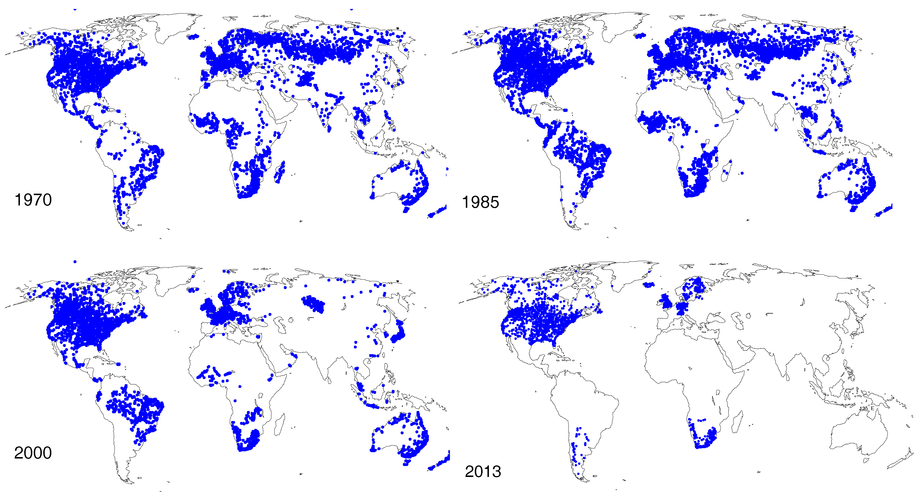
Figure 1. Available stations (updated in March 2017) with discharge data according to the Global Runoff Data Centre (GRDC) database (http://www.bafg.de/GRDC) for different years from 1970–2013.
Water 09 00753 g001
Figure 2. A schematic representation of a river with observable parameters (black) and unobservable ones (red, orange) from space. H 0 is the average riverbed’s height that does not correspond to the height of the deepest location in the channel section.
Water 09 00753 g002
Figure 3. The Po River flowing eastward in Italy. The red triangles indicate the location of virtual stations and the white ones the location of gauging stations from west to east: Piacenza, Cremona, Borgoforte, Sermide and Pontelagoscuro.
Water 09 00753 g003
Figure 4. (Top panel) Water level time series from satellite altimetry and effective river width from satellite imagery for Reach 12. (Bottom panel) Scatter plot of river discharge against water level (correlation coefficient = 0.73) and effective river width (correlation coefficient = 0.52).
Water 09 00753 g004
Figure 5. (Top panel) A MODIS image of the Po river with the selected river reaches. (Bottom panel) River mask extracted applying the proposed method by [38]. Date: 28 July 2000.
Water 09 00753 g005
Figure 6. Estimated river bed profile along the Po River for 16 defined reaches. VS refers to virtual station.
Water 09 00753 g006
Figure 7. Scatter plot of estimated H 0 using discharge data of different gauging stations along the Po River.
Water 09 00753 g007
Figure 8. Estimated river bed height by considering 20%, 40%, 60%, 80% and 100% of data in the time series of water level, width and discharge along the Po River for 16 defined reaches.
Water 09 00753 g008
Figure 9. Estimated residual for observations of discharge e Q ^ , water level e H ^ and effective river width e W ^ for the first reach along the Po River.
Water 09 00753 g009
Figure 10. Bar plot of difference between estimated riverbed’s height H 0 ^ and those from in situ using discharge data of different gauging stations along the Po River.
Water 09 00753 g010
Figure 11. Time series of error in H 0 due to the error in Q, H, W and S for Model (1) over Reach 1.
Water 09 00753 g011
Figure 12. Average error in H 0 due to errors in discharge, water level, effective river width and slope over all 16 reaches.
Water 09 00753 g012
Figure 13. The time variable sensitivity of estimated H 0 to discharge observation H 0 / Q .
Water 09 00753 g013
Table 1. Selected reaches along the Po River.
Reach NumberStarting PointEnding PointReach Length
Lat.Lon.ChainageLat.Lon.Chainage
( ° )( ° )(km)( ° )( ° )(km)(km)
145.119.12250.0045.109.34270.0020.00
245.109.34270.0045.119.55290.0020.00
345.119.55290.0045.089.66310.0020.00
445.089.66310.0045.079.82329.3619.35
545.079.82329.3645.099.90341.1611.80
645.099.90341.1645.0310.07369.3628.20
745.0310.07369.3645.0010.28389.3419.98
845.0010.28389.3444.9410.46409.3720.02
944.9410.46409.3744.9610.66429.3720.00
1044.9610.66429.3745.0410.79449.3620.00
1145.0410.79449.3645.0711.00469.3319.97
1245.0711.00469.3345.0611.21489.3620.03
1345.0611.21489.3644.9711.39509.3620.00
1444.9711.39509.3644.9211.57529.3419.98
1544.9211.57529.3444.9611.75549.3620.02
1644.9611.75549.3644.9811.98569.3519.99
Table 2. Summary of the datasets used in this study. AIPO, Agenzia Interregionale Fiume Po.
VariableDatasetResolutionTime PeriodSource
SpatialTemporal
Effective river width WMODIS250 m8 d2000–2014[38]
Variable Surface water level H and slope S Multi mission altimetry 3 d2000–2014[39]
TOPEX/Poseidon10 d1992–2002
ENVISAT35 d2002–2010
TOPEX/Poseidon XT10 d2002–2005
ENVISAT XT30 d2010–2012
CryoSat-2369 d2012–2014
Jason-210 d2008–2016
River discharge Qin situ1 d1995–2013AIPO
Channel sectionssurveyedevery 250 mAIPO
Table 3. The location and height of available in situ data along the Po River. The height refers to the mean water level derived from daily time series.
NameLat.Lon.ElevationAverage WidthAverage Flow VelocityAverage Discharge
( ° )( ° )(m)(km)(m/s)(m 3 /s)
Piacenza45.069.7042.371060.61933
Cremona45.139.9929.031570.821075
Borgoforte45.0510.7514.051640.841313
Sermide45.0211.299.503290.441378
Pontelagoscuro44.8911.613.481753.011477
Table 4. Estimated river bed height H 0 using the two selected models, for which discharge data of the nearest gauge are used.
Reach H 0 ins (m)Model by Bjerklie et al. [9]Model by Dingman and Sharma [36]
a ^ H 0 ^ (m) H 0 ^ H 0 ins (m) a ^ H 0 ^ (m) H 0 ^ H 0 ins (m)
150.270.6950.37 ± 0.150.100.3950.66 ± 0.140.39
245.620.6044.72 ± 0.150.890.3044.96 ± 0.140.66
340.091.3641.47 ± 0.101.380.6741.69 ± 0.091.59
435.912.0640.73 ± 0.034.830.8840.85 ± 0.034.94
532.2029.2032.07 ± 0.010.1211.9532.13 ± 0.010.07
624.600.8024.91 ± 0.090.310.4025.16 ± 0.080.57
720.630.2216.06 ± 0.314.560.1316.53 ± 0.314.10
817.180.2713.06 ± 0.264.120.1613.58 ± 0.263.60
912.920.7412.07 ± 0.140.850.4212.48 ± 0.130.44
1011.540.509.37 ± 0.162.170.279.77 ± 0.161.77
117.380.537.04 ± 0.160.340.297.48 ± 0.160.10
122.701.405.64 ± 0.072.940.735.91 ± 0.073.21
132.081.253.00 ± 0.100.920.663.31 ± 0.091.23
14−0.260.58−1.49 ± 0.201.230.34−0.87 ± 0.190.61
15−3.004.831.07 ± 0.044.072.281.23 ± 0.044.24
16−6.294.97−1.32 ± 0.084.972.64−1.07 ± 0.075.22