Assessing Agricultural Drought in the Anthropocene: A Modified Palmer Drought Severity Index

1. Introduction

Drought is one of the most common hazards that can occur in anywhere of the world and has a wide range of impacts and consequences. The frequency and severity of droughts have increased over the past decade. From 2001 to 2002, Canada suffered the most severe drought of the last 100 years, which resulted in C$5.8 billion losses. The Central Plains in the United States suffered a severe drought during 2012 and 2013 which caused losses of $12 billion [1]. Drought is usually defined as an abnormal water deficit that lasts over several weeks to months due to no or little accumulated rainfall [2]. Meteorologists, hydrologists and agriculturists have made their own definitions of drought from their different fields, and classified it into meteorological drought, hydrological drought, and agricultural drought accordingly. Therefore, numerous drought indices have been established and applied to drought research over the decades, with favorable practical applications, such as the: Palmer drought severity index (PDSI) [3]; the crop moisture index [4]; the surface water supply index [5]; the crop-specific drought index [6]; the vegetation condition index [7]; the standardized precipitation index [8]; the soil moisture deficit index [9]; and the standardized soil moisture index [10].

However, traditional definitions have viewed drought as a natural phenomenon, and previous approaches to drought research have operated in relative isolation without considering the complex interactions between natural and anthropogenic processes. Human activities on water resources development and utilization notably alter hydrological processes such as evapotranspiration, runoff and infiltration and the amount of water stored in the soil, rivers, groundwater, lakes and reservoirs [11]. When there is less water than normal in any system, the system is perceived to be in drought, no matter whether this is due to meteorological or anthropogenic causes [12]. Consequently, the traditional unidirectional drought indices result in poor evaluation and monitoring, especially in areas of high human intervention [11].

Drought in areas of high human intevention, such as Australia, Central Asia, California in the USA, China and India, should not be seen as purely natural, but as a complex interdisciplinary phenomenon [11]. Drought is a coupling effect of natural and human drivers [13,14,15,16], and anthropogenic responses to the natural environment can modify the occurrence, development and severity of drought [17,18]. Also, agricultural drought is associated with previous meteorological conditions, existing soil moisture, irrigation, crop varieties and different characteristics at growth stages and so on [19]. Humans can take various measures to respond to agricultural drought, such as irrigation, water transfer, implementing water-saving counter-measures, strengthening water rights management, and adjusting the cropping structure. Irrigation, an important form of human agricultural activity, is vital to production for its role in not only pursuing higher yields per unit area, but also preventing drought on farmland. Irrigated land represents only 20% of global cropland but generates 40% of the crops [20]. There are many important agricultural regions dominated by irrigated agriculture, such as Bangladesh, China, Central Asia, Pakistan and India [21]. In India, 43% of the arable land is irrigated [22], and in China, irrigation is used on 40% of the arable area [23]. As a typical human intervention, irrigation is no longer a passive action for resisting drought in some countries, but a conventional agricultural activity. For instance, in China, according to the established irrigation schedule, the fields are irrigated quantitatively within specific days, whether drought occurs or not. This irrigation treatment does not guarantee that no drought occurs later, but keeps the farmland soil moisture and ensures grain production.

Developed and larger scale irrigation systems have greatly guaranteed grain production in those countries and areas that are dependent on irrigation to support agricultural development [24]. Even in some dry years with less precipitation and high temperatures, people can still have a good harvest. Therefore, it is likely that an important question may arise when assessing agricultural drought: owing to the irrigation water supplement, farmland soil moisture is higher than that without irrigation [25]. Thus, drought may be delayed, weakened, or it can even end rapidly. That is, the actual severity of droughts may be distorted by traditional approaches due to human intervention in some cases. This inconsistency between actual and monitoring results leads to a new scientific problem that needs to be explained and investigated. Natural and anthropogenic drivers should be integrated into drought definitions and analytical approaches [25]. To this end, Van Loon et al. [11,25] redefined the concept of drought by considering the influence of human activity on the emergence and development of drought. Van Loon et al. [25] argued that drought in the Anthropocene is a temporary lack of water compared to normal conditions for a specific system caused by multiple interactions between natural hydro-climatological processes and human influence. Human modifications to drought enhance or alleviate its severity, and long-term human feedback to the environment or drought alters the assessment baseline (the normal water conditions for specific systems in a region) that determines the occurrence and severity of droughts.

Accessible tools that are simple to construct are indispensable for assessing human-influenced drought, but currently few of them have been developed. To this end, a simple and effective drought index considering both natural and human drivers is urgently needed to assess the actual severity of agricultural droughts in areas of high human intervention. The PDSI is a well-known drought index that has enjoyed an excellent reputation in many countries [26,27,28,29,30,31]. The PDSI is also widely used for agro-climatological analysis [3,32], and it has been demonstrated to be a useful agricultural drought-evaluation tool in multiple studies [33,34,35,36,37]. It has been found that PDSI values are significantly correlated with the measured soil moisture content, especially in the warm crop-growing season [38,39]. According to the definition of drought in the Anthropocene, this study presents an agricultural drought index for assessing human-modified agricultural drought in irrigated farming regions based on the Palmer drought severity index by considering irrigation activity. The Haihe River Basin in northeast China was selected, as an area typifying high human intervention characteristics and have large areas of irrigated agriculture. The water balance model in the PDSI was modified by taking irrigation into account. Moreover, the proposed drought index takes into consideration irrigation quotas by auto-irrigation settings during specific growth stages of specific crops (wheat–corn). The applicability of the new index was validated by analyzing the soil moisture, the frequency of the weekly index values, and the spatial-temporal distribution of agricultural droughts.

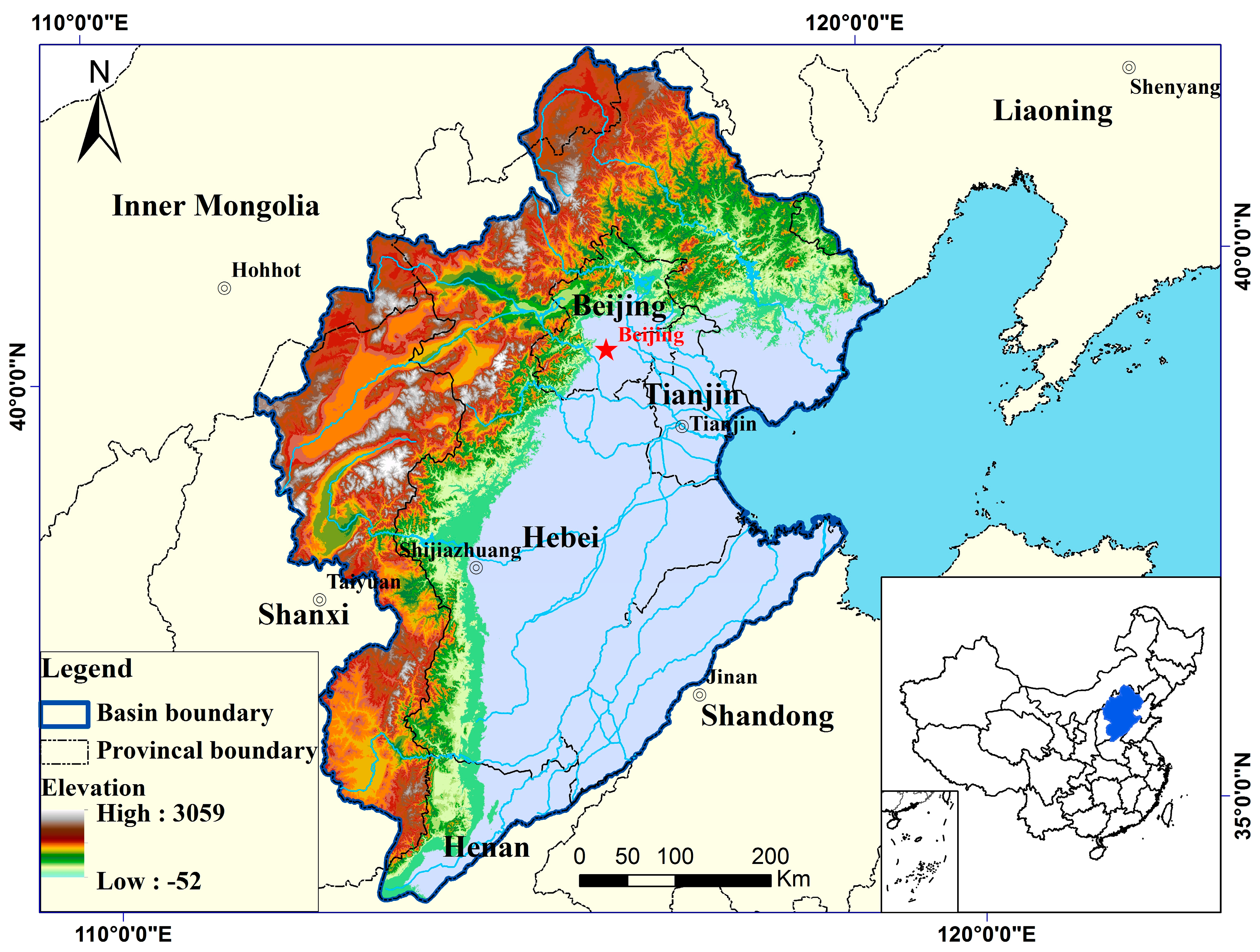
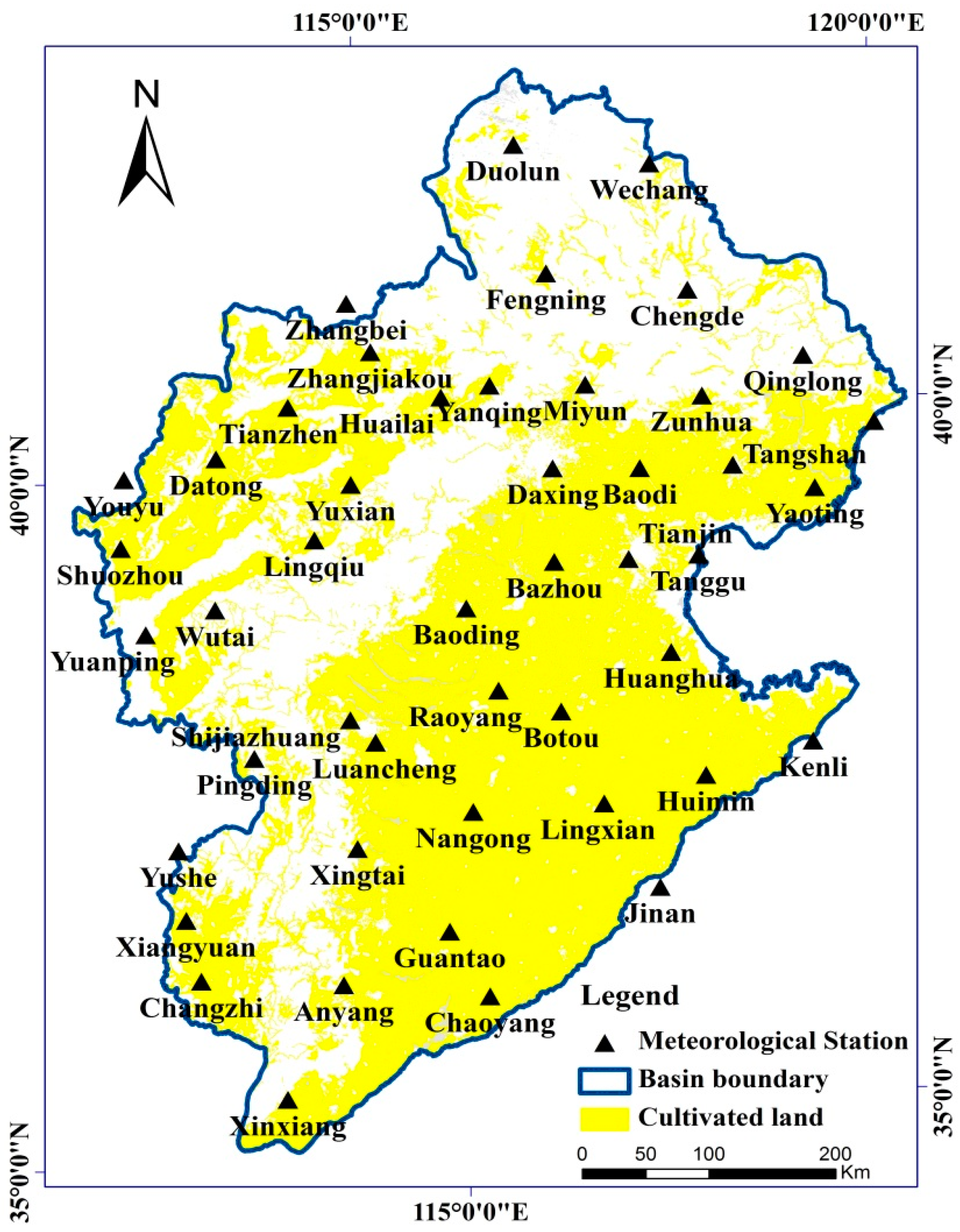
2. Description of the Study Area

The Haihe River Basin is located in northeast China between 112–120° E and 35–45° N (Figure 1). It is the eighth largest river basin in China, with a drainage area of 320,041 km² [22], accounting for approximately 3.4% of the total national area. The Haihe River Basin faces the Bohai Sea to the east and the Loess Plateau to the west, and it adjoins the Yellow River in the south and the Yanshan Mountains in the north, according to the northwest Inner Mongolian Plateau. The mountains and plateaus in the north and west of the basin take up around 60% of the whole area, and have temperate grassland plants and warm temperate deciduous broad-leaved forest [40]. The eastern and southeastern areas mainly comprise the North China Plain, which has a long history of agricultural reclamation and is one of the major grain production areas in China. The double cropping system of winter wheat–summer maize is predominant in the plain area [41,42] and the single cropping system of spring maize is distributed mainly in northern parts of Hebei and Shanxi Provinces.

The study area is located in a transition region between humid and arid climates with four distinct seasons: hot, rainy summers and cold, dry winters. The average temperature varies from 4 °C to 14 °C and the annual precipitation varies from 371 mm to 771 mm [43]. The precipitation in summer is heavy, and about two-thirds of this falls during June and September. In spring, the precipitation is less than 100 mm, and accounts for merely 18% of the total annual precipitation, far less than the water requirement for growing winter wheat. Drought occurs frequently as a result of low precipitation, a rapid increase of temperature and large evapotranspiration, and it is the main threat to the production of winter wheat in this area. For this reason, irrigation is vital for promoting crop growth and improving yields. Currently, the irrigated area makes up more than 80% of the total cultivated land in the Haihe River Basin.

3. Data and Methodology

3.1. Data Sources

The daily time series of precipitation, relative humidity, average wind speed, sunshine hours and air temperature (minimum and maximum) from 47 meteorological stations between 1985 and 2012 were used in this study (Figure 2). The data was provided by the China Meteorological Science Data Sharing Service Network (http://data.cma.cn/). Soil data for the study area, including soil texture, saturated water content, field capacity, and wilting coefficient, was provided by the China Soil Science Database (http://www.soil.csdb.cn/). Irrigation data for the study area was from 1985 to 2012. The data adopted herein was obtained from the Haihe River Basin Water Resources Bulletin, and Statistical Yearbook of the five provinces (Beijing, Tianjin, Hebei, Henan, Shandong and Shanxi). The experimental data for soil water content within the top 1 m depth during 2007 and 2012, was provided by Luancheng Agro-Ecosystem Experimental Station, Chinese Academy of Sciences, Shijiazhuang, Hebei Province.

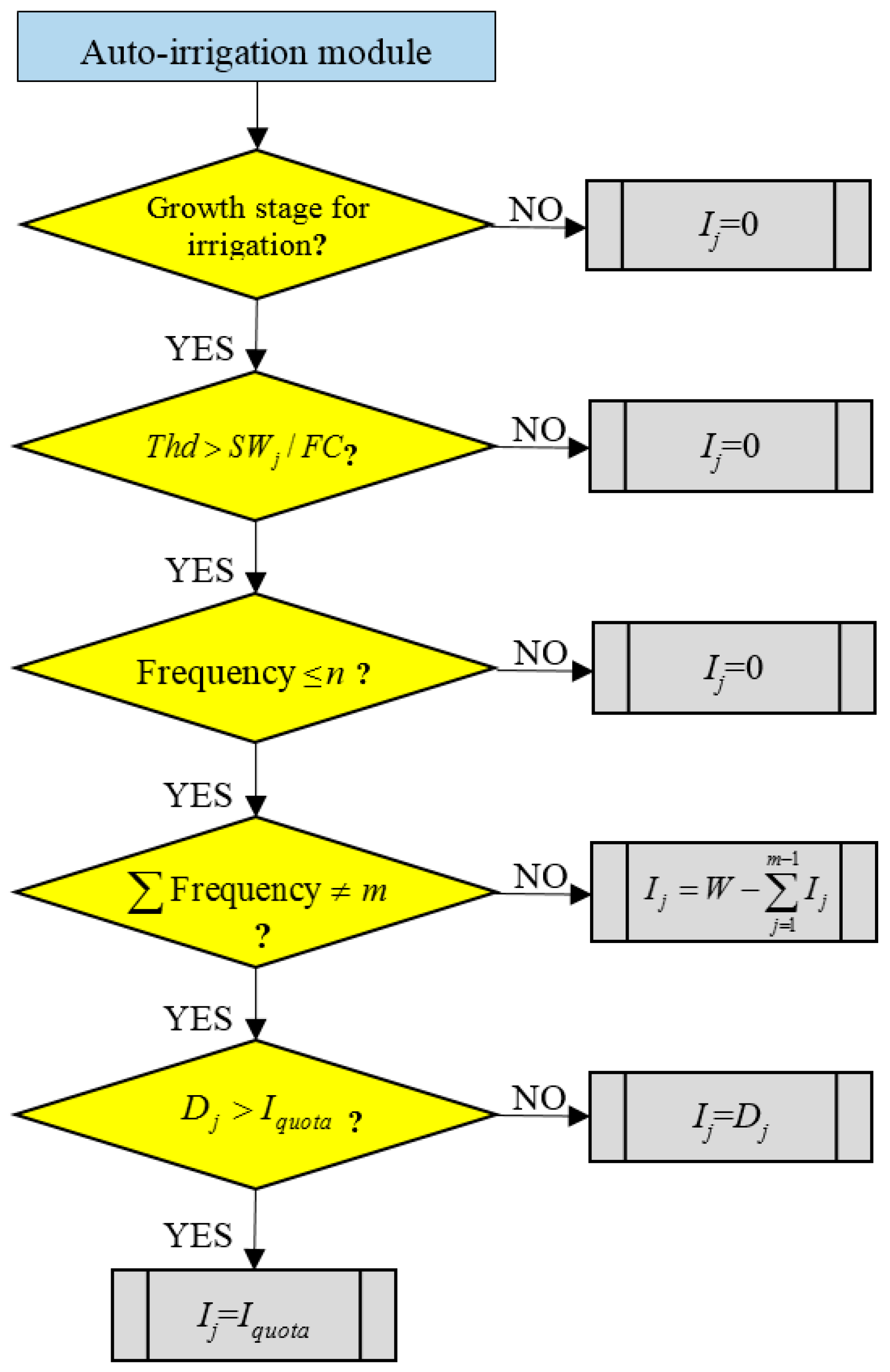
3.2. Methodology

The following explanation describes in detail how to calculate the new drought index considering irrigation processes (IrrPDSI), and it is a new method based on Palmer’s approach [3].

Palmer’s method begins with a water balance equation. In this work, one major human driver, irrigation, is taken into account, and the time step is shortened to one week in accordance with the characteristics of agricultural drought in order to accurately reflect the soil moisture change and increased sensitivity to short-term wet and dry changes. The modified water balance equation is expressed as follows.

$${\stackrel{⌢}{Q}}_i=E{\stackrel{⌢}{T}}_i+R{\stackrel{⌢}{O}}_i+{\stackrel{⌢}{R}}_i-{\stackrel{⌢}{L}}_i$$

(1)

where ${\stackrel{⌢}{Q}}_i$ is the CAFEC (climatically appropriate for existing conditions) water supply (the sum of the precipitation and irrigation) in week i; and $E{\stackrel{⌢}{T}}_i$, $R{\stackrel{⌢}{O}}_i$, ${\stackrel{⌢}{R}}_i$ and ${\stackrel{⌢}{L}}_i$ are the CAFEC quantities for evapotranspiration, runoff, recharge and loss in week i, respectively.

$E\stackrel{⌢}{T}$, $\stackrel{⌢}{R}$, $R\stackrel{⌢}{O}$ and $\stackrel{⌢}{L}$ are calculated with original formulas [1].

$$\begin{array}{l}E{\stackrel{⌢}{T}}_i=\overline{E{T}_i}/\overline{P{E}_i}\cdot P{E}_i{\stackrel{⌢}{R}}_i=\overline{R_i}/\overline{P{R}_i}\cdot P{R}_i\\ R{\stackrel{⌢}{O}}_i=\overline{R{O}_i}/\overline{PR{O}_i}\cdot PR{O}_i{\stackrel{⌢}{L}}_i=\overline{L_i}/\overline{P{L}_i}\cdot P{L}_i\end{array}$$

(2)

where PE_i, PL_i, PR_i, and PRO_i are the potential evapotranspiration, recharge, loss and runoff in week i, respectively; and ET_i, L_i, R_i, and RO_i are the actual evapotranspiration, recharge, loss and runoff in week i, respectively. The bar over a term indicates an average value.

PL, PR and PRO are also calculated with original methods.

$$\begin{array}{l}P{L}_{s,i}=Min\left(P{E}_i,S_{s,i}\right)\\ P{L}_{u,i}=\left(P{E}_i-P{L}_{s,i}\right)\cdot S_{u,i}/AWCP{L}_{u,i}\le S_{u,i}\\ P{L}_i=P{L}_{s,i}+P{L}_{u,i}\end{array}$$

(3)

$$P{R}_i=AWC-\left(S_{s,i}+S_{u,i}\right)$$

(4)

$$PR{O}_i=AWC-P{R}_i$$

(5)

where PL_s,i and PL_u,i are the potential water loss from the surface and underlying layers in week i (mm), respectively. PE_i is the potential evapotranspiration in week i (mm), which was calculated by the Penman–Monteith method; AWC is the combined available moisture capacity (mm); and S_s,i and S_u,i represent the initial available moisture stored in the surface and underlying layers in week i (mm), respectively.

A two-layer bucket-type model is applied to carry out the hydrological accounting in Palmer’s method. It is assumed that moisture supply was adequate when rainfall exceeded PE. The moisture loss is assumed to take place at the potential rate and as residual water entered the soil. If rainfall was less than PE and did not meet evapotranspiration, soil moisture was lost. Evapotranspiration is equal to the sum of the amount of precipitation and water loss. Now irrigation is considered, and moisture supply (Q) is equal to the sum of the precipitation and irrigation (Q = P + I). If Q exceeds PE, the actual evapotranspiration ET was equal to PE. Otherwise, ET was equal to the sum of precipitation and the water lost. Therefore,

$$E{T}_i=\{\begin{array}{l}P{E}_{i}P{E}_i\le P_i+I_i\\ P_i+L_{i}P{E}_i>P_i+I_i\end{array}$$

(6)

where PE_i and ET_i are the potential evapotranspiration and actual evapotranspiration in week i respectively (mm), I_i is the irrigation amount in week i (mm), P is the precipitation in week i (mm).

Similarly, if moisture supply Q was less than PE, and was not enough to maintain evapotranspiration, soil moisture was lost. It is assumed that moisture cannot be lost from the underlying layer until all of the available moisture has been removed from the surface layer and water loss from the underlying layer is affected by the initial soil moisture, PE, and AWC. Water loss L is equal to the sum of water loss from the surface and the underlying layer.

$$L_i=\{\begin{array}{l}0P_i+I_i\ge P{E}_i\\ L_{s,i}+L_{u,i}{P}_i+I_i<P{E}_i\end{array}$$

(7)

Water loss from the surface and the underlying layer

$$L_{s,i}=Min\left(P{E}_i-P_i-I_i,S_{s,i}\right)$$

(8)

$$L_{u,i}=\left(P{E}_i-P_i-I_i-L_{s,i}\right)\cdot S_{u,i}/AWC$$

(9)

where S_s,i and S_u,i represent the initial available moisture stored in the surface and underlying layers in week i respectively (mm); I_i is the irrigation amount in week i (mm); and the L_s,i and L_u,i represent the water loss from the surface and underlying layers in week i, respectively (mm).

It is assumed that no recharge occurs until the moisture supply Q exceeds PE. And recharge R is equal to the potential recharge PR if both layers reach field capacities, otherwise R is equal to Q minus PE. Therefore,

$$R_i=\{\begin{array}{ll}0\hfill & P_i+I_i\le P{E}_i\hfill \\ P_i+I_i-P{E}_i\hfill & 0<P_i+I_i-P{E}_i<P{R}_i\hfill \\ P{R}_i\hfill & P_i+I_i-P{E}_i\ge P{R}_i\hfill \end{array}$$

(10)

Runoff is assumed to occur only if both layers reach field capacity.

$$R{O}_i=P_i+I_i-E{T}_i-P{R}_i$$

(11)

where PR_i is the potential recharge in week i (mm), and RO_i is the runoff in week i (mm).

Unlike precipitation data that are routinely available via a network of meteorological stations, the data for irrigation timing and amount are virtually impossible to measure or record, and therefore national statistical databases may be a good source of information [25]. To this end, the data of the annual irrigation quantity per unit area from 1985 to 2012 was selected for this work, and was obtained from the Statistical Yearbook of the five provinces (Beijing, Tianjin, Hebei, Henan, Shandong and Shanxi). Irrigation is implicated when the soil water condition reaches the auto-irrigation threshold in every growth stage. The annual irrigation quantity is allocated to every irrigation implication in the growing season of the year, based on the soil water deficit and irrigation water quotas for each growth stage.

The auto-irrigation threshold is a ratio of soil moisture to field capacity. The threshold in each growth stage was set based on the crop growth requirement for soil moisture that varies in every growth stage. The auto-irrigation implication is applied only when the soil moisture content was lower than the threshold. In a specified growth stage for n weeks, the irrigation amount in week j (j = 1, 2,…, n) is represented as

$$I_j=\{\begin{array}{ll}0& Thd\le S{W}_j/FC\\ Min\left(D_j, I_{quota}\right)& Thd>S{W}_j/FC\end{array}$$

(12)

$${\displaystyle \sum _{j=1}^m{I}_j}=W$$

(13)

where j is the jth week during the specified growth stage; I_j is the irrigation amount in week j (mm); Thd represents the auto-irrigation threshold in the specified growth stage; SW_j is the initial soil moisture content in week j (mm); FC respects the field capacity (mm); D_j is the soil water deficit in week j (mm); I_quota is the irrigation quota in the specified growth stage (mm); m is the annual frequency of irrigation; and W is the annual irrigation quantity per unit area (mm). The irrigation amount varies in different periods of crop growth. In this study, the irrigation quota is based upon irrigation scheduling in the Haihe River Basin, as shown in

Table 1. The irrigation scheduling in the Haihe River Basin.

Region	Crop Type	Growth Stage for Irrigation	Irrigation		Auto-Irrigation Threshold d
			Frequency	Amount (mm)
Western Hebei, Beijing, Tianjing and south Shanxi a	Winter wheat	Sowing (1–10 Octobor)	1	58	0.6
		Tillering (20 November–10 December)	1	80	0.5
		Jointing (10 March–14 April)	1	65	0.55
		Heading (10–30 April)	1	68	0.55
		Filling (1–30 May)	2	75	0.55
				67	0.55
	Summer maize	Jointing (1–30 July)	1	64	0.55
		Filling (20 August–20 September)	1	64	0.6
Northern Shandong, northern Henan and eastern Hebei b	Winter wheat	Sowing (15–30 Octobor)	1	63	0.6
		Tillering (20 November–10 December)	1	70	0.5
		Jointing (10 March–14 April)	1	65	0.55
		Heading (10–30 April)	1	70	0.55
		Filling (1–30 May)	2	67	0.55
				65	0.55
	Summer maize	Jointing (1–20 July)	1	61	0.55
		Filling (1–30 August)	1	71	0.6
Northern Shanxi and northern Hebei c	Spring maize	Jointing (10 June–10 July)	1	75	0.55
		Tasseling (20–30 July)	1	75	0.6
		Filling (1–30 August)	1	75	0.6

Notes: ^a The data was provided by Luancheng Agro-Ecosystem Experimental Station, Chinese Academy of Sciences, Shijiazhuang, Hebei Province; ^b The data was obtained from Liu et al. [45]; ^c The data was obtained from Xiao et al. [46]; ^d The data was obtained from the SL 568-2012 [47].

.

The soil water deficit in week i is expressed as follows

$$D_i=\{\begin{array}{ll}0\hfill & AWC-\left(S_{s,i}+S_{u,i}\right)\le P_i\hfill \\ AWC-\left(S_{s,i}+S_{u,i}\right)-P_i\hfill & AWC-\left(S_{s,i}+S_{u,i}\right)>P_i\hfill \end{array}$$

(14)

where D_i is the soil water deficit in week i (mm); AWC is the combined available moisture capacity (mm); and S_s,i and S_u,i represent the initial available moisture stored in the surface and underlying layers in week i (mm), respectively.

The flow chart of the auto-irrigation procedure is presented in Figure 3. The main steps are described as follows:

Step 1: For week j in a specified growth stage, according to the irrigation scheduling, if week j is not in the growth stage for irrigation (such as the jointing stage shown in Table 1), no irrigation occurs (I_j = 0), otherwise, go to the next step.

Step 2: According to the Equation (15), if the ratio of soil moisture to field capacity for week j is higher than the auto-irrigation threshold in the specified growth stage (for example, for the jointing stage for spring maize showed in Table 1, Thd = 0.55), I_j = 0, otherwise, go to the next step.

Step 3: According to the irrigation scheduling, the times of irrigation allocated must not exceed the irrigation frequency n in the specified growth stage (for example, for the jointing stage for spring maize showed in Table 1, n = 1). If not, I_j = 0.

Step 4: If it is the last irrigation in this year (${\displaystyle \sum \mathrm{Frequency}}=m$), $I_j=W-{\displaystyle \sum _{j=1}^{m-1}{I}_j}$, otherwise, go to the next step.

Step 5: If the soil water deficit in week i (D_j) is higher than the irrigation quota in the specified growth stage (for example, for the jointing stage for spring maize showed in Table 1, I_quota = 75 mm), I_j = I_quota, otherwise, I_j = D_j.

The calculation of the moisture departure should be changed accordingly. The moisture departure d is the sum of rainfall and irrigation minus the climatically appropriate moisture supply.

$$\begin{array}{l}{d}_i=P_i+I_i-{\stackrel{⌢}{Q}}_i\\ =P_i+I_i-\left({\alpha }_i\cdot P{E}_i+{\gamma }_i\cdot PR{O}_i+{\beta }_i\cdot P{R}_i-{\delta }_i\cdot P{L}_i\right)\end{array}$$

(15)

The moisture departure d means different things at different times, as well as at different locations, and this prevented its applicability [32,44]. To correct for this, an empirically derived climate-weighting factor, K, was used to adjust the value of d. The result of multiplying the moisture departure, d, by K is called the Palmer-Z index [3], and it is defined as

$$Z_i=K_i\cdot d_i$$

(16)

where K is actually a refinement of $K\prime$, which is the general approximation for the climate characteristic of a location [32]. K is expressed as

$$K_i=\frac{610.35}{{\displaystyle {\sum }_{i=1}^N{\overline{D}}_i{K}_i^{\prime }}}{K}_i^{\prime }$$

(17)

where ${\overline{D}}_i$ is the average of the absolute values of d for week i, and N is the number of weeks. The annual sums of $\overline{D}{K}^{\prime }$ from 47 stations in the Haihe River Basin range from 296.4 to 850.2, and the value of 610.35 in Equation (17) is the average value of the 47 stations.

According to Palmer’s paper [3], the average annual weighting factor $\overline{K\prime }$ is related to the average annual moisture demand $\overline{PE}+\overline{R}+\overline{R}O$, the average annual moisture supply $\overline{Q}+\overline{L}$ and the average annual absolute moisture anomaly $\overline{D}$. Thus, an empirical relationship between 47 stations in the Haihe River Basin is derived (Figure 4), and the formulation was applied to each week in each of the stations to derive the weekly weighting factor $K\prime$, which is expressed as

$$K_i^{\prime }=1.42\ln \left(\frac{\overline{P{E}_i}+\overline{R_i}+\overline{R{O}_i}}{\overline{Q_i}+\overline{L_i}}/\overline{D_i}\right)+4.68$$

(18)

Here the bar over a term in Equation (20) indicates an average value and the weekly ET, L, R, RO and other parameters of 47 stations are computed based on Equations (1)–(15).

An empirical formula for determining drought severity is given by the equation

$$X_i=0.785X_{i-1}+Z_i/45.491$$

(19)

where X_i is the PDSI value for the ith week and X_i−1 is previous week’s PDSI value.

Equations (16)–(19) are the final expression of IrrPDSI in the Haihe River Basin. Palmer’s 11 categories shown in

Table 2. Classification of the Palmer drought severity index (PDSI) values.

PDSI Value	Class
≥4.00	Extreme wet
3.00 to 3.99	Severe wet
2.00 to 2.99	Moderate wet
1.00 to 1.99	Mild wet
0.50 to 0.99	Incipient wet
0.49 to −0.49	Normal
−0.50 to −0.99	Incipient drought
−1.00 to −1.99	Mild drought
−2.00 to −2.99	Moderate drought
−3.00 to −3.99	Severe drought
≤−4.00	Extreme drought

continue to be used.

Table 3. Comparison of the computational formulas of the two indices.

PDSI	IrrPDSI
$\begin{array}{l}L=\{\begin{array}{ll}0\hfill & P\ge PE\hfill \\ L_s+L_u\hfill & P<PE\hfill \end{array}\\ Where{L}_s=PE-Por{S}_s\hfill \\ L_u=(PE-P-L_s)\cdot S_u/AWC\hfill \end{array}$	$\begin{array}{l}L=\{\begin{array}{ll}0\hfill & P+I\ge PE\hfill \\ L_s+L_u\hfill & P+I<PE\hfill \end{array}\\ Where{L}_s=PE-P-Ior{S}_s\\ L_u=(PE-P-I-L_s)\cdot S_u/AWC\end{array}$
$R=\{\begin{array}{ll}0\hfill & \hfill P\le PE\hfill \\ R-PE\hfill & \hfill 0<P-PE<PR\hfill \\ PR\hfill & \hfill P-PE\ge PR\hfill \end{array}$	$R=\{\begin{array}{ll}0\hfill & \hfill P+I\le PE\hfill \\ R+I-PE\hfill & \hfill 0<P+I-PE<PR\hfill \\ PR\hfill & \hfill P+I-PE\ge PR\hfill \end{array}$
$RO=P-ET-PR$	$RO=P+I-ET-PR$
$ET=\{\begin{array}{ll}PE\hfill & PE\le P\hfill \\ P+L\hfill & PE>P\hfill \end{array}$	$ET=\{\begin{array}{ll}PE\hfill & PE\le P+I\hfill \\ P+L\hfill & PE>P+I\hfill \end{array}$
-	$I_j=\{\begin{array}{ll}0\hfill & Thd\le S{W}_j/FC\hfill \\ Min\left(D_j,I_{quota}\right)\hfill & Thd>S{W}_j/FC\hfill \end{array}$
$\begin{array}{l}d=P-\stackrel{⌢}{P}\\ =P-(\alpha \cdot PE+\gamma \cdot PRO+\beta \cdot PR-\delta \cdot PL)\end{array}$	$\begin{array}{l}d=P+I-\stackrel{⌢}{Q}\\ =P+I-(\alpha \cdot PE+\gamma \cdot PRO+\beta \cdot PR-\delta \cdot PL)\end{array}$
$K^{\prime }=1.5{\log }_{10}\left[\left(\frac{\overline{PE}+\overline{R}+\overline{RO}}{\overline{P}+\overline{L}}+2.8\right)/\overline{D}\right]+0.5$	$K^{\prime }=1.42\ln \left(\frac{\overline{PE}+\overline{R}+\overline{RO}}{\overline{Q}+\overline{L}}/\overline{D}\right)+4.68$
$K=\frac{17.67}{{\displaystyle {\sum }_{j=1}^N\overline{D}{K}^{\prime }}}{K}^{\prime }$	$K=\frac{610.35}{{\displaystyle {\sum }_{j=1}^N\overline{D}{K}^{\prime }}}{K}^{\prime }$
$Z=K\cdot d$	$Z=K\cdot d$
$X_i=0.897X_{i-1}+Z_i/3$	$X_i=0.785X_{i-1}+Z_i/45.491$

Note: IrrPDSI: Palmer drought severity index that considers irrigation processes.

represents the difference between the computational formulas of the two indices.

4. Results and Discussion

4.1. Soil Moisture Analyses

In large irrigated agricultural regions with high levels of human intervention, the natural farmland soil moisture has usually been changed significantly by high-frequency irrigation. However, this cannot be adequately represented using traditional methods. In this work, Luancheng Station was selected for verifying the accuracy of the improved farmland moisture change because of its relatively complete serial measured soil moisture data from 2007 to 2012. These data are representative because the time series contains wet, normal and dry years.

Figure 5 provides a time series plot of weekly soil moisture content for the upper 1 m soil layer calculated by the two models and from observations in Luancheng from April 2007 to October 2012. The results indicate that the soil moisture calculated by the new method agrees well with the measured values, but soil moisture calculated by the original method does not. According to the original equation, soil moisture went down relatively quickly and rapidly approached the wilting point that is a feature of extreme drought and not consistent with real conditions. The correlation coefficients of the soil moisture content calculated for Luancheng with the new method to the measured values during 2007 to 2012 were 0.73, 0.76, 0.85, 0.51, 0.76 and 0.84, respectively, and they were 32.7%, 24.6%, 16.4%, 15.9%, 40.7% and 37.7% more accurate than the original method. It should be noted that the correlation coefficient for 2010 is obviously lower than for other years. That is probably largely because of experimental error. However, the simulation results, in principle, were ideal and provided a more objective response to the changing farmland moisture.

The soil moisture values calculated by the new method were significantly lower than the real values for several months, such as January to May in 2009, 2011 and 2012 in Luancheng (Figure 5). This may be attributed to deep soil water replenishment. During seasons with less rainfall and irrigation, such as early spring, crop root-zone moisture storage keeps decreasing as a result of root water uptake and soil evaporation. This promotes water replenishment from the deeper soil due to a soil water potential gradient, so that the soil moisture would not be too low. However, both models only considered evapotranspiration when calculating soil water loss, and the moisture flux through the bottom boundary was neglected, especially the ascending replenishment from the deeper soil. Compared with the measured values, there was a certain accuracy gap between the simulated and real values of soil water content over several months. In addition, it should be noted that there are some uncertainties in analysis of the results owing to the limitations of the experimental data. The neutron probe was used in this experiment to measure soil moisture content. The curve demarcation of neutron counting and the soil moisture content is a critical step in determining soil moisture with a neutron probe. Due to various factors, it has unavoidable errors that lead to measurement deviations from true values to a certain extent. Overall, however, the modified model improved the calculation of the soil water changing process. The figures provided by the modified method were closer to the real values than those provided by the original method.

4.2. Frequency Analyses

In theory, the PDSI values often approximate a normal distribution, the normal range of −0.5 to 0.5 lies at the center of its normal curve. This means the normal category occurs very frequently, and it is just the opposite for extreme categories. The frequency of the PDSI values actually did loosely follow Gaussian distributions for some stations in the Haihe River Basin.

Some statistical analyses were performed based on the two indices with 47 stations in the Haihe River Basin. The results showed that only 23 of the stations examined based on the PDSI had nearly normal distributed values, while 83 per cent of the stations based on the IrrPDSI did. Figure 6 and Figure 7 show the distributions for Luancheng and Daxing, respectively. The frequency of the PDSI values from −0.5 to 0.0 tended to be much higher than the frequency of values from 0.0 to 0.5 (shown in Figure 6a and Figure 7a). Similarly, the frequency of PDSI values from −1.0 to −0.5 tended to be higher than between 0.5 and 1.0. The PDSI showed a higher frequency of mild dry values and a lower frequency of normal values than would be expected (shown in Figure 6b and Figure 7b). Meanwhile, mild dry and wet periods were reported with unequal frequency (approximately 21% and 14% for Luancheng, respectively; and approximately 17% and 13% for Daxing, respectively). This certainly did not fit with the belief that the frequency of mild dries should be approximately equal to mild wets. On the other hand, the IrrPDSI had a nearly normal distribution. Moreover, mild droughts and wet periods were reported with nearly the same frequency (approximately 12% for Luancheng and 10% for Daxing, respectively). The frequency of extreme dry and wet was also lower than that based on the PDSI. The only irregularity in its distribution was that there was a slightly lower frequency of incipient dry and wet spells than would be expected.

4.3. Time Series Analyses

The time series plot of the PDSIs showed some of the same trends for most of the stations in the Haihe River Basin, and both of them were sensitive to short-term dry–wet variation. However, there are some obvious distinguishing differences between the values that can show the performance of the two indices in terms of agricultural drought evaluation. In this work, the Luancheng and Daxing stations were detected as the representative examples, as shown in Figure 8. The 10-day report of agricultural disasters, provided by the China Meteorological Science Data Sharing Service Network (http://data.cma.cn/), can be used to validate the results reported by the two indices.

In 2002, a summer–autumn drought occurred in the center of Shandong Province in July, rapidly extended to Henan, Beijing, Tianjin as well as southeast and eastern Hebei from southeast to northwest during August and September, and finally ended in December [48,49,50]. However, the 10-day report of agricultural disasters reported that, owing to timely rainfall in central Shanxi and western Hebei Province in July and September 2002, the relative soil moisture content varied within the range of 60–70%. However, in August the soil moisture content in western Hebei Province was reduced as a result of low rainfall. The historical records reported a normal or mild wet category during July to September in western Hebei Province. Figure 8a shows that the results obtained from the IrrPDSI in the Luancheng station were close to the historical records, whereas the PDSI shows a negative change from normal to mild dry, indicating the occurrence of the drought and gradual process of deterioration. Moreover, the historical records show that the relative soil moisture content in central and western Hebei Province varied between 60% and 70% during October and December 2002, indicating a normal or mild wet category. The IrrPDSI reported a normal or incipient wet category in the Luancheng station due to two irrigations in early October and December, respectively, whereas the PDSI falsely reported mild drought. In Beijing Province, the historical records showed that the relative soil moisture content was less than 55% (mild dry) during July and September, and 60% (incipient dry) during October and December 2002, respectively. Both of the two indices reported mild drought in the Daxing station, which was close to the historical records. However, the PDSI reported moderate drought during September and October, which did not fit the real conditions (Figure 8b). All these comparisons above showed that IrrPDSI was sensitive to the anomaly of soil moisture, and provided a more satisfactory outcome for evaluating agricultural drought.

4.4. Spatial Analyses

A set of 16 maps was created to undertake spatial analyses of the two indices’ values at 47 stations in the Haihe River Basin, as shown in Figure 9 and Figure 10, respectively.

April and May is the period of heading and filling for winter wheat, when crop water requirements sharply increase for growth, while less precipitation in spring makes soil moisture decrease obviously. For that reason, irrigation is essential for maintaining growing crops and ensuring crop yields. Some spatial comparisons of the distribution of dry–wet based on the two indices in the study area were performed for two years in April and May, respectively. It can be seen from Figure 9a that the PDSI reported mild dry in the southern study region on 21 April 2011, whereas the IrrPDSI reported incipient dry to normal (Figure 10a). The historical record reported a normal category in Hebei Province, except the southern part of the region (incipient dry). The PDSI reported moderate drought in northern Hebei Province on 21 April 2012 (Figure 9e), whereas the dry area reported by IrrPDSI had obviously withdrawn (Figure 10e). It can be seen that irrigation can usually effectively relieve drought conditions. Historical records reported normal in large parts of Hebei Province in late May 2011, and incipient dry to normal in central and southern Hebei Province in late May 2012. The plot in Figure 9b shows that the PDSI reported mild dry in the southern and northeastern areas, and moderate wet in the east in 21 May 2011, whereas the IrrPDSI reported a normal category, which was essentially in agreement with historical records (Figure 10b). The conclusion also can be presented from the comparison between Figure 9f and Figure 10f.

More than half of the precipitation is concentrated in summer in the Haihe River Basin. Irrigation is infrequent during July and August because of the abundance of precipitation, whereas July and August form the period of shooting and heading for summer corn. Continuously declining soil water content, caused by high temperatures and greater evaporation, cannot meet the increasing crop water requirements. The frequency of drought risk is still high. In addition, intensive rainfall contributes to extreme wet in some areas. Extreme dry and wet tend to appear frequently during that time (e.g., Figure 10g). The comparison between Figure 9c and Figure 10c shows that there were no significant differences between the distributions of dry–wet in the study area based on the two indices. Although the two PDSI values may not be equal, both of them reported the same dry and wet category. The conclusion can also be derived from the comparison between Figure 9d and Figure 10d, the comparison between Figure 9g and Figure 10g, and the comparison between Figure 9h and Figure 10h, respectively.

5. Conclusions

According to the new theory of drought that clarifies the role of human activities in driving and modifying its development, this work presented an agricultural drought index coupled with irrigation based on the PDSI. In this work, the water balance model was modified through an auto-irrigation threshold method combined with the local irrigation schedule, using a case study in the Haihe River Basin. The main conclusions are as follows.

(1)

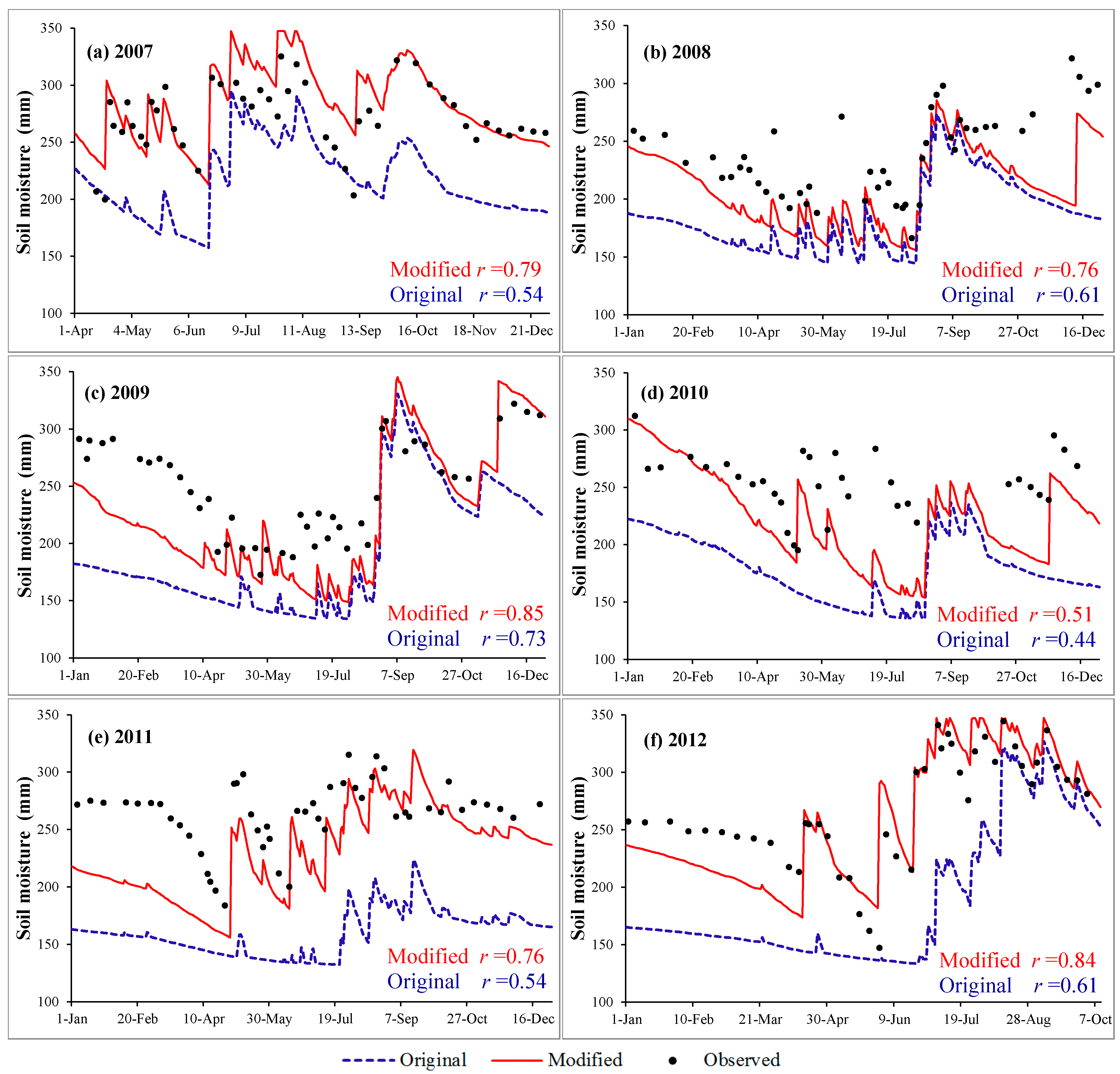
Comparing the farmland soil moisture in Luancheng station, the correlation coefficients between the results simulated by the modified model and the observed values from 2007 to 2012 were 0.73, 0.76, 0.85, 0.51, 0.76 and 0.84, respectively; which had increased by 32.7%, 24.6%, 16.4%, 15.9%, 40.7% and 37.7%, respectively, compared with the performance of the original method. It turned out that the simulation results were ideal and provided a more objective response to the farmland moisture-changing process.

(2)

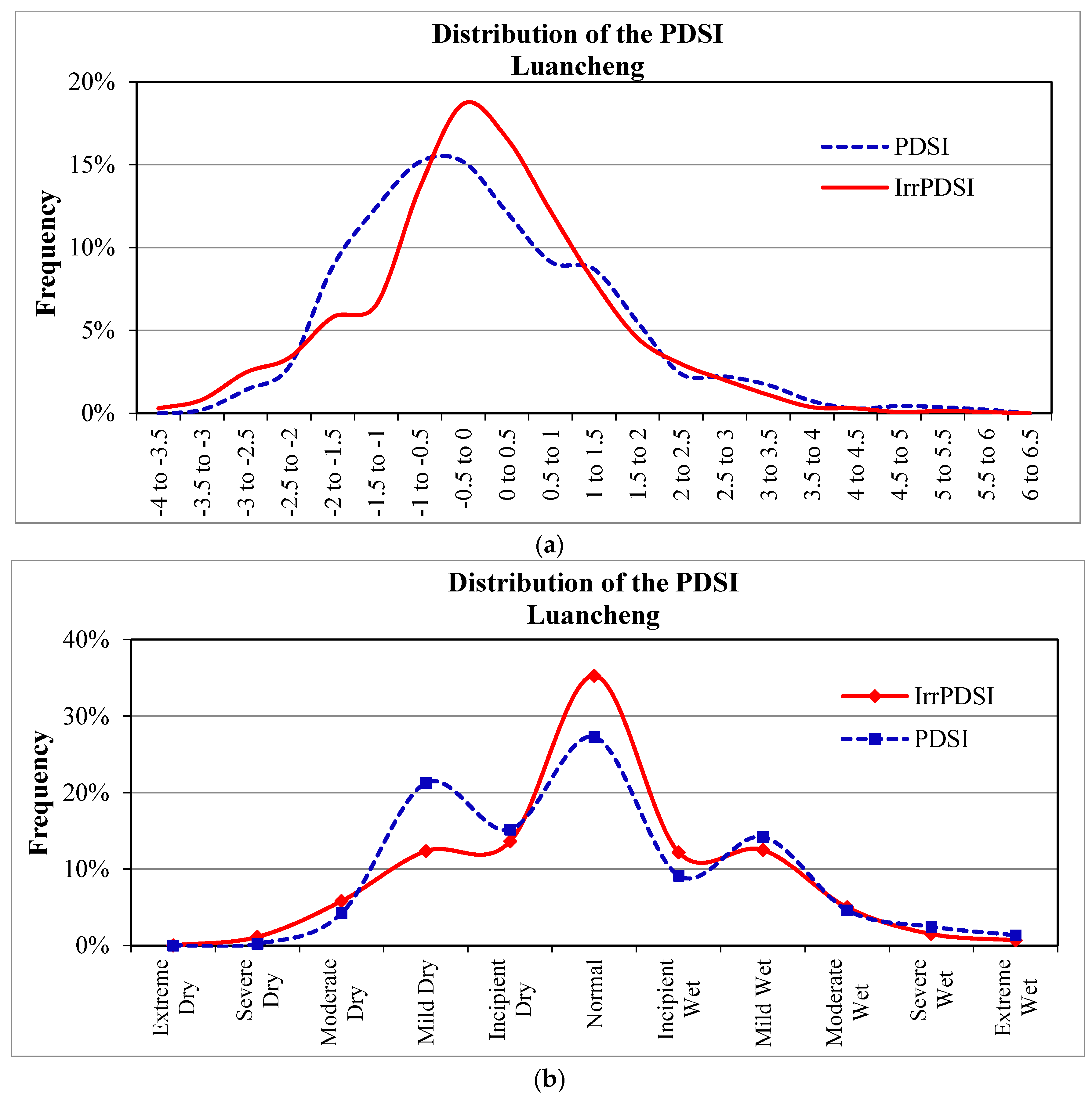
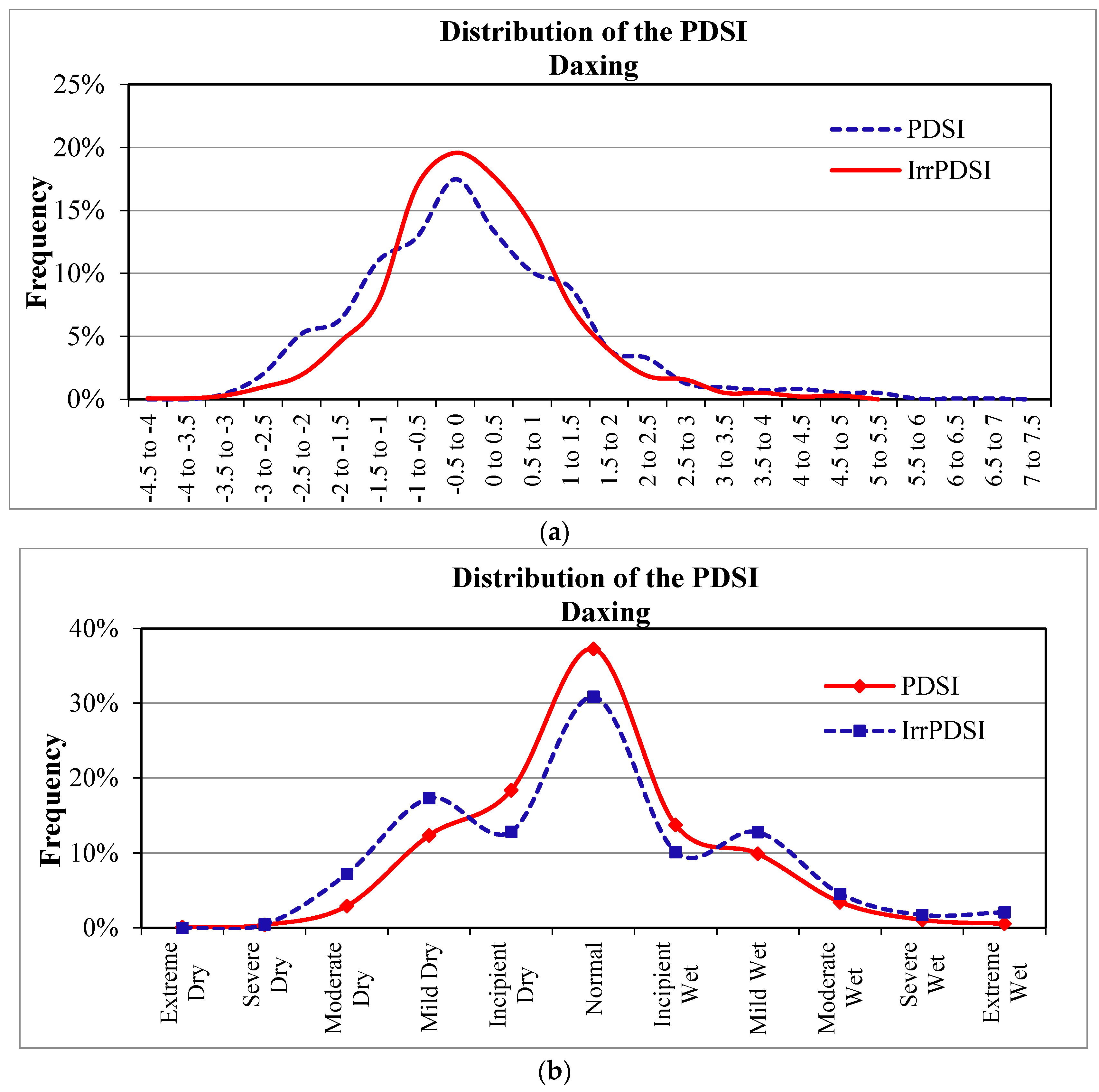
The statistical analyses indicated that the frequencies of mild dry and wet reported by the PDSI were 21% and 14% for Luancheng, and 17% and 13% for Daxing, respectively, which did not fit with the belief that the frequency of mild dry should be approximately equal to mild wet. Contrarily, the IrrPDSI reported a nearly normal distribution, and mild dry and wet occurred with a close frequency (12% for Luancheng and 10% for Daxing, respectively). Moreover, the results showed that 39 of the 47 stations in the study area based on IrrPDSI had nearly normal distributed values, whereas only half of the stations examined based on the PDSI did.

(3)

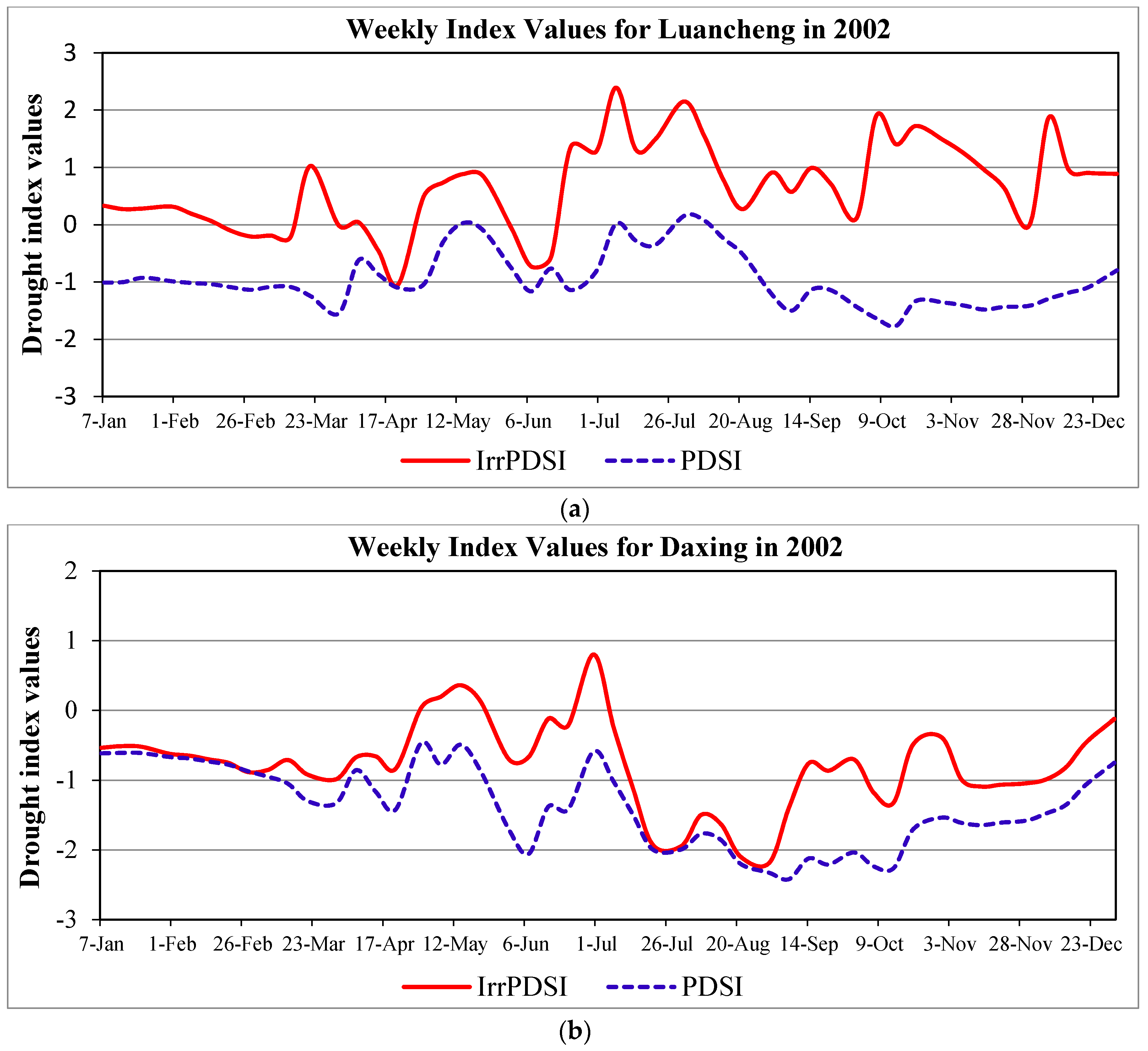
The time series plot of the two PDSIs showed that the IrrPDSI reported a normal or mild wet category in Luancheng station and incipient or mild dry in Daxing station during July and December 2002, respectively; whereas the PDSI reported more negative results than the IrrPDSI. The report of agricultural disasters confirmed that the results reported by the IrrPDSI were more consistent with the real conditions.

(4)

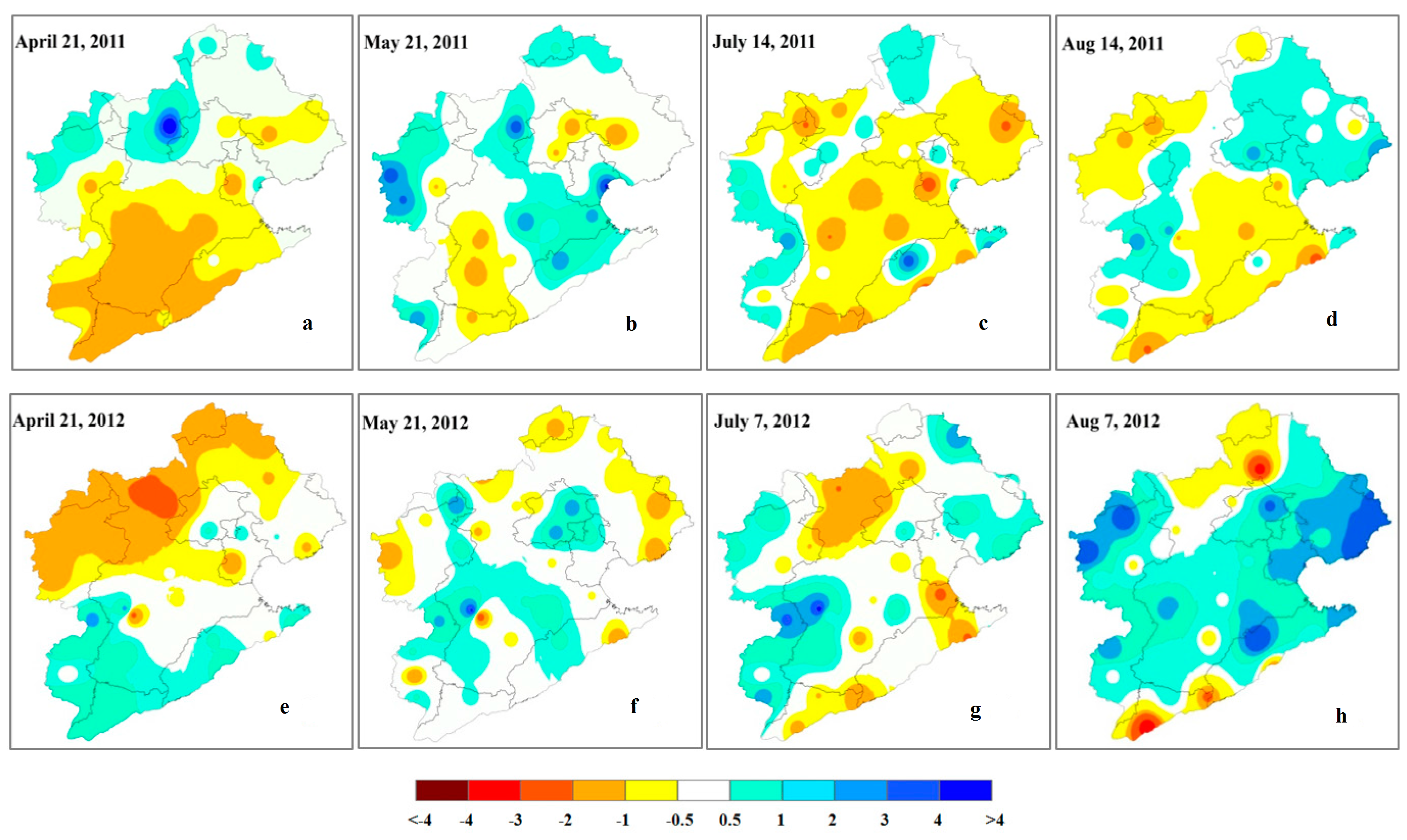
The spatial analyses showed that the results reported by IrrPDSI matched historical records better than the PDSI during the irrigated season, which showed that irrigation can usually effectively relieve drought conditions. There were insignificant differences between the distributions of dry–wet based on the two indices during the non-irrigated season as a result of infrequent irrigation.

Overall, the IrrPDSI performed well in assessing agricultural drought in the Haihe River Basin. This study is fairly preliminary and limited to the selected basin, and further research is needed before applying it elsewhere. First, the auto-irrigation threshold method may be innovative and general; however, the drought index formula in this article may be more applicable to arid, semi-arid and semi-humid regions such as north China, and also for regions with similar climates. As for different climatic zones, owing obviously to different irrigation schedules the assessed results might have some deviations. Therefore, the formula might need to make appropriate adjustments according to the local irrigation schedule. Second, there is uncertainty as to whether the index has an advantage over other agricultural drought indices, and more in-depth research is needed before a definitive conclusion can be reached. Third, irrigated areas accounted for most of the total cultivated land in the study area. For this reason, randomly scattered non-irrigated land was not taken into account in this work, and this also requires more exploration. Nonetheless, this work can meaningfully guide agricultural drought management in irrigated regions heavily disturbed by human activity.

References

- Masud, M.B.; Khaliq, M.N.; Wheater, H.S. Future changes to drought characteristics over the Canadian Prairie Provinces based on NARCCAP multi-RCM ensemble. Clim. Dyn. 2016, 48, 1–21. [Google Scholar] [CrossRef]
- Masud, M.B.; Khaliq, M.N.; Wheater, H.S. Analysis of meteorological droughts for the Saskatchewan River Basin using univariate and bivariate approaches. J. Hydrol. 2015, 522, 452–466. [Google Scholar] [CrossRef]
- Palmer, W.C. Meteorological Drought; Research Paper No. 45; U.S. Department of Commerce Weather Bureau: Washington, DC, USA, 1965.
- Palmer, W.C. Keeping track of crop moisture conditions, nationwide: The new Crop Moisture Index. Weather Wise 1968, 21, 156–161. [Google Scholar] [CrossRef]
- Shafer, B.A.; Dezman, L.E. Development of a Surface Water Supply Index (SWSI) to assess the severity of drought conditions in snowpack runoff areas. In Proceedings of the 50th Annual Western Snow Conference, Reno, NV, USA, 19 April 1982; Colorado State University: Fort Collins, CO, USA, 1982; pp. 164–175. [Google Scholar]
- Meyer, S.J.; Hubbard, K.G.; Wilhite, D.A. A crop-specific drought index for corn: I. Model development and validation. Agron. J. 1993, 85, 388–395. [Google Scholar] [CrossRef]
- Kogan, F.N. Droughts of the late 1980s in the United States as derived from NOAA polar-orbiting satellite data. Bull. Am. Meteorol. Soc. 1995, 76, 655–668. [Google Scholar] [CrossRef]
- Patel, N.R.; Chopra, P.; Dadhwal, V.K. Analyzing spatial patterns of meteorological drought using standardized precipitation index. Meteorol. Appl. 2007, 14, 329–336. [Google Scholar] [CrossRef]
- Narasimhan, B.; Srinivasan, R. Development and evaluation of Soil Moisture Deficit Index (SMDI) and Evapotranspiration Deficit Index (ETDI) for agricultural drought monitoring. Agric. For. Meteorol. 2005, 133, 69–88. [Google Scholar] [CrossRef]
- Hao, Z.; AghaKouchak, A. A nonparametric multivariate multi-index drought monitoring framework. J. Hydrometeorol. 2014, 15, 89–101. [Google Scholar] [CrossRef]
- Van Loon, A.F.; Gleeson, T.; Clark, J.; Van Dijk, A.I.; Stahl, K.; Hannaford, J.; Di Baldassarre, G.; Teuling, A.J.; Tallaksen, L.M.; Uijlenhoet, R.; et al. Drought in the Anthropocene. Nat. Geosci. 2016, 9, 89–91. [Google Scholar] [CrossRef]
- Sadri, S.; Kam, J.; Sheffield, J. Nonstationarity of low flows and their timing in the eastern United States. Hydrol. Earth Syst. Sci. 2016, 20, 633–649. [Google Scholar] [CrossRef]
- Wilhite, D.A.; Buchanan-Smith, M. Drought and Water Crises: Science, Technology, and Management Issues; CRC Press: Boca Raton, FL, USA, 2005; pp. 4–29. [Google Scholar]
- Hosseini, S.M.; Sharifzadeh, A.; Akbari, M. Causes, effects and management mechanisms of drought crisis in rural and nomadic communities in southeastern Iran as perceived by agricultural/rural managers and specialist. J. Hum. Ecol. 2009, 27, 189–200. [Google Scholar]
- Vicente-Serrano, S.M.; Beguería, S.; López-Moreno, J.I. Comment on “Characteristics and trends in various forms of the Palmer Drought Severity Index (PDSI) during 1900–2008” by Aiguo Dai. J. Geophys. Res. 2011, 116, D19112. [Google Scholar] [CrossRef]
- O’Farrell, P.J.; Anderson, P.M.L.; Milton, S.J.; Dean, W.R.J. Human response and adaptation to drought in the arid zone: Lessons from southern Africa. S. Afr. J. Sci. 2009, 105, 34–39. [Google Scholar]
- Wilhite, D.A. Drought as a natural hazard: Concepts and definitions. In Droughts: A Global Assesment; Routledge: London, UK, 2000; Volume 1, pp. 3–18. [Google Scholar]
- Li, Z.; Hao, Z.; Shi, X.; Déry, S.J.; Li, J.; Chen, S.; Li, Y. An agricultural drought index to incorporate the irrigation process and reservoir operations: A case study in the Tarim River Basin. Glob. Planet. Chang. 2016, 143, 10–20. [Google Scholar] [CrossRef]
- Mishra, A.K.; Ines, A.V.; Das, N.N.; Khedun, C.P.; Singh, V.P.; Sivakumar, B.; Hansen, J.W. Anatomy of a local-scale drought: Application of assimilated remote sensing products, crop model, and statistical methods to an agricultural drought study. J. Hydrol. 2015, 526, 15–29. [Google Scholar] [CrossRef]
- Sauer, T.; Havlík, P.; Schneider, U.A.; Schmid, E.; Kindermann, G.; Obersteiner, M. Agriculture and resource availability in a changing world: The role of irrigation. Water Resour. Res. 2010, 46, 666–669. [Google Scholar] [CrossRef]
- Portmann, F.T.; Siebert, S.; Döll, P. MIRCA2000—Global monthly irrigated and rainfed crop areas around the year 2000: A new high-resolution data set for agricultural and hydrological modeling. Glob. Biogeochem. Cycles 2010, 24, 2013–2024. [Google Scholar] [CrossRef]
- Narayanamoorthy, A. Development and composition of irrigation in India: Temporal trends and regional patterns. Irrig. Drain. 2011, 60, 431–445. [Google Scholar] [CrossRef]
- State Statistical Bureau. Statistical Yearbook; Statistical Press of China: Beijing, China, 2014. (In Chinese)
- Cao, X.; Wang, Y.; Wu, P.; Zhao, X.; Wang, J. An evaluation of the water utilization and grain production of irrigated and rain-fed croplands in China. Sci. Total Environ. 2015, 529, 10–20. [Google Scholar] [CrossRef] [PubMed]
- Van Loon, A.F.; Stahl, K.; Di Baldassarre, G.; Clark, J.; Rangecroft, S.; Wanders, N.; Gleeson, T.; Van Dijk, A.I.; Tallaksen, L.M.; Hannaford, J.; et al. Drought in a human-modified world: Reframing drought definitions, understanding, and analysis approaches. Hydrol. Earth Syst. Sci. 2016, 20, 3631–3650. [Google Scholar] [CrossRef]
- Vasiliades, L.; Loukas, A. Hydrological response to meteorological drought using the Palmer drought indices in Thessaly, Greece. Desalination 2009, 237, 3–21. [Google Scholar] [CrossRef]
- Sun, L.; Mitchell, S.W.; Davidson, A. Multiple drought indices for agricultural drought risk assessment on the Canadian prairies. Int. J. Climatol. 2012, 32, 1628–1639. [Google Scholar] [CrossRef]
- Gobena, A.K.; Gan, T.Y. Assessment of trends and possible climate change impacts on summer moisture availability in western Canada based on Metrics of the Palmer Drought Severity Index. J. Clim. 2013, 26, 4583–4595. [Google Scholar] [CrossRef]
- Yuan, S.; Quiring, S.M. Drought in the U.S. Great Plains (1980–2012): A sensitivity study using different methods for estimating potential evapotranspiration in the Palmer Drought Severity Index. J. Geophys. Res. 2014, 119, 10996–11010. [Google Scholar] [CrossRef]
- Tei, S.; Yonenobu, H.; Sugimoto, A.; Ohta, T.; Maximov, T.C. Reconstructed summer Palmer Drought Severity Index since 1850 AD based on δ 13 C of larch tree rings in eastern Siberia. J. Hydrol. 2015, 529, 442–448. [Google Scholar] [CrossRef]
- Zou, L.; Xia, J.; She, D. Drought characteristic analysis based on an improved PDSI in the Wei River Basin of China. Water 2017, 9, 178. [Google Scholar] [CrossRef]
- Alley, W.M. The Palmer Drought Severity Index: Limitations and assumptions. J. Appl. Meteorol. 1984, 23, 1100–1109. [Google Scholar] [CrossRef]
- Mishra, A.K.; Singh, V.P. A review of drought concepts. J. Hydrol. 2010, 391, 202–216. [Google Scholar] [CrossRef]
- Sepulcrecanto, G.; Horion, S.; Singleton, A. Development of a combined drought indicator to detect agricultural drought in Europe. Nat. Hazards Earth Syst. Sci. 2012, 12, 3519–3531. [Google Scholar] [CrossRef]
- Quiring, S.M.; Papakryiakou, T.N. An evaluation of agricultural drought indices for the Canadian prairies. Agric. For. Meteorol. 2003, 118, 49–62. [Google Scholar] [CrossRef]
- Ye, J.; Shen, S.; Lu, H. Application of modified palmer drought severity index in agricultural drought monitoring. Chin. J. Agro-Meteorol. 2009, 30, 257–261. (In Chinese) [Google Scholar]
- Cai, Y.; Wang, M.; Zhou, Z.; Chen, D.; Zhang, Y. Palmer drought severity model and its application in Mianyang. Plateau Mt. Meteorol. Res. 2010, 30, 55–59. (In Chinese) [Google Scholar]
- Mika, J.; Horváth, S.; Makra, L.; Dunkel, Z. The palmer drought severity index (PDSI) as an indicator of soil moisture. Phys. Chem. Earth Parts A/B/C 2005, 30, 223–230. [Google Scholar] [CrossRef]
- Dai, A. Drought under global warming: A review. WIREs Clim. Chang. 2011, 3, 45–65. [Google Scholar] [CrossRef]
- Ren, X.S.; Hu, Z.L.; Cao, Y.B.; He, S. Water Resources Assessment in the Haihe River Basin; Water Resources and Electricity Press: Beijing, China, 2007. (In Chinese) [Google Scholar]
- Fang, Q.X.; Ma, L.; Green, T.R.; Yu, Q.; Wang, T.D.; Ahuja, L.R. Water resources and water use efficiency in the North China plain: Current status and agronomic management options. Agric. Water Manag. 2010, 97, 1102–1116. [Google Scholar] [CrossRef]
- Chen, S.; Li, R. Assessment of surface water resources and evapotranspiration in the Haihe River Basin of China using SWAT model. Hydrol. Process. 2013, 27, 1200–1222. [Google Scholar]
- Gao, G.; Xu, C.Y.; Chen, D.; Singh, V.P. Spatial and temporal characteristics of actual evapotranspiration over Haihe River Basin in China. Stoch. Environ. Res. Risk Assess. 2012, 26, 1–15. [Google Scholar] [CrossRef]
- Wells, N.; Goddard, S. A self-calibrating palmer drought severity index. J. Clim. 2004, 17, 2335–2351. [Google Scholar] [CrossRef]
- Liu, Z.; Yan, A.L.; Qiao, C.L. Research on application of palmer drought model in Jinghuiqu irrigation area. Agric. Res. Arid Areas 2010, 28, 259–264. (In Chinese) [Google Scholar]
- Xiao, J.F.; Liu, Z.D.; Liu, X.F.; Liu, Z.G.; Chen, Y.M. Analysis and study on irrigation problem of main spring maize area of China. Water Sav. Irrig. 2010, 4, 1–3. (In Chinese) [Google Scholar]
- Water Industry Standard of the People’s Republic of China (SL568-2012): Soil Moisture Evaluation; Ministry of Water Resources of PRC: Beijing, China, 2012. (In Chinese)
- Gu, R.; Tang, Z. Analysis of the cause of drought in Shandong in the summer 2002. Meteorol. Mon. 2004, 30, 22–26. (In Chinese) [Google Scholar]
- Zou, X.; Zhai, P.; Zhang, Q. Variations in droughts over China: 1951–2003. Geophys. Res. Lett. 2005, 32, 353–368. [Google Scholar] [CrossRef]
- Xue, D.; Wang, J.; Wang, X. Characteristic analysis of change into drought in Shandong Province. J. Nat. Disasters 2007, 16, 60–65. (In Chinese) [Google Scholar]