Article

Influence of Rack Slope and Approaching Conditions in Bottom Intake Systems

Hidr@m Group, Department of Civil Engineering, Universidad Politécnica de Cartagena, Paseo Alfonso XIII, 52, 30203 Cartagena, Spain
*
Author to whom correspondence should be addressed.
Water 2017, 9(1), 65; https://doi.org/10.3390/w9010065
Submission received: 7 December 2016 / Revised: 12 January 2017 / Accepted: 16 January 2017 / Published: 21 January 2017
(This article belongs to the Special Issue Modeling of Water Systems)

Abstract

:
The study analyzes the flow over bottom racks made of longitudinal T-shaped bars. A clear water flow is considered in a laboratory flume. Free surface profiles, wetted rack lengths, and discharge coefficients are measured, changing parameters such as longitudinal slope, void ratio, and approaching flow. The present work complements existing experimental studies, considering the influence of the approaching flow conditions. The velocity field measured with Particle Image Velocimetry (PIV) technique and the pressure field with Pitot tubes are quantified. Numerical simulations (CFD) are used to complement laboratory data. The energy head along the rack is calculated and compared with the hypothesis of horizontal energy level with minimum energy at the beginning of the rack. A discharge coefficient adjustment that considers the slope, the void ratio, and the position along the rack is proposed and presented with the results of other works. Theoretical proposals to calculate the pressure field along the flow are compared with measurements in the laboratory. The relation between the static pressure head in the space of bars and the discharge coefficient is used as an alternative method to define the discharge.

1. Introduction

Bottom intake systems made by racks and longitudinally disposed in the flow direction are classically used to derive mean flows in continuous mountains rivers with intensive sediment transport. Nowadays, work is ongoing to study these intakes in order to derive flash floods from ephemeral rivers in semi-arid zones, not to control flooding but to collect runoff and improve the availability of resources. Several authors have proposed design recommendations to avoid rack occlusion from prototype observations in mountain rivers (e.g., Orth et al. [1]; Ract-Madoux et al. [2]; Krochin [3]; Drobir [4]; Bouvard [5]; Raudkivi [6]). Castillo et al. [7], from experimental measurements in a flow with gravel-sized materials, found that a longitudinal rack slope around 30% minimizes the occlusion effect.
The wetted rack length to derive a flow yields very different results depending on the study. This is due to the variation in the experimental conditions used to adjust the discharge coefficient, such as the shape of the bars, their separation and width, the void ratio (the ratio between the spacing between bars, b1, and the total area, b1 + bw, where bw is the bar width), and the approaching flow conditions such as the initial flow depth, h1, or the longitudinal rack slope, tanθ.
In the static discharge coefficient, Cq0, obtained with null approaching velocity, the influence of the first two factors can be observed (Noseda [8], Brunella et al. [9], Righetti and Lanzoni [10]).
The longitudinal rack slope has been considered in several ways (see formulations included in Appendix A). While some authors confirm the influence of the slope on the efficiency of the rack and in the wetted rack length (Garot [11]; Orth [1]; White et al. [12]; Righetti and Lanzoni [10]), other researchers experimentally found that there is no further influence for slopes steeper than 19° (Brunella et al. [9]).
Figure 1 shows the dimensionless ratios between the wetted rack length to critical flow depth, L/hc, in function of the specific approaching flow and the Froude number at the beginning of the rack, q1/Fr1. Formulae consider the void ratio m = 0.60, and a longitudinal slope of 20%. Expressions assume the simplification of horizontal energy level or constant specific energy, not considering the possible energy losses along the rack. Differences between formulae are mainly due to the shape of the bars. For the T-shaped case and the prismatic plane bars, the dimensionless wetted rack length is 3.20–3.70 (Frank [13], Drobir [4], Bouvard and Kunztmann [14], Krochin [3], Noseda [8]). However, in circular or prismatic rounded bars the dimensionless wetted rack length is 1.98–2.87 (Brunella et al. [9], Righetti and Lanzoni [10], Vargas [15]).
In Figure 1, there are also some field measurements obtained by Drobir [16] in a prototype made with circular bars, and complemented by a laboratory scale model leading to a potential adjustment that envelops the maximum wetted length over the bar, L2, and the maximum wetted length in the space between bars, L1. The length proposed by the free overfall, in the case of a horizontal channel that ends in a brink (around 1.4) is also presented (Henderson [17]). Krochin [3] introduces the f factor to consider the percentage of rack that is occluded (see Appendix A). In Figure 1 no occlusion has been considered (f = 0).
According to Figure 1, the shape of the bars, the spacing between them, and the inlet conditions have to be taken into account when the designers estimate the discharge coefficient and the wetted rack length.
The flow over bottom intake systems is three-dimensional and spatially varied, presenting interactions with bottom bars and high turbulence level. As a simplification, the discharge coefficient is usually adjusted with the hypothesis of no dissipation energy along the rack (horizontal energy head, Figure 2c), one-dimensional and hydrostatic pressure distribution. Using the orifice equation (Equation (1)), considering that derived flow will be subtracted from the principal flow, and the derivative of the energy equation (Equation (2)), the water surface profile may be obtained (Equation (3)):
d q d x = C q H m 2 g ( H 0 + x sin θ )
H 0 + x sin θ = h + U 2 2 g
d h d x = 2 m C q H ( H 0 + x sin θ ) ( H 0 + x sin θ h cos θ ) + h sin θ 3 h cos θ 2 ( H 0 + x sin θ ) ,
where CqH is the discharge coefficient considering the energy height in the orifice equation, H0 the energy height at the beginning of the rack, x the longitudinal coordinate in the rack plane, θ the angle between the bottom rack and the horizontal, m the void ratio, h the flow depth along the rack, and g the gravitational acceleration.
Equation (3) can be solved by a numerically fourth-order Runge–Kutta algorithm with two boundary conditions, the flow depth, h1, at the inlet section and the approaching flow, q1. With these assumptions, Brunella et al. [9] proposed an adjustment to calculate the flow profile along the bottom rack for longitudinal slopes steeper than 19° (34.4%).
Several authors experimentally verified differences of the pressure field from the hydrostatic conditions in flows along the rack (Mostkow [18]; Venkataraman [19]; Nasser et al. [20,21]; Ramamurthy and Satish [22]; Righetti et al. [23]). The results of Melik-Nubarow [24], cited by Krochin [3], relate the vertical velocity component in the slit between two bars with the static pressure:
U y , s l i t = 2 g ( P s l i t γ ) ,
where Uy,slit and Pslit are the perpendicular component of the velocity vector and the static pressure in the slit, respectively (Figure 2c).
Replacing Equation (4) in Equation (1), the discharge coefficient may be calculated from the static pressure in the slit, Pslit, and using a contraction coefficient, Cc, to consider the effective area:
d q d x = C q H m 2 g H = U y , s l i t C c m = 2 g ( P s l i t γ ) C c m
C q H = ( P s l i t H γ ) C c .
Nakagawa [25] and Castro-Orgaz and Hager [26] proposed obtaining the pressure field from the equations of continuity and Euler perpendicular to the rack plane. The longitudinal component of the velocity may be assumed to be constant or proportional to the mean velocity in each section.
The present work takes into consideration the approaching conditions of the flow and the longitudinal slope of the bottom intakes. The computational fluid dynamics (CFD) simulations are used as a complement to the laboratory measurements. Combining an extensive experimental campaign with CFD simulations, the main flow parameters are analyzed for subcritical approaching flows.
These results complement the existing studies carried out by different authors (see Table 1).

2. Materials and Methods

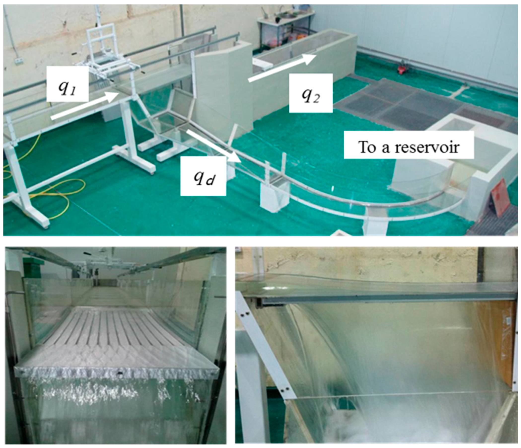
2.1. Laboratory Flume

The laboratory measurements were carried out in a laboratory flume with an inlet channel 5.00 m long, 0.50 m wide, and 0.40 m high. The channel ends in a bottom rack with a variable slope from 0% to 33% (0 to 18.26°) (see Figure 3). Flows derived and rejected are collected by two different channels. Flow aligners are installed upstream of the inlet channel to ensure uniform conditions along the approaching channel. The approaching flow in the physical device is subcritical in all the cases at the beginning of the inlet channel. The flow reaches supercritical conditions at the beginning of the rack. Brunella et al. [9] proposed an expression to calculate the critical Reynolds number in the bottom intake system cases. According to those authors, there are no scaling effects when this value is bigger than 250,000. In the tests carried out, the critical Reynolds number was between 287,000 and 678,000. Following [9], no scale effects are expected.
The inlet flow rates are measured by an electromagnetic flowmeter of 125 mm Endress Häuser Promag 53 W with an error of 0.5% of the full scale. The rejected flow rates are measured by a 90° V-notch weir. The collected or derived flows are obtained as a difference between them. Further details on the experimental setup can be found in García [27]. During the tests the water temperature was between 18 and 19.5 °C.
To measure the derived flow per unit of length, a movable plate of 1 mm thickness was placed over the rack. The plate allowed us to increase the rack length from 0 to 90 cm. Since the flow along the rack is supercritical, the distortion that occurs at the rack and plate junction is a very local phenomenon. Thus, the derived flow was obtained as the difference between the total inlet flow and rejected flow.
The racks are formed of T-shaped (T 30/25/2 mm, see Figure 2b) bars, with a length of 0.90 m and disposed longitudinally. Three different spacings are adopted, which generate three different rack settings. Table 2 summarizes the geometric characteristics of each rack, where bw is the width of the bars. This table includes the flow characteristics of the 60 tests carried out, such as: flow depth, h1, energy head at the beginning of the rack, H0, Froude number at the beginning of the rack, Fr1, and ratio of the flow rejected at the end of the 0.90 m length rack, q2, to the approaching flow, q1. The ratio of q2/q1 below 4% usually corresponds to the flow rejected through the top part of the planar bars. The Froude numbers at the beginning of the rack grow from horizontal to 33% rack slopes, adopting values from 1.28 to 2.08. The range Fr1 obtained in the tests is representative of the flow conditions found in intermediate and steep slope rivers. Vargas [15] and Drobir [16] are examples of direct applications of the Froude modeling in two steep slope rivers, where the Froude numbers agree with the range studied.
In Table 3, the approaching flow depth related to critical depth, h/hc, is presented at a cross section located x = −0.50 m upstream of the rack. As values are close to the unit, this zone is where the flow profile starts to decrease.

2.2. Instruments

A vertical point gauge with an accuracy of 0.5 mm was used to measure the free surface flow profile.
The velocity field was measured with a Particle Image Velocimetry (PIV) system. This consisted of a high-speed camera Motion Pro HS-3 (DEL Imaging Systems, LLC, Cheshire, CT, USA), a zoom lens with 12.5/75 mm focal length, lens aperture f/11, 520 × 520 pixels resolution, 8 bits → 255 shades and a distance from the camera to stream recorded of 0.50 m. Hence, the recording window dimensions were 9 cm × 9 cm. The laser was an Oxford Lasers Ltd. Firefly (Oxford Lasers, Inc., Shirley, MA, USA) 200 W, 808 nm high-speed imaging laser whose configuration was: pulse = 10 μs; beam width = 5.5 mm and power peak = 200 watts; 30 μs delay; wavelength 808 nm. The speed camera used is 600 Hz; 0.00017 (m/pixel).
The flow was seeded with polyamide particles of 50 μm size PSP-50 from Dantec Dynamics A/S (Skovlunde, Denmark). Frames were analyzed in consecutive pairs by cross-correlation algorithm in an interrogation area of 64 × 64 pixels with sub-windows of 32 × 32 pixels in a single pass search and overlapping of 50% (Adrian and Westerweel [28]).
Particle image diameter, including diffraction, is around 4 pixels, avoiding pixel-locking. No background slide subtraction or noise remove techniques were applied.
Spurious vectors technique based on reference velocity was used: the average of eight neighbors was calculated.
The PIVlab 1.41 software was used for the cross-correlation. This program is an open-source time-resolved particle image velocimetry tool in MATLAB® (Thielicke and Stamhuis [29]). In each test 80,000 images were recorded. The velocity values were averaged. The longitudinal velocity fluctuation turbulence intensity was around 0.04–0.15, increasing from the bottom.
The total pressure was measured with a Pitot tube tip placed in two different inclinations, 0 and 22° (Mostkow [18], García [27]). Signals were collected in a Rosemount™ (Chanhassen, MN, USA) 2051 pressure transmitter, with a differential pressure range of −62.2 to 62.2 mbar and an accuracy of 0.065% of the full scale (precision of 0.5 mm). Values were stored in a recorder/data logger with 50 Hz frequency from 4/20 mA analog signals. Time-averaged values were obtained as:
p t , β = ( h y ) + Δ P ρ g + U β 2 2 g + y ,
where β is the angle of the Pitot tube with the horizontal plane, h the flow depth in the x longitudinal coordinate, pt the total pressure (dynamic and static) registered by the Pitot tube in the β direction, ΔP the deviation of the pressure from hydrostatic, Uβ the velocity component in the β direction, and y the perpendicular coordinate.

2.3. Numerical Simulations

The clear water hydraulic behavior of the racks has also been analyzed with computational fluid dynamics (CFD) simulations. The laboratory data were used to estimate the accuracy of the simulations. These codes solve the differential Reynolds-Averaged Navier–Stokes (RANS) equations to satisfy the balance of the governing equations in the three directions. The main equations (mass and momentum conservations) may be written as:
ρ t + x j ( ρ U j ) = 0
ρ U i t + x j ( ρ U i U j ) = p x i + x j ( 2 μ S i j ρ u i u j ¯ ) ,
where xi defines the coordinate directions (i = 1 to 3 for x, y, z directions, respectively), t the time, ρ the flow density, p the pressure, U the velocity vector, u i the turbulent velocity, Sij the mean strain-rate tensor, μ the molecular viscosity, and ρ u i u j ¯ is the Reynolds stress (ANSYS Inc. [30]).
Due to the uncertainty of the numerical simulations, it is necessary to carry out a numerical uncertainty analysis (Celik et al. [31], Valero and Bung [32]).
The volume finite ANSYS CFX code (ANSYS Inc. [30]) was selected. Following previous simulations of intake systems and sensitivity analysis of the turbulence models (Castillo et al. [33,34,35,36]), the shear stress transport (SST) model was used to solve the closure problem of the RANS equations. This model takes into account the accuracy of the k-ω model in the near-wall region and the free stream independence of the k–ε model in the outer part of the boundary layer (Menter [37]). The homogeneous model was selected to solve air–water flow. The free surface was considered as an iso-surface on the 0.50 air volume ratio. The fluid domain consisted of three bars and two spacings. The boundary conditions were the flow and the turbulent kinetic energy (measured with a Acoustic Doppler Velocimeter (Nortek AS, Bærum, Norway) probe) at the inlet, the water depths and hydrostatic pressures distributions. For the water-collected channel, an opening boundary condition was used. In the vertical plane of the extreme bars, symmetry conditions and hexahedral elements were used in the simulations. Details of the numerical simulation can be found in Castillo et al. [7,35]. Figure 4 compares the flow profiles measured in laboratory over the center of the bars with the simulated data obtained for two mesh sizes. In all the cases, the water profiles obtained with the CDF methodology were similar to the lab measurements. There were no outstanding differences between the results obtained with the 0.004 and 0.002 m mesh sizes. However, the solver mean required time was around 5.5 times longer with the finer mesh size. For this reason, the 0.004 m mesh size was used to analyze the different specific flows and rack slopes.

2.4. Experimental and Numerical Campaign

Tests were made with specific flows q1 = 53.80; 77.00; 114.60 and 155.40 L/s/m for racks A, B, and C (m = 0.16, 0.22, and 0.28, respectively); and five longitudinal rack slopes: 0, 10%, 20%, 30%, and 33%. This entails 20 tests per rack. In each case, the free-surface flow profile and the flow derived per unit of length were measured. The total wetted rack length and the rejected flow at the end of the rack were also analyzed. Table 2 also shows the range of Froude number, Fr1, total head H0, and flow depth measured at the beginning of the rack in the experiments.
For rack C (m = 0.28), with horizontal and 30% slopes, the velocity and pressure fields were measured with PIV and Pitot tube instrumentations for three specific flows (q1 = 77.00; 114.60 and 138.80 L/s/m).

3. Results and Discussion

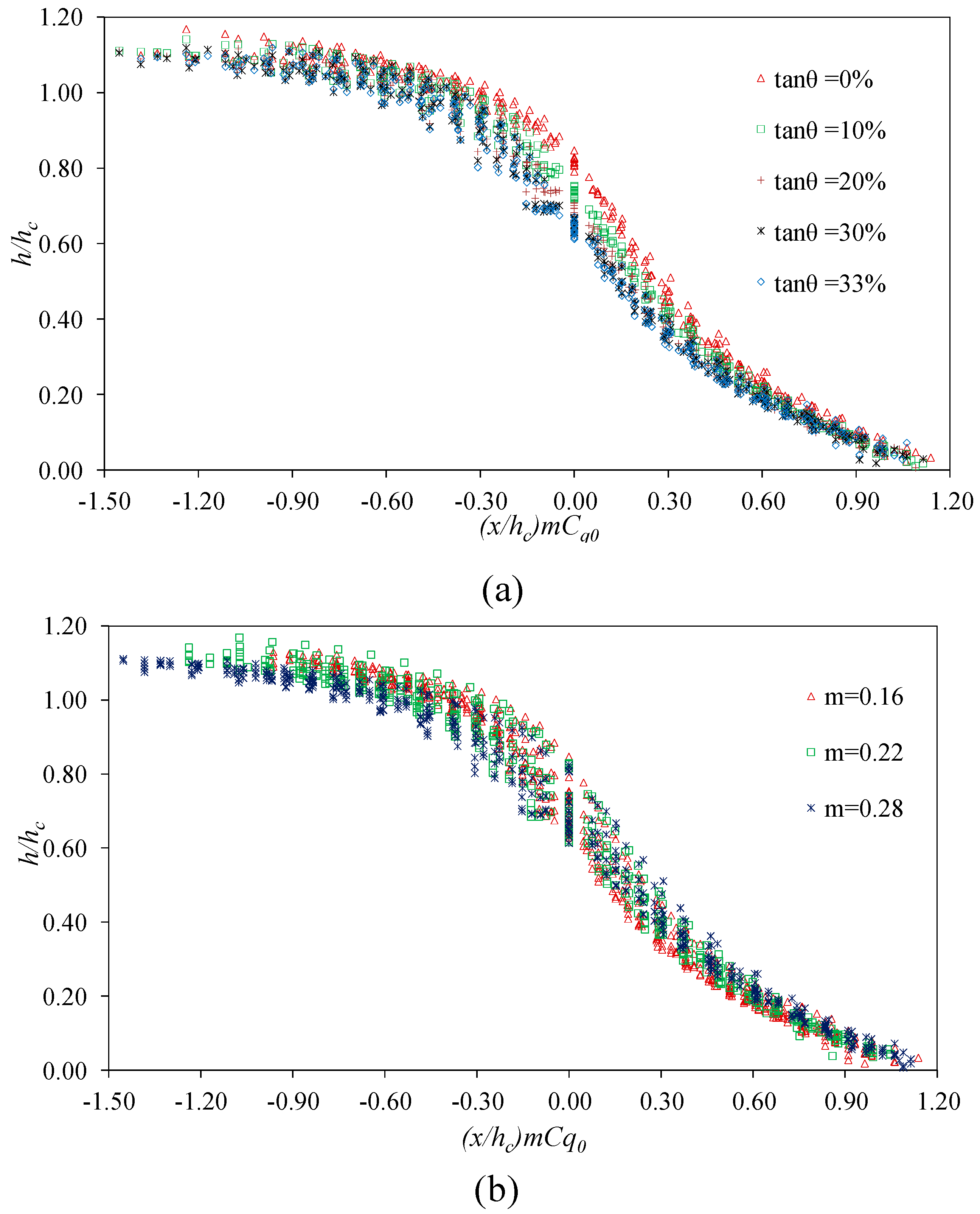
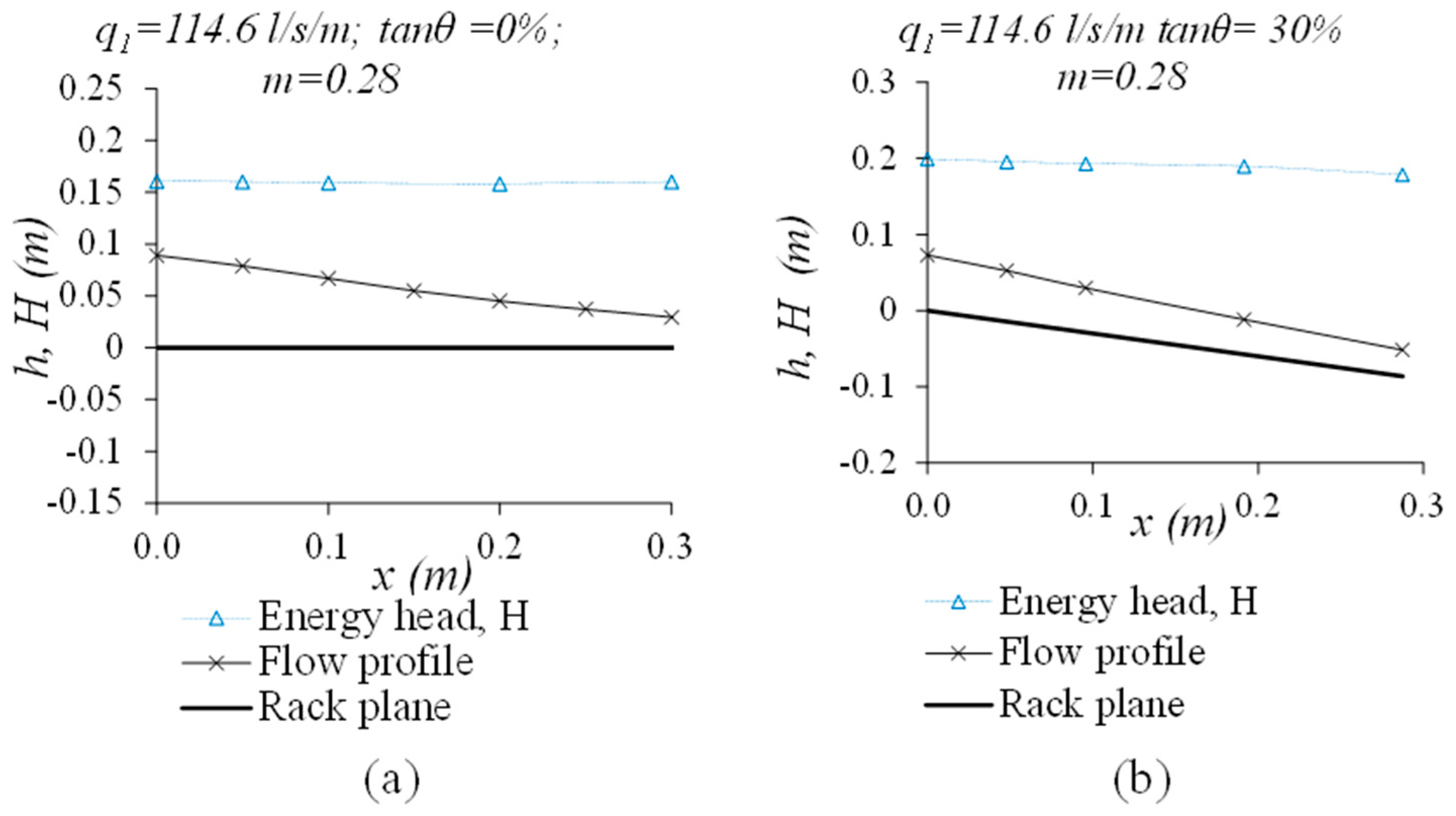
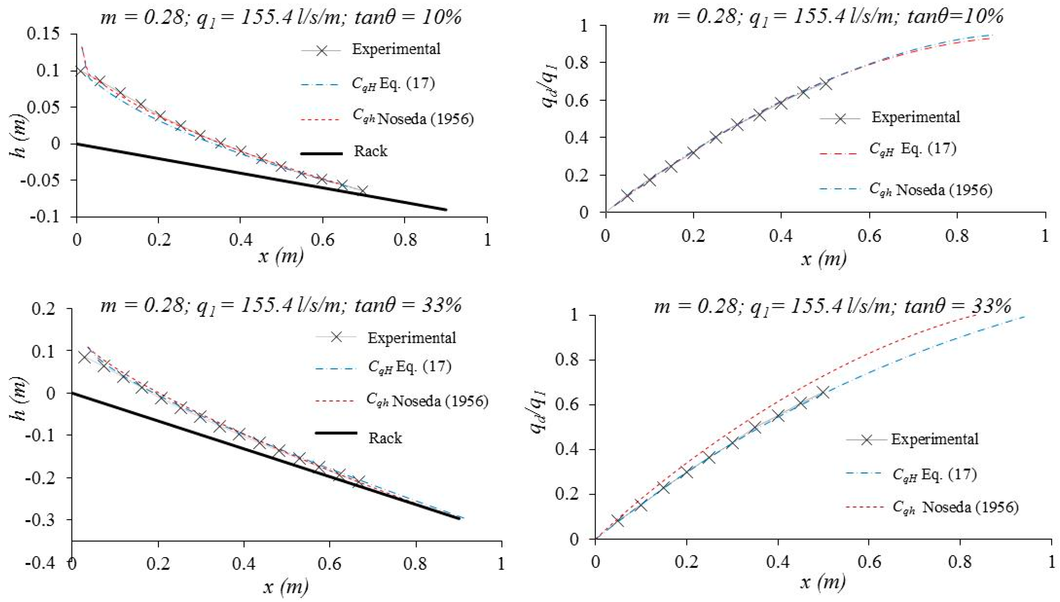
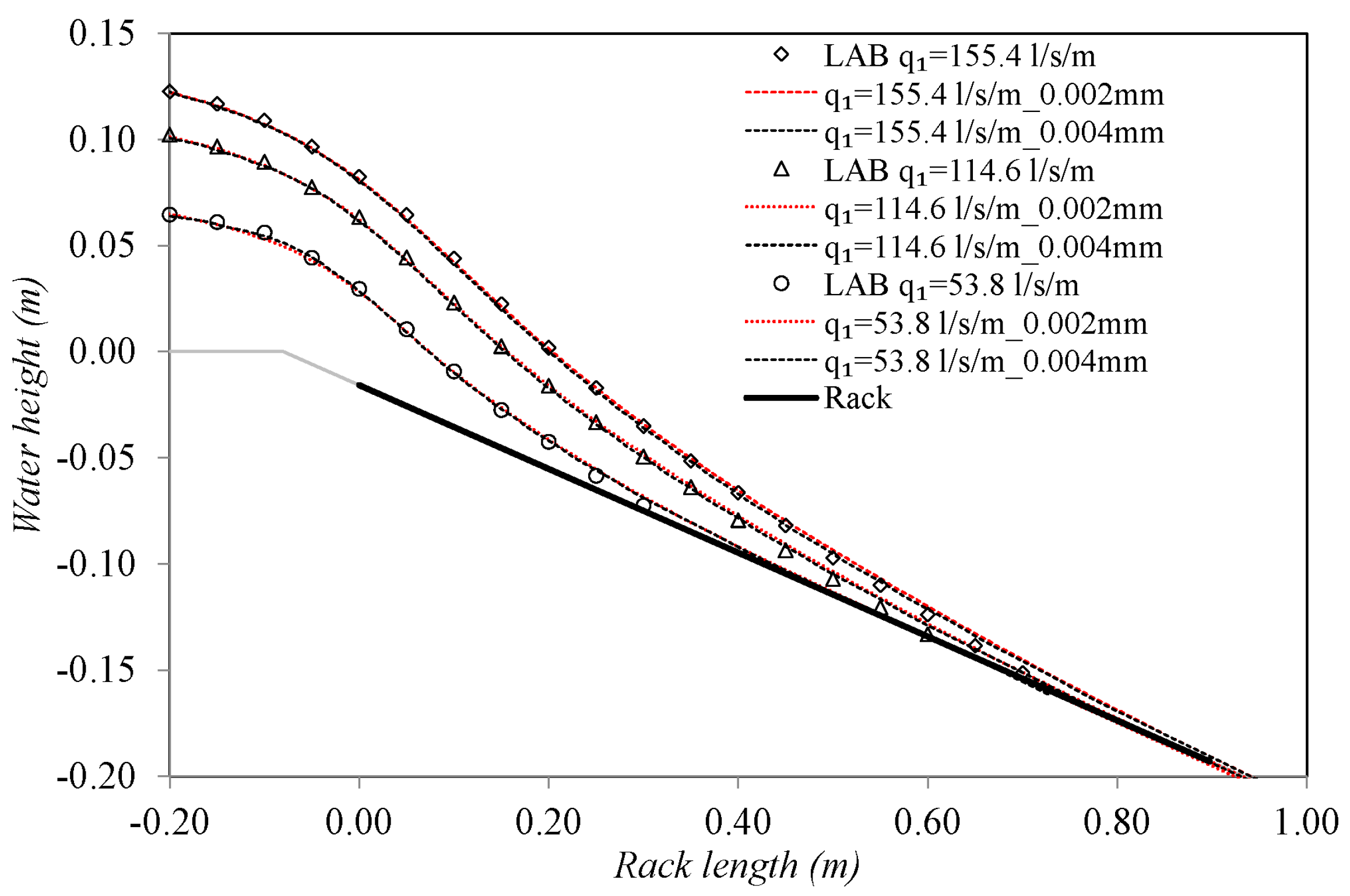
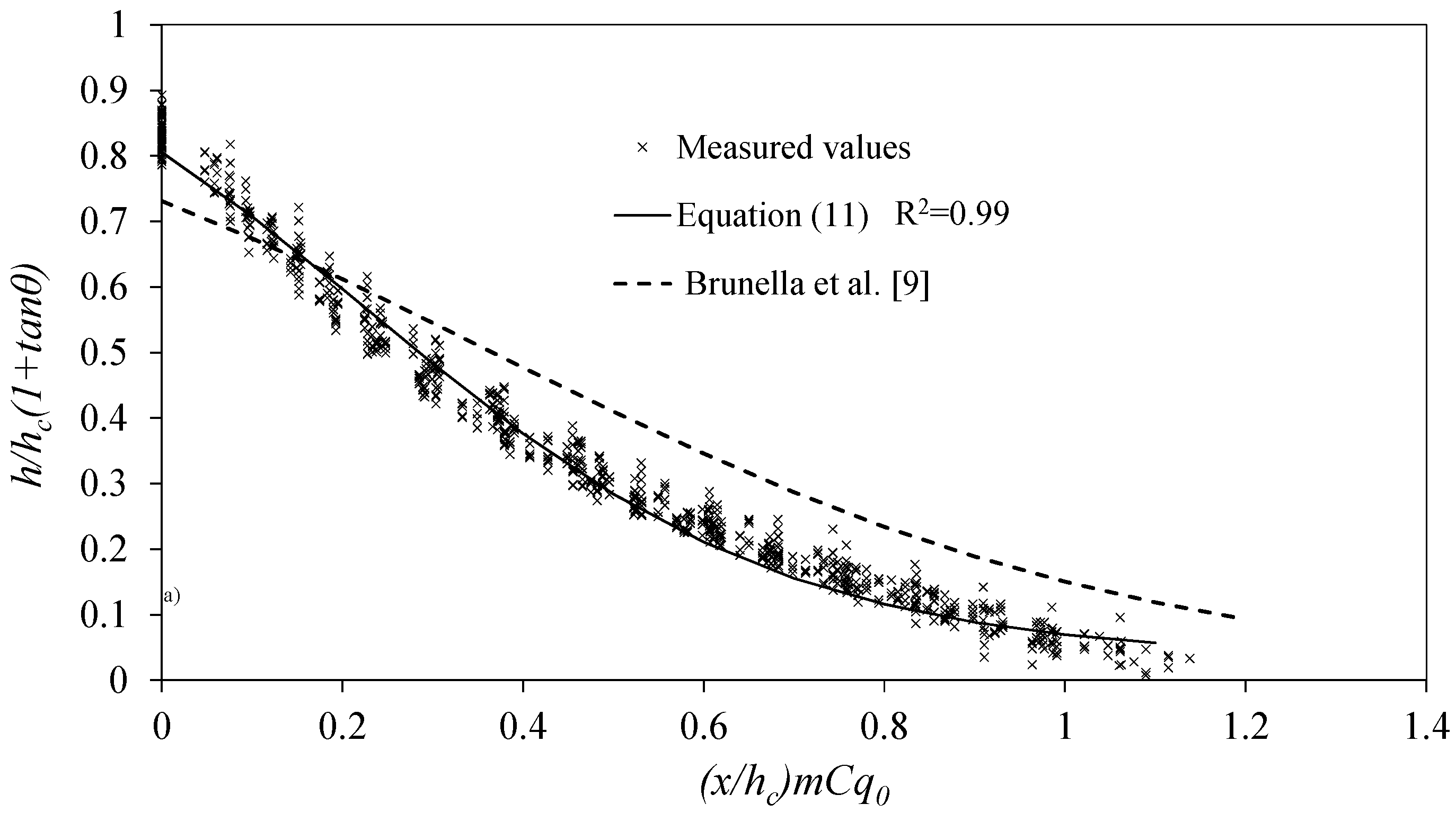
3.1. Free Surface Flow Profile

Flow depth perpendicular to the bottom of the rack, h, was measured each 0.05 m along the rack, from around 0.70 m upstream of the beginning of the rack to the end of the wetted rack. The zero value is located at the beginning of the rack. Four different approaching flows, three different void ratios, and five different slopes are considered.
Following Brunella et al. [9], the dimensionless free-surface flow profiles are presented in Figure 5 as a function of tanθ and the void ratio m, respectively. Differences in the water depth due to the slope variation are significant around the beginning of the rack (horizontal axis ≈ 0).
The static discharge coefficient, Cq0, was measured in a laboratory with a rack length of 0.30 m and placing a vertical wall at the end of the rack. Further details of how to measure the static discharge coefficient can be found in [8,9]. Therefore, the kinetic energy becomes potential and the Froude number of the approaching flow, Fr1, tends to 0. Figure 6a shows the values obtained for several approaching flows as a function of the void ratio. Figure 6b compares the averaged values of the static discharge coefficient, Cq0, calculated for each void ratio using T-shaped bars with those obtained by Garot [11], Noseda [8], Brunella et al. [9], and Righetti and Lanzoni [10] testing different shaped bars. In accordance with the results, an exponential adjustment of the Cq0 value is proposed as a function of the rack shape:
C q 0 = a exp 0.77 m ,
where a is a factor that depends on the shape of the bars: 1.43 for circular bars, 1.15 for prismatic rounded bars, and 0.90 for T-shaped bars.
By multiplying the h/hc value by the (1 + tanθ) factor, data adjust to a single curve over the rack.
h h c ( 1 + tan θ ) = 0.56 ( 1 tanh ( x 0.46 h c m C q 0 0.505 ) 0.94 )
Figure 7 shows the Brunella et al. [9] original expression, and the adjustment obtained in the present work for several longitudinal slopes (from 0% to 33%). The values measured in the laboratory have a correlation of R2 = 0.99 with Equation (11).

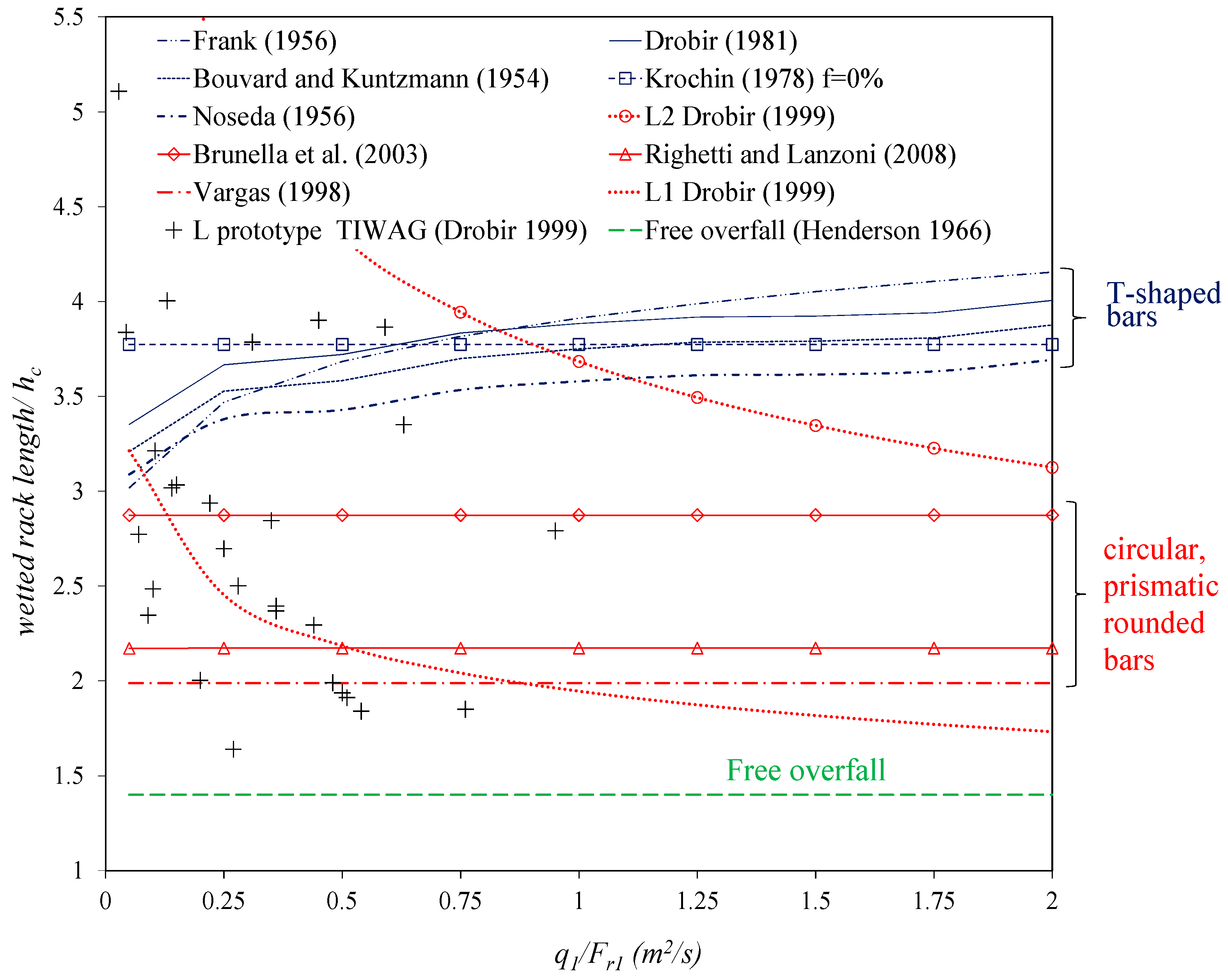
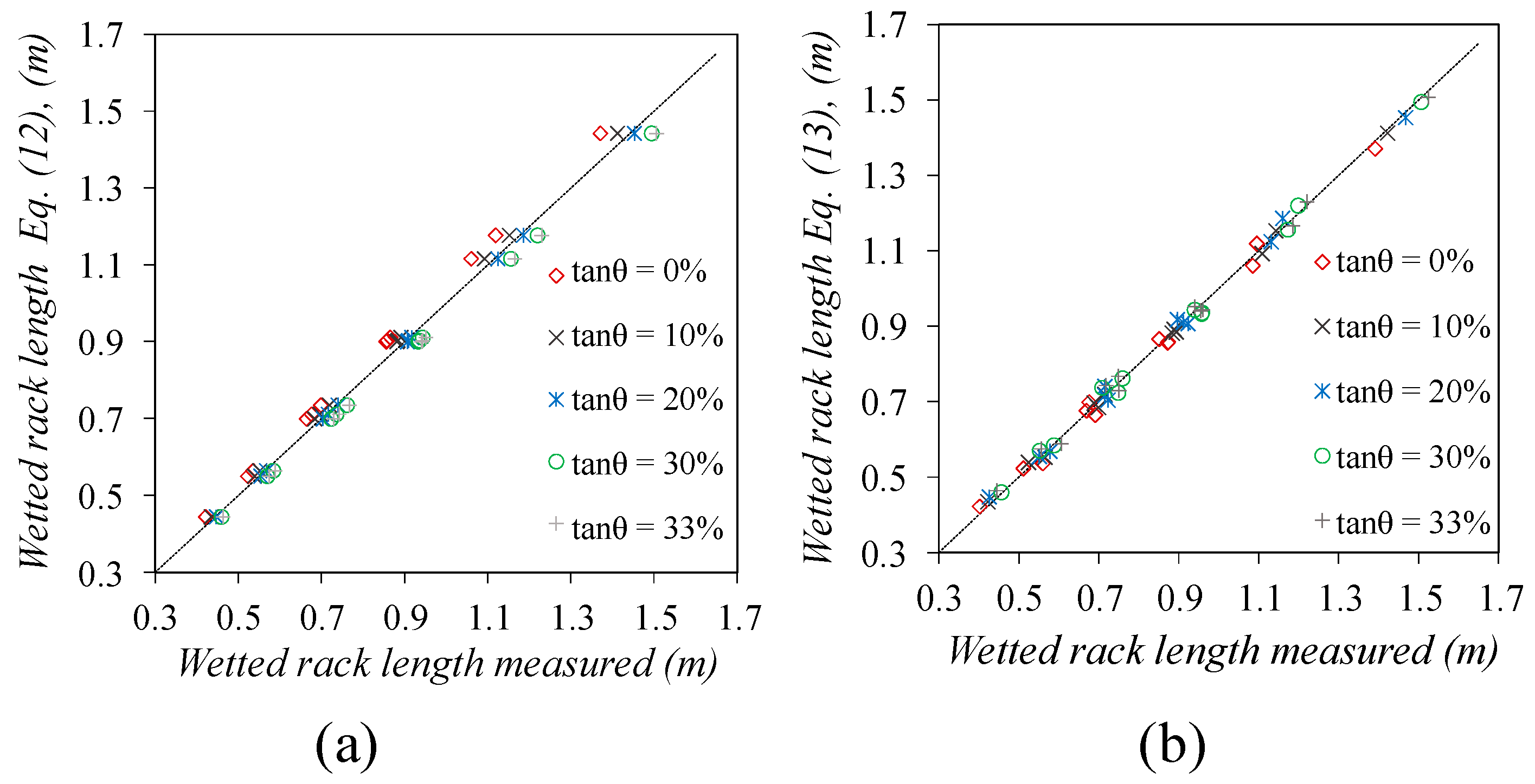
3.2. Wetted Rack Length

The maximum length of the flow in the slit, L1, measured in the laboratory adjusts to the values that Brunella et al. [9] considered as wetted length (see Figure 5 and Figure 7). However, the wetted rack length for T-shaped bars, L2, measured over the rack presents the influence of the rack slope.
Noseda [8] proposed an expression to estimate the required wetted rack length with slopes smaller than 20%:
L w e t t e d 1.1848 H 0 C q h m .
To estimate the required wetted rack length for all slopes, considering slopes up to 33%, the following expression is proposed:
L w e t t e d 1.3 h c m C q 0 ( 1 + 0.3 tan θ ) .
Wetted rack lengths measured in lab and calculated with Equations (12) and (13) are presented in Figure 8. Equation (12) is calculated with the hypothesis of H0 = Hmin, while Cqh is the average of the discharge coefficient values along the rack (calculated as 1.3 times the static discharge coefficient, Cq0, with a good approximation).
Equation (12) under-predicts wetted lengths with slopes higher than 20% and overestimates the required length for the lower slopes. A better agreement is obtained with Equation (13), which takes the rack slope into account.

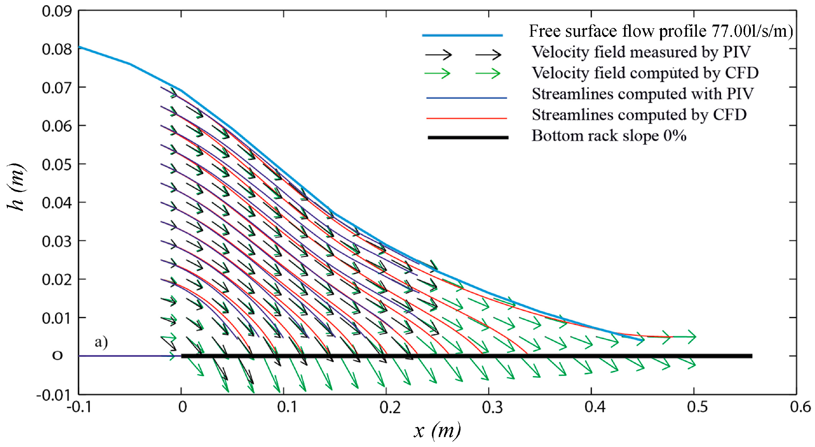
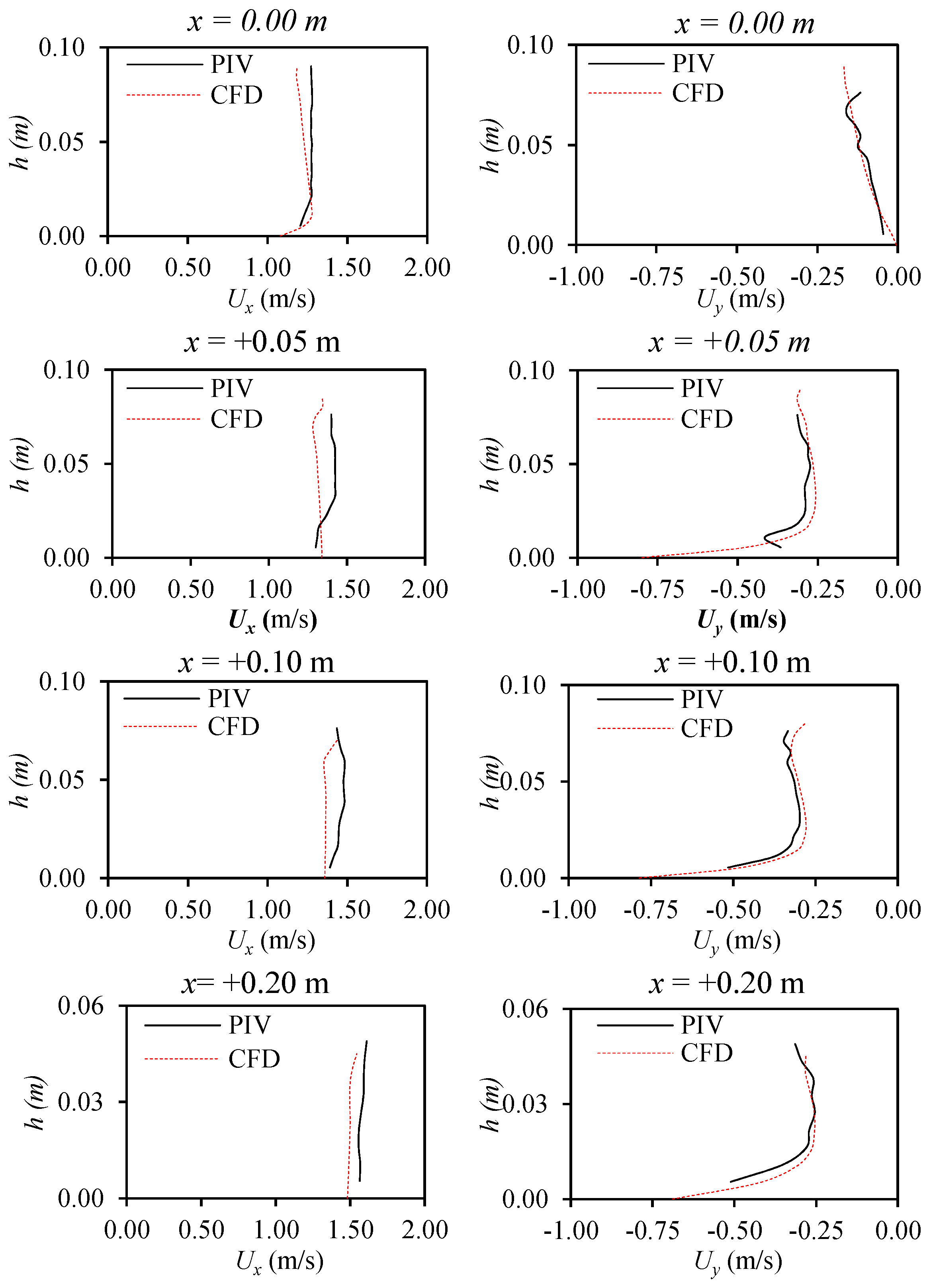
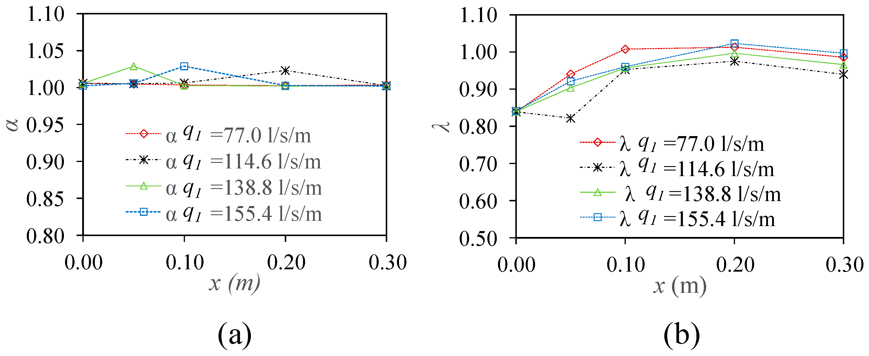
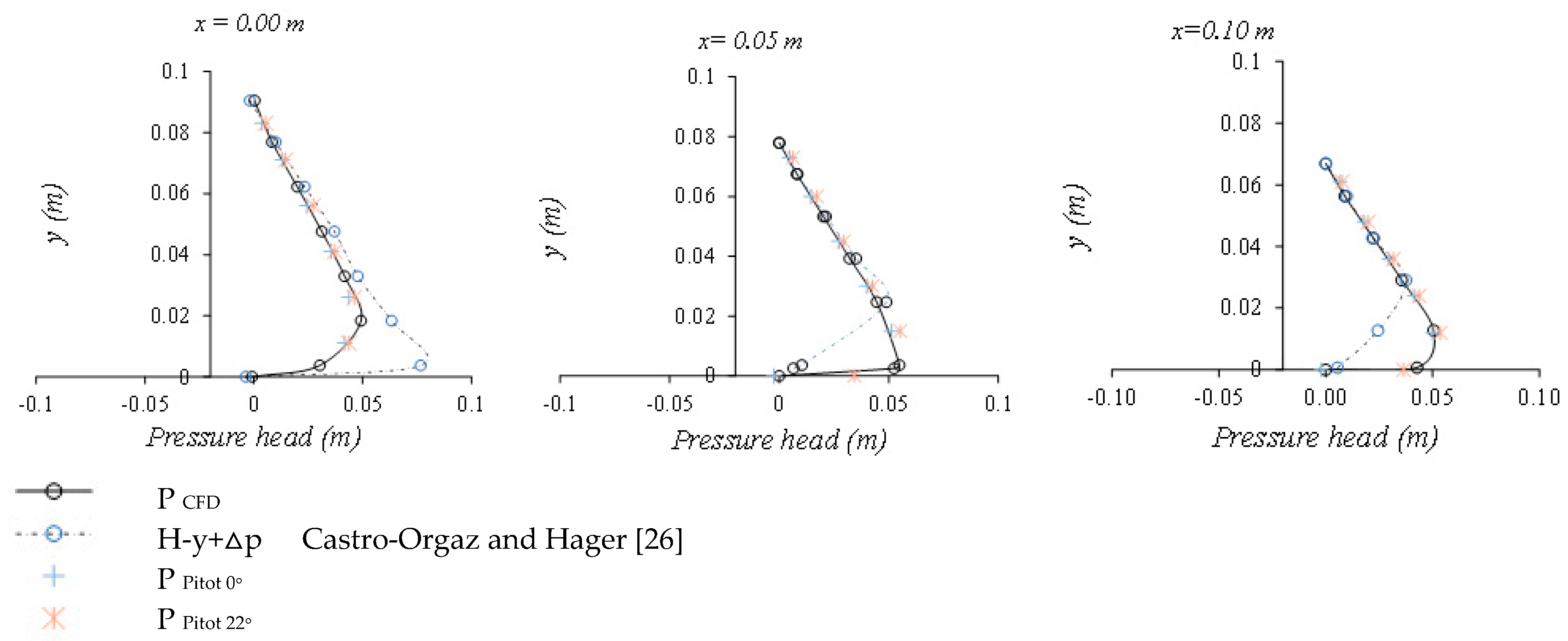
3.3. Velocity and Pressure Fields over the Rack

The flow over the rack of void ratio m = 0.28 has been measured with Particle Image Velocimetry (PIV). This instrumentation allows us to calculate the velocity field and the streamlines in a longitudinal plane located in the center of the slit between two bars. Values have been compared with the CFD simulations and a good agreement was achieved (Figure 9).
In Figure 10, the left plots refer to the longitudinal component of the velocity, Ux, while the right plots refer to the perpendicular velocity component, Uy. Values are compared in several sections along the rack (x = 0.00, 0.05, 0.10, and 0.20 m). The maximum differences in the longitudinal velocity component, Ux, are around 0.10 m/s, (<7%). For the perpendicular velocity component, Uy, differences are around 0.025 m/s, (<5%).
From the velocity field and the water depth, the energy level along the rack may be calculated using the Bernoulli equation. Figure 11 shows the flow profile and the energy level for q1 = 114.60 L/s/m, and slopes of 0% and 30%. The energy level starts with values over the minimum energy (water flow depths smaller than the critical depth). For the 0% slope, the energy level remains horizontal. However, the dissipation through the rack is around 0.10 m/m for the 30% rack slope.
Figure 12 shows the velocity and pressure coefficients of the energy equation, α and λ respectively, calculated from the following equations:
α = U i 3 d A U 3 A
λ = 1 q h [ P γ + y ] u d A ,
where Ui is the module of the velocity vector located in the position i, U the mean velocity vector in the section analyzed, q the flow along the rack in the x coordinate, and P the static pressure in the y coordinate.
The velocity coefficient α has values between 1.00 and 1.03 for all the flow rates analyzed. The pressure coefficient λ starts with values around 0.84 at the beginning of the rack, confirming the departure from hydrostatic conditions. At the end of the rack, λ tends to values around the unit.
The effect of these factors in the estimation of the flow profile and the flow derived per unit of length is usually included in the discharge coefficient. If these coefficients are considered, for the horizontal case, Equation (2) would become:
d h d x = d λ d x h 2 + 2 C q H m α ( H λ h ) H d α d x h ( H λ h ) α 3 λ h 2 H .
From the total pressure field measured by Pitot tubes, pt,β, and using the velocity field measured with the PIV system, the static pressure in the flow is calculated from Equation (4). Figure 13 shows the values for the approaching flow q1 = 114.60 L/s/m, horizontal slope, and several longitudinal coordinates. The static pressure measured with Pitot tubes inclined 0° and 22° approximates to the numerically simulated values.
Differences between them appear in the vicinity of the slit, where the 0° inclination values start to diverge from the 22° measurements and the simulated data. Results are in agreement with those presented by Katchatrian [38], cited by Mostkow [18].
Figure 13 also shows the pressure field along the rack obtained from the theoretical proposal of Castro-Orgaz and Hager [26], where Δp is the theoretical deviation from the hydrostatic values. The three methods are quite similar in the upper part of the flow, while the values present divergence in the vicinity of the slit.

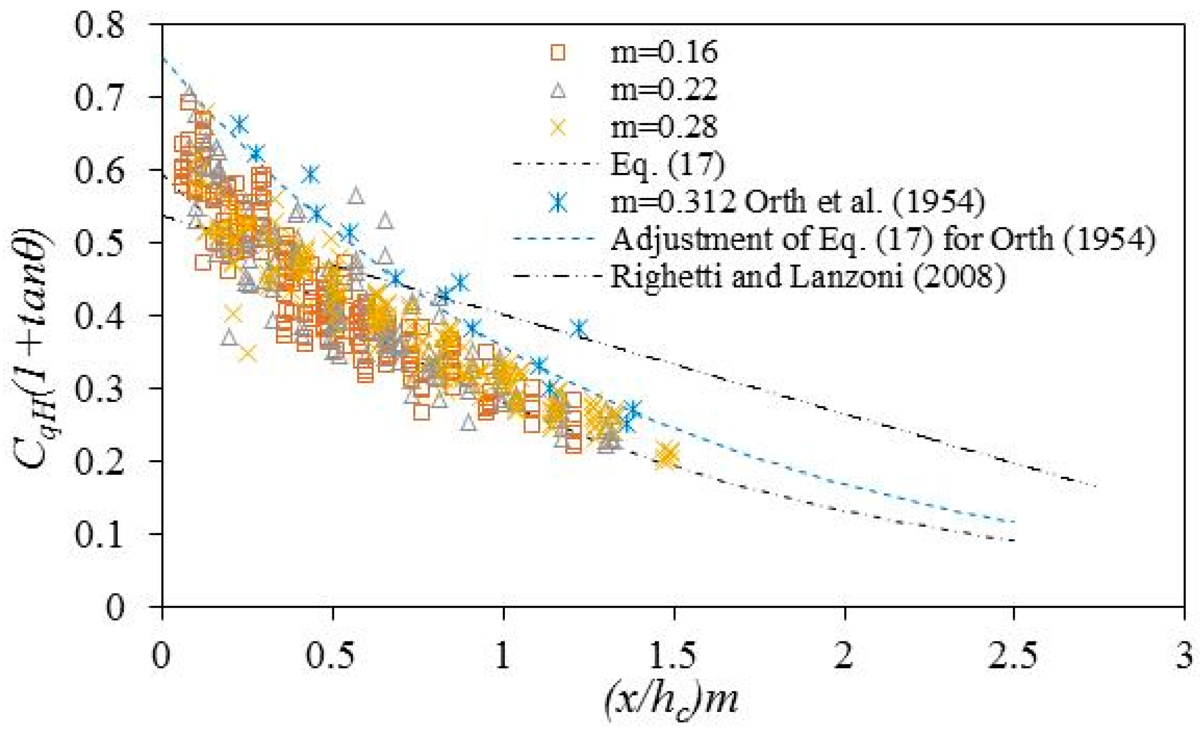
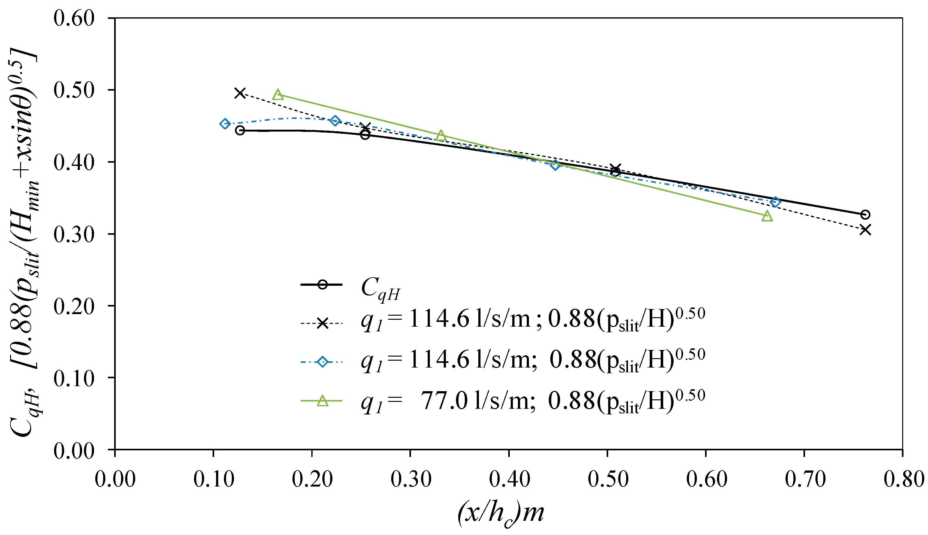
3.4. Discharge Coefficient

The derived flow per unit of length was measured in the laboratory. From Equation (1), the discharge coefficient may be obtained with the hypothesis of H0 = Hmin. The CqH values are influenced by the void ratio and the slope. Lower values are obtained for the higher slopes and void ratios. In all the cases, the coefficient decreases as the flow moves along the rack. Figure 14 presents the CqH multiplied by the factor (1 + tanθ), which allows us to estimate a unique adjustment. Considering the results, an exponential equation is proposed to calculate the discharge coefficient along the rack, as a function of rack slope:
C q H 0.58 e 0.75 ( x h c m ) ( 1 + 0.9 tan θ ) .
This equation considers three parameters, as did the expressions proposed by Righetti and Lanzoni [10] and Righetti et al. [23].
However, Equation (17) takes into account the longitudinal rack slope instead of the parameter FH0 at the beginning of the rack (see Appendix A).
Figure 14 also shows the values measured in laboratory by Orth et al. [1] for a hydrodynamic profile. To adjust the discharge coefficient, the first coefficient from Equation (17) has been modified from 0.58 to 0.75. The discharge coefficient proposed by Righetti and Lanzoni [10] is also presented for the case of q1 = 155.40 L/s/m and horizontal slope.
From Equations (1), (2) and (17), the flow profile and the derived flow per unit of length may be calculated. Figure 15 shows the case of q1 = 155.40 L/s/m, T-shaped bars, m = 0.28, and 0 and 33% rack slopes. Laboratory data are compared with the values proposed by Noseda [8] for the discharge coefficient included in the Appendix A, and with the numerical resolution of the following equations:
d q d x = C q h ( h ) m 2 g h
d h d x = 2 m C q h ( h ) h cos θ ( H 0 h cos θ ) 3 h cos θ 2 ( H 0 ) .
For small slope cases, the measured values adjust to that calculated. For the 33% slope case, differences appear with the Noseda [8] values. These variations are due to the fact that Noseda did not consider the longitudinal slope of the rack, and the author studied the discharge coefficient with rack slopes from the horizontal to 20%.
From another point of view, Righetti and Lanzoni [10] and Righetti et al. [23] experimentally checked the analogy between the discharge coefficient from Equation (1) and the sine of the angle of the velocity vector with the plane of the rack. They used the PIV equipment with racks made by top rounded bars of Plexiglas with a spacing of 2 mm. The void ratio m = 0.28, with four specific flows and two slopes, has been considered as an example. Figure 16 shows a comparison of the discharge coefficient calculated from Equation (1) with the energy head defined by the PIV measurements (Figure 10) and the sine of the angle of the velocity vector with the plane of the rack simulated with CFD. Although the experiments are different from those analyzed by Righetti and Lanzoni, the analogy between CqH and the sine of the angle of the velocity vector seems clear.
From Equations (1) and (4), we can find a different procedure to obtain the discharge coefficient, CqH. From the velocity and pressure fields, the static pressure head in the slit may be obtained. A contraction coefficient has to be experimentally adjusted. If the horizontal energy level with initial value equal to minimum energy is considered, then an additional coefficient K needs to be introduced:
C q H C c p s l i t H C c K p s l i t H min + x sin θ .
In Figure 17, the values of the discharge coefficient along the rack, defined by Equation (1), have been compared with those obtained from Equation (20). For the case of a horizontal slope and a void ratio m = 0.28, the contraction coefficient obtained is CcK ≈ 0.88.

4. Conclusions

This study complements previous works (Noseda [8], Brunella et al. [9], Righetti and Lanzoni [10]) in bottom intake systems with T-shaped bars disposed longitudinally.
Noseda’s [8] experimental campaign ranged from horizontal to 20% slopes. The current study has been done with the same type of racks as Noseda. It presents experimental values for slopes from horizontal to 33%, complementing existing works.
Brunella et al. [9] carried out measurements with circular bars. They found no influence of the rack slope for angles bigger than 19°. In this study, the measurements are taken for angles up to 18.26° (33% slope). The adjustments of the flow profile and wetted rack length can be compared with the results of Brunella et al. [9].
From the values obtained by Brunella et al. [9], Righetti and Lanzoni [10], and our own values, an adjustment of the static discharge coefficient is proposed. This adjustment considers different bar profiles and void ratios that give a vision of the range of this parameter.
Numerical simulations show good agreement with experimental measurements in the case of velocity and pressure field (Figure 10 and Figure 13), and discharge coefficient (Figure 16). In this way, numerical simulations are used as a complement to the experimental measurements.
An exponential adjustment to calculate CqH(x) has been proposed in Equation (17). Following Righetti and Lanzoni [10], the discharge coefficient has been compared with the sine of the angle of the velocity vector in the slit. The results show good agreement.
The energy head along the rack has been calculated, obtaining an energy loss around 0.10 m/m for 30% slopes. Differences from the hydrostatic pressure are observed along the rack. From the static pressure measurements, the discharge coefficient may be calculated through Equation (20). This can be considered as an alternative way of estimating the discharge coefficient (Figure 17).

Acknowledgments

The authors are grateful for the financial support received from the Seneca Foundation of Región de Murcia (Spain) through the project “Optimización de los sistemas de captación de fondo para zonas semiáridas y caudales con alto contenido de sedimentos. Definición de los parámetros de diseño”. Reference: 19490/PI/14.

Author Contributions

Luis G. Castillo carried out the analysis and application of the methodology, provided the application case study, analyzed the results, and participated in the writing. Juan T. García carried out the laboratory measurements, the data treatment, and participated in the writing. José M. Carrillo carried out the numerical simulations and participated in the writing. All three authors reviewed and contributed to the final manuscript.

Conflicts of Interest

The authors declare no conflict of interest.

Abbreviations

aconstant depending on the shape of bars in Equation (10);
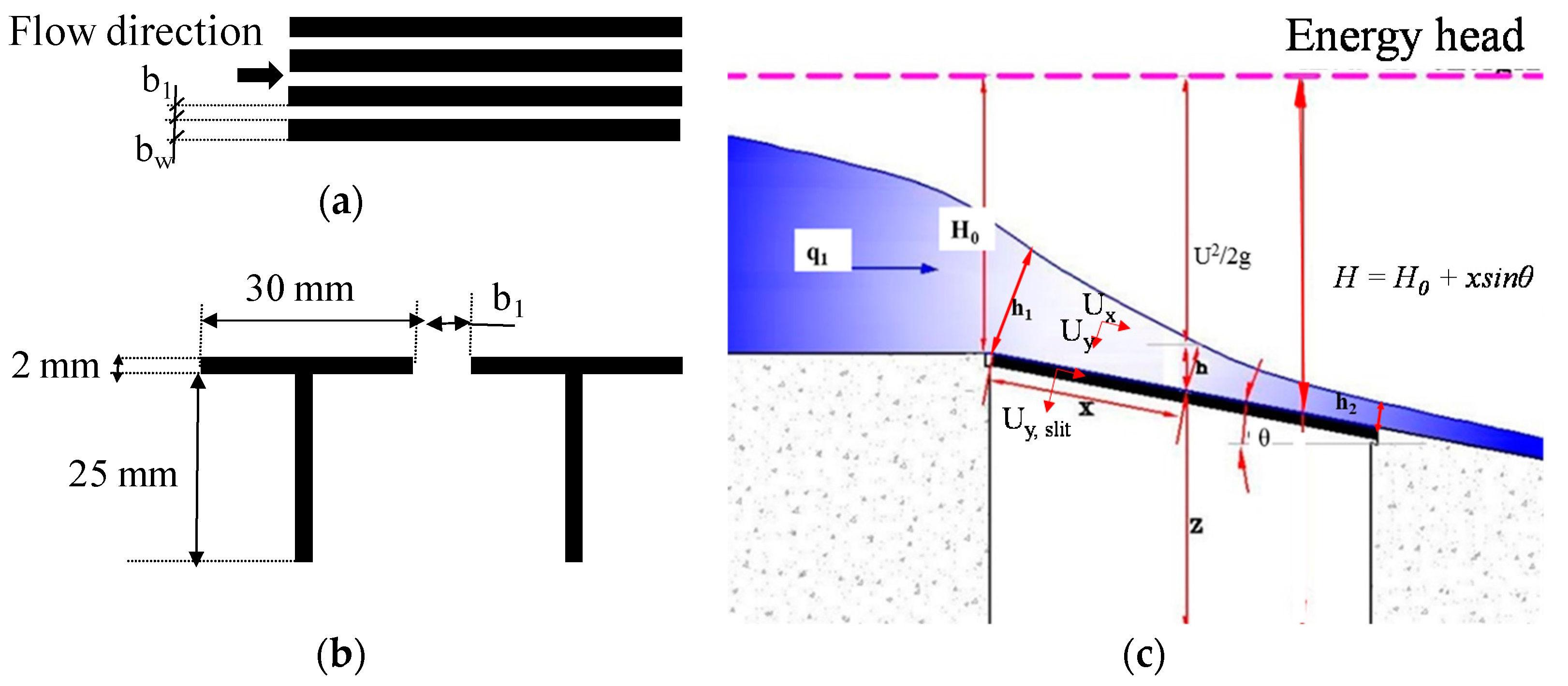
b1space between bars;
bwbar width;
Cccontraction coefficient for effective flow area;
CqHdischarge coefficient for energy head;
Cqhdischarge coefficient for flow depth;
Cq0static discharge coefficient;
fpercentage of occluded rack in Equation of Krochin [3] included in Appendix A;
ggravitational acceleration;
Henergy head along the rack referred to the rack plane;
H0energy head at the beginning of the rack referred to the rack plane;
hccritical depth;
h1, h2flow depth at the beginning and end of the rack, respectively;
ilongitudinal slope, tanθ;
k1, k2constants of wetted rack length formulations of Krochin [3] and Vargas [15] respectively included in Appendix A;
Lwetted rack length;
L1, L2maximum wetted length over the bar and in the slit, respectively;
mvoid ratio;
Pstatic pressure;
pt, βtotal pressure measured in Pitot tube tip in the direction of the axis with inclination β with the horizontal;
pslitstatic pressure in the slit between two bars;
q1specific approaching flow;
q2specific flow at the end of the rack;
Umean velocity vector;
Uimodule of the velocity vector located in the position i;
Ux, Uycomponent of the velocity vector in the longitudinal and perpendicular coordinate, respectively;
Uβcomponent of velocity vector in the direction of the axe of inclination β;
xlongitudinal coordinate;
yperpendicular coordinate;
αvelocity coefficient of the energy equation;
βangle of inclination of the Pitot tube;
ρdensity;
θangle of the rack plane with the horizontal; and
λpressure coefficient of the energy equation

Appendix A

Table A1. Summary of wetted rack lengths to derive an approaching flow proposed in the literature.
ReferencesExperimental SetupWetted Rack Length, L (m)
Noseda [8]q1max = 100 L/s; B = 0.50 m;
0.16 < m < 0.28; 0.57 < b1 < 1.17 cm;
T-shaped bars; slopes: 0%–20%
L = 1.1848 H 0 C q h m ; C q h = C q h ( h ) ¯ ; C q h ( h ) = 0.66 m 0 , 16 ( h l ) 0.13
Bouvard and Kuntzmann [14]Information from Noseda [8] L = { 1 2 m [ ( j + 1 2 j 2 ) arcsin j j + ( 1 / 2 j 2 ) + 3 1 2 j ] + ( 0.303 m 2 + 2 j 3 3 j 2 + 1 4 j 2 ) t g θ } h 1 cos θ j = h 1 h c   = 1 ;   m = C q 0 m ;   C q 0 = 0.82
Frank [13]Information from Noseda [8] L = 2.561 q 1 λ h 0 ; λ = m C q h 2 g cos θ ; C q h = C q h ( h ) N o s e d a ¯
Krochin [3]Information from Melik-Nubarov [24];
prismatic and flat bars.
L = [ 0.313 q 1 ( C q H k 1 ) 3 2 ] 2 3 ; k 1 = ( 1 f ) m ; C q H = C 0 0.325 tan θ ; C 0 = 0.50
Drobir [4]Information from Frank [13]
and Bouvard and Kuntzmann [14]
L = 0846 C q h m cos 1 / 2 ( θ ) x q 1 2 3 ; 2 cos θ x 3 3 x 2 + 1 = 0 ; C q h = C q h ( h ) N o s e d a ¯
Drobir et al. [16]q1max = 20 L/s; B = 0.50 m; m = 0.6;
b1 = 1.50 cm; bw = 1 cm;
Circular bars; Slope: 0%–20%
L 1 = 0.9088 q 1 0.4993 L 2 = 1.7205 q 1 0.4296
L TIWAG
Brunella et al. [9]q1max = 100 L/s; B = 50 cm; circular bars
Two setups: (a) b1 = 1.20 cm;
bw = 0.6 cm; m = 0.352 (b) b1 = 0.6 cm;
bw = 0.3 cm; m = 0.664; Slope: 0°–51°
L = 0.83 H 0 C q 0 m ; C q 0 = 0.87
Righetti and Lanzoni [10,39]q1max = 37.5 L/s; B = 25 cm;
prismatic with rounded edge;
m = 0.20; b1 = 0.50 cm; bw = 2.00 cm
Δ Q = C q 0 m B L 2 g H 0 ( a 2 L H F H 0 + 1 ) { tanh [ b 0 ( 2 F H 0 ) ] } b 1 ;
F H 0 = U 0 g H 0 ; a = 0.1056 ; b 0 = 1.5 ; b 1 = 0.478
Vargas [15]q1max = 40 L/s; B = 55.20 cm; circular bars
slope: 0°–20°; Two setups:
(a) m = 0.33; b1 = 0.50 cm; bw = 1 cm;
(b) m = 0.5; b1 = 1 cm; bw = 1 cm
L = k 2 2 cos θ q 1 2 m g h 1 ; k 2 = 1.1
Henderson [17]-Free overfall; L = 1.4 h c
Note: Flow depth considered at the beginning of the rack, h1 = hc; flow depth considered at the end of the rack, h2 = 0; energy depth at the beginning of the rack, H0 = Hmin, B = width of the channel.

References

  1. Orth, J.; Chardonnet, E.; Meynardi, G. Étude de grilles pour prises d’eau du type en dessous. Houille Blanche 1954, 9, 343–351. (In French) [Google Scholar] [CrossRef]
  2. Ract-Madoux, M.; Bouvard, M.; Molbert, J.; Zumstein, J. Quelques réalisations récentes de prises en-dessous à haute altitude en Savoie. Houille Blanche 1955, 10, 852–878. (In French) [Google Scholar] [CrossRef]
  3. Krochin, S. Diseño Hidráulico, 2nd ed.; Escuela Politécnica Nacional (EPN): Quito, Ecuador, 1978; pp. 97–106. (In Spanish) [Google Scholar]
  4. Drobir, H. Entwurf von Wasserfassungen im Hochgebirge. Österreichische Wasserwirtsch 1981, 11, 243–253. (In German) [Google Scholar]
  5. Bouvard, M. Mobile Barrages and Intakes on Sediment Transporting Rivers; A.A. Balkema: Rotterdam, The Netherlands, 1992. [Google Scholar]
  6. Raudkivi, A.J. Hydraulic Structures Design Manual; IAHR Monograph: Rotterdam, The Netherlands, 1993; pp. 92–105. [Google Scholar]
  7. Castillo, L.G.; García, J.T.; Carrillo, J.M. Experimental and Numerical Study of Bottom Rack Occlusion by Flow with Gravel-Sized Sediment. Application to Ephemeral Streams in Semi-Arid Regions. Water 2016, 8, 166. [Google Scholar] [CrossRef]
  8. Noseda, G. Correnti permanenti con portata progressivamente decrescente, defluenti su griglie di fondo. L’Energia Elettrica 1956, 33, 565–588. (In Italian) [Google Scholar]
  9. Brunella, S.; Hager, W.; Minor, H. Hydraulics of Bottom Rack Intake. J. Hydraul. Eng. 2003, 129, 2–10. [Google Scholar] [CrossRef]
  10. Righetti, M.; Lanzoni, S. Experimental Study of the Flow Field over Bottom Intake Racks. J. Hydraul. Eng. 2008, 134, 15–22. [Google Scholar] [CrossRef]
  11. Garot, F. De Watervang met liggend rooster. Ing. Ned. Indie 1939, 6, 115–132. (In German) [Google Scholar]
  12. White, J.K.; Charlton, J.A.; Ramsay, C.A.W. On the Design of Bottom Intakes for Diverting Stream Flows. In Proceedings of the Institution of Civil Engineers, London, UK, 18–21 April 1972; Volume 51, pp. 337–345.
  13. Frank, J. Fortschritte in der hydraulic des Sohlenrechens. Bauingenieur 1959, 34, 12–18. [Google Scholar]
  14. Bouvard, M.; Kuntzmann, J. Étude théorique des grilles de prises d’eau du type En dessous. Houille Blanche 1956, 5, 569–574. (In French) [Google Scholar]
  15. Vargas, V. Tomas de Fondo. In Proceedings of the XVIII Congreso Latinoamericano de Hidráulica, Oaxaca, Mexico, 13–16 October 1998. (In Spanish)
  16. Drobir, H.; Kienberger, V.; Krouzecky, N. The Wetted Rack Length of the Tyrolean Weir. In Proceedings of the IAHR-28th Congress, Graz, Austria, 22–27 August 1999.
  17. Henderson, F.M.N. Open Channel Flow; MacMillan: New York, NY, USA, 1966. [Google Scholar]
  18. Motskow, M. Sur le calcul des grilles de prise d’eau. Houille Blanche 1957, 4, 570–580. [Google Scholar]
  19. Venkataraman, P. Discharge Characteristics of an Idealised Bottom Intake. J. Inst. Civ. Eng. (India) 1977, 58, 99–104. [Google Scholar]
  20. Nasser, M.S.; Venkataraman, P.; Ramamurthy, A.S. Flow in a channel with a slot in the bed. J. Hydraul. Res. 1980, 18, 359–367. [Google Scholar] [CrossRef]
  21. Nasser, M.S.; Venkataraman, P.; Ramamurthy, A.S. Curvature corrections in open channel flow. Can. J. Civ. Eng. 1980, 7, 421–431. [Google Scholar] [CrossRef]
  22. Ramamurthy, A.; Satish, M. Discharge Characteristics of Flow Past a Floor Slot. J. Irrig. Drain. 1986, 112, 20–27. [Google Scholar] [CrossRef]
  23. Righetti, M.; Rigon, R.; Lanzoni, S. Indagine Sperimentale del Deflusso Attraverso una Griglia di Fondo a Barre Longitudinali. In Proceedings of the XXVII Convegno di Idraulica e Costruzioni Idrauliche, Genova, Italy, 12–15 September 2000; Volume 3, pp. 457–464. (In Italian)
  24. Melik-Nubarow, S.G. Type perfectionnè de prise d’eau à grille horizontale. Revue 1939, N10–N11. (In French). Available online: https://es.scribd.com/doc/283882848/Diseno-Hidraulico-KROCHIN-pdf (accessed on 20 January 2017). [Google Scholar]
  25. Nakagawa, H. On Hydraulic performance of bottom diversion Works. Bull. Disaster Prev. Res. Inst. 1969, 18, 29–48. [Google Scholar]
  26. Castro-Orgaz, O.; Hager, W.H. Spatially-varied open channel flow equations with vertical inertia. J. Hydraul. Res. 2011, 49, 667–675. [Google Scholar] [CrossRef]
  27. García, J.T. Estudio Experimental y Numérico de los Sistemas de Captación de Fondo. Ph.D. Thesis, Universidad Politécnica de Cartagena, Murcia, Spain, 2016. [Google Scholar]
  28. Adrian, R.J.; Westerweel, J. Particle Image Velocimetry; Cambridge University Press: Cambridge, UK, 2010. [Google Scholar]
  29. Thielicke, W.; Stamhuis, E.J. PIVlab—Time-Resolved Digital Particle Image Velocimetry Tool for MATLAB (version: 1.4). J. Open Res. Softw. 2014, 2, e30. [Google Scholar] [CrossRef]
  30. ANSYS Inc. ANSYS CFX. Solver Theory Guide. Release 16.2; ANSYS Inc.: Canonsburg, PA, USA, 2015. [Google Scholar]
  31. Celik, I.B.; Ghia, U.; Roache, P.J. Procedure for estimation and reporting of uncertainty due to discretization in CFD applications. ASME J. Fluids Eng. 2008, 130. [Google Scholar] [CrossRef]
  32. Valero, D.; Bung, D.B. Sensitivity of turbulent Schmidt number and turbulence model to simulations of jets in crossflow. Environ. Model. Softw. 2016, 82, 218–228. [Google Scholar] [CrossRef]
  33. Castillo, L.; Carrillo, J.M. Numerical simulation and validation of intake systems with CFD methodology. In Proceedings of the 2nd IAHR European Congress, Munich, Germany, 27–29 June 2012.
  34. Castillo, L.G.; Carrillo, J.M.; Sordo-Ward, A. Simulation of overflow nappe impingement jets. J. Hydroinf. 2014, 16, 922–940. [Google Scholar] [CrossRef]
  35. Castillo, L.G.; García, J.T.; Carrillo, J.M. Experimental Measurements of Flow and Sediment Transport through Bottom Racks-Influence of Gravels Sizes on the Rack. In Proceedings of the River Flow, Lausanne, Switzerland, 3–5 September 2014; pp. 2165–2172.
  36. Castillo, L.G.; Carrillo, J.M.; Bombardelli, F.A. Distribution of mean flow and turbulence statistics in plunge pools. J. Hydroinf. 2016. [Google Scholar] [CrossRef]
  37. Menter, F.R. Two-equation eddy-viscosity turbulence models for engineering applications. AIAA J. 1994, 32, 1598–1605. [Google Scholar] [CrossRef]
  38. Khatchatrian, R. Analyse de Prise d’eau de Montagne à Grille du Type en Dessous. Thèse, Erévan, 1955. (In French)Available online: http://www.shf-lhb.org/articles/lhb/pdf/1957/06/lhb1957048.pdf (accessed on 20 January 2017).
  39. Righetti, M.; Lanzoni, S. Closure to “Experimental Study of the Flow Field over Bottom Intake Racks” by Maurizio Righetti and Stefano Lanzoni. J. Hydraul. Eng. 2009, 135, 865–868. [Google Scholar] [CrossRef]
Figure 1. Dimensionless wetted rack lengths as a function of critical flow depth of approaching, hc, proposed in literature for racks with void ratio m = 0.60 and 20% of slope.
Water 09 00065 g001
Figure 2. Bottom intake system: (a) Top view of the rack; (b) frontal view of the T-shaped bars; (c) scheme of the flow over a bottom intake system.
Water 09 00065 g002
Figure 3. Bottom intake system at the Hydraulic Laboratory of the Universidad Politécnica de Cartagena.
Water 09 00065 g003
Figure 4. Flow profiles over the center of the bar with 20% rack slope as a function of the mesh size.
Water 09 00065 g004
Figure 5. (a) Dimensionless flow depth, h/hc, as a function of the slope; (b) dimensionless values as a function of the void ratio.
Water 09 00065 g005
Figure 6. (a) Static discharge coefficient, Cq0, for void ratios m = 0.16, 0.22, 0.28, and different approaching flows, q1; (b) static discharge coefficient, Cq0, from several authors with respect to the bar shape and void ratio adjusted by exponential functions.
Water 09 00065 g006
Figure 7. Flow profile measured values and adjustment proposed in Equation (11).
Water 09 00065 g007
Figure 8. Wetted rack length measured in lab and calculated: (a) calculated with Equation (12); (b) calculated with Equation (13).
Water 09 00065 g008
Figure 9. Velocity field and streamlines measured with PIV and simulated with CFD for rack with m = 0.28, horizontal slope, and approaching flow q1 = 77.00 L/s/m.
Water 09 00065 g009
Figure 10. Longitudinal and perpendicular components of the velocity, Ux (left) and Uy (right) calculated with PIV and simulated with CFD.
Water 09 00065 g010
Figure 11. Energy head for approaching flow, q1 = 114.60 L/s/m: (a) with horizontal slope; (b) with 30% slope.
Water 09 00065 g011
Figure 12. Velocity and pressure coefficients of the energy equation along the rack for horizontal slope and several approaching flows, q1: (a) Velocity coefficient α; (b) pressure coefficient λ.
Water 09 00065 g012
Figure 13. Pressure distribution along the flow calculated from PIV and Pitot measurements and simulated with CFD. Comparison with theoretical values.
Water 09 00065 g013
Figure 14. Discharge coefficient, CqH, calculated from Equation (1) for void ratios, m = 0.16, 0.22 and 0.28, and slopes from horizontal to 33%. Exponential adjustment for T-shaped bars and for measurements by Orth et al. [1]. Discharge coefficient adjustment from Righetti and Lanzoni [10].
Water 09 00065 g014
Figure 15. Flow profile and derived flow per unit length calculated and measured in the lab for slopes of 10% and 33%.
Water 09 00065 g015
Figure 16. Discharge coefficient, CqH, calculated from Equation (1) with the energy head measured and the sine of the angle of velocity vector in the slit between two bars simulated with CFD.
Water 09 00065 g016
Figure 17. Discharge coefficient, CqH, calculated from pressure field and Equation (20), compared with values calculated from Equation (1).
Water 09 00065 g017
Table 1. Main features of previous bottom intake system studies.
AuthorFlowFlume WidthShapeSettingSlope
Noseda [8]q1max = 100 L/sB = 0.50 mT-shaped0.16 < m < 0.28
0.57 < b1 < 1.17 cm
0%–20%
Brunella et al. [9]q1max = 100 L/sB = 0.50 mCircularTwo setups:
(a) b1 = 0.60 or 0.30 cm;
bw = 1.20 or 0.60 cm; m = 0.352
(b) b1 = 1.80 or 0.90 cm;
bw = 1.20 or 0.60 cm; m = 0.664
0%–123%
Righetti and Lanzoni [10]q1max = 37.5 L/sB = 0.25 mPrismatic with rounded edgem = 0.20; b1 = 0.50 cm; bw = 2.00 cm<3.5%
Note: Righetti and Lanzoni [10], the slope refers to the flume slope.
Table 2. Geometric characteristics of racks in the physical device and details of the tests.
tanθ
(-)
q1
(L/s/m)
Rack A (m = 0.16)
(b1 = 0.0057 m; bw = 0.03 m)
Rack B (m = 0.22)
(b1 = 0.0085 m; bw = 0.03 m)
Rack C (m = 0.28)
(b1 = 0.0117 m; bw = 0.03 m)
h1 (m)H0 (m)Fr1 (-)q2/q1 (%)h1 (m)H0 (m)Fr1 (-)q2/q1 (%)h1 (m)H0 (m)Fr1 (-)q2/q1 (%)
053.80.0530.1061.421.90.0550.1041.321.90.0550.1041.341.9
77.00.0690.1321.362.60.0700.1321.331.30.0690.1321.351.3
114.60.0900.1631.364.40.0910.1621.331.70.0890.1641.380.9
155.40.1140.2081.2820.60.1100.2121.363.20.1090.2121.372.6
0.1053.80.0490.1111.591.90.0480.1121.641.90.0480.1121.631.9
77.00.0620.1411.613.90.0630.1401.571.30.0610.1421.621.3
114.60.0830.1811.545.20.0820.1821.571.70.0800.1851.631.7
155.40.1020.2211.5321.20.1000.2241.583.90.1000.2231.563.2
0.2053.80.0440.1211.893.70.0440.1201.851.90.0440.1201.851.9
77.00.0570.1501.803.90.0580.1481.771.30.0570.1491.792.6
114.60.0760.1911.736.10.0770.1911.732.60.0760.1911.732.6
155.40.0960.2301.6821.90.0960.2301.684.50.0950.2321.704.5
0.3053.80.0420.1262.003.70.0410.1272.041.90.0420.1262.003.7
77.00.0540.1571.945.20.0540.1571.952.60.0540.1571.953.9
114.60.0730.1971.867.00.0720.1981.913.50.0720.1991.902.6
155.40.0900.2421.8423.20.0900.2421.844.50.0900.2411.834.5
0.3353.80.0420.1272.023.70.0410.1292.073.70.0410.1292.083.7
77.00.0540.1591.996.50.0540.1581.972.60.0530.1602.003.9
114.60.0730.1991.877.00.0720.2011.904.40.0710.2031.922.6
155.40.0880.2481.9125.10.0890.2441.865.10.0910.2411.825.1
Table 3. Approaching flow depth related to critical depth at x = −0.50 m upstream of the rack.
tanθ (-)q1 (L/s/m)Rack A (m = 0.16)Rack B (m = 0.22)Rack C (m = 0.28)
h/hc (x = −0.50 m)
053.81.0911.1691.121
77.01.0951.1341.093
114.61.0721.1061.087
155.41.0651.0651.062
0.1053.81.1301.1421.122
77.01.0991.1051.098
114.61.0761.0891.080
155.41.0411.0411.044
0.2053.81.1001.1191.082
77.01.0871.0811.088
114.61.0721.0481.059
155.41.0241.0151.031
0.3053.81.1001.1191.082
77.01.0871.0811.088
114.61.0721.0481.059
155.41.0241.0151.031
0.3353.81.1191.1031.112
77.01.0871.0761.081
114.61.0621.0561.049
155.41.0151.0021.035

