Numerical Study on the Permeability of the Hydraulic-Stimulated Fracture Network in Naturally-Fractured Shale Gas Reservoirs

Abstract

As hydraulic fracturing is a fluid-rock coupling process, the permeability of the hydraulic-stimulated fracture network in the initial stage has great effects on the propagation of the hydraulic fracture network in the following stages. In this work, the permeability of the hydraulic-stimulated fracture network in shale gas reservoirs is investigated by a newly-proposed model based on the displacement discontinuity method. The permeability of the fracture network relies heavily on fracture apertures, which can be calculated with high precision by the displacement discontinuity method. The hydraulic fracturing processes are simulated based on the natural fracture networks reconstructed from the shale samples in the Longmaxi formation of China. The flow fields are simulated and the permeability is calculated based on the fracture configurations and fracture apertures after hydraulic fracturing treatment. It is found that the anisotropy of the permeability is very strong, and the permeability curves have similar shapes. Therefore, a fitting equation of the permeability curve is given for convenient use in the future. The permeability curves under different fluid pressures and crustal stress directions are obtained. The results show that the permeability anisotropy is stronger when the fluid pressure is higher. Moreover, the permeability anisotropy reaches the minimum value when the maximum principle stress direction is perpendicular to the main natural fracture direction. The investigation on the permeability is useful for answering how the reservoirs are hydraulically stimulated and is useful for predicting the propagation behaviors of the hydraulic fracture network in shale gas reservoirs.

1. Introduction

The prediction of the propagation behaviors of the complex fracture network is an essential requirement for the hydraulic fracturing design of shale gas reservoirs. Many techniques have been used to investigate the propagation behaviors of the fracture network during fracturing treatment. For example, micro seismic events have been used to diagnose the location and the mechanism of the propagation of hydraulic fractures. However, the details of the fracture network cannot be measured completely by the observation methods. Aside from the observation methods, laboratory experiments have also been implemented to investigate how hydraulic fractures propagate under different conditions [1,2,3]. However, it is difficult to observe the propagation of the complex fracture network and to know how laboratory experiments are related to reservoir scale [4]. Comparing with the observation methods and the laboratory experiments, numerical modelling is much more flexible. Numerical models can be established according to the field conditions, and all the details can be exported for analysis. Therefore, numerical modeling is an important tool for engineers to predict the hydraulic fracture network configurations [5].

However, the modelling of hydraulic fracture network propagation is very challenging. The propagation of the fracture network is much more complex than that of the idealized fracture geometries, the propagation of which can be well simulated by the early stage models, such as the Perkins-Kern (PK) model [6], the Perkins-Kern-Nordgren (PKN) model [7], the Khristianovich-Geertsma-Deklerk (KGD) model [8], the pseudo-3D models and the planar-3D models [9,10]. To simulate the propagation of the complex fracture network, the models should capture all of the essential elements so that the simulation reasonably represents the real process [4]. To track the fracture trajectory precisely, a large number of grids is always needed. With fracture extending, the re-meshing should always be implemented. Moreover, as hydraulic fracturing is a fluid-rock coupling process and any small error of the fracture aperture calculation may cause a huge error of the fluid solving, the precision of the solver must be very high.

The Displacement Discontinuity Method (DDM) [11,12,13,14] is a kind of boundary element method that is designed for the modelling of the tough problem of fracture network propagation. Being different with the traditional methods, which need grid meshing for rock matrix, such as the finite difference method [15], the finite element method [16], the extended finite element method [17,18,19] the discrete element method [20,21], the cracking particles method [22,23], etc., the fractures are treated as the discontinuities of displacements, and grid meshing is needed only for fractures. Most of the problems mentioned above have been properly resolved. When the fracture propagates, fracture elements are added without the re-meshing of the existing grids. As the rock matrix is not discretized, the propagation of the fracture network can be simulated within shorter CPU time. The fracture aperture can be calculated with higher precision because the stress interactions between fractures are directly calculated by the analytical solutions. However, as the average fracture spacing is much smaller than the scale of shale gas reservoirs and there are so many fractures in shale gas reservoirs, there is no numerical model capable of modelling the propagation of so many fractures.

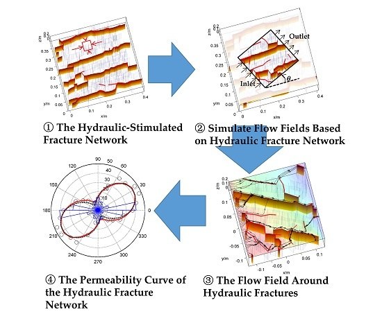
The investigation on the permeability of the fracture network provides an alternative way for quantifying the fracture network configuration during hydraulic stimulation. First, as hydraulic fracturing treatment is a fluid-rock coupling process, the investigation on the permeability of a small region is helpful in predicting the propagation behaviors of the hydraulic fracture network in a bigger region without knowing the propagation of each individual fracture in the bigger region. Second, as the aim of fracturing treatment is the permeability enhancement, the investigation of permeability is useful in answering how well the reservoir is stimulated. The structure of this paper is organized as follows. First, with a newly-developed numerical model based on DDM, the hydraulic fracturing processes are simulated based on the fracture network reconstructed from real shale samples. Then, the permeability of the hydraulic fracture network in different conditions is investigated to analyze the favorable conditions for the hydraulic fracturing treatment.

2. Numerical Method

2.1. Hydraulic Fracturing

A DDM-based model is used to simulate the propagation of the hydraulic fracture network. One of the advantages of DDM is the precise solving of the fracture aperture, which is required by the investigation of permeability, as fracture conductance is sensitively related to the fracture aperture. The details of the model have been introduced in our previous published papers [24,25,26]. For the sake of completeness, the model is briefly introduced below.

Given the normal and shear displacement discontinuities of each fracture element, the induced stresses by the opening and sliding of the fracture system with N elements can be calculated by [27]:

$$\begin{array}{l}{\mathsf{\sigma }}_n\left(x\right)={\displaystyle \sum _{r=1}^N{\displaystyle {\int }_0^{l_r}\left[G_{11}\left(x,s\right)w\left(s\right)+G_{12}\left(x,s\right)\mathsf{\nu }\left(s\right)\right]K\left(x,s\right)ds}}\\ {\mathsf{\tau }}_s\left(x\right)={\displaystyle \sum _{r=1}^N{\displaystyle {\int }_0^{l_r}\left[G_{21}\left(x,s\right)w\left(s\right)+G_{22}\left(x,s\right)\mathsf{\nu }\left(s\right)\right]K\left(x,s\right)ds}}\end{array}$$

(1)

where $x$ = (x, y) is the coordinate, w is the normal displacement discontinuity, ν is the shear displacement discontinuity, l_r is the length of fracture r, G_ij are the hyper singular Green’s functions, which are proportional to the plane strain Young’s modulus [27], σ_n is the normal stress and τ_s is the shear stress, obeying Coulomb’s frictional law characterized by the coefficient of friction λ, which limits the shear stress by:

$$\left|{\mathsf{\tau }}_s\right|\le \mathsf{\lambda }{\mathsf{\sigma }}_n$$

(2)

that can act in parts of fractures that are in contact, but vanishes along the separated parts. Along the opened fracture portions, we have:

$${\mathsf{\sigma }}_n=p_f$$

(3)

K is the three-dimensional correction coefficient. Using the parameters given by Wu and Olson [28], the correction coefficient K proposed by Olson [29] can be written as:

$$K\left(x_1,x_2\right)=1-\frac{d^3}{{\left[d^2-{\left(h/2\right)}^2\right]}^{3/2}}$$

(4)

where h is the limited layer thickness perpendicular to the simulation plain and d is the distance between points x₁ and x₂.

The fracture growth is based on the maximum hoop stress criterion, with the maximum mixed-mode intensity factor reaching a critical value:

$$\frac{1}{2}\cos \frac{{\theta }_0}{2}[K_I(1+\cos {\theta }_0-3K_{II}\sin {\theta }_0]=K_{IC}$$

(5)

where K_I and K_II are stress intensity factors, K_IC is the tensile mode fracture toughness and $\theta$ is the fracture propagation direction relative to the current fracture orientation and satisfies:

$$K_I\sin \theta +K_{II}(3\cos \theta -1)=0$$

(6)

Considering that the permeability of the shale matrix is ultra-low and shale gas transfer from the matrix to the fracture system in several years during production, while the water injection lasts only for hours during hydraulic fracturing treatment, the permeation depth of water into the shale matrix should be much smaller than the average spacing between the simulated fractures, which is generally at a scale of 0.1 m [30]. As a result, the fluid transfer and interaction between the fracture and the rock matrix is generally ignored during the modelling of hydraulic fracturing by many researchers [5,20,27,31,32].

As the aim of the modelling of fracture network propagation is the calculation of permeability, there is no need to simulate the propagation of the complex fracture network within the whole shale gas reservoir. By contrast, the configurations of the hydraulic-stimulated fracture network in a relatively smaller region is enough for the characterization of the permeability. In this work, the characterization of permeability is implemented based on the outcrop shale samples from the Longmaxi formation of China. The width of the shale samples is 0.4 m, which is much greater than the average spacing between natural fractures, and is much smaller than the scale of the shale gas reservoir. Therefore, the variation of fluid pressure within the simulation region could be neglected, i.e., the fluid viscosity is ignorable. The hydraulic fracturing process is simulated by increasing the fluid pressure in the fractures linked to the injection center step by step. Only the discretization of the fractures is needed during the solving. In this work, fractures are meshed with constant displacement discontinuity elements. When a fracture extends, new fracture elements are added to the tip of the fracture without the re-meshing of the existing grids.

2.2. Permeability Calculation

The permeability of the hydraulic-stimulated fracture network is calculated by simulating the single-phase incompressible flow under constant pressure difference at the two opposite sides of the fractured region. The single phase flow is simulated with a solver based on finite volume method. The hydraulically-fractured region is meshed with regular grids, and in each grid, the following equation exists:

$${\displaystyle \sum _j{g}_{ij}\left(p_i-p_j\right)}=0$$

(7)

for grid i and j. The conductivity g depends on the hydraulic fracture network configuration. For the two grids that are not linked by any fracture, g = k, where k is the permeability of rock matrix. For the two grids linked by a fracture, the conductivity g is calculated by:

$$g=k+\frac{w^3}{12\delta }\cdot \frac{L}{dx+dy}$$

(8)

where $\delta$ is the grid width, w is the fracture aperture, L is the length of the fracture segment and dx and dy are the distances between the two ends of the fractures along x and y axis directions, respectively.

3. Model Validation

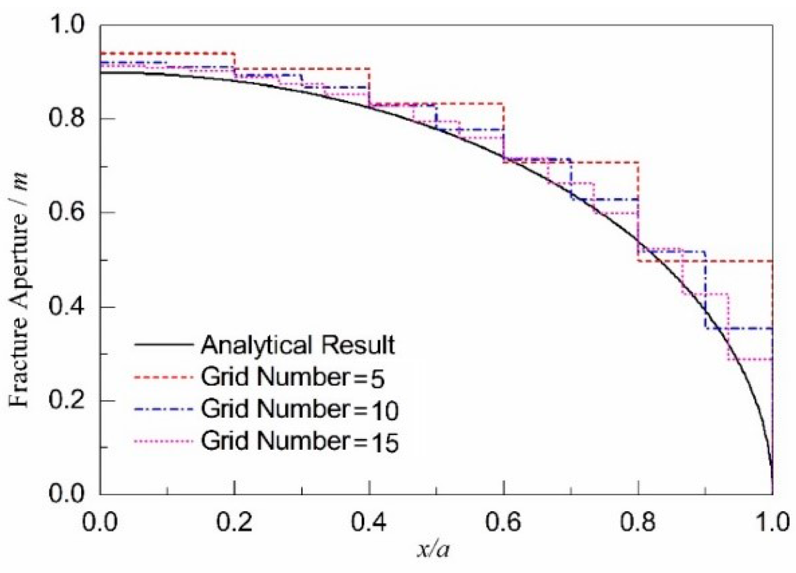
The calculation of the fracture aperture is one of the most important foundations of the model. Given the fluid pressure, the aperture profile of a single fracture in infinite rock follows [33]:

$$w\left(x\right)=-\frac{2\left(1-{\nu }_{Po}\right)}{G}{p}_{f}a\sqrt{1-\frac{x^2}{a^2}}$$

(9)

where w is the fracture aperture, a is the fracture half length, p_f is the net fluid pressure, x is the distance to the center of the fracture, G is the shear modulus and ν_Po is Poisson’s ratio.

The numerical model is validated against the analytical solution. A single fracture is simulated with the parameters listed in

Table 1. Input parameters for the calculation of the fracture aperture, where p_f is fluid pressure, G is shear modulus and ${\mathsf{\sigma }}_x$ and ${\mathsf{\sigma }}_y$ are the principle stresses along the x and y axis directions, respectively.

Parameter	Value	Parameter	Value
Fracture Length	1 m	Layer Thickness	Infinite
$p_f/G$	1	Far-Field Stress	${\mathsf{\sigma }}_x={\mathsf{\sigma }}_y=0$
Poisson’s Ratio	0.1

. The aperture is compared with the analytical solution, as shown in Figure 1. The numerical results agree well with the analytical one, even when there are only five grids.

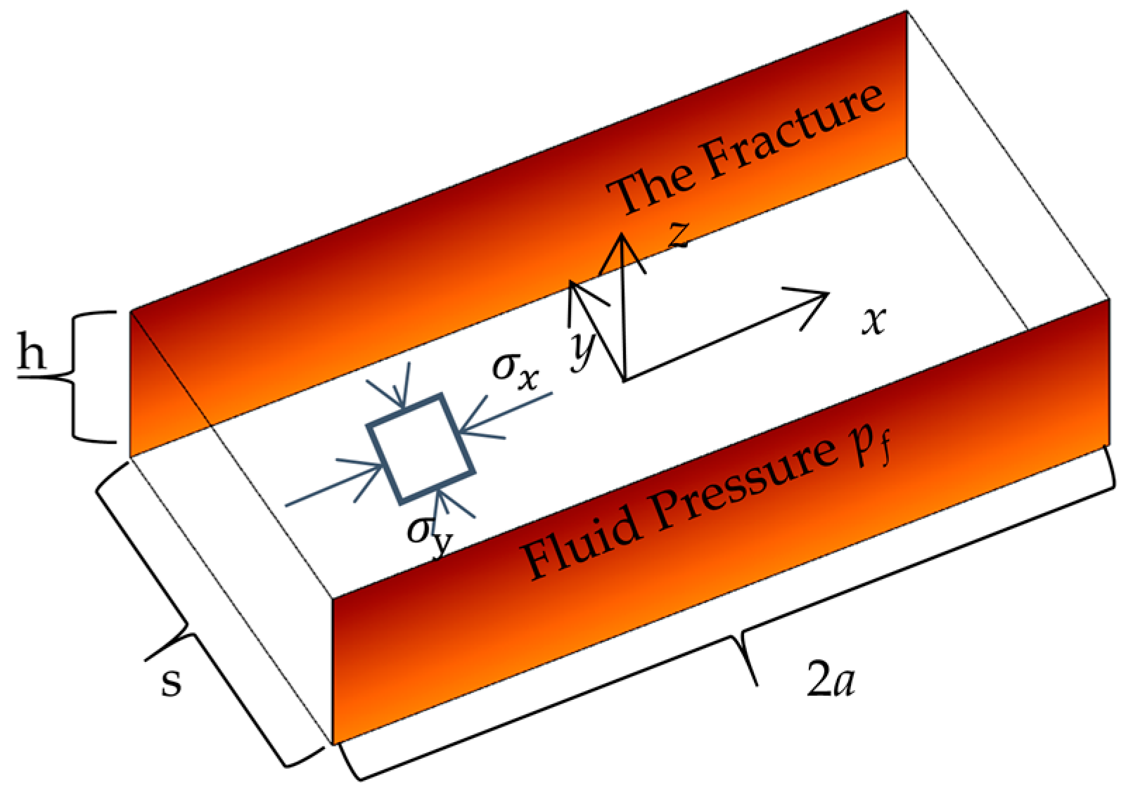
The stress interactions between different fractures are important for the propagation of the fracture network. In this work, the stress field around two parallel fractures is calculated, and the stress field is compared with Fast Lagrangian Analysis of Continua (FLAC) 3D and Kresse et al. [31]. It must be noted that, due to the stress interactions between the two fractures, the aperture of these two fractures is different with the aperture of a single fracture, as given by Equation (9). The stress field around the two parallel fractures can be correctly calculated only when the stress interactions between them are correctly simulated. The numerical setting is shown in Figure 2 Constant internal fluid pressure is applied to the two fractures. For these two fractures, s/h = 0.5 and h/a = 0.3, where s is the spacing between these two fractures, h is the fracture height and a is the fracture half length. 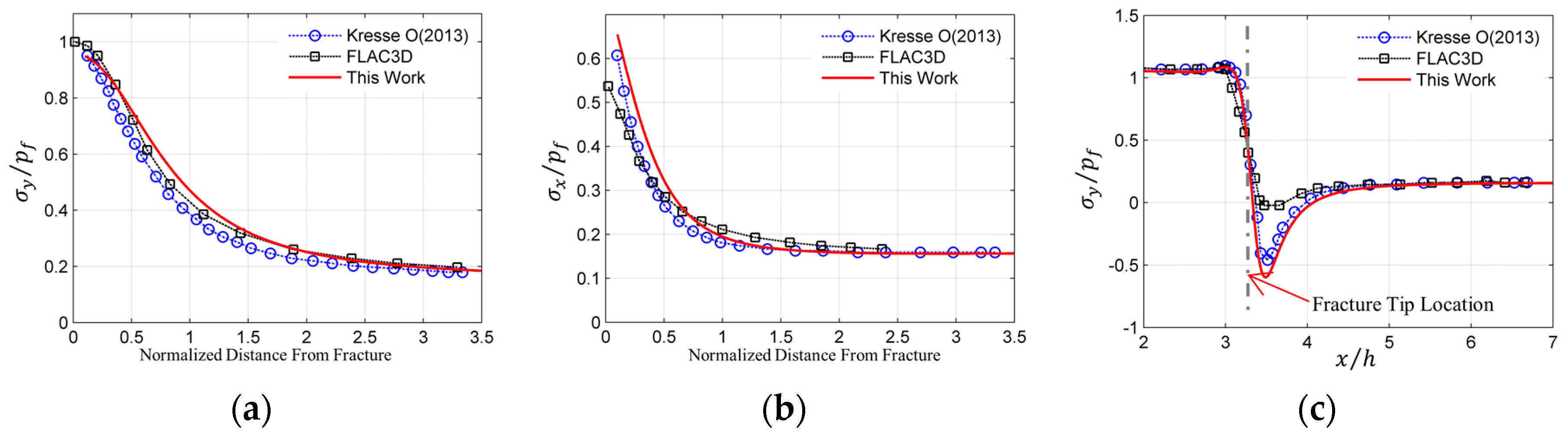The origin of the coordinate system as shown in Figure 2 is at the center of the two fractures. The stresses along the x axis (y = 0, z = 0 and x > 0) and y axis (x = 0, z = 0 and y > s/2) are compared. The results are shown in Figure 3. The numerical results of this work match closely with the former works.

4. Results and Discussion

4.1. Hydraulic Fracture Network

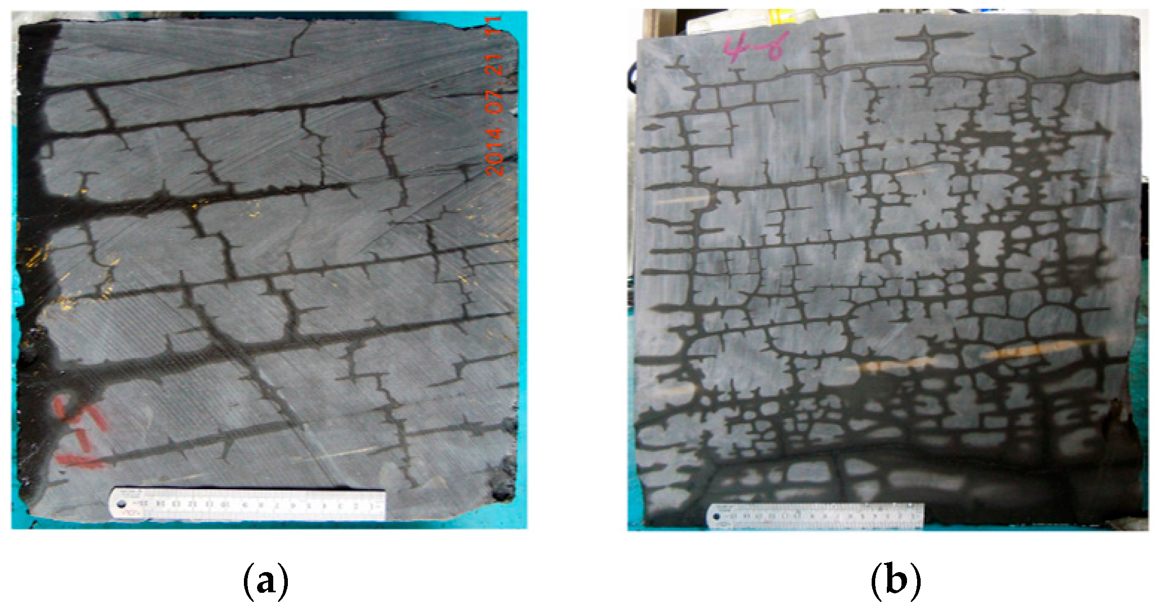
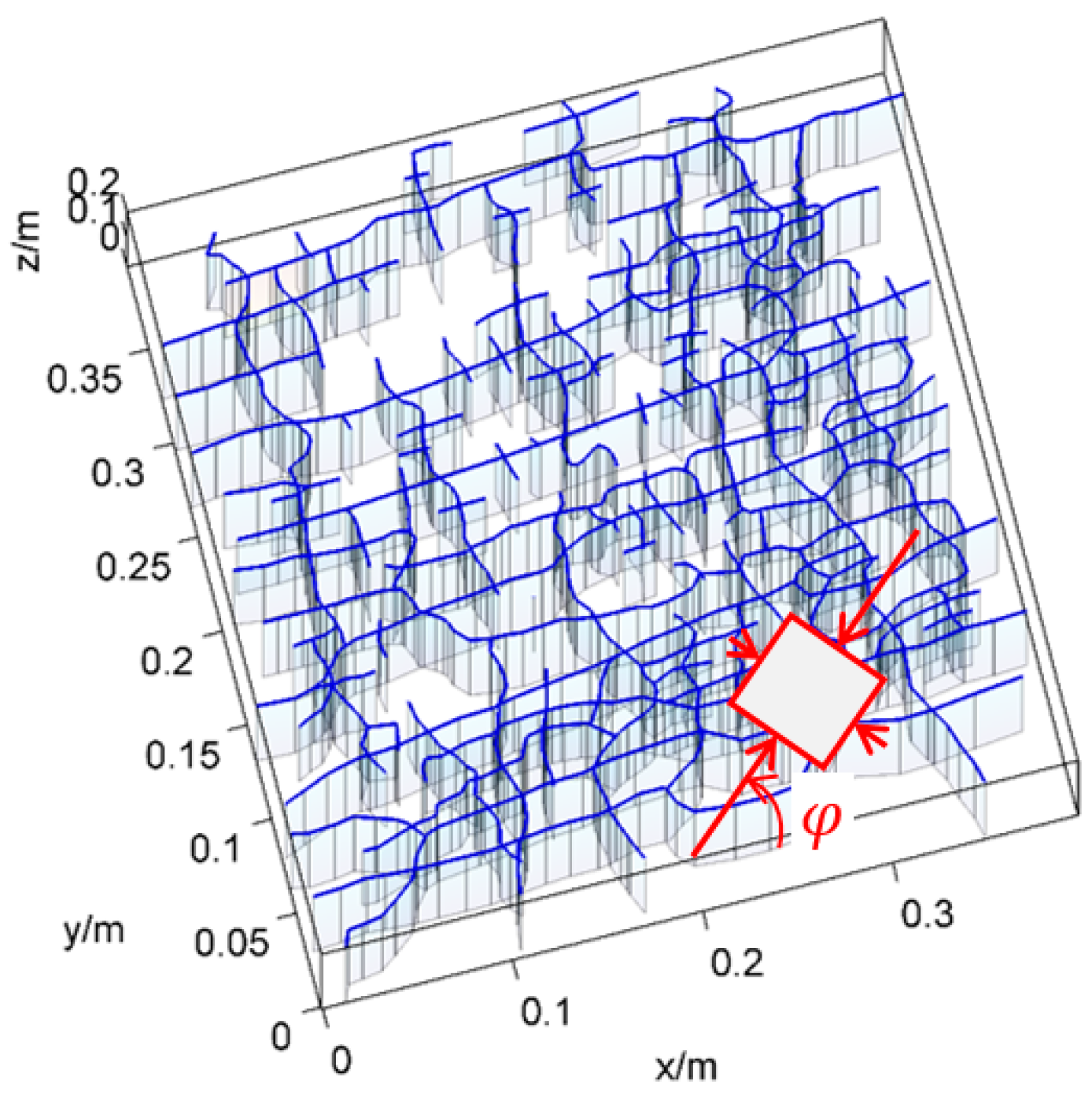
The fracture propagation processes are simulated based on the fracture networks reconstructed from the shale samples from the Longmaxi formation of China, as shown in Figure 4. The natural fracture networks are well developed and can be roughly divided into two sets. The length is longer and the conductivity is better for the horizontal set of fractures. The numerical setting is shown in Figure 5. All p_f the natural fractures are initially closed with the fluid pressure equaling zero. A constant far field stress condition is applied to the model during the modelling. The maximum principle stress direction is represented by the angle $\phi$, as shown in Figure 5. The width of the simulation region is 0.4 m, which is much smaller than the scale of shale gas reservoirs. Therefore, the variation of fluid pressure within the region could be neglected, i.e., the fluid viscosity is ignorable. Moreover, as the natural fractures are well developed, fluid enters all of the connected fractures once fluid reaches the boundary of the region.

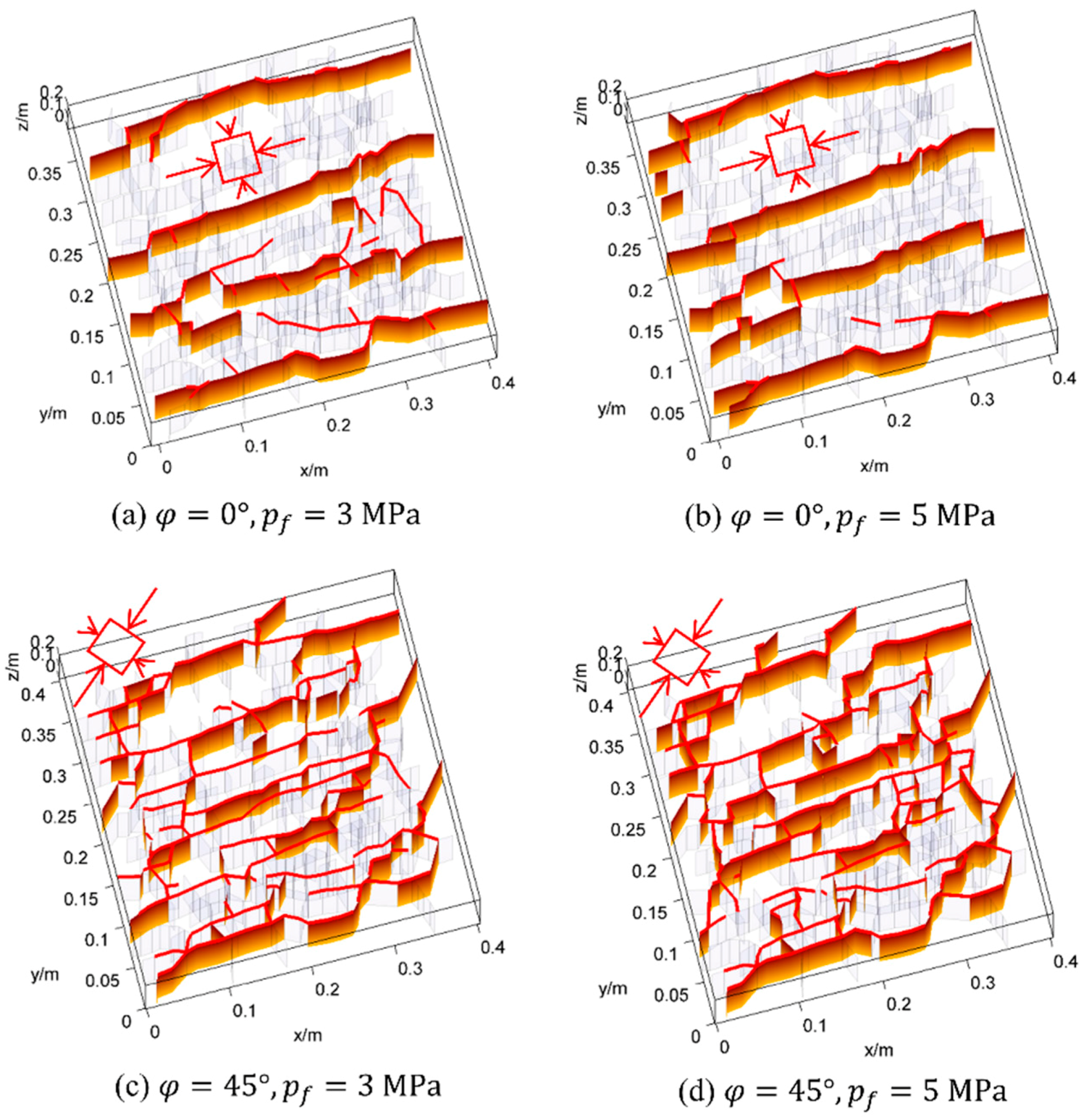
Hydraulic fracturing processes are simulated with the parameters listed in

Table 2. Input parameters for modelling the hydraulic fracturing process.

Parameter	Value	Parameter	Value
Stress Difference	4 MPa	Layer Thickness	0.2 m
Fracture Toughness	1.0 MPa·m0.5	Young’s Modulus	1.8 × 1010 Pa
Poisson’s Ratio	0.1	The Friction Coefficient	0.9

. The simulations are implemented by increasing the fluid pressure step by step. The fracture networks under different stress directions and fluid net pressures are shown in Figure 6. As the natural fracture network is well developed, the initiation of new fractures and the propagation of hydraulic fractures are ignorable. The fracture networks after fluid injection depend on both the crustal stress condition and the natural fractures. The reopening of natural fractures is mainly along the maximum principle stress direction. Moreover, although fluid net pressure has great effects on the fracture aperture, it has ignorable effects on the configuration of the reopened natural fracture. In short, the main natural fractures and the crustal stress condition are the key parameters in determining the hydraulic fracture network configuration.

4.2. Flow Fields in the Fracture System

Flow fields are simulated to calculate the permeability of the fracture network. The numerical setting is illustrated in Figure 7. All of the fracture details, including the fracture apertures and fracture locations, are obtained from the results of hydraulic fracturing simulations. The sub-regions of the fracturing region are used. The width of the sub-region is 0.25 m. The orientation of the sub-region is quantified by the angle $\theta$, as in Figure 7. The fluid flow outside the sub-region is ignored. The flow fields in the sub-region are simulated by applying a constant pressure difference at the two opposite sides of the sub-regions.

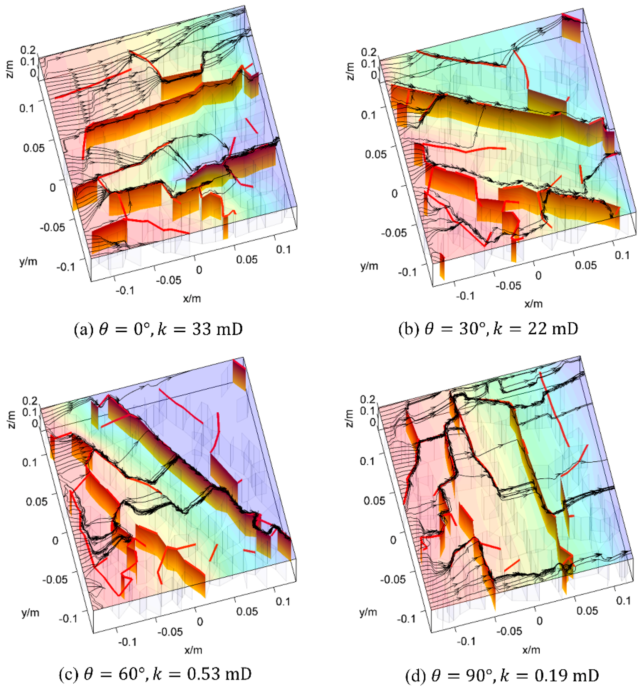
The flow fields in the sub-regions are shown in Figure 8. The reopened natural fractures are the main flow paths and have great effects on the flow fields. Most of the streamlines that are starting uniformly from the inlets, as shown in Figure 8, converge into the reopened natural fractures. The flow field also varies significantly with the orientation of the sub-region. When $\theta =0°$, i.e., the flow direction is approximately parallel to the main natural fractures, the flow path is shorter, and the permeability is stronger. By contrast, when $\theta$ is bigger, the flow path is longer and narrower; thus, the permeability is poorer. In short, the flow fields are much different for the sub-regions under different orientations.

4.3. Effects of Fluid Pressure

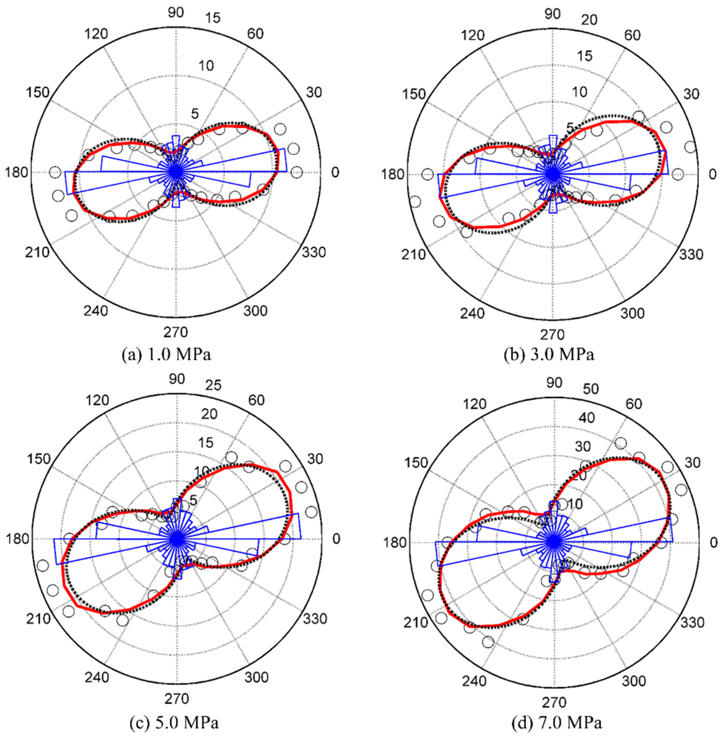
The permeability of the fracture network is calculated by simulating the flow fields in the sub-regions under different orientations. The occurrence of the reopened natural fractures and the permeability under different directions are shown in Figure 9. Fluid pressure has ignorable effects on the occurrences of the reopened fractures, which is consistent with the observations in Section 4.1. The permeability increases significantly with the increasing of fluid net pressure, which is caused by the bigger fracture aperture under higher fluid net pressure. Moreover, the permeability anisotropy is very strong, as shown in the figures. When fluid net pressure is low, as in Figure 9a,b, the fracture network permeability is dominated by the main natural fracture direction, which is approximately parallel to the x axis direction. By contrast, when the fluid pressure is high, as shown in Figure 9c,d, the fracture network permeability is controlled by the directions of both crustal stress and the main natural fractures.

These permeability curves shown in Figure 9 have similar shapes. With the variation of the view angle $\theta$, the permeability of the fracture network varies gradually between the maximum and the minimum values. For the convenient use of the permeability curves, a fitting formula of permeability is given as follows,

$$k(\theta )=\frac{k_{\max }+k_{\min }}{2}+\frac{k_{\max }-k_{\min }}{2}\sin (\theta -{\theta }_{\max }+\frac{\mathsf{\pi }}{4})$$

(10)

where k_min and k_max are the minimum and maximum values of permeability, respectively, and ${\theta }_{\max }$ is the angle when the maximum permeability is reached. Given these three fitting parameters, the permeability of the hydraulic fracture network can be well described by Equation (10). For the permeability curves shown in Figure 9, the fitting parameters are listed in

Table 3. The fitting parameters for the permeability curves under different fluid net pressures. Here, p_f is fluid net pressure.

pf/MPa	${\mathit{\theta }}_{\mathbf{max}}$	kmin/mD	kmax/mD
1.0	8.6$°$	1.0	10.5
3.0	13.8$°$	1.5	15.0
5.0	22.9$°$	4.0	20.0
7.0	28.1$°$	7.0	43.0

. It can be seen that the fitting curves agree well with the smoothed data.

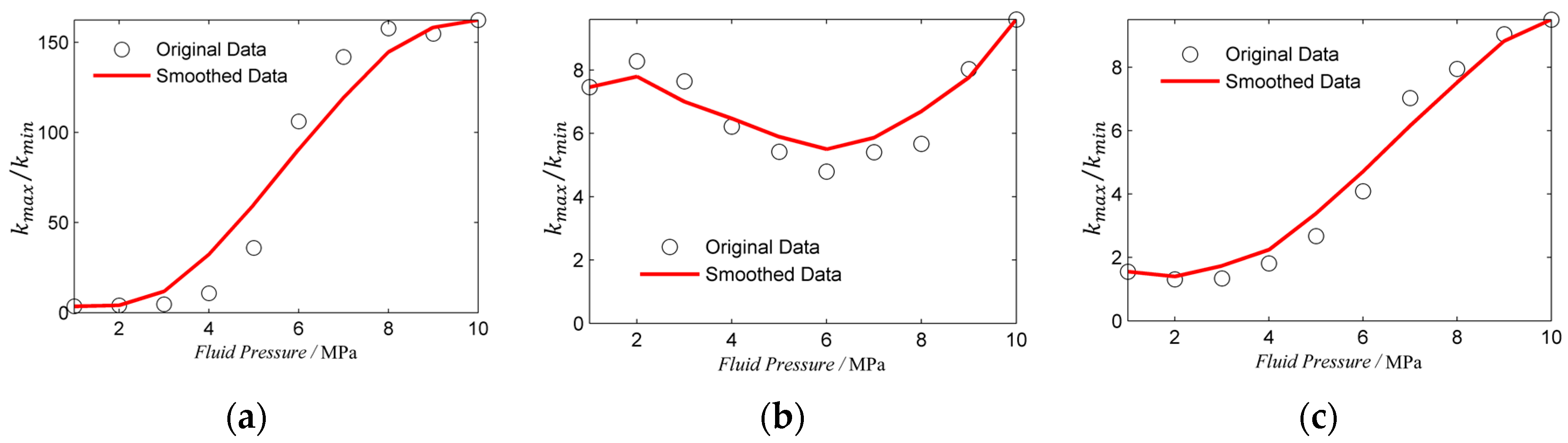
The permeability anisotropy is unfavorable to the hydraulic fracturing treatment. The flow resistant varies more significantly with direction, and thus, the main hydraulic fractures are more easily formed when the permeability anisotropy is stronger. For convenience, we define the permeability anisotropy as k_max/k_min. The variations of the permeability anisotropy with fluid net pressure under different crustal directions are shown in Figure 10. By comparing the results in Figure 10, it is found that the permeability anisotropy is weaker when $\phi =45°$ and $\phi =90°$, i.e., the complex fracture network is more easily to formed when the angle $\phi$ is bigger. Moreover, when the intersection angle between the maximum principle stress direction and the natural fracture direction is small, as in Figure 10a,c, the permeability anisotropy increases with fluid net pressure. This is caused by the fact that most of the fractures are tensile fractures when the maximum principle stress direction is parallel to the natural fracture direction, and the increasing of the fractures aperture with fluid net pressure is more significant along the maximum principle stress direction. When the intersection angle $\phi =45°$, as in Figure 10b, the permeability anisotropy first decreases when the fluid net pressure is smaller than 6 MPa and then increases with fluid net pressure when the fluid net pressure is bigger. The decreasing of the permeability anisotropy when the fluid net pressure is smaller than 6 MPa is caused by the formation of the shear fracture network. With the increasing of fluid net pressure, the shear fracture network is first formed. As the conductance of a shear fracture is mainly related to the roughness of the fracture surface, the permeability anisotropy is much weaker for the shear fracture network. Therefore, the formation of the shear fracture network is favorable to the evolution of the hydraulic fracture network afterwards.

4.4. Effects of Stress Direction

The stress direction is one of the most important parameters to quantify the anisotropy of shale gas reservoirs. We simulated the hydraulic fracturing process under different stress directions. The results are shown in Figure 11. The corresponding fitting parameters for the fitting curves are listed in

Table 4. The fitting parameters for the permeability curves under different stress directions.

$\mathit{\phi }$	${\mathit{\theta }}_{\mathbf{max}}$	kmin/mD	kmax/mD
$0°$	2.9$°$	0.4	2.1
$30°$	11.5$°$	0.4	4.0
$45°$	29.8$°$	0.5	5.5
$90°$	101.4$°$	0.8	1.1

. The stress direction has great effects on the occurrence of the fractures reopened by fluid pressure under different directions. The natural fractures with a small intersection angle with the maximum principle stress direction tend to be reopened during the hydraulic fracturing process. However, as there are only two orthogonal sets of natural fractures, the occurrence of the reopened fractures does not reach the maximum value along the maximum principle stress direction. The stress direction has great effects on the permeability. The permeability reaches the maximum value between the directions of the maximum principle stress and the main natural fractures. For example, the maximum permeability is reached when the angle $\theta$ approximately equals $15°$ and $30°$, respectively, when the angle of maximum principle stress equals $30°$ and $60°$, respectively, as shown in Figure 11b,c. Moreover, the permeability is bigger when the maximum principle stress direction is neither parallel to nor perpendicular to the main natural fracture direction, as shown in Figure 11b,c. This is caused by the formation of the shear fracture network.

The variations of permeability anisotropy with stress direction are shown in Figure 12. First, when the angle $\phi$ increases from $0°$ to $45°$, the variation of permeability anisotropy depends on fluid net pressure. This can be explained by the formation of the shear fracture network. The fluid net pressure has great effects on the aperture of fractures, but has ignorable effects on the shearing of fractures. When $\phi =0°$, the permeability is influenced only by tensile fractures. By contrast, when $\phi =45°$, the permeability is created by both the tensile mode and the shear mode fractures. As the permeability anisotropy increases dramatically with fluid pressure when $\phi =0°$, as shown in Figure 10a, the permeability anisotropy increases when fluid net pressure is lower and decreases when fluid net pressure is higher when the angle $\phi$ increases from $0°$ to $45°$. Second, when the angle $\phi$ increases from $45°$ to $90°$, the permeability anisotropy decreases. The weaker permeability anisotropy when $\phi =90°$ is caused by the increasing of permeability perpendicular to the main natural fracture direction.

5. Conclusions

In this paper, the permeability of the hydraulically-stimulated fracture network in shale gas reservoirs is investigated by a numerical model based on the displacement discontinuity method. The hydraulic fracturing processes under different fluid net pressures and crustal stress conditions are simulated based on the natural fracture network reconstructed from the Longmaxi formation of China. The fracture network permeability is then investigated based on the fracture configurations obtained from the hydraulic fracturing simulations.

Firstly, the hydraulic fracturing processes and the flow field in different directions are simulated. As the natural fracture network is well developed, the increasing of the fracture network permeability is caused mainly by the reopening of the pre-existing natural fractures, not the propagation of hydraulic fractures. The configuration of the hydraulic fracture network is affected greatly by the crustal stress condition. The fluid net pressure also has great effects on the fracturing process and the fracture aperture, but has ignorable effects on the fracture network configurations. Both the stress direction and the fluid net pressure have great effects on the permeability of the hydraulic fracture network.

Secondly, the effects of fluid net pressure are investigated. The permeability anisotropy is stronger when the fluid pressure is higher. The strong permeability anisotropy is unfavorable to the formation of the complex fracture network. When fluid net pressure is low, the permeability is controlled by the natural fractures, and the maximum permeability is reached along the main natural fracture direction. By contrast, when fluid net pressure is high, the permeability is controlled by both the natural fracture and the crustal stress condition, and the maximum permeability is reached between the maximum principle stress direction and the main natural fracture direction.

Thirdly, the effects of crustal stress direction are investigated. The crustal stress direction has great effects on the permeability anisotropy of the hydraulic fracture network. The permeability anisotropy reaches the minimum value when the maximum principle stress direction is perpendicular to the main natural fracture direction. The weaker permeability anisotropy can suppress the formation of the main hydraulic fractures and, thus, is favorable to the formation of the complex fracture network.

Finally, as the permeability curves under different conditions have similar shapes, a fitting equation, which contains three fitting parameters, is given. By using the proper values of the fitting parameters, the fitting curves agree well with the smoothed curves of the permeability. The fitting equation is useful for the further usage of the permeability curves.

References

- Meng, Q.M.; Zhang, S.C.; Guo, X.M.; Chen, X.H.; Zhang, Y. A primary investigation on propagation mechanism for hydraulic fracture in glutenite formation. J. Oil Gas Technol. 2010, 32, 119–123. [Google Scholar]
- Bunger, A.P.; Gordeliy, E.; Detournay, E. Comparison between laboratory experiments and coupled simulations of saucer-shaped hydraulic fractures in homogeneous brittle-elastic solids. J. Mech. Phys. Solids 2013, 61, 1636–1654. [Google Scholar] [CrossRef]
- Huang, H.; Zhang, F.; Callahan, P.; Ayoub, J.A. Fluid injection experiments in 2d porous media. SPE J. 2012, 17, 903–911. [Google Scholar] [CrossRef]
- McClure, M.; Horne, R. Characterizing hydraulic fracturing with a tendency-for-shear-stimulation test. SPE Reserv. Eval. Eng. 2014, 17, 233–243. [Google Scholar] [CrossRef]
- Wu, K.; Olson, J.E. Simultaneous multifracture treatments: Fully coupled fluid flow and fracture mechanics for horizontal wells. SPE J. 2014, 20, 337–346. [Google Scholar] [CrossRef]
- Perkins, T.K.; Kern, L.R. Widths of hydraulic fractures. J. Petrol. Technol. 1961, 13, 937–949. [Google Scholar] [CrossRef]
- Nordgren, R.P. Propagation of a vertical hydraulic fracture. Soc. Petrol. Eng. J. 1972, 12, 306–314. [Google Scholar] [CrossRef]
- Geertsma, J.; De Klerk, F. Rapid method of predicting width and extent of hydraulically induced fractures. J. Petrol. Technol. 1969, 21, 1571–1581. [Google Scholar] [CrossRef]
- Advani, S.H.; Lee, T.S.; Lee, J.K. Three-dimensional modeling of hydraulic fractures in layered media: Part I—Finite element formulations. J. Energy Resour. Technol. 1990, 112, 1–9. [Google Scholar] [CrossRef]
- Siebrits, E.; Peirce, A.P. An efficient multi-layer planar 3d fracture growth algorithm using a fixed mesh approach. Int. J. Numer. Meth. Eng. 2002, 53, 691–717. [Google Scholar] [CrossRef]
- Li, H.; Liu, C.L.; Mizuta, Y.; Kayupov, M.A. Crack edge element of three-dimensional displacement discontinuity method with boundary division into triangular leaf elements. Commun. Numer. Meth. Eng. 2001, 17, 365–378. [Google Scholar] [CrossRef]
- Yan, X.Q.; Liu, B.L. Fatigue growth modeling of cracks emanating from a circular hole in infinite plate. Meccanica 2012, 47, 221–233. [Google Scholar] [CrossRef]
- Birgisson, B.; Wang, J.L.; Roque, R.; Sangpetngam, B. Numerical implementation of a strain energy-based fracture model for HMA materials. Road Mater. Pavement Des. 2007, 8, 7–45. [Google Scholar] [CrossRef]
- Dong, C.Y.; Lo, S.H.; Cheung, Y.K. Numerical analysis of the inclusion-crack interactions using an integral equation. Comput. Mech. 2003, 30, 119–130. [Google Scholar] [CrossRef]
- Nagel, N.B.; Sanchez-Nagel, M. Stress shadowing and microseismic events: A numerical evaluation. In Proceeding of The SPE Annual Technical Conference and Exhibition, Denver, CO, USA, 30 October–2 November 2011.
- Rahman, M.M.; Rahman, S.S. Studies of hydraulic fracture-propagation behavior in presence of natural fractures: Fully coupled fractured-reservoir modeling in poroelastic environments. Int. J. Geomech. 2013, 13, 809–826. [Google Scholar] [CrossRef]
- Liu, F.S.; Borja, R.I. Extended finite element framework for fault rupture dynamics including bulk plasticity. Inter. J. Numer. Anal. Met. 2013, 37, 3087–3111. [Google Scholar] [CrossRef]
- Mohammadnejad, T.; Khoei, A.R. An extended finite element method for fluid flow in partially saturated porous media with weak discontinuities; the convergence analysis of local enrichment strategies. Comput. Mech. 2013, 51, 327–345. [Google Scholar] [CrossRef]
- Gordeliy, E.; Peirce, A. Coupling schemes for modeling hydraulic fracture propagation using the XFEM. Comput. Methods Appl. Mech. Eng. 2013, 253, 305–322. [Google Scholar] [CrossRef]
- Fu, P.C.; Johnson, S.M.; Carrigan, C.R. An explicitly coupled hydro-geomechanical model for simulating hydraulic fracturing in arbitrary discrete fracture networks. Inter. J. Numer. Anal. Methods Geomech. 2013, 37, 2278–2300. [Google Scholar] [CrossRef]
- Riahi, A.; Damjanac, B. Numerical study of interaction between hydraulic fracture and discrete fracture network. In Proceedings of the ISRM International Conference for Effective and Sustainable Hydraulic Fracturing, Brisbane, Australia, 20–22 May 2013.
- Rabczuk, T.; Belytschko, T. A three-dimensional large deformation meshfree method for arbitrary evolving cracks. Comput. Methods Appl. Mech. Eng. 2007, 196, 2777–2799. [Google Scholar] [CrossRef]
- Rabczuk, T.; Belytschko, T. Cracking particles: A simplified meshfree method for arbitrary evolving cracks. Int. J. Numer. Meth. Eng. 2004, 61, 2316–2343. [Google Scholar] [CrossRef]
- Zhang, Z.; Li, X. Numerical study on the formation of shear fracture network. Energies 2016, 9, 299. [Google Scholar] [CrossRef]
- Zhang, Z.; Li, X.; Yuan, W.; He, J.; Li, G.; Wu, Y. Numerical analysis on the optimization of hydraulic fracture networks. Energies 2015, 8, 12061–12079. [Google Scholar] [CrossRef]
- Zhang, Z.; Li, X.; He, J.; Wu, Y.; Zhang, B. Numerical analysis on the stability of hydraulic fracture propagation. Energies 2015, 8, 9860–9877. [Google Scholar] [CrossRef]
- Zhang, X.; Jeffrey, R. Development of fracture networks through hydraulic fracture growth in naturally fractured reservoirs. In Proceedings of the ISRM International Conference for Effective and Sustainable Hydraulic Fracturing, Brisbane, Australia, 20–22 May 2013.
- Wu, K.; Olson, J.E. Investigation of the impact of fracture spacing and fluid properties for interfering simultaneously or sequentially generated hydraulic fractures. SPE Prod. Oper. 2013, 28, 427–436. [Google Scholar] [CrossRef]
- Olson, J.E. Predicting fracture swarms—The influence of subcritical crackgrowth and the crack-tip process zone on joint spacing in rock. In The Initiation, Propagation, and Arrest of Joints and Other Fractures; Geological Society of London Special Publication: London, UK, 2004; pp. 73–87. [Google Scholar]
- Bazant, Z.P.; Salviato, M.; Chau, V.T.; Viswanathan, H.; Zubelewicz, A. Why fracking works. J. Appl. Mech. 2014, 81. [Google Scholar] [CrossRef]
- Kresse, O.; Weng, X.W.; Gu, H.R.; Wu, R.T. Numerical modeling of hydraulic fractures interaction in complex naturally fractured formations. Rock Mech. Rock Eng. 2013, 46, 555–568. [Google Scholar] [CrossRef]
- Weng, X.W. Modeling of complex hydraulic fractures in naturally fractured formation. J. Unconv. Oil Gas Res. 2015, 9, 114–135. [Google Scholar] [CrossRef]
- Crouch, S.L.; Starfield, A.M. Boundary Element Methods in Solid Mechanics; George Allen & Unwin: London, UK, 1983. [Google Scholar]
© 2016 by the authors; licensee MDPI, Basel, Switzerland. This article is an open access article distributed under the terms and conditions of the Creative Commons Attribution (CC-BY) license (http://creativecommons.org/licenses/by/4.0/).