
Impacts of Salinity on Saint-Augustin Lake, Canada: Remediation Measures at Watershed Scale

Abstract
: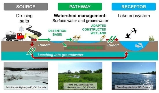
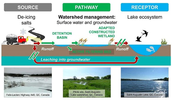
1. Introduction
2. Materials and Methods
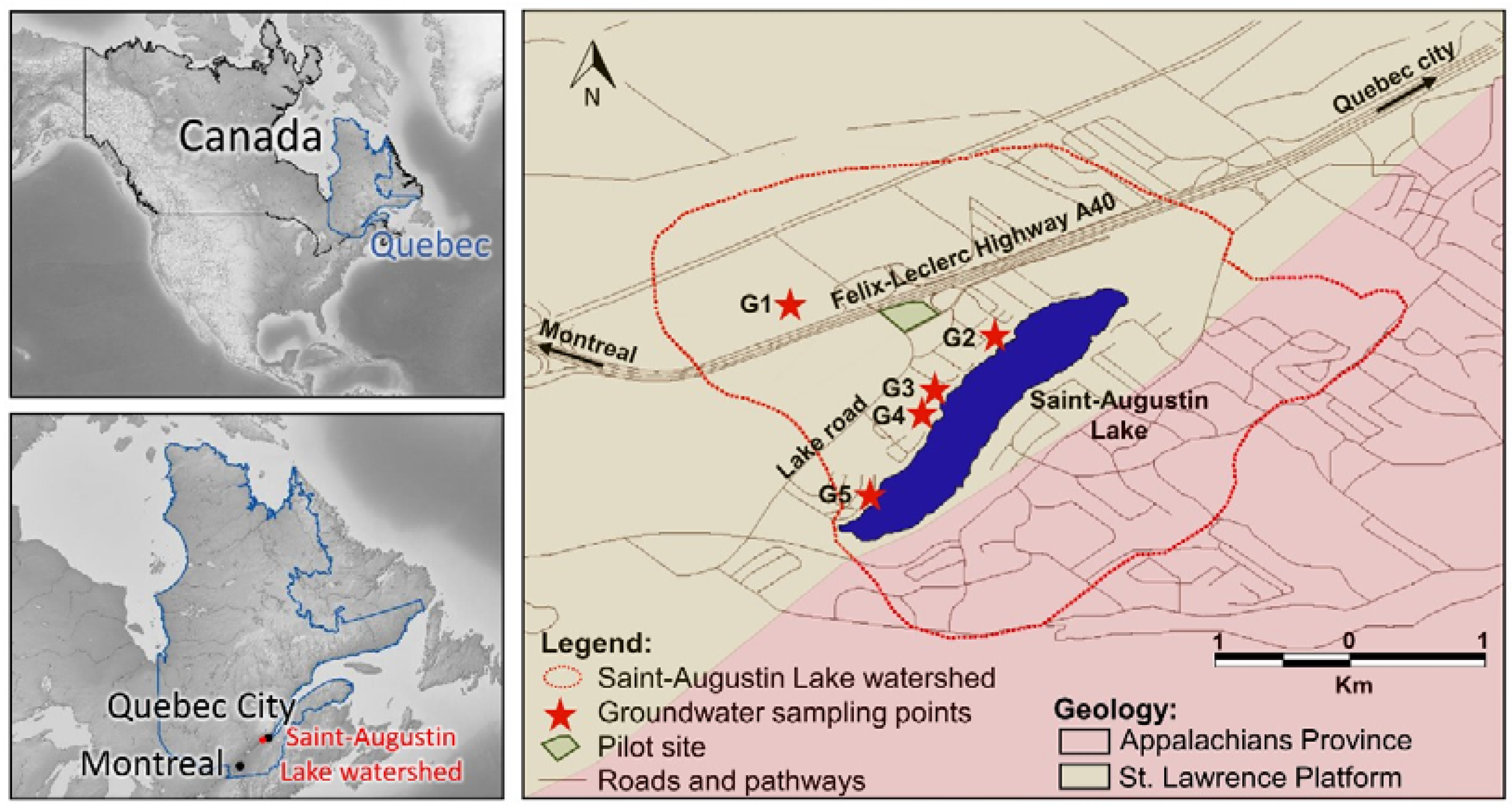
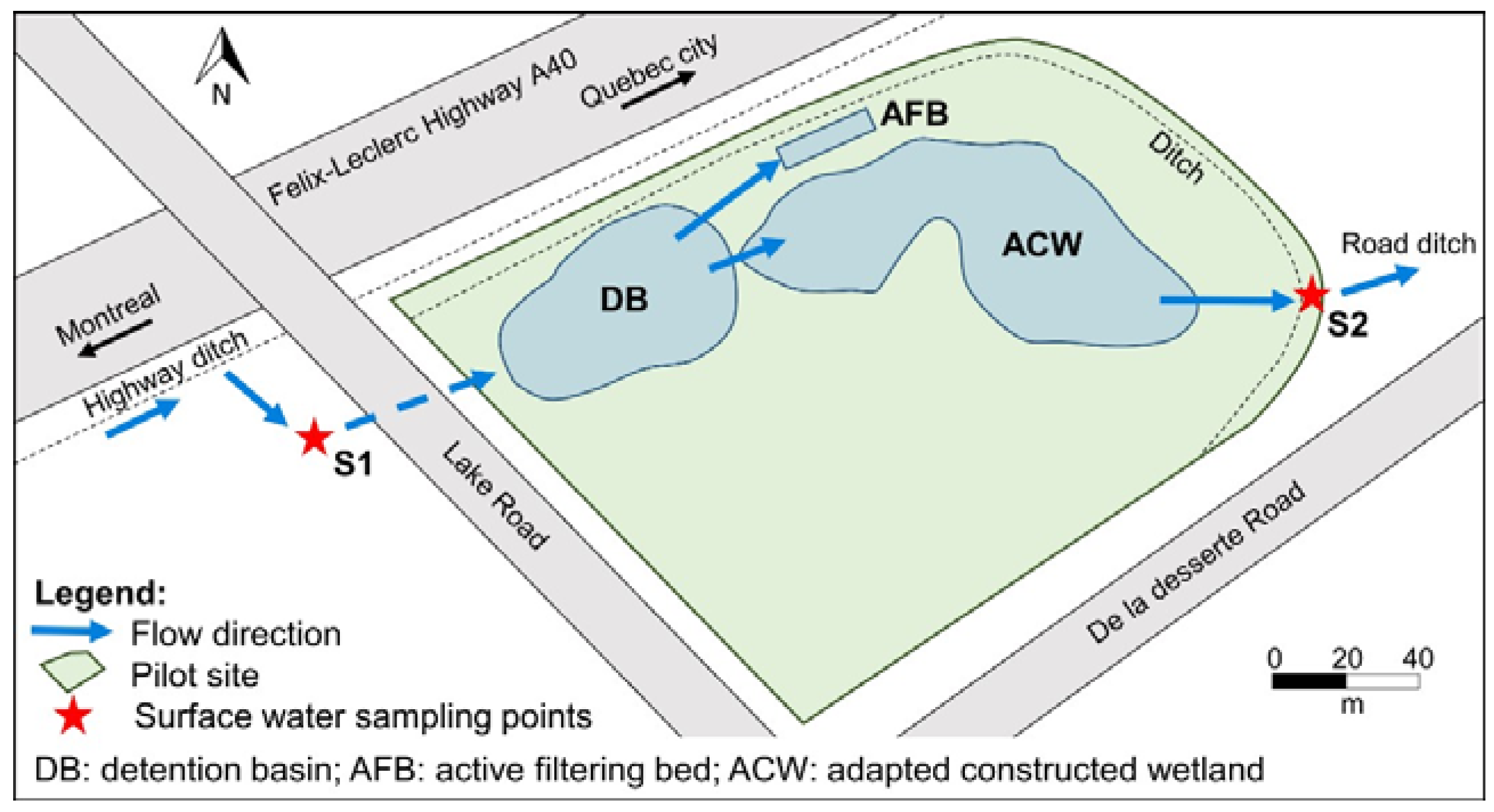
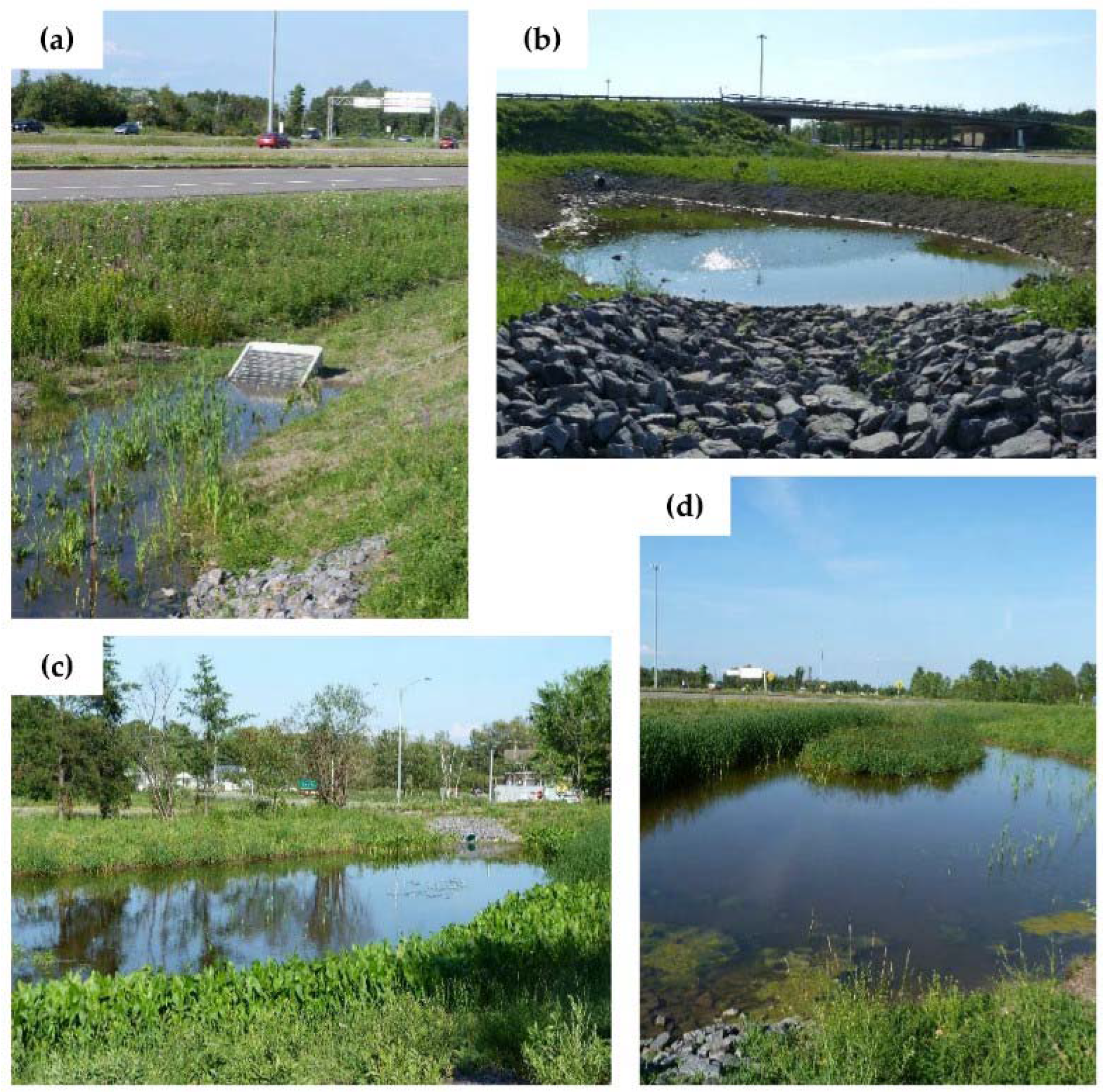
2.1. Site Description
2.2. Pilot Site Characteristic
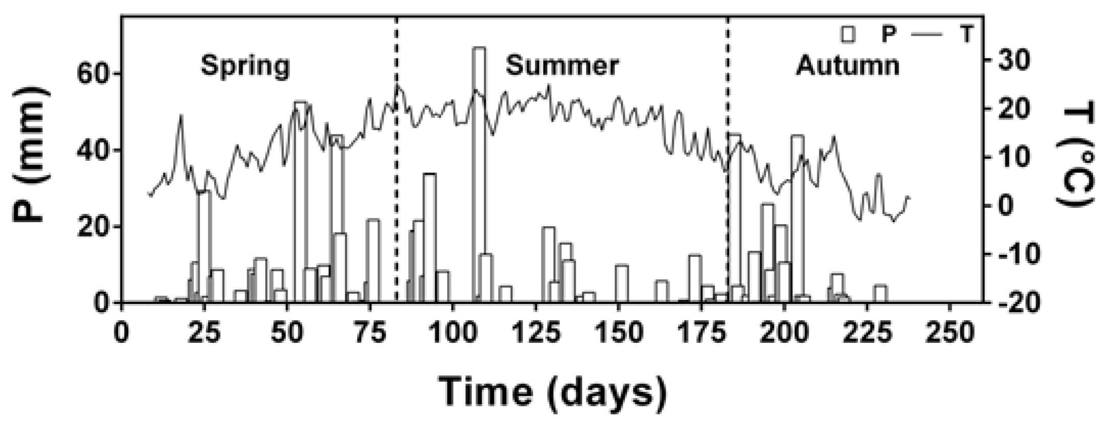
2.3. Sampling Strategy
2.3.1. Groundwater
2.3.2. Surface Water
2.4. Analytical Methods
2.5. Statistical Analyses
3. Results and Discussion
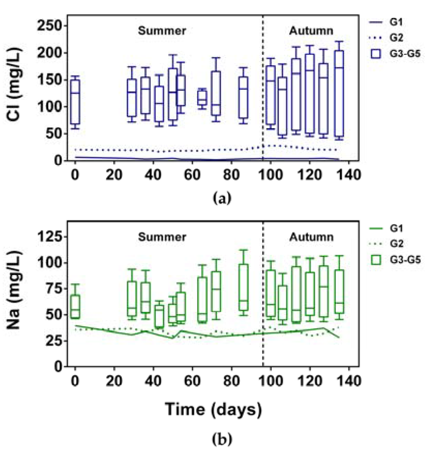
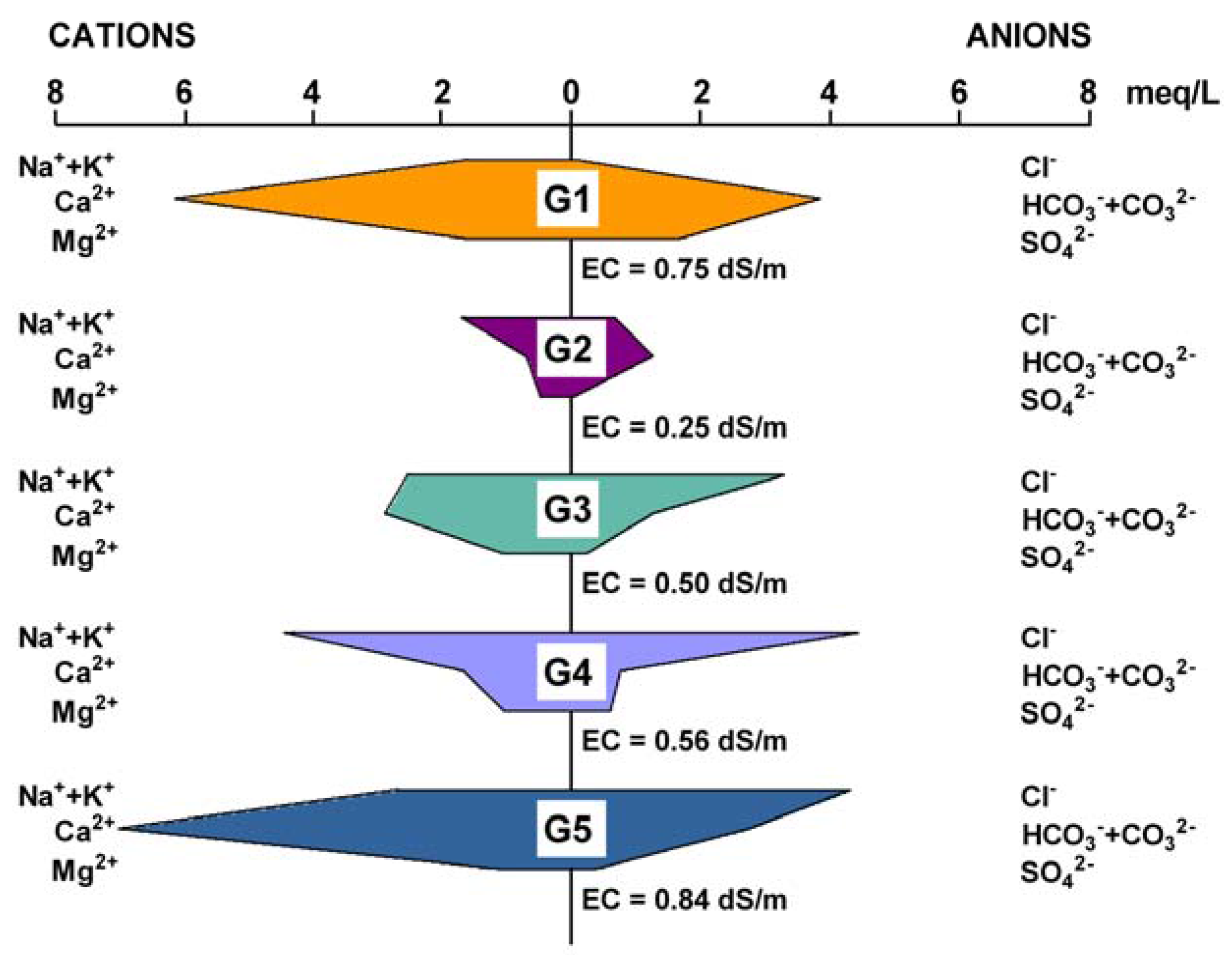
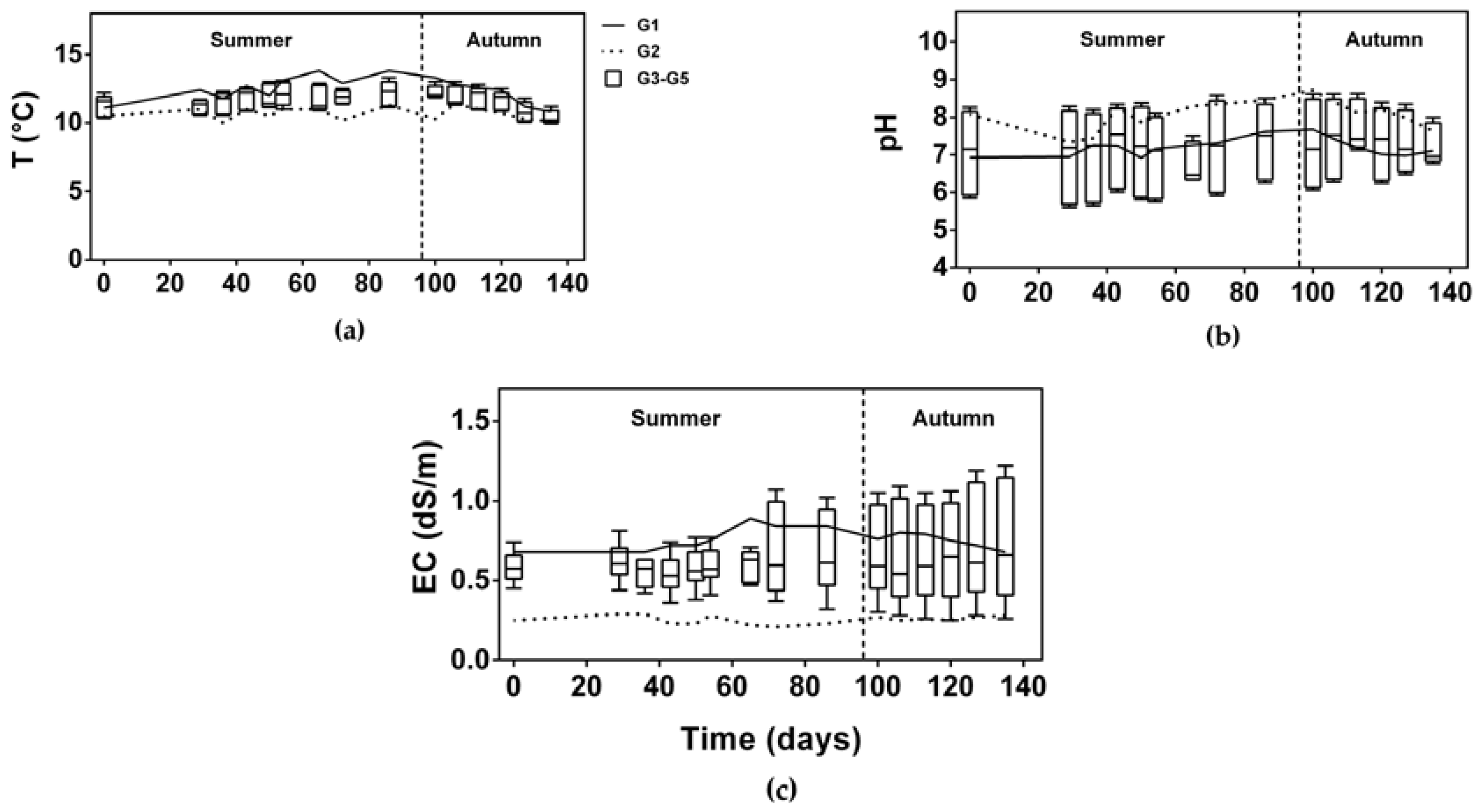
3.1. Groundwater Quality
3.1.1. Hydrochemical Groundwater Characterization
3.1.2. Water Quality Indicators
3.1.3. NaCl Concentration
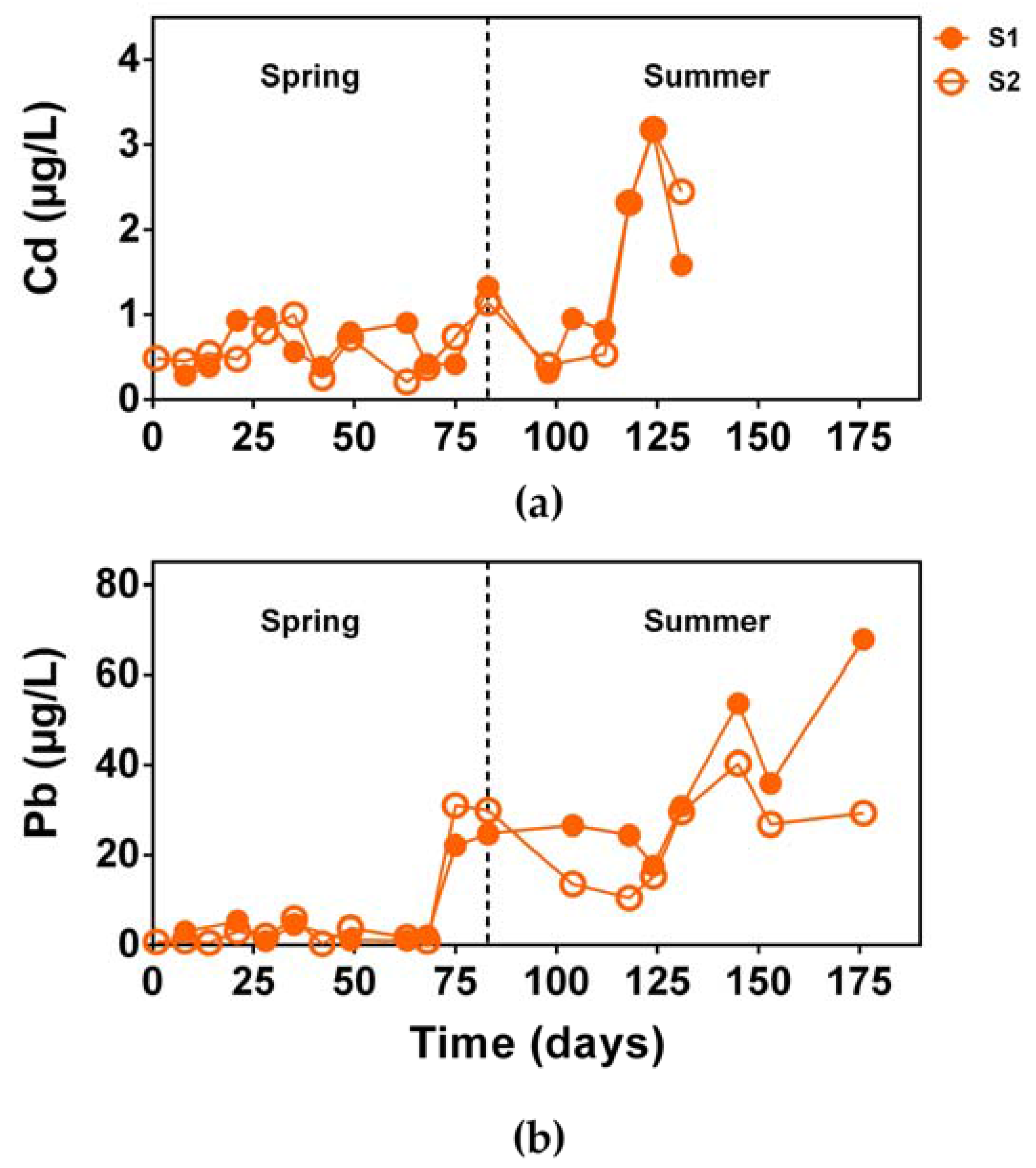
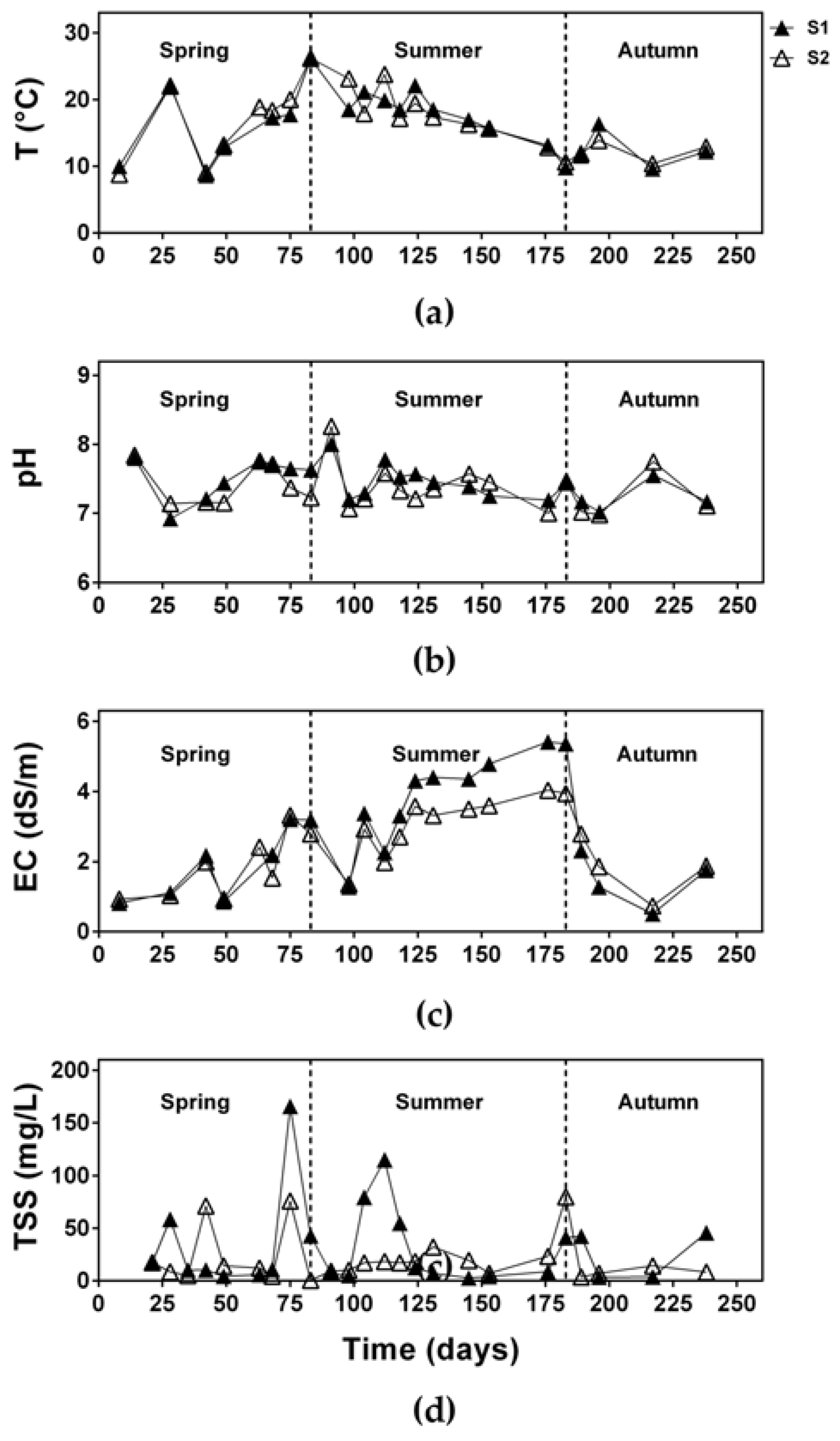
3.2. Surface Water Quality
3.2.1. Water Quality Indicators
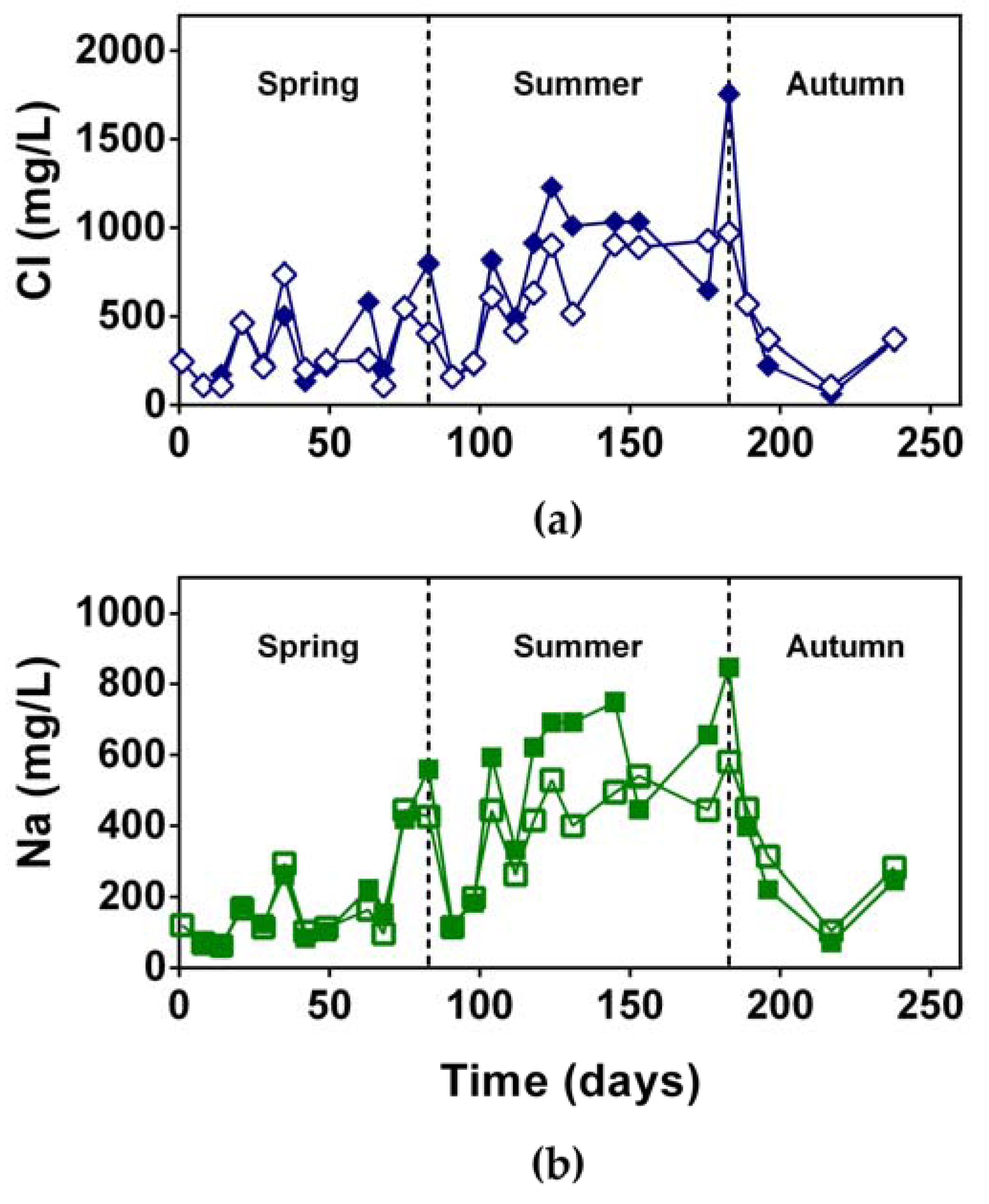
3.2.2. NaCl Concentration and Removal Efficiency
3.2.3. Trace Metal Concentration and Removal Efficiency
4. Conclusions
Acknowledgments
Author Contributions
Conflicts of Interest
References
- Zhang, W.; Zhang, S.; Wan, C.; Yue, D.; Ye, Y.; Wang, X. Source diagnostics of polycyclic aromatic hydrocarbons in urban road runoff, dust, rain and canopy throughfall. Environ. Pollut. 2008, 153, 594–601. [Google Scholar] [CrossRef] [PubMed]
- Kayhanian, M.; Singh, A.; Suverkropp, C.; Borroum, S. Impact of annual average daily traffic on highway runoff pollutant concentrations. J. Environ. Eng. 2003, 129, 975–990. [Google Scholar] [CrossRef]
- Environment Canada. Five-Year Review of Progress: Code of Practice for the Environmental Management of Road Salts. March 31; Environment Canada: Gatineau, QC, Canada, 2012. [Google Scholar]
- Gouvernement du Québec. Stratégie Québécoise Pour une Gestion Environnementale des sels de Voirie. Bilan Québécois Annuel 2012–2013; Gouvernement du Québec: Quebec City, QC, Canada, 2014. [Google Scholar]
- Meriano, M.; Eyles, N.; Howard, K.W.F. Hydrogeological impacts of road salt from Canada’s busiest highway on a Lake Ontario watershed (Frenchman’s Bay) and lagoon, City of Pickering. J. Contam. Hydrol. 2009, 107, 66–81. [Google Scholar] [CrossRef] [PubMed]
- Cañedo-Argüelles, M.; Kefford, B.J.; Piscart, C.; Prat, N.; Schäfer, R.B.; Schulz, C.-J.J. Salinisation of rivers: An urgent ecological issue. Environ. Pollut. 2013, 173, 157–167. [Google Scholar] [CrossRef] [PubMed]
- Novotny, E.V.; Stefan, H.G. Road Salt Impact on Lake Stratification and Water Quality. J. Hydraul. Eng. 2012, 346, 1069–1080. [Google Scholar] [CrossRef]
- Daley, M.L.; Potter, J.D.; McDowell, W.H. Salinization of urbanizing New Hampshire streams and groundwater: Effects of road salt and hydrologic variability. J. N. Am. Benthol. Soc. 2009, 28, 929–940. [Google Scholar] [CrossRef]
- Morteau, B.; Triffault-Bouchet, G.; Galvez, R.; Martel, L.; Leroueil, S.; Galvez, R.; Dyer, M.; Dean, S.W. Treatment of Salted Road Runoffs Using Typha latifolia, Spergularia canadensis, and Atriplex patula: A Comparison of their Salt Removal Potential. J. ASTM Int. 2009, 6. [Google Scholar] [CrossRef]
- Galvez-Cloutier, R.; Saminathan, S.K.M.; Boillot, C.; Triffaut-Bouchet, G.; Bourget, A.; Soumis-Dugas, G. An Evaluation of Several In-Lake Restoration Techniques to Improve the Water Quality Problem (Eutrophication) of Saint-Augustin Lake, Quebec, Canada. Environ. Manag. 2012, 49, 1037–1053. [Google Scholar] [CrossRef] [PubMed]
- Bäckström, M.; Karlsson, S.; Bäckman, L.; Folkeson, L.; Lind, B. Mobilisation of heavy metals by deicing salts in a roadside environment. Water Res. 2004, 38, 720–732. [Google Scholar] [CrossRef] [PubMed]
- Kelting, D.L.; Laxson, C.L. Review of Effects and Costs of Road De-Icing with Recommendations for Winter Road Management in the Adirondack Park; Paul Smith’s College: Saranac Lake, NY, USA, 2010. [Google Scholar]
- Mayer, T.; Snodgrass, W.J.; Morin, D. Spatial characterization of the occurrence of road salts and their environmental concentrations as chlorides in Canadian surface waters and benthic sediments. Water Qual. Res. J. Can. 1999, 34, 545–574. [Google Scholar]
- Environment Canada and Health Canada. Canadian Environmental Protection Act, 1999. Priority Substances List Assessment Report. Road Salts; Environment Canada and Health Canada: Ottawa, ON, Canada, 2001. [Google Scholar]
- Marsalek, J. Road salts in urban stormwater: An emerging issue in stormwater management in cold climates. Water Sci. Technol. 2003, 48, 61–70. [Google Scholar] [PubMed]
- Boillot, C.; Triffault-Bouchet, G.; Soumis-Dugas, G.; Martel, L.; Galvez, R. Évaluation de la Compatibilité Ecologique d’une Technique de Restauration Pour lacs Eutrophes vis-à-vis du lac Saint-Augustin et de la Baie Missisquoi. Ministère du Développement Durable, de l’Environnement et des Parcs du Québec et Université Laval; Laval University: Quebec City, QC, Canada, 2010. [Google Scholar]
- Pienitz, R.; Roberge, K.; Vincent, W.F. Three hundred years of human-induced change in an urban lake: Paleolimnological analysis of Lac Saint-Augustin, Québec City, Canada. Can. J. Bot. 2006, 84, 303–320. [Google Scholar] [CrossRef]
- Bergeron, M.; Corbeil, C.; Arsenault, S. Diagnose Ecologique du lac Saint-Augustin. Document Préparé pour la Municipalité de Saint-Augustin-de-Desmaures par EXXEP Environnement, Québec, 70 Pages et 6 Annexes; EXXEP Environnement: Quebec City, QC, Canada, 2002. [Google Scholar]
- Galvez-Cloutier, R.; Brin, M.-E.; Dominguez, G.; Leroueil, S.; Arsenault, S. Quality evaluation of eutrophic sediments at St Augustin Lake, Quebec, Canada. ASTM Int. 2003, 1442, 35–52. [Google Scholar]
- Galvez-Cloutier, R.; Leroueil, S.; Pérez-Arzola, J.C. Le lac Saint-Augustin, sa Problématique d’eutrophisation et le lien avec les produits d’entretien de l’autoroute Félix-Leclerc. Rapport technique final 03605’3_06 présenté au ministère des Transports du Québec. Volet II : Évaluation de la qualité des eau; Laval University: Quebec City, QC, Canada, 2006. [Google Scholar]
- Roberge, K.; Pienitz, R.; Arsenault, S. Eutrophisation rapide du lac Saint-Augustin, Québec: Étude paléolimnologique pour une reconstitution de la qualité de l’eau. Nat. Can. 2002, 126, 68–82. [Google Scholar]
- Gouvernment of Canada. Historical Data. Available online: http://climate.weather.gc.ca/historical_data/search_historic_data_e.html (accessed on 16 March 2013).
- Consortium Dessau-Soprin. Étude D’opportunité de L’autoroute Félix-Leclerc sur le Territoire de la Ville de Québec; Dessau-Soprin: Quebec City, QC, Canada, 2004. [Google Scholar]
- Galvez, R.; Leroueil, S.; Triffault-Bouchet, G.; Martel, L.; Morteau, B. Natural geo-filter bed and halophyte wetland: An eco-engineering system to mitigate saline highway runoff impacts. In IASTED Technology Conferences; Alhajj, S.S., Leung, V.C.M., Petela, R., Saif, M., Thring, R., Eds.; ACTA Press: Banff, AB, Canada, 2010. [Google Scholar]
- Messaoud, H. Aspects Hydrogéologiques et Suivi de la Qualité des Eaux Souterraines du Bassin Versant du lac Saint-Augustin: Impacts des sels de Déglaçage. Master’s Thesis, Laval University, Quebec City, QC, Canada, 2015. [Google Scholar]
- American Public Health Association (APHA). Standard Methods for the Examination of Water and Wastewater, 20th ed.; American Public Health Association: Washington, DC, USA, 1998. [Google Scholar]
- Talbot Poulin, M.C.; Comeau, G.; Tremblay, Y.; Therrien, R.; Nadeau, M.M.; Lemieux, J.M.; Molson, J.; Fortier, R.; Therrien, P.; Lamarche, L.; et al. Projet D’acquisition de Connaissances sur les Eaux Souterraines du Territoire de la Communauté Métropolitaine de Québec, Rapport Final; Laval University: Quebec City, QC, Canada, 2013. [Google Scholar]
- McConnell, H.H.; Lewis, J. Add Salt to Taste. Environ. Sci. Policy Sustain. Dev. 1972, 14, 38–44. [Google Scholar] [CrossRef]
- Government of Canada. Guidelines for Canadian Drinking Water Quality: Guideline Technical Document—Chloride; Health Canada: Ottawa, ON, Canada, 1987.
- Government of Canada. Guidelines for Canadian Drinking Water Quality: Guideline Technical Document—Sodium; Health Canada: Ottawa, ON, Canada, 1992.
- Health Canada. Guidelines for Canadian Drinking Water Quality—Summary Table. Water and Air Quality Bureau, Healthy Enviroments and Consumer Safety Branch; Health Canada: Ottawa, ON, Canada, 2014. [Google Scholar]
- Tchobanoglous, G.; Burton, F.L.; Stensel, H.D.; Eddy, M.; Metcalf & Eddy, Inc. Wastewater Engineering. Treatment and Reuse, 4th ed.; McGraw-Hil: New York, NY, USA, 2003. [Google Scholar]
- Helmreich, B.; Hilliges, R.; Schriewer, A.; Horn, H. Runoff pollutants of a highly trafficked urban road—Correlation analysis and seasonal influences. Chemosphere 2010, 80, 991–997. [Google Scholar] [CrossRef] [PubMed]
- Kuoppamäki, K.; Setälä, H.; Rantalainen, A.-L.; Kotze, D.J. Urban snow indicates pollution originating from road traffic. Environ. Pollut. 2014, 195, 56–63. [Google Scholar] [CrossRef] [PubMed]
- Hallberg, M.; Renman, G.; Lundbom, T. Seasonal variations of ten metals in highway runoff and their partition between dissolved and particulate matter. Water Air Soil Pollut. 2007, 181, 183–191. [Google Scholar] [CrossRef]
- Kayhanian, M.; Suverkropp, C.; Ruby, A.; Tsay, K. Characterization and prediction of highway runoff constituent event mean concentration. J. Environ. Manag. 2007, 85, 279–295. [Google Scholar] [CrossRef] [PubMed]
- Aryal, R.K.; Furumai, H.; Nakajima, F.; Boller, M. Dynamic behavior of fractional suspended solids and particle-bound polycyclic aromatic hydrocarbons in highway runoff. Water Res. 2005, 39, 5126–5134. [Google Scholar] [CrossRef] [PubMed]
- Lee, J.H.; Bang, K.W. Characterization of urban stormwater runoff. Water Res. 2000, 34, 1773–1780. [Google Scholar] [CrossRef]
- Ministère Développement Durable Environnement Faunes des Parcs (MDDEFP). Critères de Qualité de l’eau de Surface 2013, 3e Edition, Québec, Direction du Suivi de l’état de L’environnement; Gouvernement du Québec: Quebec City, QC, Canada, 2013. [Google Scholar]
- United States Environmental Protection Agency (USEPA). National Recommended Water Quality Criteria—Aquatic Life Criteria Table; US Environmental Protection Agency: Washington, DC, USA, 2016. [Google Scholar]
- Li, F.; Zhang, Y.; Fan, Z.; Oh, K. Accumulation of De-icing Salts and Its Short-Term Effect on Metal Mobility in Urban Roadside Soils. Bull. Environ. Contam. Toxicol. 2015, 94, 525–531. [Google Scholar] [CrossRef] [PubMed]
- Rhodes, A.L.; Newton, R.M.; Pufall, A. Influences of land use on water quality of a diverse New England watershed. Environ. Sci. Technol. 2001, 35, 3640–3645. [Google Scholar] [CrossRef] [PubMed]
- Cooper, C.A.; Mayer, P.M.; Faulkner, B.R. Effects of road salts on groundwater and surface water dynamics of sodium and chloride in an urban restored stream. Biogeochemistry 2014, 121, 149–166. [Google Scholar] [CrossRef]
- Harada, J.; Inoue, T.; Kato, K.; Uraie, N.; Sakuragi, H. Performance evaluation of hybrid treatment wetland for six years of operation in cold climate. Environ. Sci. Pollut. Res. 2015, 22, 12861–12869. [Google Scholar] [CrossRef] [PubMed]
- Bäckström, M.; Nilsson, U.; Håkansson, K.; Allard, B.; Karlsson, S. Speciation of heavy metals in road runoff and roadside total deposition. Water Air Soil Pollut. 2003, 147, 343–366. [Google Scholar] [CrossRef]
- Valtanen, M.; Sillanpää, N.; Setälä, H. The effects of urbanization on runoff pollutant concentrations, loadings and their seasonal patterns under cold climate. Water Air Soil Pollut. 2014, 225. [Google Scholar] [CrossRef]
- Farrell, A.C.; Scheckenberger, R.B. An assessment of long-term monitoring data for constructed wetlands for urban highway runoff control. Water Qual. Res. J. Can. 2003, 38, 283–315. [Google Scholar]
- Wong, T.; Breen, P.; Lloyd, S. Water Sensitive Road Design—Design Options for Improving Stormwater Quality of Road Runoff. Techical Report 00/1. Cooperative Research Centre for Catchment Hydrology; Cooperative Research Centre for Catchment Hydrology: Victoria, Australia, 2000. [Google Scholar]
- Glenn, D.W.; Sansalone, J.J. Accretion and Partitioning of Heavy Metals Associated with Snow Exposed to Urban Traffic and Winter Storm Maintenance Activities II. J. Environ. Eng. 2002, 128, 167–185. [Google Scholar] [CrossRef]
- Westerlund, C.; Viklander, M.; Bäckström, M. Seasonal variations in road runoff quality in Lulea, Sweden. Water Sci. Technol. 2003, 48, 93–101. [Google Scholar]


| Well | Parameters | T | pH | EC | WL | Cl− | Na+ | Ca2+ | Mg2+ | K+ | HCO3− | SO42− |
|---|---|---|---|---|---|---|---|---|---|---|---|---|
| G1 | T | 1 | 0.674 ** | 0.788 *** | 0.611 * | −0.458 | −0.252 | 0.696 ** | 0.506 | 0.588 * | 0.813 *** | 0.472 |
| pH | 1 | 0.549 * | 0.234 | −0.395 | −0.192 | 0.553 * | 0.458 | 0.251 | 0.368 | 0.416 | ||
| EC | 1 | 0.368 | −0.514 * | −0.224 | 0.968 *** | 0.366 | 0.708 ** | 0.879 *** | 0.660 ** | |||
| WL | 1 | 0.075 | 0.057 | 0.176 | 0.680 ** | 0.568 * | 0.535 * | 0.067 | ||||
| Cl− | 1 | 0.547 * | −0.544 * | −0.398 | −0.252 | −0.437 | −0.438 | |||||
| Na+ | 1 | −0.321 | −0.344 | 0.056 | −0.336 | 0.092 | ||||||
| G2 | T | 1 | 0.309 | −0.220 | 0.167 | 0.021 | −0.367 | −0.105 | −0.247 | −0.260 | −0.122 | 0.330 |
| pH | 1 | −0.593 * | 0.474 | 0.413 | −0.146 | −0.503 | −0.672 ** | −0.207 | −0.593 * | −0.145 | ||
| EC | 1 | −0.109 | 0.232 | 0.335 | 0.532 * | 0.520 * | 0.356 | 0.930 *** | −0.157 | |||
| WL | 1 | 0.506 | −0.162 | −0.201 | −0.168 | 0.350 | −0.137 | −0.009 | ||||
| Cl− | 1 | 0.307 | −0.269 | −0.150 | 0.258 | 0.063 | −0.085 | |||||
| Na+ | 1 | −0.048 | 0.230 | 0.311 | 0.014 | 0.024 | ||||||
| G3 | T | 1 | −0.270 | 0.472 | 0.554 * | 0.563 * | 0.148 | 0.392 | 0.400 | −0.440 | −0.198 | 0.283 |
| pH | 1 | −0.876 *** | −0.727 ** | −0.903 *** | −0.442 | −0.871 *** | −0.725 ** | 0.100 | 0.350 | −0.905 *** | ||
| EC | 1 | 0.808 *** | 0.951 *** | 0.405 | 0.968 *** | 0.889 *** | −0.201 | −0.076 | 0.916 *** | |||
| WL | 1 | 0.822 *** | 0.337 | 0.769 ** | 0.668 ** | −0.087 | −0.226 | 0.778 ** | ||||
| Cl− | 1 | 0.508 | 0.889 *** | 0.754 ** | −0.288 | −0.293 | 0.872 *** | |||||
| Na+ | 1 | 0.304 | 0.143 | −0.089 | −0.518 * | 0.466 | ||||||
| G4 | T | 1 | −0.259 | −0.349 | 0.334 | −0.323 | −0.133 | −0.499 | −0.185 | 0.378 | −0.328 | 0.412 |
| pH | 1 | 0.615 * | 0.618 * | 0.605 * | 0.542 * | 0.399 | 0.283 | −0.238 | 0.258 | −0.446 | ||
| EC | 1 | 0.280 | 0.787 *** | 0.881 *** | 0.495 | 0.447 | −0.219 | 0.591 * | −0.510 | |||
| WL | 1 | 0.251 | 0.387 | 0.035 | 0.366 | 0.046 | 0.035 | −0.438 | ||||
| Cl− | 1 | 0.551 * | 0.367 | 0.458 | −0.466 | 0.120 | −0.342 | |||||
| Na+ | 1 | 0.295 | 0.534 * | −0.109 | 0.469 | −0.530 * | ||||||
| G5 | T | 1 | 0.059 | 0.287 | 0.454 | 0.287 | 0.156 | 0.302 | 0.255 | 0.138 | 0.233 | 0.238 |
| pH | 1 | −0.661 ** | −0.600 * | −0.694 ** | −0.510 | −0.660 ** | −0.681 ** | 0.059 | −0.528 * | −0.689 ** | ||
| EC | 1 | 0.946 *** | 0.973 *** | 0.818 *** | 0.989 *** | 0.950 *** | 0.295 | 0.937 *** | 0.978 *** | |||
| WL | 1 | 0.941 *** | 0.704 ** | 0.930 *** | 0.905 *** | 0.145 | 0.897 *** | 0.886 *** | ||||
| Cl− | 1 | 0.751 ** | 0.944 *** | 0.952 *** | 0.276 | 0.888 *** | 0.952 *** | |||||
| Na+ | 1 | 0.788 *** | 0.777 ** | 0.318 | 0.700 ** | 0.833 *** |
| Parameters | Influent (S1) | Effluent (S2) | |||||||
|---|---|---|---|---|---|---|---|---|---|
| Units | Min | Max | Mean | SEM | Min | Max | Mean | SEM | |
| T | °C | 9.1 | 17.5 | 14.1 | 1.8 | 8.9 | 19.2 | 16.3 | 2.5 |
| pH | - | 7.4 | 8.2 | 7.8 | 0.1 | 7.1 | 8.2 | 7.7 | 0.2 |
| EC | dS/m | 0.7 | 2.8 | 1.9 | 0.4 | 0.6 | 2.2 | 1.1 | 0.3 |
| TSS | µg/L | 2.2 | 386.8 | 194.5 | 192.3 | 12.4 | 35.8 | 24.1 | 11.7 |
| Sampling Points | Parameters | T | pH | EC | TSS | Cl | Na | Cd | Pb |
|---|---|---|---|---|---|---|---|---|---|
| S1 vs. S1 | T | 1 | 0.224 | 0.169 | 0.292 | 0.221 | 0.308 | 0.481 | −0.069 |
| pH | 1 | −0.230 | 0.149 | 0.002 | −0.063 | 0.059 | −0.293 | ||
| EC | 1 | 0.153 | 0.787 *** | 0.880 *** | 0.606 ** | 0.857 *** | |||
| TSS | 1 | 0.092 | 0.155 | −0.120 | −0.045 | ||||
| Cl | 1 | 0.922 *** | 0.852 *** | 0.611 * | |||||
| Na | 1 | 0.766 *** | 0.810 *** | ||||||
| Cd | 1 | 0.481 | |||||||
| Pb | 1 | ||||||||
| S2 vs. S2 | T | 1 | 0.094 | 0.073 | −0.321 | −0.014 | 0.122 | 0.117 | 0.292 |
| pH | 1 | −0.033 | −0.025 | −0.303 | −0.352 | −0.282 | −0.190 | ||
| EC | 1 | 0.358 | 0.913 *** | 0.914 *** | 0.670 * | 0.810 *** | |||
| TSS | 1 | 0.226 | 0.227 | −0.066 | 0.140 | ||||
| Cl | 1 | 0.908 *** | 0.757 ** | 0.701 ** | |||||
| Na | 1 | 0.775 *** | 0.843 *** | ||||||
| Cd | 1 | 0.514 | |||||||
| Pb | 1 | ||||||||
| S1 vs. S2 | T | 0.925 *** | −0.034 | 0.177 | −0.383 | 0.119 | 0.264 | 0.426 | 0.313 |
| pH | 0.335 | 0.815 ** | 0.108 | 0.046 | −0.223 | −0.201 | 0.005 | −0.083 | |
| EC | 0.026 | −0.349 | 0.898 *** | 0.384 | 0.770 *** | 0.843 *** | 0.726 ** | 0.807 *** | |
| TSS | 0.372 | −0.077 | 0.118 | 0.376 | 0.059 | 0.233 | −0.081 | 0.189 | |
| Cl | 0.109 | −0.110 | 0.852 *** | 0.329 | 0.850 *** | 0.871 *** | 0.869 *** | 0.718 ** | |
| Na | 0.157 | −0.231 | 0.902 *** | 0.277 | 0.859 *** | 0.918 *** | 0.862 *** | 0.824 *** | |
| Cd | 0.201 | −0.229 | 0.607 * | −0.188 | 0.698 ** | 0.679 ** | 0.914 *** | 0.356 | |
| Pb | −0.132 | −0.269 | 0.820 *** | 0.222 | 0.755 ** | 0.763 ** | 0.699 * | 0.846 *** |
© 2016 by the authors; licensee MDPI, Basel, Switzerland. This article is an open access article distributed under the terms and conditions of the Creative Commons Attribution (CC-BY) license (http://creativecommons.org/licenses/by/4.0/).
Share and Cite
Guesdon, G.; De Santiago-Martín, A.; Raymond, S.; Messaoud, H.; Michaux, A.; Roy, S.; Galvez, R. Impacts of Salinity on Saint-Augustin Lake, Canada: Remediation Measures at Watershed Scale. Water 2016, 8, 285. https://doi.org/10.3390/w8070285
Guesdon G, De Santiago-Martín A, Raymond S, Messaoud H, Michaux A, Roy S, Galvez R. Impacts of Salinity on Saint-Augustin Lake, Canada: Remediation Measures at Watershed Scale. Water. 2016; 8(7):285. https://doi.org/10.3390/w8070285
Chicago/Turabian StyleGuesdon, Gaëlle, Ana De Santiago-Martín, Sébastien Raymond, Hamdi Messaoud, Arthur Michaux, Samuel Roy, and Rosa Galvez. 2016. "Impacts of Salinity on Saint-Augustin Lake, Canada: Remediation Measures at Watershed Scale" Water 8, no. 7: 285. https://doi.org/10.3390/w8070285
APA StyleGuesdon, G., De Santiago-Martín, A., Raymond, S., Messaoud, H., Michaux, A., Roy, S., & Galvez, R. (2016). Impacts of Salinity on Saint-Augustin Lake, Canada: Remediation Measures at Watershed Scale. Water, 8(7), 285. https://doi.org/10.3390/w8070285