
An Assessment of the Effectiveness of Tree-Based Models for Multi-Variate Flood Damage Assessment in Australia


Abstract
:
1. Introduction
2. Study Area and Data
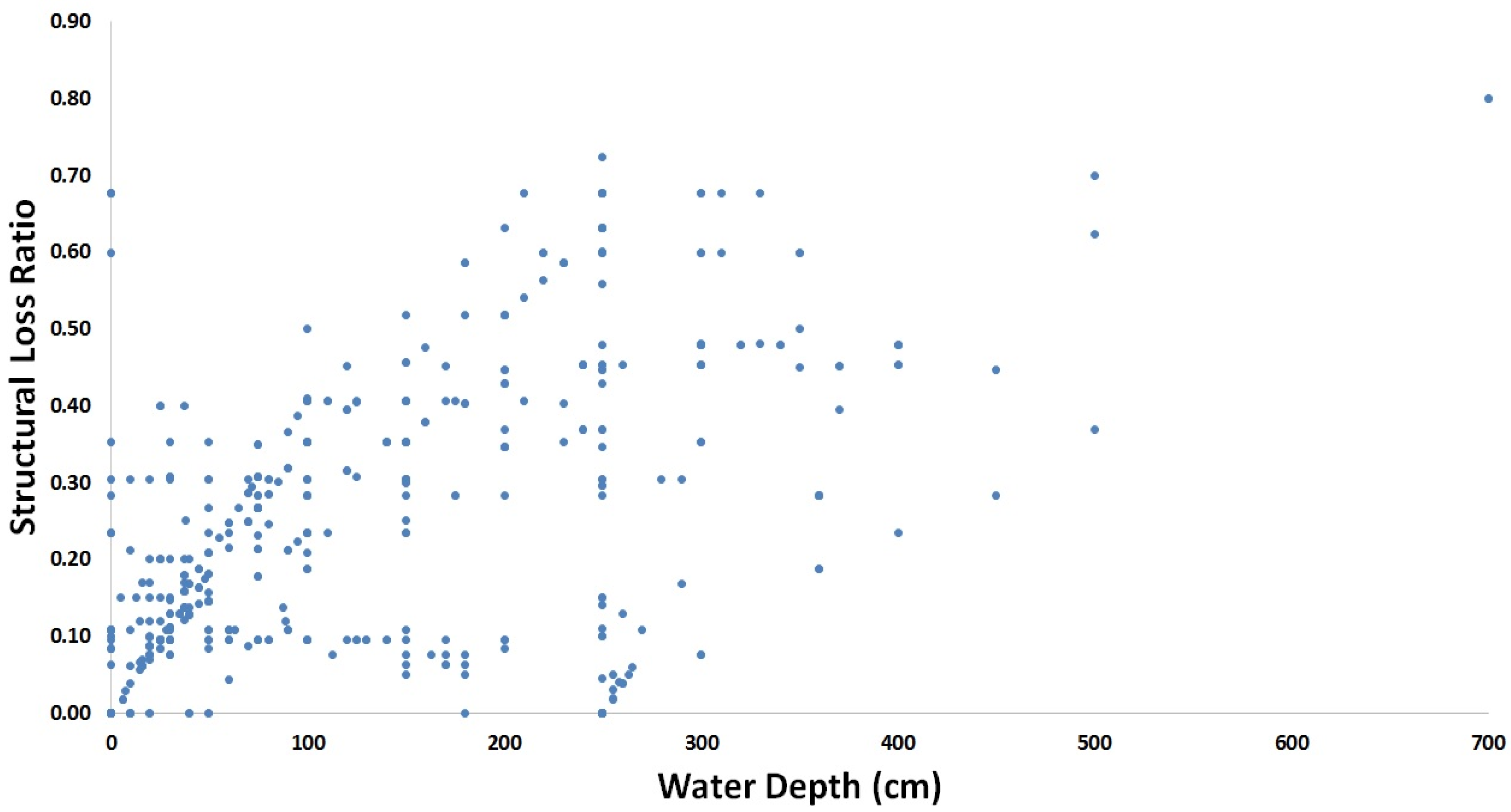
- Water depth and water contamination: this information was collected in two post-disaster surveys. The value of water depth fluctuated between 0 cm and 700 cm above ground. However, for 96% of buildings, this attribute was equal to or less than 350 cm. Also, the existence of sewage, biological, or chemical contamination has been checked and reported by visual inspection and smell. Accordingly, water contamination was ranked based on the reported material and the existing chemical hazards, from 0 (no contamination) to 2 (chemical contamination), with 1 representing only sewage contamination.
- Flow velocity: flow velocity was assessed according to the comments of inspectors about the amount of water penetration inside of buildings, the volume of deposited materials, and the type of sediment next to the house (mud, sand, gravel or stone). Afterwards, this information was transformed and ranked as calm (1: no deposit or only mud sediment), medium (2: sand sediment or a considerable amount of water penetration), or high (3: gravel or stone sediment or high volume of deposits) flow velocity.
- Emergency measures: the dataset provides information about whether or not people undertook any action against water infiltration, e.g., pumping water out or cut-off of electricity supply. Subsequently, these actions were ranked from 0 (no measure was undertaken) to 3 (many measures were undertaken), with 1 representing that only water was pumped out, and 2 representing that only electricity supply was cut off. The “cut-off of electricity supply” measure had a greater weight due to the high value of electrical equipment [2].
- Precaution measures: the indicators of precaution measures were defined and ranked based on the construction type (3: high-set open under, 2: low-set with suspended floor, or 1: high-set enclosed under or slab on ground); protection of utilities and power system against water impacts (1: no protection, 2: protected); availability of solar-panel power provider (1: not available, 2: available); and the number of building storeys (1: one-storey buildings, 2: two-storey buildings). Eventually, precaution measure indicators were calculated and weighted by multiplying the above ranks.
- Flood experience: the areas of study have experienced a variety of flood events in recent years [2,52]. Therefore, this parameter has been assessed and averaged according to the length of residency. Overall, about 11% of households moved into the areas one year or less before the events, weighted 1. About 31% of families settled there in the last five years, weighted as 2. Residents with more than five years length of residency were weighted 3.
- Building quality: this item is a function of age (i.e., constructed pre- or post-1981) and material (e.g., timber, brick, concrete, or metal) of buildings. Age of buildings was weighted 1 if the structure was constructed pre-1981 and 2 if it was constructed post-1981. Also, the resistance of different materials against impacts of water is judged and ranked: 1 for timber, 2 for brick, and 3 for concrete or metal, according to the Australian building guidelines for flood prone areas [53]. Finally, this candidate predictor is defined by multiplying the weight of age by the weight of the material.
- The value and floor space of building: for every building, the value was calculated by multiplying the total area reported by the inspectors by the average replacement value per square metre extracted from the national exposure information system of Australia [51]. In this study, besides considering the area of the buildings, the contribution of the residents’ density with the extent of losses has been taken into account. Accordingly, floor space of the building was calculated per person, by dividing the total area by the number of residents.
- Socioeconomic status: this category includes information about ownership status and monthly income (i.e., low: $1–$599, middle: $600–$1,999, or high: greater than $2,000). Also, it represents buildings whose residents need special attention (i.e., aged less than five or more than 65; needing assistance with a core activity; or do not speak English well) or low education residents (i.e., the highest educational attainment of all building residents is year 11 or below).
3. Statistical Methods
3.1. Regression Trees
3.2. Bagging Decision Trees
3.3. Comparing the Performance of the Tree-Based Models with FLFArs
4. Results and Discussion
4.1. Importance and Interaction of the Damage Influencing Parameters
4.1.1. Regression Trees
4.1.2. Bagging Decision Trees
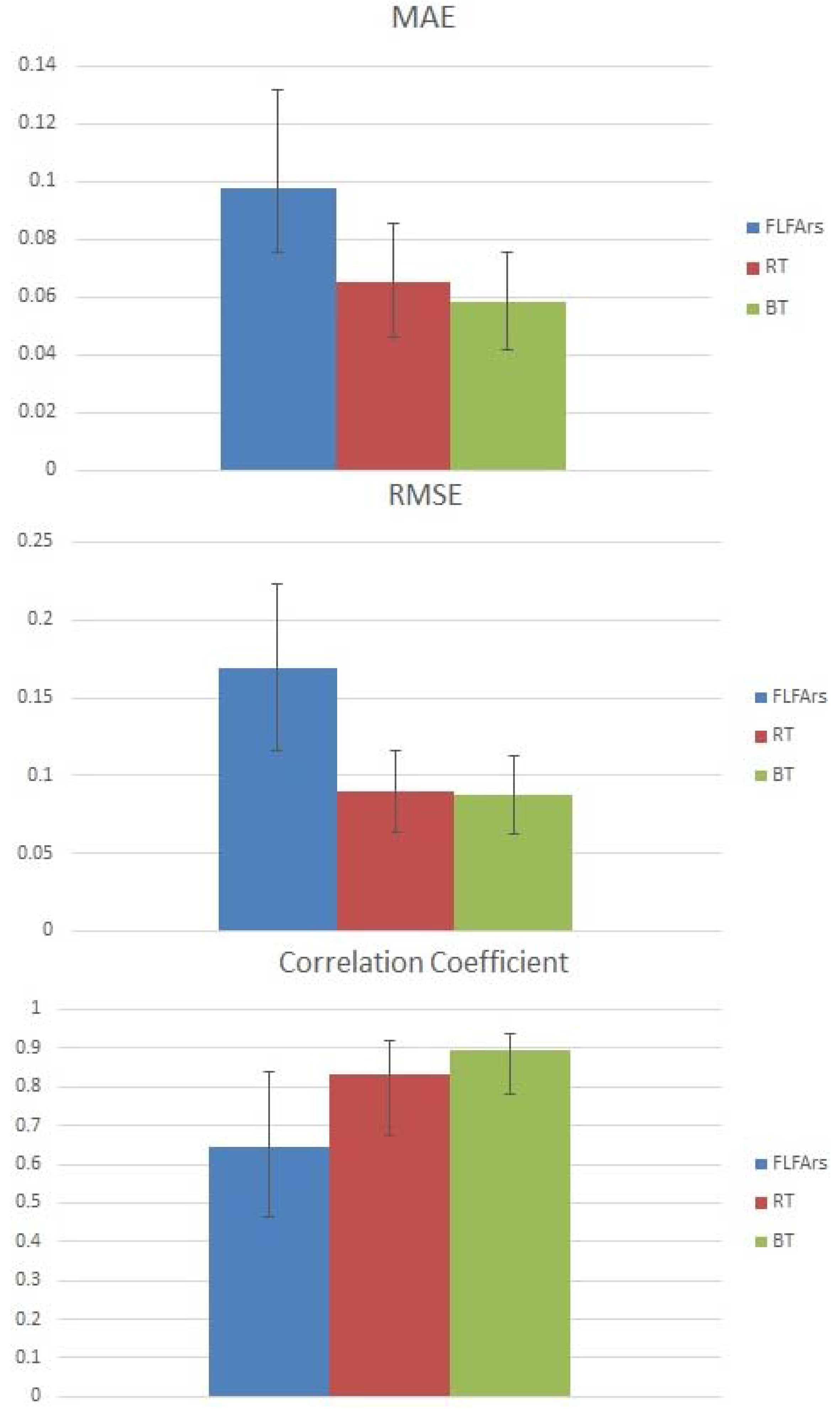
4.1.3. Performance of the Applied Damage Models
5. Conclusions
Acknowledgments
Author Contributions
Conflicts of Interest
References
- Elmer, F.; Hoymann, J.; Düthmann, D.; Vorogushyn, S.; Kreibich, H. Drivers of flood risk change in residential areas. Nat. Hazards Earth Syst. Sci. 2012, 12, 1641–1657. [Google Scholar] [CrossRef]
- Hasanzadeh Nafari, R.; Ngo, T.; Lehman, W. Calibration and validation of FLFArs—A new flood loss function for Australian residential structures. Nat. Hazards Earth Syst. Sci. 2016, 16, 15–27. [Google Scholar] [CrossRef]
- Kundzewicz, Z.W.; Ulbrich, U.; Brücher, T.; Graczyk, D.; Krüger, A.; Leckebusch, G.C.; Menzel, L.; Pińskwar, I.; Radziejewski, M.; Szwed, M. Summer floods in Central Europe—Climate change track? Nat. Hazards 2005, 36, 165–189. [Google Scholar] [CrossRef]
- Box, P.; Thomalla, F.; van den Honert, R. Flood risk in Australia: Whose responsibility is it, anyway? Water 2013, 5, 1580–1597. [Google Scholar] [CrossRef]
- Economic Costs of Natural Disasters in Australia. Available online: https://bitre.gov.au/publications/2001/files/report_103.pdf (accessed on 4 July 2016).
- Hasanzadeh Nafari, R.; Ngo, T.; Lehman, W. Development and evaluation of FLFAcs—A new Flood Loss Function for Australian commercial structures. Int. J. Dis. Risk Reduct. 2016, 17, 13–23. [Google Scholar] [CrossRef]
- Kreibich, H.; Seifert, I.; Merz, B.; Thieken, A.H. Development of FLEMOcs—A new model for the estimation of flood losses in the commercial sector. Hydrol. Sci. J. 2010, 55, 1302–1314. [Google Scholar] [CrossRef]
- Schröter, K.; Kreibich, H.; Vogel, K.; Riggelsen, C.; Scherbaum, F.; Merz, B. How useful are complex flood damage models? Water Resour. Res. 2014, 50, 3378–3395. [Google Scholar] [CrossRef]
- Van Ootegem, L.; Verhofstadt, E.; van Herck, K.; Creten, T. Multivariate pluvial flood damage models. Environ. Impact Assess. Rev. 2015, 54, 91–100. [Google Scholar] [CrossRef]
- Emanuelsson, M.A.E.; Mcintyre, N.; Hunt, C.F.; Mawle, R.; Kitson, J.; Voulvoulis, N. Flood risk assessment for infrastructure networks. J. Flood Risk Manag. 2014, 7, 31–41. [Google Scholar] [CrossRef]
- Merz, B.; Kreibich, H.; Schwarze, R.; Thieken, A. Review article “assessment of economic flood damage”. Nat. Hazards Earth Syst. Sci. 2010, 10, 1697–1724. [Google Scholar] [CrossRef]
- Chen, A.S.; Hammond, M.J.; Djordjević, S.; Butler, D.; Khan, D.M.; Veerbeek, W. From hazard to impact: Flood damage assessment tools for mega cities. Nat. Hazards 2016, 82, 857–890. [Google Scholar] [CrossRef]
- Olsen, A.S.; Zhou, Q.; Linde, J.J.; Arnbjerg-Nielsen, K. Comparing methods of calculating expected annual damage in urban pluvial flood risk assessments. Water 2015, 7, 255–270. [Google Scholar] [CrossRef]
- Bubeck, P.; Aerts, J.C.J.H.; de Moel, H.; Kreibich, H. Preface: Flood-risk analysis and integrated management. Nat. Hazards Earth Syst. Sci. 2016, 16, 1005–1010. [Google Scholar] [CrossRef]
- Merz, B.; Kreibich, H.; Lall, U. Multi-variate flood damage assessment: A tree-based data-mining approach. Nat. Hazards Earth Syst. Sci. 2013, 13, 53–64. [Google Scholar] [CrossRef]
- Morita, M. Flood risk impact factor for comparatively evaluating the main causes that contribute to flood risk in urban drainage areas. Water 2014, 6, 253–270. [Google Scholar] [CrossRef]
- De Moel, H.; Jongman, B.; Kreibich, H.; Merz, B.; Penning-Rowsell, E.; Ward, P.J. Flood risk assessments at different spatial scales. Mitig. Adapt. Strateg. Glob. Chang. 2015, 20, 865–890. [Google Scholar] [CrossRef]
- Handmer, J.; Abrahams, J.; Betts, R.; Dawson, M. Towards a consistent approach to disaster loss assessment across Australia. Aust. J. Emerg. Manag. 2005, 20, 10–18. [Google Scholar]
- Gall, M.; Borden, K.A.; Cutter, S.L. When do losses count? Six fallacies of natural hazards loss data. Bull. Am. Meteorol. Soc. 2009, 90, 799–809. [Google Scholar] [CrossRef]
- Gerl, T.; Bochow, M.; Kreibich, H. Flood Damage Modeling on the Basis of Urban Structure Mapping Using High-Resolution Remote Sensing Data. Water 2014, 6, 2367–2393. [Google Scholar] [CrossRef]
- Wind, H.G.; Nierop, T.M.; de Blois, C.J.; de Kok, J.L. Analys is of flood damages from the 1993 and 1995 Meuse floods. Water Resour. Res. 1999, 35, 3459–3465. [Google Scholar] [CrossRef]
- Jonkman, S.; Dawson, R. Issues and Challenges in Flood Risk Management—Editorial for the Special Issue on Flood Risk Management. Water 2012, 4, 785–792. [Google Scholar] [CrossRef]
- Meyer, V.; Becker, N.; Markantonis, V.; Schwarze, R.; van den Bergh, J.C.J.M.; Bouwer, L.M.; Bubeck, P.; Ciavola, P.; Genovese, E.; Green, C.; et al. Review article: Assessing the costs of natural hazards-state of the art and knowledge gaps. Nat. Hazards Earth Syst. Sci. 2013, 13, 1351–1373. [Google Scholar] [CrossRef]
- Thieken, A.H.; Müller, M.; Kreibich, H.; Merz, B. Flood damage and influencing factors: New insights from the August 2002 flood in Germany. Water Resour. Res. 2005, 41, 1–16. [Google Scholar] [CrossRef]
- André, C.; Monfort, D.; Bouzit, M.; Vinchon, C. Contribution of insurance data to cost assessment of coastal flood damage to residential buildings: Insights gained from Johanna (2008) and Xynthia (2010) storm events. Nat. Hazards Earth Syst. Sci. 2013, 13, 2003–2012. [Google Scholar] [CrossRef]
- Chinh, D.; Gain, A.; Dung, N.; Haase, D.; Kreibich, H. Multi-Variate Analyses of Flood Loss in Can Tho City, Mekong Delta. Water 2015, 8, 6. [Google Scholar] [CrossRef]
- Cammerer, H.; Thieken, A.H.; Lammel, J. Adaptability and transferability of flood loss functions in residential areas. Nat. Hazards Earth Syst. Sci. 2013, 13, 3063–3081. [Google Scholar] [CrossRef]
- Thieken, A.H.; Kreibich, H.; Merz, B. Improved modelling of flood losses in private households. In Natural Systems and Global Change; Kundzewicz, Z., Hattermann, F., Eds.; Polish Academy of Sciences and Potsdam Institute of Climate Impact Research: Poznan, Poland; Potsdam, Germany, 2006; pp. 142–150. [Google Scholar]
- Chang, L.F.; Lin, C.H.; Su, M.D. Application of geographic weighted regression to establish flood-damage functions reflecting spatial variation. Water SA 2008, 34, 209–216. [Google Scholar]
- McBean, E.; Fortin, M.; Gorrie, J. A critical analysis of residential flood damage estimation curves. Can. J. Civ. Eng. 1986, 13, 86–94. [Google Scholar] [CrossRef]
- Parker, D.; Tapsell, S.; McCarthy, S. Enhancing the human benefits of flood warnings. Nat. Hazards 2007, 43, 397–414. [Google Scholar] [CrossRef]
- Penning-Rowsell, E.C.; Green, C. New Insights into the Appraisal of Flood-Alleviation Benefits: (1) Flood Damage and Flood Loss Information. Water Environ. J. 2000, 14, 347–353. [Google Scholar] [CrossRef]
- Smith, D. Flood damage estimation—A review of urban stage-damage curves and loss function. Water SA 1994, 20, 231–238. [Google Scholar]
- Nicholas, J.; Holt, G.D.; Proverbs, D.G. Towards standardising the assessment of flood damaged properties in the UK. Struct. Surv. 2001, 19, 163–172. [Google Scholar] [CrossRef]
- Zhai, G.; Fukuzono, T.; Ikeda, S.; Guofang, Z.; Fukuzono, T.; Ikeda, S. Modeling Flood Damage: Case of Tokai Flood 2000. J. Am. Water Resour. Assoc. 2005, 41, 77–92. [Google Scholar] [CrossRef]
- Vogel, K.; Riggelsen, C.; Scherbaum, F.; Schroeter, K.; Kreibich, H.; Merz, B. Challenges for Bayesian Network Learning in a Flood Damage Assessment Application. In Proceedings of the 11th International Conference on Structural Safety & Reliability, Columbia University, New York, NY, USA, 16–20 June 2013; pp. 3123–3130.
- Elmer, F.; Thieken, A. H.; Pech, I.; Kreibich, H. Influence of flood frequency on residential building losses. Nat. Hazards Earth Syst. Sci. 2010, 10, 2145–2159. [Google Scholar] [CrossRef]
- Kreibich, H.; Müller, M.; Thieken, A.H.; Merz, B. Flood precaution of companies and their ability to cope with the flood in August 2002 in Saxony, Germany. Water Resour. Res. 2007, 43, 1–15. [Google Scholar] [CrossRef]
- Kreibich, H.; Thieken, A.H.; Petrow, T.; Müller, M.; Merz, B. Flood loss reduction of private households due to building precautionary measures—Lessons learned from the Elbe flood in August 2002. Nat. Hazards Earth Syst. Sci. 2005, 5, 117–126. [Google Scholar] [CrossRef]
- Kreibich, H.; Thieken, A.H. Assessment of damage caused by high groundwater inundation. Water Resour. Res. 2008, 44, 1–14. [Google Scholar] [CrossRef]
- Seifert, I.; Kreibich, H.; Merz, B.; Thieken, A.H. Application and validation of FLEMOcs—A flood-loss estimation model for the commercial sector. Hydrol. Sci. J. 2010, 55, 1315–1324. [Google Scholar] [CrossRef]
- Thieken, A.H.; Olschewski, A.; Kreibich, H.; Kobsch, S.; Merz, B. Development and evaluation of FLEMOps—A new Flood Loss Estimation MOdel for the private sector. WIT Trans. Ecol. Environ. 2008, 118. [Google Scholar] [CrossRef]
- North Burnett Regional Council. Flood Mitigation Study. Available online: http://www.northburnett.qld.gov.au/res/file/flood_mitigation_study_140114.pdf (accessed on 7 March 2016).
- Queensland Government. Queensland 2013 Flood Recovery Plan (for the Events of January–February 2013). Available online: http://qldreconstruction.org.au/u/lib/cms2/lg-flood-recovery-plan.pdf (accessed on 15 July 2015).
- Queensland Government. Queensland Government Statistician’s Office, Queensland Regional Profiles, Bundaberg Statistical Area Level 2 (SA2). Available online: http://statistics.qgso.qld.gov.au/qld-regional-profiles?region-type=SA2_11®ion-ids=8075 (accessed on 15 July 2015).
- Bundaberg Regional Council. Burnett River Floodplain-Bundaberg Ground Elevations. Available online: http://www.bundaberg.qld.gov.au/flood/mapping (accessed on 30 September 2015).
- Bundaberg Regional Council. Burnett River Catchment Map. Available online: http://www.bundaberg.qld.gov.au/flood/mapping (accessed on 30 September 2015).
- Bundaberg Regional Council. 2013 Flood Calibration Map—Paradise Dam to Bundaberg Port. Available online: http://www.bundaberg.qld.gov.au/flood/mapping (accessed on 30 September 2015).
- Queensland Government. Queensland Government Statistician’s Office, Queensland Regional Profiles, Maranoa Regional Council. Available online: http://statistics.oesr.qld.gov.au/qld-regional-profiles (accessed on 30 April 2015).
- Qld Department of Natural Resources and Mines. Interactive Floodcheck Map. Available online: http://dnrm-floodcheck.esriaustraliaonline.com.au/floodcheck/ (accessed on 30 September 2015).
- Dunford, M.A.; Power, L.; Cook, B. National Exposure Information System (NEXIS) Building Exposure-Statistical Area Level 1 (SA1). Available online: http://dx.doi.org/10.4225/25/5420C7F537B15 (accessed on 15 July 2015).
- Van den Honert, R.C.; McAneney, J. The 2011 Brisbane floods: Causes, impacts and implications. Water 2011, 3, 1149–1173. [Google Scholar] [CrossRef]
- Vulnerability of Buildings to Flood Damage: Guidance on Building in Flood Prone Areas. Available online: http://www.ses.nsw.gov.au/content/documents/pdf/resources/Building_Guidelines.pdf (accessed on 4 July 2016).
- Kalmegh, S. Analysis of WEKA Data Mining Algorithm REPTree, Simple Cart and RandomTree for Classification of Indian News. Int. J. Innov. Sci. Eng. Technol. 2015, 2, 438–446. [Google Scholar]
- Loh, W.Y. Classification and regression trees. Data Min. Knowl. Discov. 2011, 1, 14–23. [Google Scholar] [CrossRef]
- Buja, A.; Lee, Y. Data mining criteria for tree-based regression and classification. In Proceedings of the Seventh ACM SIGKDD International Conference on Knowledge Discovery and Data Mining, San Francisco, CA, USA, 26–29 August 2001; pp. 27–36.
- Breiman, L.; Friedman, J.H.; Olshen, R.A.; Stone, C.J. Classification and Regression Trees; CRC Press: Boca Raton, FL, USA, 1984. [Google Scholar]
- Pal, M.; Mather, P.M. An assessment of the effectiveness of decision tree methods for land cover classification. Remote Sens. Environ. 2003, 86, 554–565. [Google Scholar] [CrossRef]
- Bramer, M. Avoiding overfitting of decision trees. Princ. Data Min. 2007, 119–134. [Google Scholar]
- Refaeilzadeh, P.; Tang, L.; Liu, H. Cross-Validation. In Encyclopedia of Database Systems; Springer US: New York, NY, USA, 2009; pp. 532–538. [Google Scholar]
- Breiman, L. Bagging Predictors. Mach. Learn. 1996, 24, 123–140. [Google Scholar] [CrossRef]
- Breiman, L. Random Forests. Mach. Learn. 2001, 45, 5–32. [Google Scholar] [CrossRef]
- Elghazel, H.; Aussem, A. Unsupervised feature selection with ensemble learning. Mach. Learn. 2013, 98, 157–180. [Google Scholar] [CrossRef]
- Machová, K.; Barčák, F.; Bednár, P. A bagging method using decision trees in the role of base classifiers. Acta Polytech. Hungarica 2006, 3, 121–132. [Google Scholar]
- Kreibich, H.; Piroth, K.; Seifert, I.; Maiwald, H.; Kunert, U.; Schwarz, J.; Merz, B.; Thieken, A.H. Is flow velocity a significant parameter in flood damage modelling? Nat. Hazards Earth Syst. Sci. 2009, 9, 1679–1692. [Google Scholar] [CrossRef]
- Chai, T.; Draxler, R.R. Root mean square error (RMSE) or mean absolute error (MAE)?—Arguments against avoiding RMSE in the literature. Geosci. Model Dev. 2014, 7, 1247–1250. [Google Scholar] [CrossRef]


| Categories | Predictors | Type | Range | |
|---|---|---|---|---|
| Flood impact | WD | Water depth | C | between 0 cm and 700 cm above ground |
| Vel. | Flow velocity | O | 1 = calm to 3 = high | |
| Con. | Water Contamination | O | 0 = no contamination to 2 = heavy contamination | |
| Emergency | EM | Emergency Measures | O | 0 = no measure undertaken to 3 = many measures undertaken |
| Precaution, experience | PM | Precaution Measures | O | 1 = no measure undertaken to 4 = many measures undertaken |
| Exp. | Flood experience | O | 1 = few flood experience to 3 = recent flood experience | |
| Building characteristic | BQ | Building quality | O | 1 = very bad to 6 = very good |
| BV | Building value | C | 1756 to 3594000 AUD | |
| FS | Floor space per person | C | 13 to 870 m2 | |
| Socioeconomic status | SA | Special attention resident | N | 0 = No, 1 = Yes |
| Own. | Ownership status | N | 0 = rent, 1 = own | |
| Inc. | Monthly income | O | 1 = $1–$599, 2 = $600–$1,999, 3 = greater than $2,000 | |
| LE | Low education residents | N | 0 = No, 1 = Yes | |
| Pearson Correlation Coefficient | |||||||||||||
|---|---|---|---|---|---|---|---|---|---|---|---|---|---|
| - | WD | Vel. | Con. | EM | PM | Exp. | BQ | BV | FS | SA | Own. | Inc. | LE |
| Loss Ratio | 0.62 | 0.23 | 0.19 | −0.05 | −0.16 | −0.03 | −0.07 | −0.14 | −0.15 | 0.04 | −0.03 | −0.04 | 0.02 |
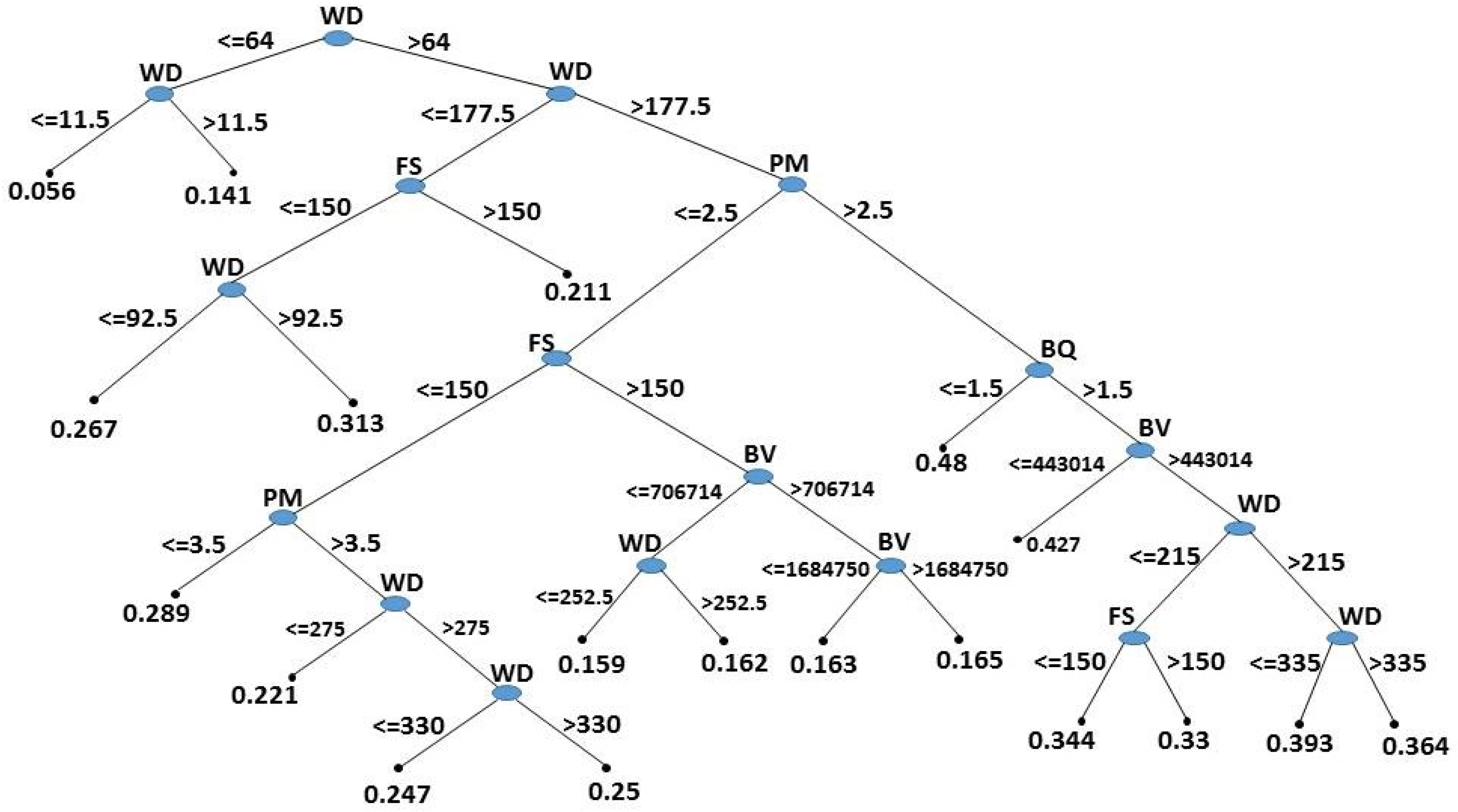
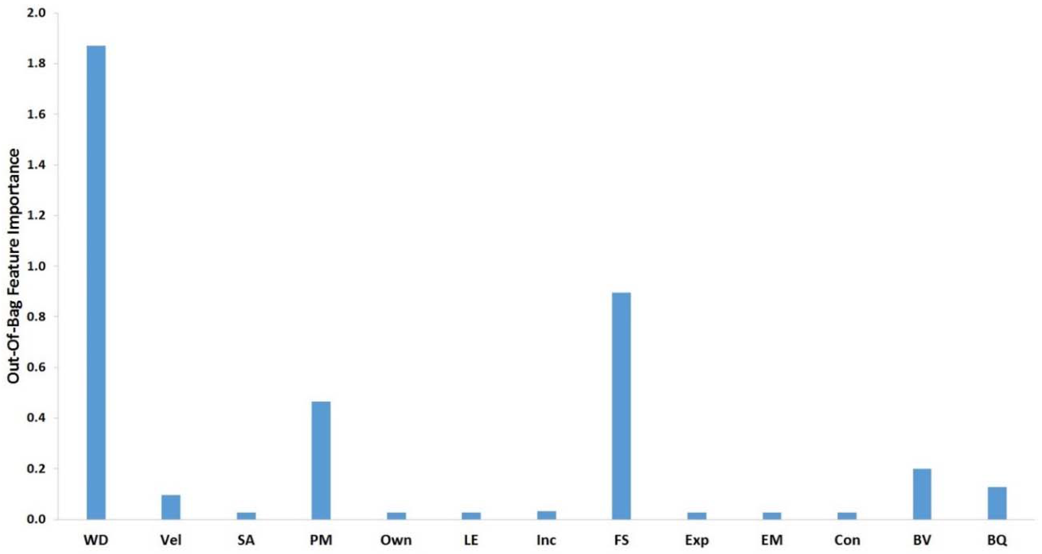
| Candidate Predictors | No. of Decision Nodes | Correlation with Loss Ratio |
|---|---|---|
| Water depth | 9 | + |
| Floor space | 3 | − |
| Precaution measures | 2 | − |
| Building value | 3 | N.A. |
| Building quality | 1 | − |
© 2016 by the authors; licensee MDPI, Basel, Switzerland. This article is an open access article distributed under the terms and conditions of the Creative Commons Attribution (CC-BY) license (http://creativecommons.org/licenses/by/4.0/).
Share and Cite
Hasanzadeh Nafari, R.; Ngo, T.; Mendis, P. An Assessment of the Effectiveness of Tree-Based Models for Multi-Variate Flood Damage Assessment in Australia. Water 2016, 8, 282. https://doi.org/10.3390/w8070282
Hasanzadeh Nafari R, Ngo T, Mendis P. An Assessment of the Effectiveness of Tree-Based Models for Multi-Variate Flood Damage Assessment in Australia. Water. 2016; 8(7):282. https://doi.org/10.3390/w8070282
Chicago/Turabian StyleHasanzadeh Nafari, Roozbeh, Tuan Ngo, and Priyan Mendis. 2016. "An Assessment of the Effectiveness of Tree-Based Models for Multi-Variate Flood Damage Assessment in Australia" Water 8, no. 7: 282. https://doi.org/10.3390/w8070282
APA StyleHasanzadeh Nafari, R., Ngo, T., & Mendis, P. (2016). An Assessment of the Effectiveness of Tree-Based Models for Multi-Variate Flood Damage Assessment in Australia. Water, 8(7), 282. https://doi.org/10.3390/w8070282