Frequency Analysis of High Flow Extremes in the Yingluoxia Watershed in Northwest China

Abstract

Statistical modeling of hydrological extremes is significant to the construction of hydraulic engineering. This paper, taking the Yingluoxia watershed as the study area, compares the annual maximum (AM) series and the peaks over a threshold (POT) series in order to study the hydrological extremes, examines the stationarity and independence assumptions for the two series, and discusses the estimations and uncertainties of return levels from the two series using the Generalized Extreme Value (GEV) and Generalized Pareto distribution (GPD) models. For comparison, the return levels from all threshold excesses with considering the extremal index are also estimated. For the POT series, the threshold is selected by examining the mean excess plot and the stability of the parameter estimates and by using common-sense. The serial correlation is reduced by filtering out a set of dependent threshold excesses. Results show that both series are approximately stationary and independent. The GEV model fits the AM series well and the GPD model fits the POT series well. The estimated return levels are fairly comparable for the AM series, the POT series, and all threshold excesses with considering the extremal index, with the difference being less than 10% for return periods longer than 10 years. The uncertainties of the estimated return levels are the highest for the AM series, and next for the POT series and then for all threshold excesses series in turn.

1. Introduction

A significant amount of attention has been paid to hydrological extreme events, which are likely to increase in frequency in most regions of the world [1,2,3]. There are two common ways to study the so called extreme events: one is the annual maximum series (AM) and the other is the peaks over a threshold (POT) series [4,5,6,7]. Rao and Hamed [8] showed that the AM series is statistically more efficient than the POT series when $\mathsf{\lambda }$ is small ( $\mathsf{\lambda }<1.65$ ), where $\text{ λ}$ is the mean number of peaks per year included in the POT series. However, as only the peak flow in each year is considered, the use of the AM series may involve some loss of information. For example, the second or third peak within a year may be greater than the maximum flow in other years, and yet they are ignored [6]. This situation is avoided in the POT series where all peaks above a certain threshold value are considered, and thus more information about the extremes would be involved in the analysis [6]. In the study of Madsen et al. [9], they found that the POT model is more advantageous than the AM model in cases where only short records are available. The POT series also has some obvious disadvantages, and the major one is that the flood peaks might not form an independent time series, since some flood peaks may occur on the recession curves of the preceding flood peaks [10]. Thus, both series are used to indicate high flow extremes and compared to each other in this study.

Plenty of probability distribution models, e.g., the Log Pearson Type III (LP3), Loglogistic, Lognormal, Burr, Weibull, Gamma, Generalized Extreme Value (GEV) model, and the Generalized Pareto distribution (GPD) are commonly used in fitting extreme events [11,12,13]. Rahmani et al. [14] used the Weibull distribution to calculate the extreme precipitation frequency in Kansas and its adjacent states. Du et al. [15] and Xia et al. [6] used the GEV and GPD models to estimate the historical extreme precipitation frequency in the Haihe and Huaihe river basins of China. Benyahya et al. [12] compared five probability distributions to identify the appropriate modes for providing the most accurate seasonal maximum precipitation in southern Quebec, Canada. Some studies show that the GEV or GPD model provides optimum fitness to extreme events for comparison studies [4,12,16], while others show different results [13,17].

Most of the extreme value models have been obtained through mathematical arguments that assume an underlying process consisting of a sequence of independent and stationary variables. However, for the types of data to which extreme value models are commonly applied, such assumptions are usually unrealistic [18]. Ling et al. [19] detected an abrupt change in 1993 in the high-flow index of the annual runoff for the Tarim River basin over the last 50 years. Chen et al. [20] found a change point in 1991 for the annual maximum flood flow in southern China. Although the usual extreme value models are still applicable in the presence of non-stationary and temporal dependence [18], the estimations of the model parameters and return levels based on model fitting would be suspicious without considering these assumptions [4,20,21,22,23]. Therefore, there is a need to investigate the validity of the stationarity and independence assumptions for the series before probability modeling is performed.

This study uses the AM and the POT series to indicate the hydrological extremes for the Yingluoxia watershed, and mainly focuses on the following issues: (1) the selection of the threshold for the POT series and a comparison of the AM and POT series; (2) statistical tests of the stationarity and independence assumptions for the AM series; and (3) estimations and uncertainties of the return levels for both series using the GEV and GPD models.

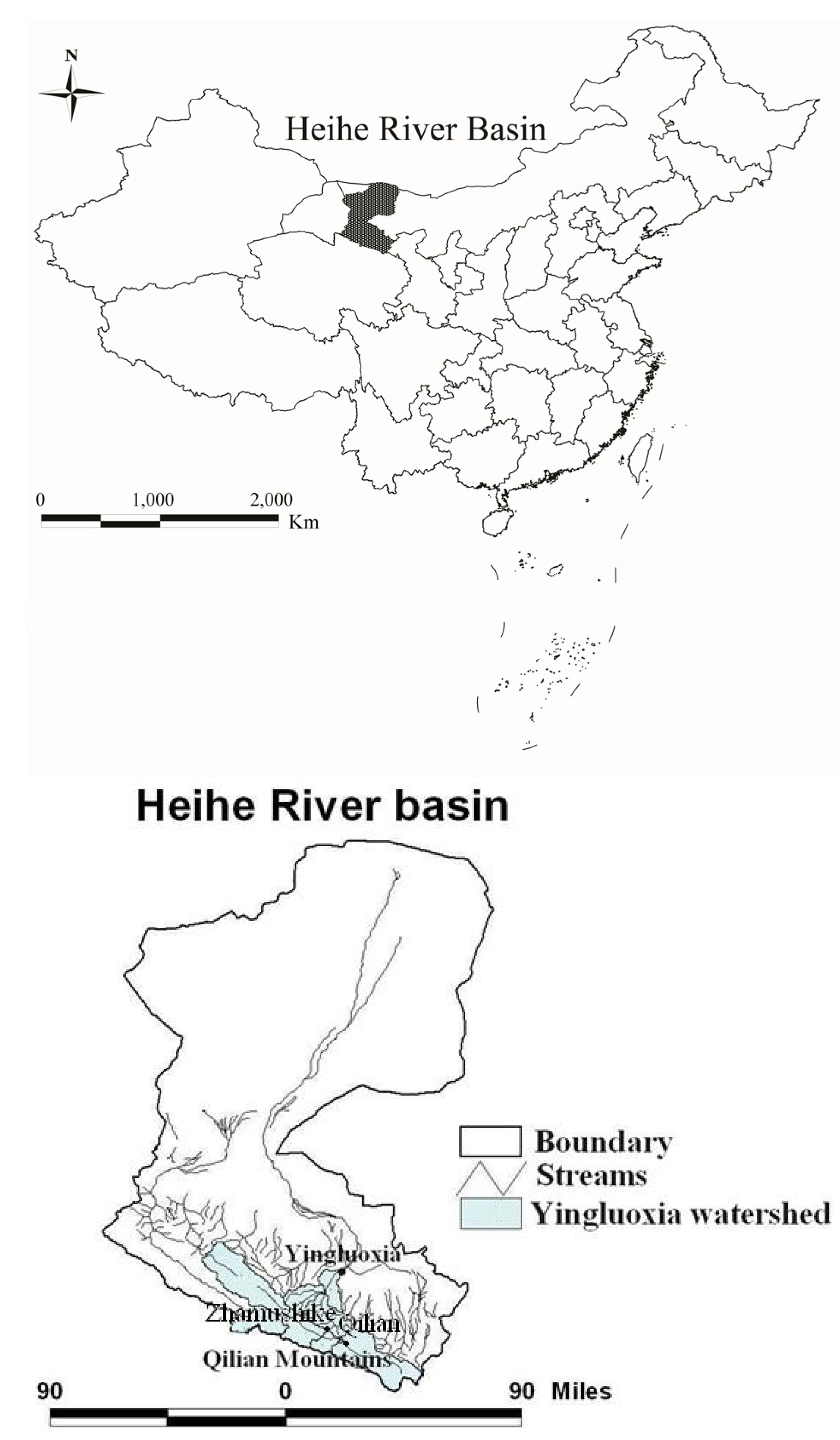
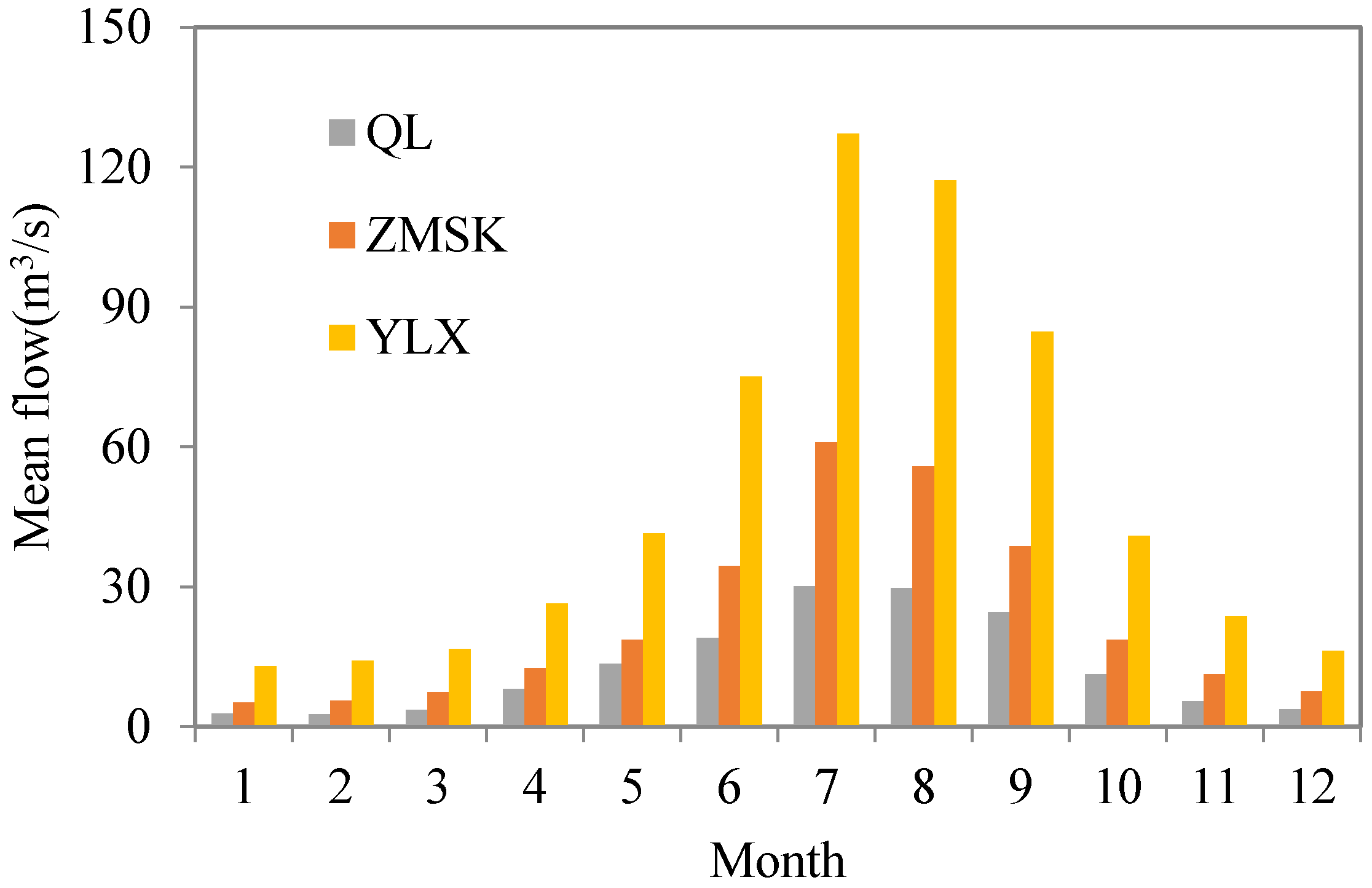
2. Study Area and Data Description

The Heihe River basin, the second largest inland river basin in China, has received a great deal of attention from the public and from water authorities. Based on the available literatures, most of the previous studies are mainly focused on the mean flows [24,25]. For better disaster management and mitigation in general, it is important to be aware that understanding the changes in flow extremes is more important than understanding the changes in the mean pattern [26].

The Heihe River basin, which originates from the Qilian Mountains, is located between 37° N–42° N latitude and 97° E–102° E longitude. The Yingluoxia watershed is the upper reach of the Heihe River basin (Figure 1). The area of this watershed reaches 10,009 km² and its altitude ranges from 3300 m asl to 1700 m asl. About 50% of the total runoff at the watershed outlet is generated in the mid-mountain zone (>2900 m asl) [27]. With the decreasing of altitude, the annual mean precipitation decreases from 400 mm to 180 mm, and the annual mean temperature increases from −3 °C to 7 °C. There are three hydrological stations in the watershed. The locations and the basic information for three stations are shown in Figure 1 and

Table 1. Basic information for three hydrological stations and their statistics on the annual flow in the Yingluoxia watershed.

Station Name (Abbreviation)	Longitude	Latitude	Elevation (m asl)	Data Period	Data Length	Annual Mean (m3/s)	Cv	Skewness
Qilian (QL)	100°15′ E	38°11′ N	2787	1967–2011	36	13.00	1.11	2.67
Zhamushike (ZMSK)	99°59′ E	38°14′ N	2810	1957–2011	48	23.16	1.16	3.52
Yingluoxia (YLX)	100°11′ E	38°49′ N	1700	1944–2011	66	51.64	1.07	3.21

Note: For QL station, the data for 1988–1989, 1992, 1997, and 2001–2005 are unavailable. For ZMSK station, the data for 1988–1989, and 2001–2005 are unavailable. For YLX station, the data for 1988–1989 are unavailable.

. The flow data of the 36-year, 48-year, and 66-year flow volumes for the stations are obtained from the National Hydrological Statistical Yearbook, and they are regularly checked and can be regarded to be of good quality. The annual mean flow is 13 m³/s, 23 m³/s, and 52 m³/s for QL, ZMSK, and YLX stations, respectively. As is shown by Figure 2, the inter-annual distributions of monthly flow are quite uneven, highly correlated with the temporal distributions of precipitation in the basin. Nearly 80% of precipitation is concentrated in June–September, with the largest frequencies concentrated in July. The annual maximum flow usually occurs in July or August.

3. Methodology Description

3.1. Probability Modeling

The probability distribution of the AM series can be statistically fitted by making use of the family of extreme value distributions referred to as the Generalized Extreme Value (GEV), which was introduced by Jenkinson [28]. GEV distribution has been widely used in the analysis of hydrological extremes because of its flexibility in representing three asymptotic types of extreme value probability distributions [4,16]. The cumulative probability function (CDF) for GEV distribution is given by:

$$F\left(x\right)=\text{exp}[-{\left(1+\mathsf{\xi }\frac{x-\mathsf{\mu }}{\mathsf{\sigma }}\right)}^{-\frac{1}{\mathsf{\xi }}}]\mathsf{\xi }\ne 0$$

(1)

where µ, $\mathsf{\sigma }$ and $\mathsf{\xi }$ are the location, scale and shape parameters, respectively. In the case $\mathsf{\xi }$ = 0, the distribution matches the Extreme Value type 1 (EV1) or Gumbel distribuon.

The POT series usually states that excesses from any sample over a high threshold may follow such distributions as exponential or Generalized Pareto distributions (GPD). Here, we choose the GPD to fit the POT series due to its flexibility in representing the different types of extreme value probability distributions. The theoretical development of the GPD can be found in Coles [18]. The CDF for the GPD distribution is given by:

$$G\left(x\right)=1-{\left(1+\mathsf{\xi }\frac{x-u}{{\mathsf{\sigma }}_u}\right)}^{-\frac{1}{\mathsf{\xi }}}\mathsf{\xi }\ne 0$$

(2)

where $u$ is the location parameter, also known as the threshold; x − $u$ is the series of exceedances over the threshold. ${\mathsf{\sigma }}_u$ and $\mathsf{\xi }$ are referred to as the scale and shape parameters, respectively. For a given shape parameter, the scale parameter controls the mean of the exceedances above the threshold. The value of $u$ must be specified before fitting Equation (2), since the GPD is a distribution of the threshold excesses [18]. The shape and scale parameters in GEV and GPD distributions are estimated by the maximum likelihood estimation (MLE) [29,30].

The Kolmogorov-Smirnov (K-S) test and the Anderson-Darling (A-D) test are performed for evaluating the suitability of selected probability distributions. Assume a random sample, $x_{1,\cdots }{x}_{\mathrm{n}}$ , from some distribution with CDF, F(x). The empirical CDF is F_n(x) = 0, i/N₀, 1 for x < x₁, x_i ≤ x and x ≤ x_i+1, x ≥ x_n, where $N_0$ is the number of observations. The statistic $D_{\text{max}}$ in the K-S test is defined as:

$$D_{\text{max}}={\text{max}}_{1\le \mathrm{i}\le N_0}\left[\mathrm{F}\left(x_{\mathrm{i}}\right)-\frac{\mathrm{i}-1}{N_0},\frac{\mathrm{i}}{N_0}-\mathrm{F}\left(x_{\mathrm{i}}\right)\right]$$

(3)

If $D_{\text{max}}>D_{\mathrm{n}}^{\mathsf{\alpha }}$ (the critical value at the significance level of α), then the null hypothesis that the data follows a specified distribution is rejected. The K-S test tends to be more sensitive near the center of the distribution, while the A-D test gives more weight to the tails. The Anderson-Darling statistic, $A^2$ , is defined as:

$$A^2=-N_0-{{\displaystyle \sum }}_{i=1}^n\frac{\left(2i-1\right)\left\{\text{ln}F\left(x_{\left(\mathrm{i}\right)}\right)+\text{ln}\left[1-F\left(x_{\left(n-i+1\right)}\right)\right]\right\}}{N_0}$$

(4)

where $x_{\left(1\right)},\cdots ,x_{\left(\mathrm{n}\right)}$ are the ordered observations, in an increasing order. If $A^2>A_{\mathsf{\alpha }}^2$ (the critical value at the significance level α), the hypothesis regarding the distributional form is rejected [31].

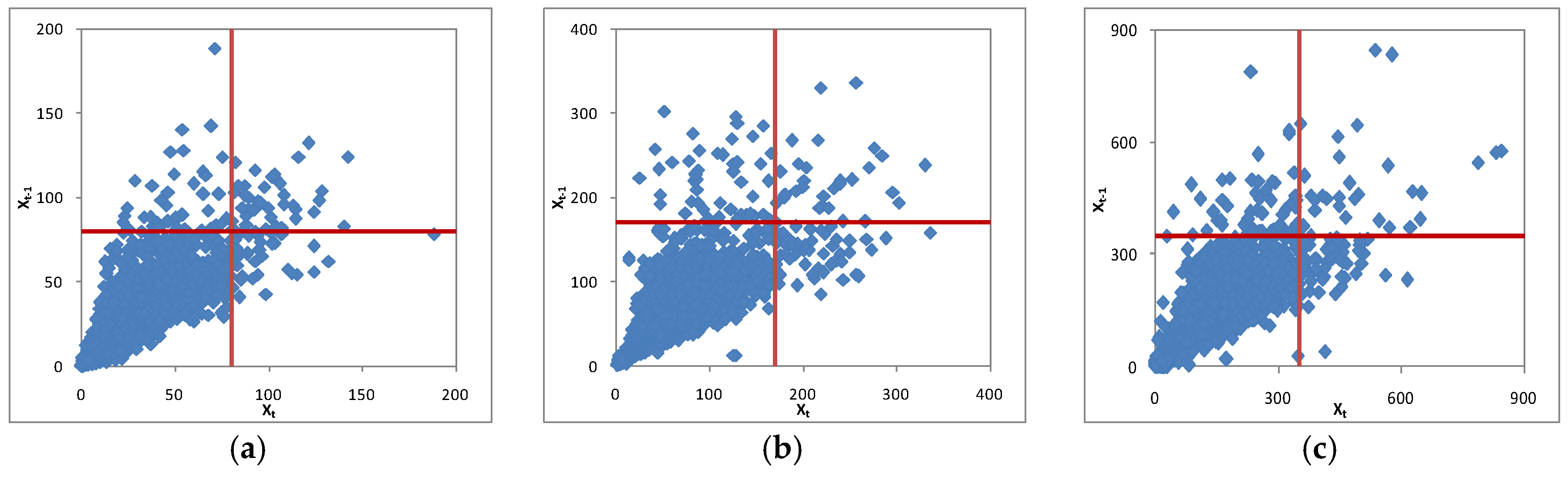
3.2. Stationarity and Independence Tests

We examine the stationarity and independence assumptions by estimating the features of the change points in mean, monotonic trends, and autocorrelations for the series. The presence of change-points can have a significant impact on the results of the monotonic trend analyses [20], and we first perform a change-point analysis. The Pettitt test [32], a non-parametric test based on a version of the Mann-Whitney statistic that allows testing whether two samples are from the same population, is used to test the high flow extremes data for abrupt changes in the mean. The test statistic, U_t,n, in the Pettitt test is given by:

$$U_{\mathrm{t},\mathrm{n}}=U_{\mathrm{t}-1}+{\displaystyle \sum }_j^n\text{sgn}(x_t-x_j)\left(t=2,3,\cdots ,n\right)$$

(5)

and $k\left(\mathrm{t}\right)={\text{max}}_{1\le t\le n}\left|U_{\mathrm{t},\mathrm{n}}\right|$ represents the most significant change point t. n means the data record length. If $k\left(\mathrm{t}\right)<\sqrt{-\frac{(n^3+n^2)\text{ln}\frac{\mathrm{p}}{2}}{6}}$ , then the null hypothesis of Pettitt’s test, with the absence of a changing point, will be accepted, at a specified significance level $p$ such as 0.05 (0 $<p<1$ ).

The presence of monotonic trends of time series are investigated by means of one of the most widely used tests, the Mann-Kendall test [33]. This test is non-parametric, making it more robust against outliers and departures from normality, which usually occurs in hydrological datasets. In the Mann-Kendall test $Z_{\mathrm{c}}$ is given by

$$\begin{gathered} Z_{\mathrm{c}}=\{\begin{array}{c}\frac{\mathrm{s}-1}{\sqrt{\text{var}\left(\mathrm{s}\right)}} \mathrm{s}>0\\ 0 \mathrm{s}=0\\ \frac{\mathrm{s}+1}{\sqrt{\text{var}\left(\mathrm{s}\right)}} \mathrm{s}<0\end{array} \\ s={\displaystyle \sum }_{i=1}^{n-1}{\displaystyle \sum }_{j=i+1}^n\text{sgn}(x_{\mathrm{j}}-x_{\mathrm{i}}) \end{gathered}$$

(6)

where $n$ is the data record length, and $x_{\mathrm{i}}$ and $x_{\mathrm{j}}$ are the sequential data values. When $\left|Z_{\mathrm{c}}\right|>{\mathrm{z}}_{1-\mathsf{\alpha }/2}$ , in which ${\mathrm{z}}_{1-\mathsf{\alpha }/2}$ are the standard normal deviates and α is the significance level, H₀ (no significant trend in dataset) will be rejected. Q, the gradient of Kendall, shows the extent of trends. It means an upward trend when Q is positive and a downward trend when it is negative, where $Q=\text{Median}\left(\frac{x_{\mathrm{j}}-x_{\mathrm{i}}}{j-\mathrm{i}}\right)$ ( $1<i<j<n$ ).

We employ the autocorrelation test by examining the autocorrelation coefficients to check the assumption of independence for the data series. When the absolute values of the autocorrelation coefficients of different lag times, for a time series with n observations, are not larger than the typical critical value, i.e., $1.96/\sqrt{n}$ corresponding to the 0.05 significance level, the observations in the time series can be regarded as being independent from each other.

3.3. Return Level Estimations

When we explore the extreme events, what extreme events might occur on 100-year or even longer return periods given the much shorter period data available is another active topic [5,22]. Suppose that a GEV with parameters μ, ξ and σ is a suitable model for the AM series, the estimations of high flow extremes, x, at a given return period, T, can be obtained from

$$x=\mathsf{\mu }-\frac{\mathsf{\sigma }}{\mathsf{\xi }}\left[1-{\left(-\ln \left(1-\frac{1}{T}\right)\right)}^{-\mathsf{\xi }}\right]\mathsf{\xi }\ne 0$$

(7)

Suppose that a GDP with parameters ξ and σ_u is a suitable model for the exceedances of a threshold, u. The estimations of high flow extremes x_m, which is exceeded on average once every $\text{ m }$ observations, can be written as:

$$x_{\text{m}}=u+\frac{{\text{σ}}_u}{\mathsf{\xi }}[\left({\mathsf{\zeta }}_{\text{u}}{)}^{\mathsf{\xi }}-1\right]\mathsf{\xi }\ne 0$$

(8)

in which ${\mathsf{\zeta }}_{\mathrm{u}}=\frac{k}{n}$, k is the exceedance data length (for example, k = 32 for QL station shown in

Table 2. Statistics of the AM and POT series for the three stations in the Yingluoxia watershed.

Station	AM				POT
	Sample Size	Maximum (m3/s)	Minimum (m3/s)	Mean (m3/s)	Threshold (m3/s)	Sample Size	Minimum (m3/s)	Mean (m3/s)
QL	36	188 (1974)	47 (1994)	97	80	32	81 (1990)	109
ZMSK	48	336 (1960)	87 (1985)	205	170	45	171 (1961, 1986, 2009)	228
YLX	66	845 (1952)	166 (1973)	384	350	45	351 (1981)	467

Note: The year shown in the bracket is when maximum and minimum flows occurred.

) and n is the total observations in day (n = 36 × 365 = 13140 for QL station). For the POT series, the return period represents the average interval between the high flows that exceed threshold value, and thus the m-observation return level, x_m, is constructed. It is should be noted that there is an important distinction in meaning between the return periods computed from the AM and POT series. In the AM series, the return period is the average interval, in which a flood of a given size will occur as an annual maximum; while in the POT series, the return period represents the average interval between floods of a given size, regardless of their relation to the year or any other period [34]. It is often more convenient to give return levels on an annual scale, so that the T-year return level is approximately the level expected to be exceed once every T years. If there are N_y observations per year, this corresponds to the m-observation return level, where m = T × N_y [18]. The flow data is daily in this study, so the T-year return level corresponds to the m-observation return level with m = 365 × T. In this case, we finally get the return levels at a T-year return period instead of at an m-observation return period.

4. Results and Discussion

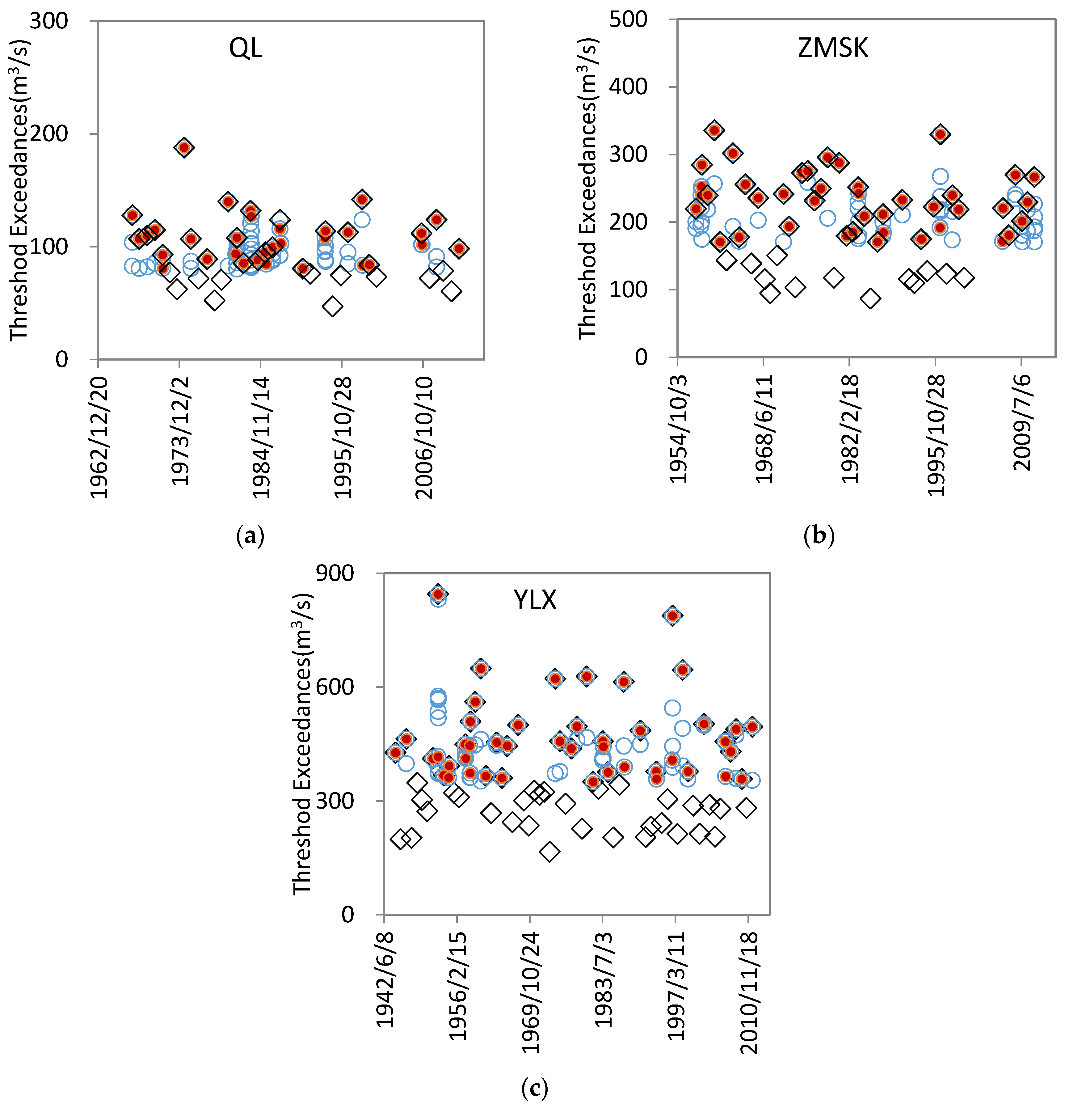
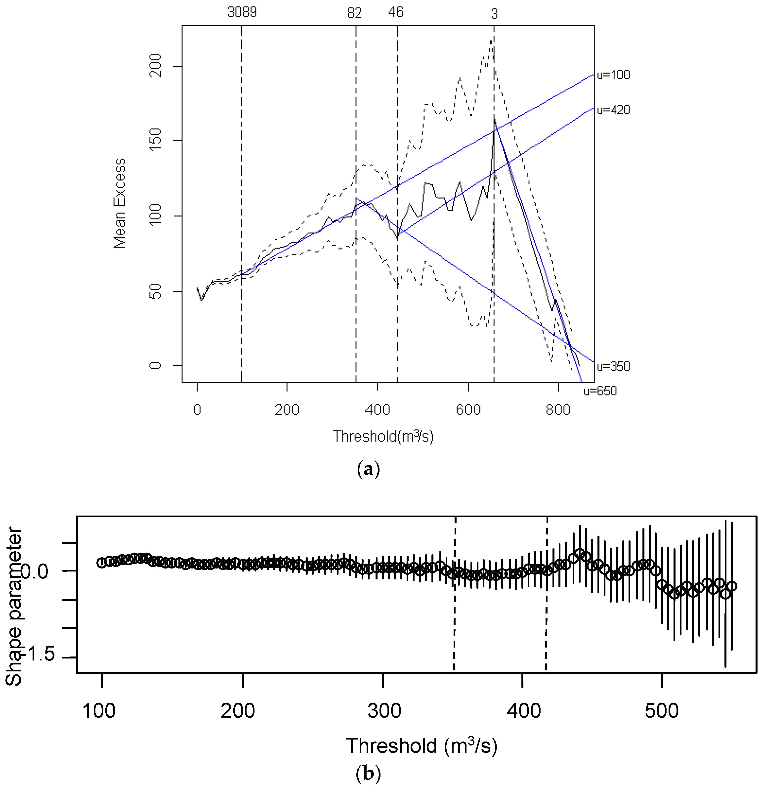
4.1. Threshold Selection and POT Series

Threshold selection for the POT series is not an easy task. Too low a threshold value is likely to violate the asymptotic basis of the model, leading to bias, while too high a threshold value will generate a few excesses, with which the model can be estimated, leading to high variance [18]. Scarrott and MacDonald [35] provided a comprehensive review of threshold selection approaches. In this article, combined with the consideration of the physical meanings of “high flow extremes”, we mainly employ two commonly used methods for the selection of the optimum threshold [5,36,37]: one is examining the mean excess plot carried out prior to model estimation, and the other is assessing the stability of parameter estimates based on model fittings across a range of different thresholds.

The mean excess plot uses the expectation of GPD excesses, E(X − u|X > u = σ_µ/(1 − ξ), as a diagnostic, defined for ξ <1 to ensure the mean exists. For any higher x > u, the expectation becomes $\mathrm{E}\left(X-x|X>x\right)=\left({\mathsf{\sigma }}_u+\mathsf{\xi }x\right)/\left(1-\mathsf{\xi }\right)$ , which is linear in x with gradient $\mathsf{\xi }/\left(1-\mathsf{\xi }\right)$ and intercept ${\text{ σ}}_u/\left(1-\mathsf{\xi }\right)$ . Empirical estimates of the sample mean excesses are typically plotted against a range of thresholds. The threshold is chosen to be the lowest level where all the higher threshold based sample mean excesses are consistent with a straight line [35]. Figure 3a presents the mean excess plot with 95% confidence intervals (CIs) for the daily flow data at YLX station, from the extRemes package in R. It is noted that the 95% CIs in Figure 3 are not quite right since this figure is based on the threshold exceedance data, not the POT data series. From Figure 3a, four fitted mean excess straight lines are detected corresponding to thresholds of 100 m³/s, 350 m³/s, 420 m³/s, and 650 m³/s. The threshold of 100 m³/s gives 3089 exceedances, corresponding to as many as 47 high flow extremes occurring per year on average during the period from 1944 to 2011, which deviates from the common cognition on extreme events. Above 650 m³/s, less than three exceedances are included, which are too few data points to make meaningful and reliable inferences. For thresholds of 350 and 420 m³/s, both mean excesses are presented as straight lines. While, there are relatively larger deviations from the fitted plot, and greater uncertainties on the estimated return levels for the threshold of 420 m³/s. Figure 3b shows the estimated shape parameter stability plot across threshold values ranging from 100 to >500 m³/s. The shape parameter should be constant above some threshold levels, where asymptotics begin to apply [16]. From Figure 3b, we find approximately constant estimates for the shape parameter above the threshold of 350 m³/s, and a very obvious decreasing or increasing trend is presented for the parameter estimates after the threshold of 420 m³/s, together with wider 95% CIs. Considering the points mentioned above, the threshold of 350 m³/s, yielding a threshold exceedance with 82 data, is finally identified for YLX station. Similar procedures are performed for QL and ZMSK stations, and thresholds of 80 m³/s and 170 m³/s are finally identified for the two stations. This assessment is largely subjective. Northrop and Coleman [38] and Wadsworth [39] reduce this subjectivity using a likelihood-based procedure to produce complementary plots that enable an automated threshold selection.

Figure 4 shows the daily flow time series against series at Lag 1 for the three stations, and the red lines in the plots represent the thresholds. Above the threshold, a short-term serial correlation (although it is not strong) seems to exist, indicating the presence of extremal dependence. There are two commonly used ways to deal with this problem. One is filtering out a set of approximately dependent threshold excesses, and another is estimating the extremal index [22]. We use the first approach to obtain an independent series. Considering the specific climatic and geographic conditions in one region, there is a criterion in the threshold exceedance series to meet the independence condition, and the successive high flow extremes should be separated by at least as many days as five plus the natural logarithm of the square miles in the basin area [40]. The three hydrological stations in the study area control basin areas of 3000–10,009 km², so the successive high flow extremes should be separated by at least as 12–13 days. Only the maximum flow is retained if successive high flow extremes occurred within the 12–13 days interval, and the rest are filtered out. We then get the POT series from the above declustering scheme with sample sizes of 32, 45, and 45 for QL, ZMSK, and YLX stations, respectively. Figure 5 shows the threshold exceedance series and the POT series. From Figure 5, no obvious trends or serial correlations are found for the POT series, which means that the POT series can be regarded as approximately independent and stationary from graphic diagnosis.

4.2. AM Series and Stationarity and Independence Tests

The AM series can be directly derived from the historical flow records, which consists of the maximum flow from each recorded year. The samples of the AM and POT series for the three stations are shown in Figure 5. The statistics of these two series are listed in Table 2. It is apparent that the numbers of high flow extremes in the POT series are not consistent with those in the AM series. For example, 31 out of 66 extremes in the AM series are not included in the POT series for YLX station, while lots of the second and even the third largest extremes from some years are included in addition to the largest one. The means of the POT series are 10%–18% higher than those of the AM series, which suggests that the POT series does take more extreme information into account in this study.

The results of stationarity and independence tests for the AM series are shown in

Table 3. Results of the stationarity and independence tests for the AM series in the Yingluoxia watershed.

Station	Change Point		Trend		Independence Test
	$k\left(t\right)$	Critical Value (P = 0.05)	$Z_c$	Q	Lag 1	Critical Value(α = 0.05)
QL	69	171.7	−1.10	−0.05	−0.08	0.33
ZMSK	119	263.5	−0.45	−0.39	−0.05	0.28
YLX	139	423.6	−0.23	−0.25	−0.11	0.24

. The calculated $k\left(\mathrm{t}\right)$ values in the Pettitt test are 69, 119, and 139 for QL, ZMSK, and YLX stations, respectively. These values are smaller than those of the critical values at the 0.05 significance level, which means that the null hypothesis, with the absence of a change point, will be accepted. Since no statistically significant change points are detected, we perform a monotonic trend analysis on the entire record of the AM series directly. The absolute values of test $Z_{\mathrm{c}}$ , in the Mann-Kendall test are smaller than the value of the normal standard deviations, $z_{1-\mathsf{\alpha }/2}$ (1.96 at $\mathsf{\alpha }=0.05$ ), which means that no significant trends are detected for the AM series at the 0.05 significance level. From the autocorrelation coefficients for Lag1 and their corresponding 95% CIs, the AM series for the three stations are not highly autocorrelated and do not violate the assumptions of independence. The above analysis suggests that the independence and stationarity assumptions are approximately satisfied for the AM series, i.e., the subsequent model fitting is straightforward, without requiring consideration of serial dependence or the parameter changes in probability models through time.

4.3. Frequency Analysis for High Flow Extremes

4.3.1. Probability Modeling

We fit the AM series using the GEV model and fit the POT series using the GPD model. The results of goodness-of-fit, together with the estimated optimal parameter values and standard errors (in the brackets), are shown in

Table 4. Goodness-of-fit of probability modeling and the parameter estimations and standard errors (given in the parentheses) for the GEV and GPD models for the three stations in the Yingluoxia watershed.

Station	K-S		A-D		Parameter Estimation
	$D_{\max }$	$D_n^{\alpha }$	$A^2$	$A_{\alpha }^{2 }$	$\mathsf{\mu }$	$\mathsf{\sigma }$	$\mathsf{\xi }$
AM-GEV
QL	0.09	0.22	0.19	2.50	84.76 (4.4943)	24.1494 (3.1982)	−0.0694 (0.1126)
ZMSK	0.08	0.20	0.33	2.50	183.48 (10.6038)	65.6735 (7.8552)	−0.3364 (0.1094)
YLX	0.06	0.16	0.26	2.50	316.48 (15.4693)	108.1400 (11.6639)	0.0436 (0.1116)
POT-GPD
QL	0.10	0.24	0.34	2.50	–	33.9589 (7.3896)	−0.2107 (0.1322)
ZMSK	0.08	0.20	0.42	2.50	–	86.9987 (16.6579)	−0.4716 (0.1392)
YLX	0.08	0.20	0.33	2.50	–	125.4130 (26.9464)	−0.0702 (0.1551)

Note: The significance level, $\mathsf{\alpha },$ is 0.05.

. The values of the estimated statistic, $D_{\text{max}}$ , in the K-S test are 0.09, 0.08, and 0.06 at QL, ZMSK, and YLX stations for the AM series, which is smaller than the critical values of $D_{\mathrm{n}}^{\mathsf{\alpha }}$ (0.22, 0.20, and 0.16 at the 0.05 significance level). The values of the estimated statistic, $A^2$ , in the A-D test are 0.19, 0.33, and 0.26 at the three stations for the AM series, which is smaller than the critical values of $A_{\mathsf{\alpha }}^2$ at the 0.05 significance level. As for the POT series, both the estimated statistic $D_{\text{max}}$ in the K-S test and the estimated statistic $A^2$ in the A-D test are smaller than the critical values of $D_{\mathrm{n}}^{\mathsf{\alpha }}\text{ and }{A}_{\mathsf{\alpha }}^2$ as well. It means that the GEV model fits the AM series well and the GPD model fits the POT series well.

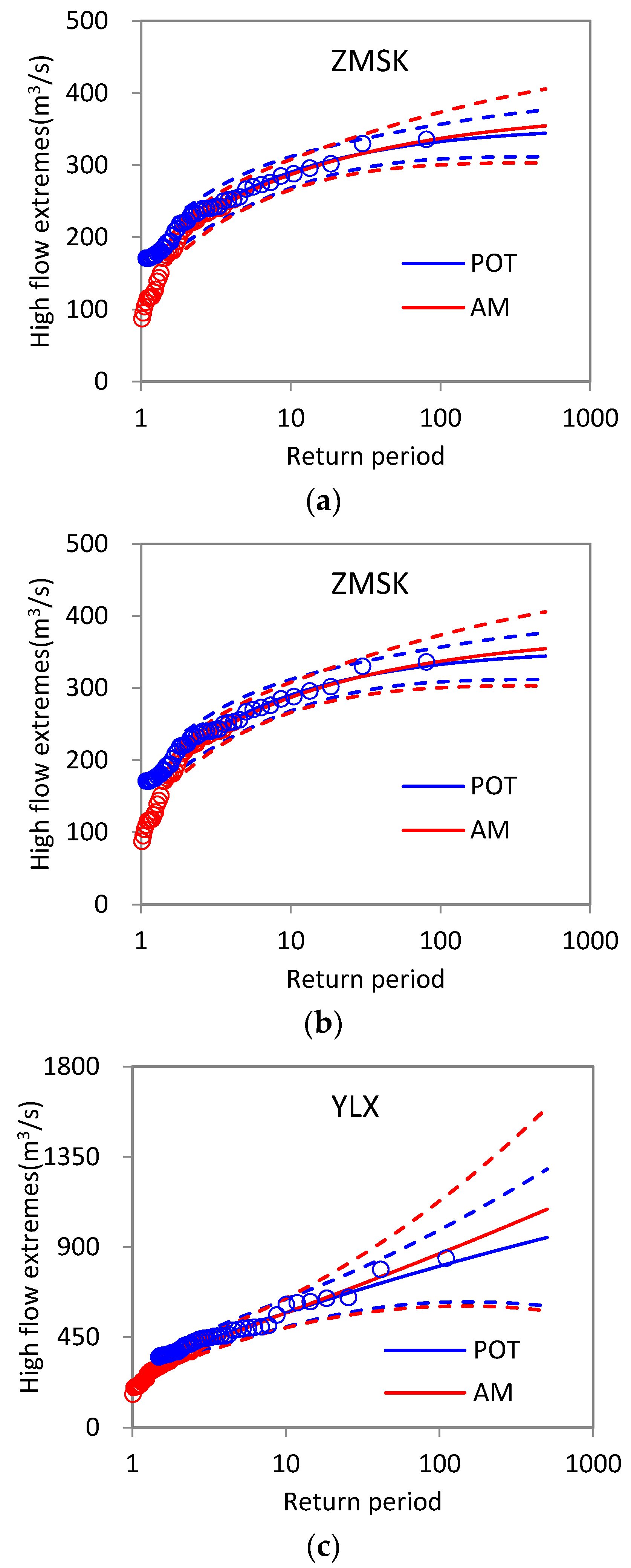
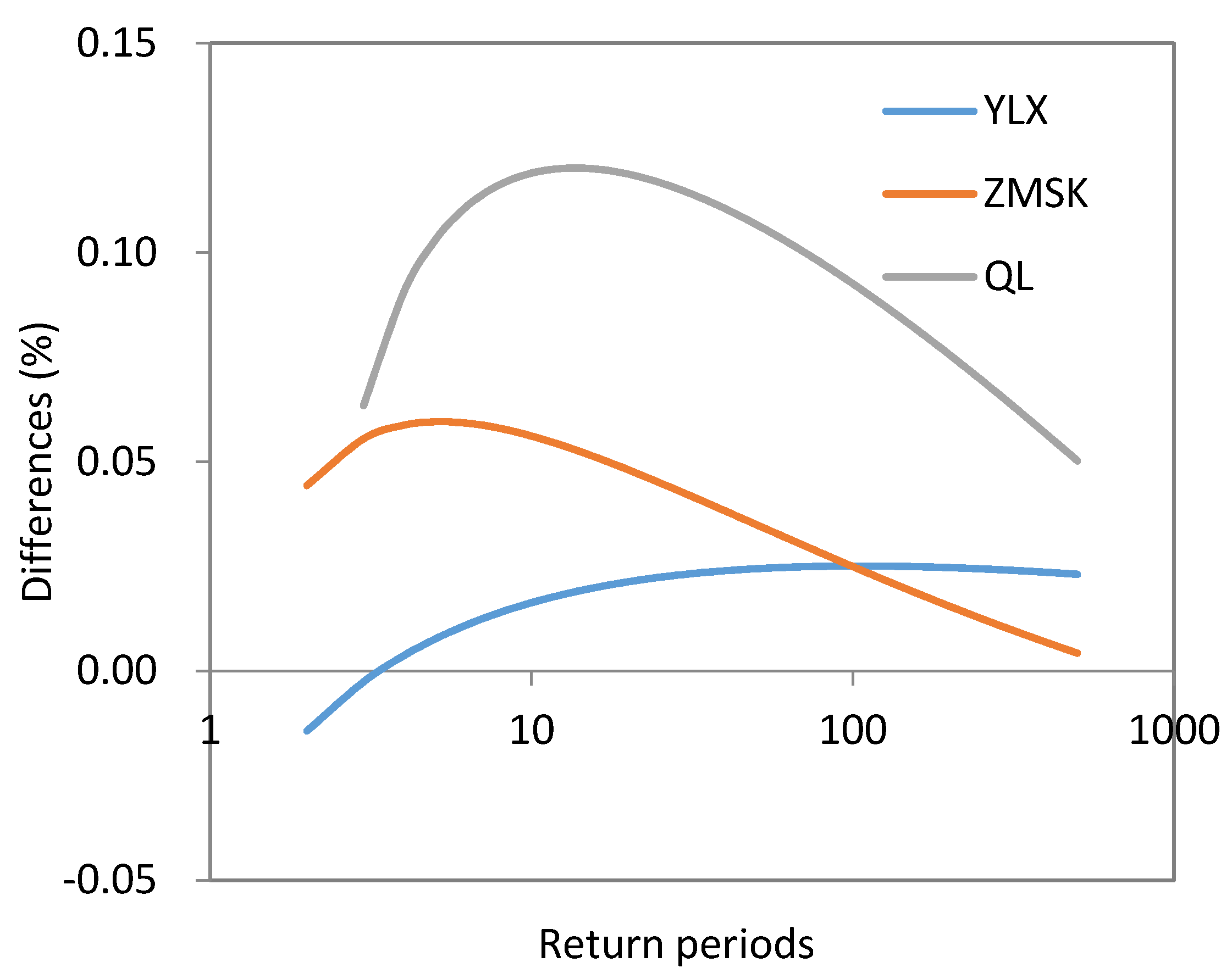
4.3.2. Return Level Estimation

Extremes are scarce, thus estimates are often required for levels of a process that are much greater than have already been observed. Estimates of daily high flow extremes at a given return period are essential for the local flooding protection; thus, different return levels of daily high flow extremes in the Yingluoxia watershed are estimated herein.

The estimated return levels (solid lines) and the corresponding 95% CIs (dashed lines) from both the AM and POT series are presented in Figure 6, together with the empirical return periods (red and blue circles). The empirical return periods for the AM series are calculated using $T=\frac{1}{1-\frac{\mathrm{i}-0.4}{\mathrm{k}+0.2}}$ in which i indicates the order of the ascending high flow extremes data (i = 1, 2,…, k), and k is the high flow data length [41]. The empirical return periods for the POT series are calculated using $T=\frac{1}{365\times {\mathsf{\zeta }}_{\mathrm{u}}\times \left(1-\frac{i-0.4}{k+0.2}\right)}$ , in which ${\mathsf{\zeta }}_{\mathrm{u}}=\frac{k}{n}$, k is the exceedence data length, n is the total observations in day, and i is the order of the ascending exceedance data (i = 1, 2,…, k). The GEV model provides a good match to the empirical estimations for the AM series and the GPD model provides a good match to those for the POT series.

Table 5. Estimations and 95% CIs (in the brackets) of return levels from the AM and the POT series for the Yingluoxia watershed, together with the differences of return level estimations from both series.

Station	T = 10	T = 50	T = 100	T = 200
AM_GEV (m3/s)
QL	135 (118,152)	167 (135,200)	180 (137,222)	192 (138,245)
ZMSK	287 (266,308)	326 (296,356)	337 (300,374)	346 (303,389)
YLX	572 (498,646)	776 (589,964)	867 (604,1131)	956 (604,1308)
POT_GPD (m3/s)
QL	143 (125,162)	169 (144,194)	179 (148,209)	187 (150,224)
ZMSK	295 (274,316)	325 (303,346)	333 (308,357)	339 (311,367)
YLX	591 (519,664)	743 (609,877)	807 (625,989)	869 (626,1112)
Difference (%)
QL	5.59	1.18	−0.56	−2.67
ZMSK	2.71	−0.31	−1.20	−2.06
YLX	3.21	−4.44	−7.43	−10.00

lists the estimated return levels for the AM and POT series from both the GEV and GPD models, together with the 95% CIs. These estimated return levels are expected to be helpful in providing useful information for the design of local flooding defenses. At the 10-year return period, the GEV model fitted values are 135 (8.45) m³/s, 287 (10.70) m³/s, and 572 (37.63) m³/s for QL, ZMSK, and YLX stations, and the GPD model fitted values are 143 (9.18) m³/s, 295 (10.71) m³/s, and 591 (37.17) m³/s for the three stations with standard errors given in the parentheses. At the 100-year return period, the fitted values increase to 180 (21.67) m³/s, 337 (18.64) m³/s, and 867 (134.18) m³/s for the GEV model, and 179 (15.82) m³/s, 333 (12.76) m³/s, and 807 (93.01) m³/s for the GPD model for the three stations. Overall, the results for the estimated return levels from both the GEV and GPD models are fairly comparable, with the largest difference being less than 10% for the 10-year, 20-year, 50-year, and 100-year return periods. However, the 95% CIs of the estimated return levels for the AM series based on the GEV model are wider than those for the POT series based on the GPD model (Figure 6) especially at the longer return periods, which means that greater uncertainties exist for the extrapolation from the AM series and GEV model.

The POT series makes use of more information on extremes than the AM series, though discarding all but the cluster maxima is still wasteful of data. For comparison, we attempt to use all threshold exceedance points to estimate the return levels of high flow extremes with considering the extremal index. In Fawcett and Walshaw [22], the authors proposed five extremal index estimators. Due to our practical experiences, we select the approach mentioned in Coles [18] to estimate the extremal index, i.e., the extremal index $\mathsf{\theta }=\frac{n_c}{n_u}$ , in which $n_{\mathrm{c}}$ indicates the number of clusters obtained above the threshold, and $n_u$ indicates the number of exceedances of the threshold. The m-observation return level is $x_{\mathrm{m}}=u+\frac{{\mathsf{\sigma }}_u}{\mathsf{\xi }}[\left({\mathsf{\zeta }}_u\mathsf{\theta }{)}^{\mathsf{\xi }}-1\right]$ ($\mathsf{\xi }\ne 0$), in which ${\mathsf{\zeta }}_u=\frac{n_u}{n}$ [18], and the meanings of $u$ , ${\mathsf{\sigma }}_{\mu }$ , and $\mathsf{\xi }$ are the same as those in Equation (8).

Figure 7 shows the differences between the two schemes on the estimated return level. The differences are calculated with the formula of relative error. From Figure 7, the differences are not great between the POT series and all the threshold exceedances with considering the extremal index for the estimated return levels. For YLX station, it is relatively stable and within 3%. For ZMSK station, it is about 6% at less than 10-year return periods and decreases to lower than 5% with the return periods increasing. For QL station, relatively larger differences are found, with 10%–12% differences for less than 10-year return periods and 5%–10% differences for the longer return periods. These two schemes give close results in return level estimations especially for YLX and ZMSK stations. We further analyze the 95% CIs of the estimated return levels from the two schemes. Results are shown in

Table 6. Estimations and 95% CIs (in the brackets) of return levels from the threshold exceedances with considering the extremal index for the Yingluoxia watershed.

Station	T = 10	T = 50	T = 100	T = 200
QL	126 (111,141)	151 (126,175)	162 (133,192)	173 (137,209)
ZMSK	279 (262,297)	314 (294,333)	325 (302,347)	334 (306,361)
YLX	581 (515,647)	725 (598, 851)	787 (619, 954)	847 (631,1063)

. The 95% CIs from the threshold exceedances are slightly narrower than those from the POT series. For example, for YLX station, the standard errors of the estimated return levels from the threshold exceedances are 33.55, 64.43, 85.45, and 110.25 at the 10-year, 50-year, 100-year, and 200-year return periods, which are lower than those from the POT series with 37.17, 68.28, 93.01, and 123.74, respectively. Due to more data being involved in the analysis, using all excesses with considering the extremal index will tend to give more accurate return level estimates than those from the POT series. This result is consistent with the findings of Fawcett and Walshaw [22].

Note that for the extremal index used here, there are other methods possible for estimating the extremal index. Return level estimations are sensitive to the choice of the estimator of the extremal index, and extremal index values are related to the strength of serial correlation in the threshold exceedance series. Fawcett and Walshaw [22] have attempted to discuss this issue and found many meaningful results. As this paper mainly discusses the AM and POT series and probability modeling using the GEV and GPD models, we will pursue further research into this area by considering other estimation approaches for the extremal index, which would be helpful in understanding how the extremal index estimators affect the estimations and uncertainties of the return levels.

5. Conclusions

Both the AM and POT series are commonly used to study extreme events. In this paper, we construct these two series to indicate the hydrological extremes in the Yingluoxia watershed, and compare the estimations and uncertainties of return levels for both series by using the GEV and GPD models. Using all threshold excesses with considering the extremal index to estimate the return levels is also investigated for comparison. Before the probability modeling, the stationarity and independence assumptions for the AM and POT series are examined since ignoring these assumptions would result in errors in the estimations of the model parameters and return levels based on model fitting. Results show that, combined with a declustering scheme, the POT series are approximately independent, and they are also broadly stationary based on the graphic diagnosis. The AM series can be regarded as stationary and independent with the results of Mann-Kendall test, Pettitt test, and autocorrelation coefficient test. The GEV model fits the AM series well, and the GPD model fits the POT series well according the statistical K-S test and A-D test. The estimated return levels from the AM series, the POT series, and all threshold exceedances with considering the extremal index are fairly comparable. The largest difference between the former two series is less than 10% at the 10-year, 20-year, 50-year, and 100-year return periods. The difference between the latter two series increases first and then decreases as the return period increasing, and it is less than 10% for return periods over 10 years. As for the uncertainties of the estimated return levels, the AM series show the largest uncertainties on extrapolation, followed by the POT series. The threshold excesses with considering the extremal index tend to show the smallest uncertainties of return level estimations with the narrowest 95% CIs, due to more data involved in the analysis.

References

1. Dahlke, H.E.; Lyon, S.W.; Stedinger, J.R.; Jansson, P. Contrasting trends in floods for two sub-arctic catchments in northern Sweden—Does glacier presence matter? Hydrol. Earth Syst. Sci. 2012, 16, 2123–2141. [Google Scholar] [CrossRef]
2. Kay, A.L.; Jones, D.A. Transient changes in flood frequency and timing in Britain under potential projections of climate change. Int. J. Climatol. 2012, 32, 489–502. [Google Scholar] [CrossRef] [Green Version]
3. Jha, M.K.; Singh, A.K. Trend analysis of extreme runoff events in major river basins of Peninsular Malaysia. Int. J. Water 2013, 7, 142–158. [Google Scholar] [CrossRef]
4. Villarini, G.; Smith, J.A.; Baeck, M.L.; Vitolo, R.; Stephenson, D.B.; Krajewski, W.F. On the frequency of heavy rainfall for the Midwest of the United States. J. Hydrol. 2011, 400, 103–120. [Google Scholar] [CrossRef]
5. Du, H.; Xia, J.; Zeng, S.D.; She, D.X.; Zhang, Y.Y.; Yan, Z.Q. Temporal and spatial variations and statistical models of extreme runoff in Huaihe River Basin. Acta Geogr. Sin. 2012, 67, 398–409. (In Chinese) [Google Scholar]
6. Xia, J.; Du, H.; Zeng, S.; She, D.; Zhang, Y.; Yan, Z.; Ye, Y. Temporal and spatial variations and statistical models of extreme runoff in Huaihe River basin during 1956–2010. J. Geogr. Sci. 2012, 22, 1045–1060. [Google Scholar] [CrossRef]
7. Asl, S.J.; Khorshiddoust, A.M.; Dinpashoh, Y.; Sarafrouzeh, F. Frequency analysis of climate extreme events in Zanjan, Iran. Stoch. Environ. Res. Risk Assess. 2013, 27, 1637–1650. [Google Scholar]
8. Rao, A.R.; Hamed, K.H. Flood frequency Analysis; CRC Press LLC: New York, NY, USA, 1999. [Google Scholar]
9. Madsen, H.; Rasmussen, P.F.; Rosbjerg, D. Comparison of annual maximum series and partial duration series methods for modeling extreme hydrologic events. Water Resour. Res. 1997, 33, 747–757. [Google Scholar] [CrossRef]
10. Bezak, N.; Brilly, M.; Šraj, M. Comparison between the peaks-over-threshold method and the annual maximum method for flood frequency analysis. Hydrol. Sci. J. 2014, 59, 959–977. [Google Scholar] [CrossRef]
11. Rahman, A.S.; Rahman, A.; Zaman, M.A.; Haddad, K.; Ahsan, A.; Imteaz, M. A study on selection of probability distributions for at-site flood frequency analysis in Australia. Nat. Hazards 2013, 69, 1803–1813. [Google Scholar] [CrossRef]
12. Benyahya, L.; Gachon, P.; St-Hilaire, A.; Laprise, R. Frequency analysis of seasonal extreme precipitation in sounthern Quebec (Canada): An evaluation of regional climate model simulation with respect to two gridded datasets. Hydrol. Res. 2014, 45, 115–133. [Google Scholar] [CrossRef]
13. Li, Z.; Brissette, F.; Chen, J. Assessing the applicability of six precipitation probability distribution models on the Loess Plateau of China. Int. J. Climatol. 2014, 34, 462–471. [Google Scholar] [CrossRef]
14. Rahmani, V.; Hutchinson, S.L.; Hutchinson, J.M.S.; Anandhi, A. Extreme daily rainfall event distribution patterns in Kansas. J. Hydrol. Eng. 2014, 19, 707–716. [Google Scholar] [CrossRef]
15. Du, H.; Xia, J.; Zeng, S.; She, D.; Liu, J. Variations and statistical probability characteristic analysis of extreme precipitation events under climate change in Haihe River Basin, China. Hydrol. Process. 2014, 28, 913–925. [Google Scholar] [CrossRef]
16. Shamir, E.; Georgakakos, K.P.; Murphy, M.J. Frequency analysis of the 7–8 December 2010 extreme precipitation in the Panama Canal watershed. J. Hydrol. 2013, 480, 136–148. [Google Scholar] [CrossRef]
17. Papalexiou, S.M.; Koutsoyiannis, D.; Makropoulos, C. How extreme is extreme? An assessment of daily rainfall distribution tails. Hydrol. Earth Syst. Sci. 2013, 17, 851–862. [Google Scholar] [CrossRef]
18. Coles, S. An Introduction to Statistical Modeling of Extreme Values; Springer: London, UK, 2001. [Google Scholar]
19. Ling, H.B.; Xu, H.L.; Fu, J.Y. High- and low-flow variations in annual runoff and their response to climate change in the headstreams of the Tarim River, Xinjiang, China. Hydrol. Process. 2013, 27, 975–988. [Google Scholar] [CrossRef]
20. Chen, X.H.; Zhang, L.J.; Xu, C.Y.; Zhang, J.M.; Ye, C.Q. Hydrological design of nonstationary flood extremes and durations in Wujiang river, South China: changing properties, causes and impacts. Math. Probl. Eng. 2013, 2013, 1–10. [Google Scholar] [CrossRef]
21. Fawcett, L.; Walshaw, D. Improved estimation for temporally clustered extremes. Environmetrics 2007, 18, 173–188. [Google Scholar] [CrossRef]
22. Fawcett, L.; Walshaw, D. Estimating return levels from serially dependent extremes. Environmetrics 2012, 23, 272–283. [Google Scholar] [CrossRef]
23. Yang, T.; Shao, Q.X.; Hao, Z.C.; Chen, X.; Zhang, Z.; Xu, C.Y.; Sun, L. Regional frequency analysis and spatio-temporal pattern characterization of rainfall extremes in the Pearl River Basin, China. J. Hydrol. 2010, 380, 386–405. [Google Scholar] [CrossRef]
24. Zhang, Q.; Gu, X.; Singh, V.P.; Xiao, M.; Xu, C.Y. Flood frequency under the influence of trends in the Pearl River basin, China: Changing patterns, causes and implications. Hydrol. Process. 2015, 29, 1406–1417. [Google Scholar] [CrossRef]
25. Yin, Z.L.; Xiao, H.L.; Zou, S.B.; Zhu, R.; Lu, Z.X.; Lan, Y.C.; Shen, Y.P. Simulation of hydrological processes of mountainous watersheds in inland river basins: taking the Heihe Mainstream River as an example. J. Arid Land 2014, 6, 16–26. [Google Scholar] [CrossRef]
26. Guhathakurta, P.; Sreejith, O.P.; Menon, P.A. Impact of climate change on extreme rainfall events and flood risk in India. J. Earth Syst. Sci. 2011, 120, 359–373. [Google Scholar] [CrossRef]
27. Qin, J.; Ding, Y.J.; Wu, J.K.; Gao, M.J.; Yi, S.H.; Zhao, C.C.; Ye, B.S.; Li, M.; Wang, S.X. Understanding the impact of mountain landscapes on water balance in the upper Heihe River watershed in northwestern China. J. Arid Land 2013, 5, 366–383. [Google Scholar] [CrossRef]
28. Jenkinson, A.F. The frequency distribution of the annual maximum (or minimum) values of meteorological elements. Q. J. R. Meteorol. Soc. 1955, 81, 158–171. [Google Scholar] [CrossRef]
29. Nagi, S.A.; Khalaf, S.S. Maximum likelihood estimation from record-breaking data for the generalized Pareto distribution. Metron 2004, 3, 377–389. [Google Scholar]
30. Deidda, R.; Puliga, M. Performances of some parameter estimators of the Generalized Pareto Distribution over rounded-off samples. Phys. Chem. Earth. 2009, 34, 626–634. [Google Scholar] [CrossRef]
31. Zaman, M.A.; Rahman, A.; Haddad, K. Regional flood frequency analysis in arid regions: A case study for Australia. J. Hydrol. 2012, 475, 74–83. [Google Scholar] [CrossRef]
32. Pettitt, A.N. A non-parametric approach to the change-point problem. Appl. Stat. 1979, 23, 126–135. [Google Scholar] [CrossRef]
33. Kundzewicz, Z.W.; Robson, A.J. Change detection in hydrological records—A review of the methodology. Hydrol. Sci. J. 2004, 49, 7–19. [Google Scholar] [CrossRef]
34. Page, K.J.; McElroy, L. Comparison of annual and partial duration series floods on the Murrumbidgee river. Water Resour. Bull. 1981, 17, 286–289. [Google Scholar] [CrossRef]
35. Scarrott, C.; Macdonald, A. A review of extreme value threshold estimation and uncertainty quantification. Revstat Stat. J. 2012, 10, 33–60. [Google Scholar]
36. Jiang, Z.H.; Ding, Y.G.; Zhu, L.F.; Zhang, J.L.; Zhu, L.H. Extreme precipitation experimentation over Eastern China based on Generalized Pareto Distribution. Plateau Meteorol. 2009, 28, 573–580. (In Chinese) [Google Scholar]
37. Si, B.; Yu, J.H.; Ding, Y.G. Research on extreme value distribution of short-duration heavy precipitation in the Sichuan Basin. Sci. Meteorol. Sin. 2012, 32, 403–410. (In Chinese) [Google Scholar]
38. Northrop, P.J.; Coleman, C.L. Improved threshold diagnostic plots for extreme value analyses. Extremes 2014, 17, 289–303. [Google Scholar] [CrossRef]
39. Wadsworth, J.L. Exploiting Structure of Maximum Likelihood Estimators for Extreme Value Threshold Selection. Technometrics 2016, 58, 116–126. [Google Scholar] [CrossRef] [Green Version]
40. Lang, M.; Ouardab, T.B.M.J.; Bobee, B. Towards operational guidelines for over-threshold modeling. J. Hydrol. 1999, 255, 103–117. [Google Scholar] [CrossRef]
41. Shao, Q.X.; Wong, H.; Xia, J.; Ip, W.C. Models for extremes using the extended three-parameter Burr XII system with application to flood frequency analysis. Hydrol. Sci. J. 2004, 49, 685–702. [Google Scholar] [CrossRef]
Figure 1. Locations of the Heihe River basin and the Yingluoxia watershed in China.
Water 08 00215 g001
Figure 2. Inter-annual distributions of monthly mean flow in the Yingluoxia watershed.
Water 08 00215 g002
Figure 3. (a) The mean excess plot for high flow data at Yingluoxia station (The solid jagged line is the mean excess plot, with 95% CIs shown as dashed lines. Blue solid lines correspond to the thresholds u = 100, 350, 420, and 650 m3/s. Vertical dashed lines mark the number of exceedances corresponding to these thresholds); (b) Threshold stability plots for shape parameter for the high flow data at Yingluoxia station (Circles are maximum likelihood estimates, with 95% CIs shown as vertical lines. Two thresholds u = 350 and 420 m3/s are shown by vertical dashed lines).
Water 08 00215 g003
Figure 4. Plots of flow time series against series at Lag 1 at the three stations in the Yingluoxia watershed. The red lines in the plots represent thresholds above which events are classified as high flow extremes (The corresponding thresholds are 80, 170, and 350 m3/s, respectively, for QL (a), ZMSK (b), and YLX (c) stations).
Water 08 00215 g004
Figure 5. The threshold exceedance series (blue circles), the POT series (red solid dots), and the AM series (black rectangle) for the three stations in the Yingluoxia watershed.
Water 08 00215 g005
Figure 6. Return level estimations from different probability distributions and empirical return periods for high flow extremes for the Yingluoxia watershed.
Water 08 00215 g006
Figure 7. Differences on the estimated return levels from the POT series and the threshold exceedances with considering the extremal index at the three stations in the Yingluoxia watershed.
Water 08 00215 g007