The FLO Diffusive 1D-2D Model for Simulation of River Flooding

Abstract

An integrated 1D-2D model for the solution of the diffusive approximation of the shallow water equations, named FLO, is proposed in the present paper. Governing equations are solved using the MArching in Space and Time (MAST) approach. The 2D floodplain domain is discretized using a triangular mesh, and standard river sections are used for modeling 1D flow inside the section width occurring with low or standard discharges. 1D elements, inside the 1D domain, are quadrilaterals bounded by the trace of two consecutive sections and by the sides connecting their extreme points. The water level is assumed to vary linearly inside each quadrilateral along the flow direction, but to remain constant along the direction normal to the flow. The computational cell can share zero, one or two nodes with triangles of the 2D domain when lateral coupling occurs and more than two nodes in the case of frontal coupling, if the corresponding section is at one end of the 1D channel. No boundary condition at the transition between the 1D-2D domain has to be solved, and no additional variable has to be introduced. Discontinuities arising between 1D and 2D domains at 1D sections with a top width smaller than the trace of the section are properly solved without any special restriction on the time step.

1. Introduction

The flood risk in many regions has increased during the last few decades due to growing population and economic activities near rivers. Computers and models help to assess and manage this risk [1]. Flood simulations have been widely performed by one-dimensional (1D) hydrodynamic models. When flood events occur, water is no longer contained in the main channel and spills onto the adjacent floodplains. The physical process becomes very complex to simulate and is no longer satisfactorily represented by a 1D scheme. Quasi two-dimensional (2D) models discretize the floodplain into a network of virtual river branches and spills linked with the main river channels [2]. When the influence of backwater effects cannot be neglected, the coupling of the 1D and the quasi-2D schemes is needed [3]. Quasi-2D schemes are always limited in determining the front wave advance and recession over the floodplain. Generally, much computational effort is required by quasi-2D models, especially in setting up the initial model, and the accuracy of the results is highly affected by the floodplain discretization.

Depth-integrated 2D hydrodynamic models, widely used for free surface flow simulations, are generally more computationally expensive when dealing with channel networks and hydraulic structures [4]. An exact meshing of the riverbed is required to correctly take the topographic information into account. This leads to dramatic mesh refinement near the river channel and consequent time step reductions to ensure numerical stability, especially when explicit schemes are used.

2D shallow water (SW) modeling allows a very good estimation of the vertically-averaged velocities occurring above floodplains during floods, where 1D models totally fail. On the other hand, the general belief that 2D models provide a better reconstruction of the water levels, but the discharges inside a river in standard conditions, is wrong. The reasons are the following ones: (1) the maximum slope of the banks is often much higher than the maximum slope allowed for shallow water models, and this implies that at least the computation of the velocity component normal to the flow is subject to a large error; (2) even if velocities have the same flow direction, turbulent stresses coming from the momentum transfer between verticals of the same section are neglected in standard 2D models, unless a specific turbulence model is applied. This is equivalent to saying that the stage-discharge relationship obtained using a 2D model in a river is the same relationship obtained using the Divided Channel Method (DCM), with a general overestimation of the discharge for a given energy slope [5].

Coupled 1D-2D models have been developed in recent years and successfully applied to large and complex river systems [6]. The first research integrating fully-1D with fully-2D schemes was developed to study the hydrodynamics of the Venice Lagoon [7] using finite element schemes. 1D channels would work as open channels for low water elevations and as pressure conduits below 2D elements for high tide flows. Integrated 1D and 2D numerical schemes were also used for flood modelling in the Netherlands, using implicit schemes with Sobek software [6]. Sobek used two separate computational layers linked to each other via water level compatibility equations. Later on, the same software incorporated the possibility of linking the two schematizations using discharge compatibility [6].

Some authors [8] propose using only the 1D model to predict flow velocity and water level within the main river network. In such a case, the 2D model is used to predict the flow velocity and inundation levels in the flooded area. The models are linked by a weir equation, in which the flow from the 1D domain to the 2D domain is determined by the water level difference. Another way to couple 1D-2D hydrodynamic models is to transform 2D into 1D quantities just averaging the 2D terms along the cross-sections and imposing continuity at the interfaces. After that, a subdomain iterative procedure is carried out to solve the coupled 1D-2D problem [9]. This technique turns out to be a reliable strategy provided that a proper choice of the subdomain is performed, only for simple configurations (e.g., a straight channel or a river bifurcation).

More sophisticated techniques for coupling 1D and 2D models have been proposed. The outcome of most of these coupled model approaches, developed from previous existing 1D and 2D models, depends on the way each model is perceiving the coupling of itself with the other one. The boundary conditions in each model play an important role within the modelization, due to the fact that the results computed within the 2D domain are driven by the boundary conditions holding between the 1D and the 2D models [10].

Fernández-Nieto et al. [11] investigated the effect of source terms and the possibility of linking both models in a discontinuous topography. They superpose both models and focus on the definition of a coupling term required in the 1D equations. Morales et al. proposed two coupling strategies, based either on a simple mass conservation or on a complete mass and momentum conservation, in order to improve the results given by a fully-2D model. They solve separately conserved variables in the 1D and 2D domain. Then, mass and/or momentum conservation are enforced, so that the variables can be updated.

Within the framework of the original Saint Venant equations, the resulting mathematical models may be classified as the dynamic, gravity, diffusion and kinematic wave model, corresponding to different approximations of the momentum equation.

Several authors suggest the use of the diffusive wave model for the simulation of natural floods (e.g., [12,13]), mainly because it has shown robustness with respect to the input data and a very small error with respect to the complete dynamic formulation (see [14] and the cited references). There are several reasons to prefer the diffusive form to the fully-dynamic one. The most important one is that the sensitivity of the computed water depth to the topographic error [15] is much higher in the fully-dynamic model than in the diffusive one [14].With the exception of local phenomena, like bores and high-frequency oscillation waves, diffusive models attain very accurate and stable results. This also simulates the propagation of high impulsive waves over very complex topography, allowing a simple treatment of wetting-drying processes [16]. Linear stability analysis allows one to evaluate the range of confidence of the diffusive models for regular waves and for an error, with respect to the complete model, smaller than 5% [17]. Unfortunately, a practical criterion for the application of such criteria to real hydrographs propagating in non-prismatic channels is missing.

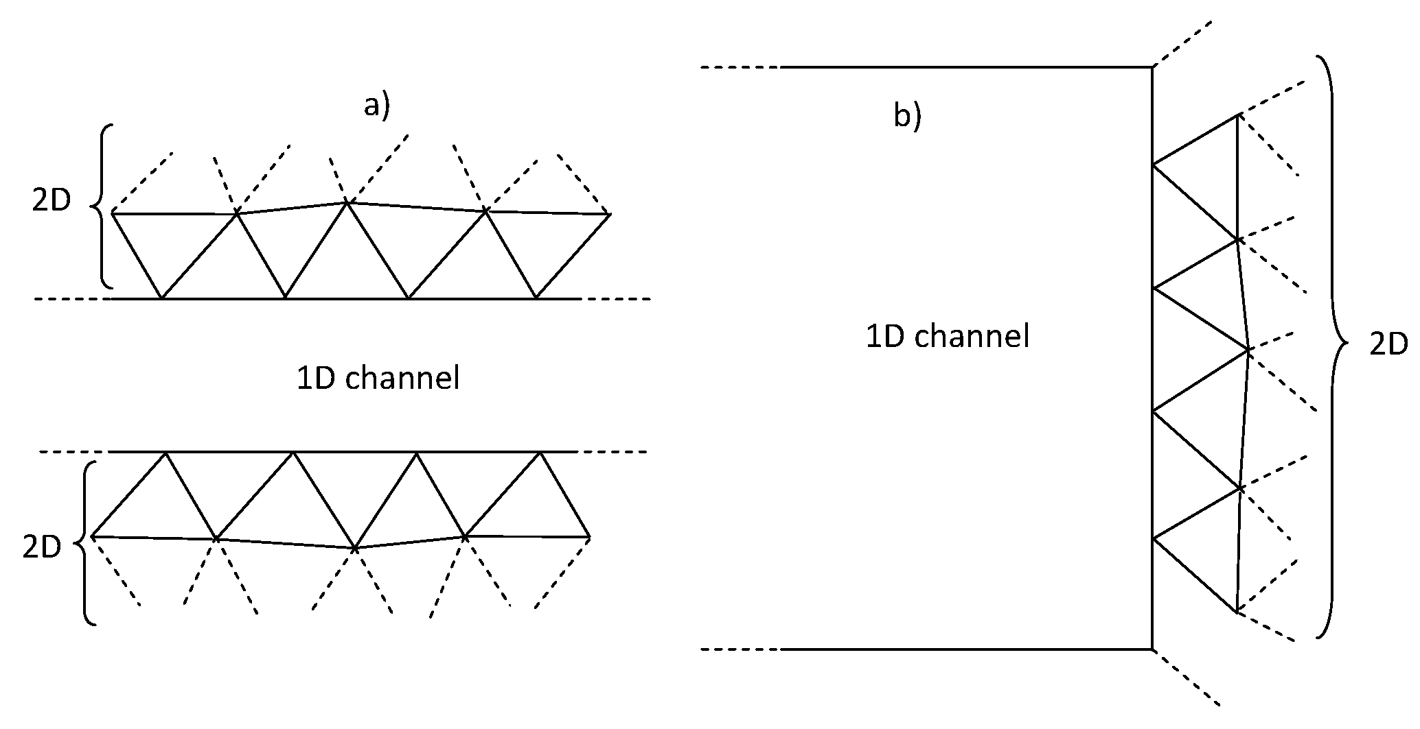
In the following, a new integrated 1D-2D approach, named the FLO model, is proposed for the flow routing on a fixed bed, where the momentum equations are written according to the diffusive approximation. The model domain is split into two parts: the 1D domain, composed of quadrilateral elements aligned according to the known flow direction, and the 2D domain, composed of triangular elements sharing nodes. The boundary nodes of the 2D domain can be located (see Figure 1): (1) on the external boundary of the 1D-2D model; (2) on the vertices of the 1D quadrilateral elements (lateral coupling); (3) on the edges of the quadrilateral elements normal to the flow direction (frontal coupling). The following will show that the use of the diffusive approximation allows the merging of the 1D and 2D boundary computational cells in single cells, as well as the use of implicit methods that guarantee a fast solution, especially when the domain is discretized with strongly irregular meshes. The model is solved in the context of the MArching in Space and Time (MAST) numerical procedure [18], where the solution at the end of each time step is sought through a fractional time step procedure, splitting the original problem into a prediction plus a correction sub-problem.

The paper is organized as follows. At first, the governing equations and the methodology of the fractional step are presented. Subsequently, properties of the required computational mesh and applied fractional time step procedure are described. Finally, the application of the proposed model on academic test cases and real-world situations has been described.

2. 1D Model Equations

The 1D diffusive approximation of the shallow water equations can be written as a system of two first order Partial Differential Equations (PDEs):

$$\frac{\partial \mathsf{\sigma }}{\partial t}+\frac{\partial Q}{\partial s}=p$$

(1)

$$\frac{\partial H}{\partial s}=\frac{\partial h_{\max }}{\partial s}+\frac{\partial z_b}{\partial s}=-J$$

(2)

where t is the time, s is the 1D spatial coordinate measured along the flow direction in the main channel, σ is the transverse 1D cross-section, Q is the 1D flow rate, z_b is the topographic channel bottom level (the topographic elevation of the deepest point in the channel cross-section), H is the water level (or potential or piezometric head), the sum of the maximum water depth h_max in the 1D cross-section and of z_b, H = h_max + z_b, p is the source term (i.e., the inlet flow rate per unit length) and J is the friction slope. Discharge Q is related to J through the relationship:

$$Q=Q_{sp}\sqrt{J}$$

(3)

where Q_sp is a function of h_max, of the bed roughness and of the section geometry, called in the following conveyance and computed as a function of h_max according to [19]. Equation (1) is the mass conservation equation, and Equation (2) is the momentum conservation equation where terms not proportional to acceleration due to gravity have been neglected according to the diffusive hypothesis. Equations (2) and (3) can be merged in Equation (1), to get:

$$\frac{\partial \mathsf{\sigma }\left(H\right)}{\partial t}-\frac{\partial }{\partial s}(Q_{sp}(H)\frac{{\nabla }_{s}H}{\sqrt{\left|{\nabla }_{s}H\right|}})=p$$

(4)

which has to be solved in the H unknown.

3. 2D Model Equations

The 2D diffusive form of the shallow water equations can be written as a system of three first order partial differential equations:

$$\frac{\partial H}{\partial t}+\frac{\partial uh}{\partial x}+\frac{\partial vh}{\partial y}=p$$

(5)

$${\nabla }_{x}H+J\frac{u}{\sqrt{u^2+v^2}}=0$$

(6a)

$${\nabla }_{y}H+J\frac{v}{\sqrt{u^2+v^2}}=0$$

(6b)

where h and z are respectively the water depth and the topographic elevation in the 2D domain, H = h + z is the previously-defined water level, u and v are the x and y vertically-averaged velocity components, ${\nabla }_{x\left(y\right)}H$ is the component of the spatial gradient of the piezometric head in the x(y) direction and J is the energy slope in the velocity direction. Equation (5) is the mass conservation equation, and Equation (6a) and (6b) are the momentum equations in the x and y directions.

Almost all of the research and commercial SW codes compute the energy slope J according to the following formula:

$$J=\frac{n^2\left(u^2+v^2\right)}{h^{4/3}}$$

(7)

which is obtained from the Manning formula applied to a rectangular section normal to the flow direction, with a laterally horizontal bed, unit width and frictionless walls. Equation (7) is consistent with the 2D SW hypothesis of small slope in all directions of the computational domain, including the direction normal to the main flow velocity. On the other hand, the application of the 2D model to the domain including rivers where the lateral slope of the bed can be much larger than zero provides a discrepancy between the 1D and the 2D model in areas of the 2D domain close to the 1D domain.

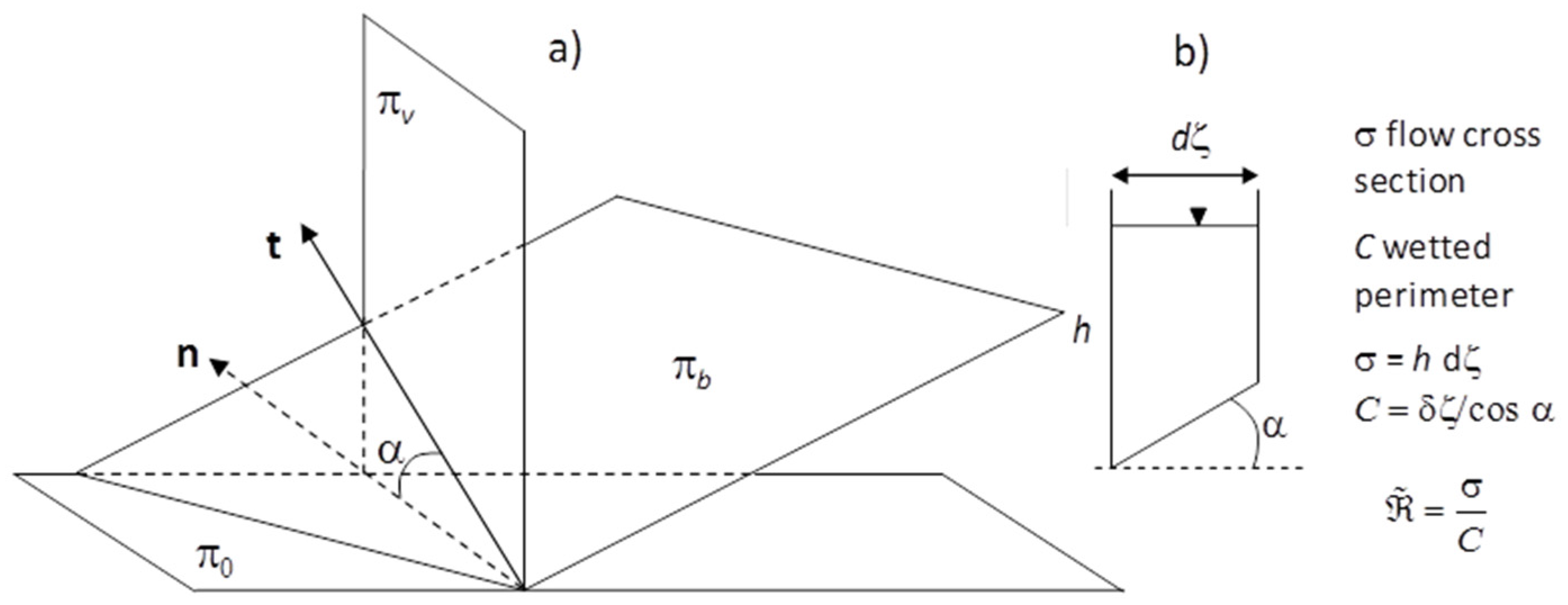
This difference can be observed by computing by the Manning formula the energy slope in a channel with a trapezoidal section, unit width and frictionless vertical walls, where the bed slope in the lateral direction normal to flow can be different from zero.

Call π₀ the horizontal plane, π_b the bottom plane and π_v the vertical plane orthogonal to flow velocity vector (see Figure 2a). Call n and t the unit vectors normal to flow velocity and parallel respectively to π₀ (n) and to π_b (t) (see Figure 2a). Let α be the angle, in the vertical plane, between t and n (see Figure 2a). The energy slope is, according to the Manning formula:

$$J=\frac{n^2\left(u^2+v^2\right)}{{\tilde{\Re }}^{4/3}}$$

(8)

where (see Figure 2b):

$$\tilde{\Re }=h\cos \mathsf{\alpha }$$

(9)

This implies that Equation (7) can be changed into:

$$J=\frac{n^2\left(u^2+v^2\right)}{h^{4/3}{\left(\cos \mathsf{\alpha }\right)}^{4/3}}$$

(10)

which is equivalent to Equation (7) only if the α angle is very small. In the 2D model, cosα can be computed as:

$$\cos \mathsf{\alpha }=\frac{l_n{l}_t+m_n{m}_t+r_n{r}_t}{\sqrt{\left(l_n^2+m_n^2+r_n^2\right)}\sqrt{\left(l_t^2+m_t^2+r_t^2\right)}}$$

(11a)

where l_n(t), m_n(t) and r_n(t) are the directional parameters of n(t), respectively equal to:

$$\begin{array}{c}{l}_n={\nabla }_{y}H{m}_n=-{\nabla }_{x}H{\mathrm{r}}_n=0\\ l_t={\nabla }_{y}H\cdot p{a}_c{m}_t=-{\nabla }_{x}H\cdot p{a}_c{\mathrm{r}}_t={\nabla }_{x}H\cdot p{a}_b-{\nabla }_{y}H\cdot p{a}_a\end{array}$$

(11b)

and pa_a, pa_b and pa_c are the director cosines of the vector orthogonal to the bottom plane. If a triangular mesh with peace-wise linear variation of H and z inside each element is used, the parameters at the l.h.s. of Equation (11b) will be constant inside each element.

Merging Equations (10) and (11) into Equation (6) and Equation (6) into Equation (5), we get for the 2D model the following equation that has to be solved in the H unknown:

$$\frac{\partial H}{\partial t}-\frac{\partial }{\partial x}(\frac{h^{5/3}\text{cos}{\mathsf{\alpha }}^{2/3}}{n\sqrt{|\nabla H|}}-\frac{\partial H}{\partial x})-\frac{\partial }{\partial y}(\frac{h^{5/3}\text{cos}{\mathsf{\alpha }}^{2/3}}{n\sqrt{|\nabla H|}}-\frac{\partial H}{\partial y})=p$$

(12)

4. Initial and Boundary Conditions

Initial and boundary conditions have to be specified to make Problems (4) and (12) well posed. Boundary conditions may be of a Dirichlet (prescribed piezometric head or water depth) or a Neumann (prescribed flux) type. If Ω is the spatial domain where Problems (4) and (12) are defined, initial and boundary condition can be written as:

$$\begin{array}{c}h\left(x,t\right)=h_D\left(x,t\right)\text{\hspace{1em}or\hspace{1em}}H\left(x,t\right)=H_D\left(x,t\right),x\in {\Gamma }_D\\ q\left(x,t\right)\cdot n=g_N\left(x,t\right),x\in {\Gamma }_N\\ h\left(x,0\right)=h_0\text{\hspace{1em}or\hspace{1em}}H\left(x,0\right)=H_0,x\in \mathsf{\Omega }\end{array}$$

(13)

where Γ = Γ_D U Γ_N is the boundary of Ω, Γ_D and Γ_N are the portions of Γ where Dirichlet and Neumann boundary conditions hold, respectively, H_D and h_D are the assigned Dirichlet values for H and h, g_N is the assigned Neumann flux, q(x, t) is the boundary flow rate vector, n is the unit outward normal to the boundary, x = (x, y) and the subscript 0 marks the initial state in the domain.

5. The Fractional Time Step Procedure

The numerical solution of Equations (4) and (12) in the H unknown is attained by means of a time-splitting approach, briefly described in the following. We refer the reader to the cited papers for more details.

Assume a general system of balance laws:

$$\frac{\partial U}{\partial t}+\nabla \cdot F\left(U\right)=B\left(U\right)$$

(14)

where U is the unknown variable, F(U) is the flux vector and B(U) is a source term. Applying a fractional time step procedure, we compute the solution of Equation (14) at the end of each time step by the solution of the following systems [14]:

$$predictionsystem{U}^{k+1/2}-U^k+\nabla \cdot {\displaystyle \underset{0}{\overset{\mathsf{\Delta }t}{\mathsf{\int }}}{F}^{p}dt}={\displaystyle \underset{0}{\overset{\mathsf{\Delta }t}{\mathsf{\int }}}{B}^{p}dt}$$

(15a)

$$correctionsystem{U}^{k+1}-U^{k+1/2}+\nabla \cdot {\displaystyle \underset{0}{\overset{\mathsf{\Delta }t}{\mathsf{\int }}}Fdt}-\nabla \cdot {\overline{F}}^p\mathsf{\Delta }t={\displaystyle \underset{0}{\overset{\mathsf{\Delta }t}{\mathsf{\int }}}Bdt}-{\overline{B}}^p\mathsf{\Delta }t$$

(15b)

where ${\overline{F}}^p$ and ${\overline{B}}^p$ are the mean in time numerical flux and source terms computed along the prediction step and U^k+1/2 and U^k+1 are the unknown variables computed respectively at the end of the prediction and the correction phases. Indices k, k + 1/2, k + 1 respectively mark the beginning of the time step (time level t^k), the end of the prediction step (time level t^k+1/2) and the correction step (time level t^k+1). Integrals ${\overline{F}}^p\mathsf{\Delta }t$ and ${\overline{B}}^p\mathsf{\Delta }t$ will be estimated “a posteriori” after the solution of the prediction problem, according to the procedure explained in [14]. In the present case, we have:

$$1Dmodel\{\begin{array}{l}U=H\\ F=-Q_{sp}\left(H\right)\frac{{\nabla }_{s}H}{\sqrt{\left|{\nabla }_{s}H\right|}}\\ B=p\end{array}2Dmodel\{\begin{array}{l}U=H\\ F=-\frac{h^{5/3}\cos {\mathsf{\alpha }}^{2/3}}{n\sqrt{\left|\nabla H\right|}}\nabla H\\ B=p\end{array}$$

(16)

and we set:

$$1Dmodel\{\begin{array}{l}{F}^p=-Q_{sp}\left(H\right)\frac{{\left({\nabla }_{s}H\right)}^k}{\sqrt{{\left|{\nabla }_{s}H\right|}^k}}\\ B^p=B\end{array}2Dmodel\{\begin{array}{l}{F}^p=-\frac{h^{5/3}\cos {\mathsf{\alpha }}^{2/3}}{n\sqrt{{\left|\nabla H\right|}^k}}{\left(\nabla H\right)}^k\\ B^p=B\end{array}$$

(17)

Observe that the flux formulation differs from the original one (Equations (4) and (12)) in the time level of spatial gradients of H, which are kept constant in time in the prediction step and equal to the values computed at the end of the previous time step. The prediction equation to be solved along the given time step is:

$$1Dmodel\frac{\partial \mathsf{\sigma }\left(H\right)}{\partial t}-\frac{\partial }{\partial s}\left(Q_{sp}\left(H\right)\frac{{\nabla }_s{H}^k}{\sqrt{\left|{\nabla }_s{H}^k\right|}}\right)=p$$

(18)

$$2Dmodel\frac{\partial H}{\partial t}-\frac{\partial }{\partial x}\left(\frac{h^{5/3}\cos {\mathsf{\alpha }}^{2/3}}{n\sqrt{\left|\nabla H^k\right|}}\frac{\partial H^k}{\partial x}\right)-\frac{\partial }{\partial y}\left(\frac{h^{5/3}\cos {\mathsf{\alpha }}^{2/3}}{n\sqrt{\left|\nabla H^k\right|}}\frac{\partial H^k}{\partial y}\right)=p$$

(19)

The prediction problem is solved in its integral form, as shown in the following, while the correction problem is solved in its differential linearized form:

$$1Dmodel\frac{\partial \mathsf{\eta }}{\partial t}L\left(h^{km}\right)-\frac{\partial }{\partial s}\left({\overline{Q}}_{sp}\frac{1}{\sqrt{\left|{\nabla }_s{H}^k\right|}}\frac{\partial \left(\mathsf{\eta }-\mathsf{\vartheta }\right)}{\partial s}\right)=0$$

(20)

$$2Dmodel\frac{\partial \mathsf{\eta }}{\partial t}-\frac{\partial }{\partial x}\left(\frac{{\left(h^{km}\right)}^{5/3}\cos {\mathsf{\alpha }}^{2/3}}{n\sqrt{\left|\nabla H^k\right|}}\frac{\partial \left(\mathsf{\eta }-\mathsf{\vartheta }\right)}{\partial x}\right)-\frac{\partial }{\partial y}\left(\frac{{\left(h^{km}\right)}^{5/3}\cos {\mathsf{\alpha }}^{2/3}}{n\sqrt{\left|\nabla H^k\right|}}\frac{\partial \left(\mathsf{\eta }-\mathsf{\vartheta }\right)}{\partial y}\right)=0$$

(21)

in the unknown η, with:

$$\mathsf{\eta }=H-H^{k+1/2}\text{\hspace{1em}and\hspace{1em}}\mathsf{\vartheta }=H^k-H^{k+1/2}$$

(22)

and h^km is a water depth value in the computational cell obtained by local mass balance, computed as explained in [14], as well as the ${\overline{Q}}_{sp}$ coefficient in Equation (20). The initial condition is η = 0, and L(h^km) in Equation (20) is the water surface width corresponding to h^km.

After some simple manipulations, it can be shown that Equations (18) and (19) are kinematic, with only one characteristic line passing through each (x, t) point [14,18]. The prediction PDE system is equivalent to a single non-linear convection equation, the function of the gradient of the piezometric head at time level t^k, while the correction system has the functional characteristics of a pure diffusive problem.

The convective prediction problem has to be solved by giving the known discharge as the boundary condition to the upstream nodes. The diffusive correction system is solved by setting to zero diffusive flux in the upstream boundary nodes and by giving to the downstream nodes the proper boundary condition required to satisfy the boundary conditions of the original Problems (4)–(12). For example, if the downstream water level is known and equal to H*, the correction η in the downstream boundary will be set equal to: $\mathsf{\eta }=H*-H^{k+1/2}$.

6. Computational Mesh Properties and Computational Cells

The governing PDEs (4) and (12) are discretized over an unstructured hybrid mesh, with triangular and quadrilateral elements. 1D channels are discretized using quadrilateral elements, with one couple of opposite edges overlapping the trace of two river sections and the other couple connecting their ends. The trace of each river section is extended up the minimum topographic elevation where 1D flow conditions are expected. The 2D domain covers the floodplains, and it is discretized by triangular elements satisfying the generalized Delaunay conditions [14].

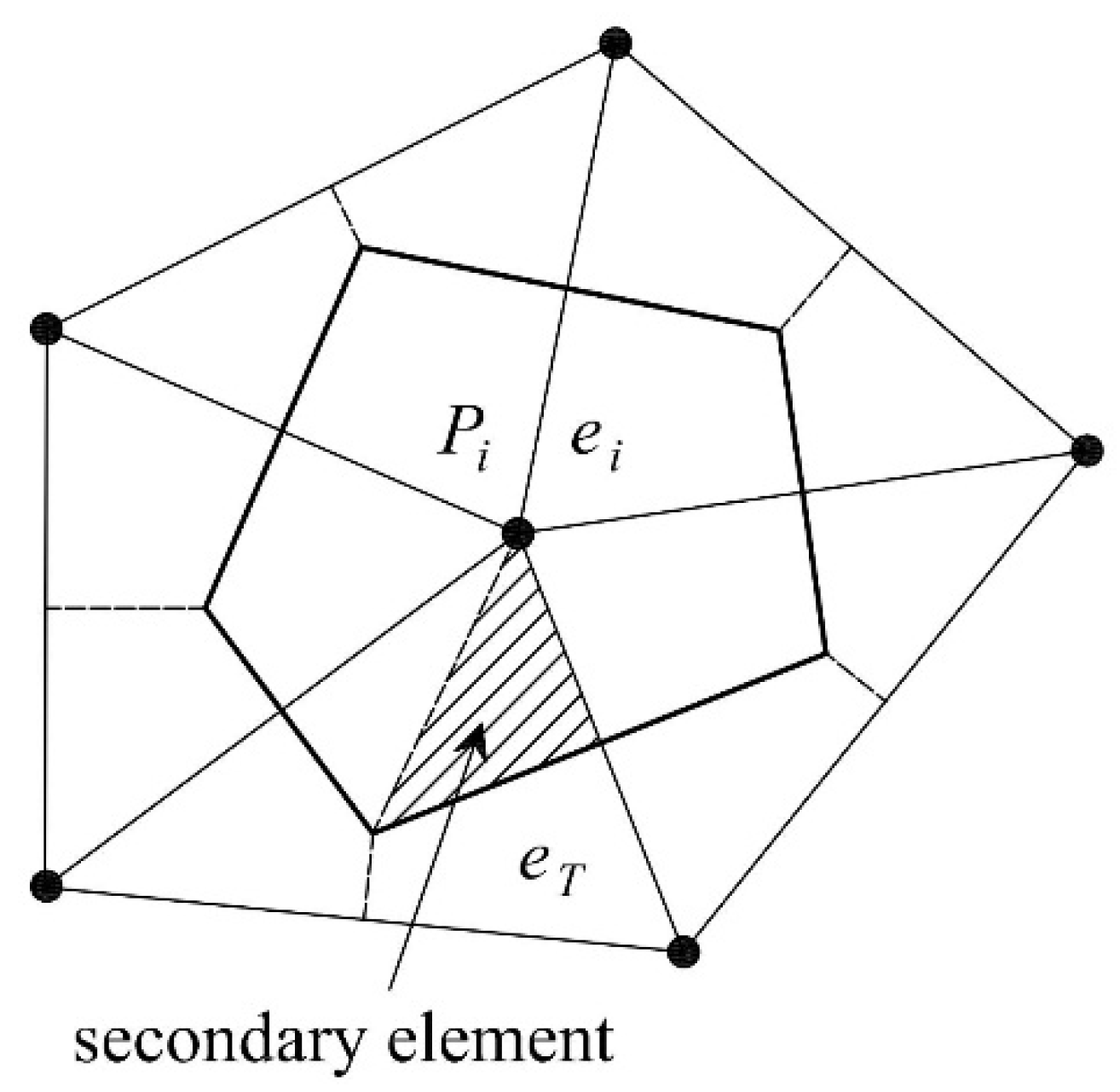
Let ${\mathsf{\Omega }}_{2D}\subset {\Re }^2$be a 2D bounded domain, Ω_h,2D a polygonal approximation of Ω_2D and T_h an unstructured Delaunay-type triangulation of Ω_h,2D [14]. The triangulation T_h is called the basic mesh, and the triangle k_T $\in$ T_h is called the primary element. Let P_h = $\{P_{i}i=1,\dots N\}$ be the set of all vertices (or nodes) of all k_T $\in$ T_h and N the total number of nodes. The dual finite volume e_i associated with vertex P_i is the closed polygon given by the union of sub-triangles resulting from the subdivision of each triangle of T_h connected to node P_i by means of its axes (see Figure 3). In the following part of the paper, the dual volumes e are called also (computational) cells.

The dual finite volume e_i, previously defined, is called the Voronoi cell or the Thiessen polygon [20]. The vertices of the Voronoi cells are the circumcenters of the Delaunay triangulation. Area A_V,i of the Voronoi cell i associated with node P_i is computed as:

$$A_{V,i}=\frac{1}{3}{\displaystyle \sum _{n=1,N_t}\left|k_n\right|}$$

(23)

where $\left|k_n\right|$ is the area of each of the N_t triangles sharing node P_i. Storage capacity is assumed concentrated in the cells (nodes) in the measure of 1/3 of the area of all of the triangles sharing each node. Let H_i be the water level in node P_i and $h_{P_i}$ the corresponding water depth, defined as:

$$h_{P_i}=\text{max}\left(\left(H_i-z_{P_i}\right),0\right)$$

(24)

with $z_{P_i}$ the topographic node elevation. Horizontal area A_i of cell i is computed as:

$$A_i=A_{V,i}{\mathsf{\delta }}_i$$

(25)

where δ_i = 1 if $h_{P_i}>0$, and δ_i = 0 otherwise.

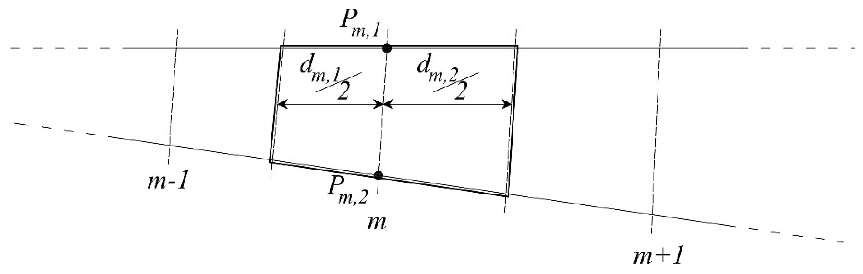
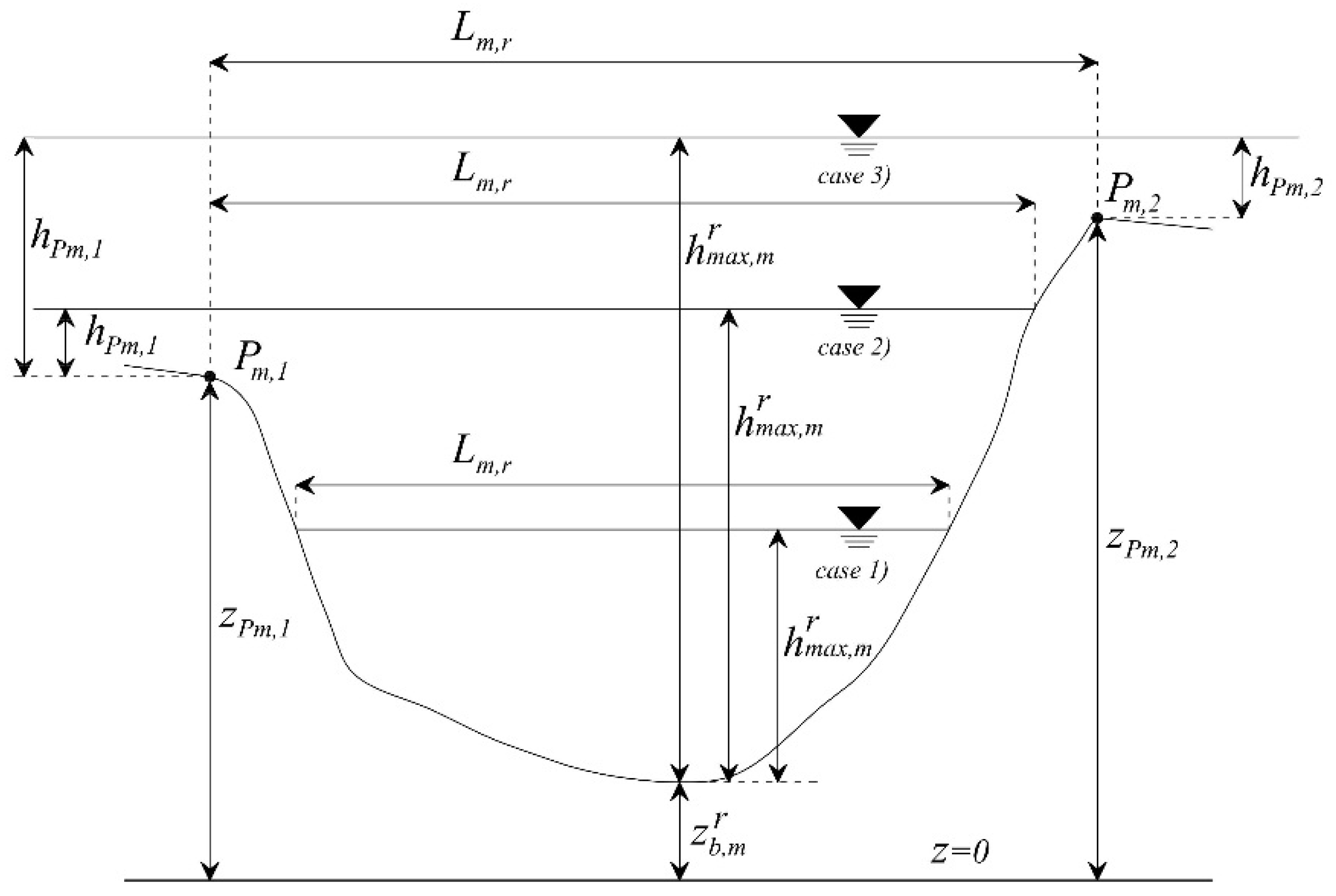
The computational domain includes generally also 1D channels, made of quadrilateral 1D elements. Let m be the index of a 1D section and m + 1 and m − 1 the indices of the two neighboring ones, respectively upstream and downstream m (see Figure 4). Call P_m,1 and P_m,2 the points at the ends of section m and d_m,r the average distance between sections m and m − 1 (r = 1) or between sections m and m + 1 (r = 2). Computational cell i associated with section m in the 1D domain is given by the two halves of downstream and upstream 1D elements next to section m, if existing. We assume P_m,1 and P_m,2 to have the same water level H_i corresponding to the computational cell i associated with section m. Let $h_{max,m}^1$ and $h_{max,m}^2$ be the two maximum water depths upstream and downstream of the discontinuity along the 1D section, computed as:

$$h_{max,m}^r=\text{max}\left(0,\left(H_i-z_{b,m}^r\right)\right)r=1,2$$

(26)

where $z_{b,m}^r$ are the bottom elevations associated with each measured section. According to Equation (26), one or both water depths can be equal to zero if the water level is less than one or both of the bottom elevations. If the bottom discontinuity is zero, $h_{max,m}^1=h_{max,m}^2$.

The σ(h) and L(h) functions upstream and downstream of the bottom discontinuity provide the two cross-sections σ_m,1 and σ_m,2 and the two water surface widths L_m,1 and L_m,2 corresponding to $h_{max,m}^1$ and $h_{max,m}^2$. Horizontal area A_i of computational cell i associated with section m is given by:

$$A_i={\displaystyle \sum _{r=1,2}\left(L_{m,r}\left(h_{max,m}^r\right)\frac{d_{m,r}}{2}\right){\mathsf{\delta }}_{m,r}}$$

(27)

where δ_m,r = 0 if m is a domain boundary section or a 1D section shared with the 2D domain, and δ_m,r = 1 otherwise.

Computational cells around 1D sections coupled with the 2D domain are given by the union of the 1D computational cell and of the Voronoi polygons associated with the node(s) at the section end(s). Call N_m the number of 2D nodes P_m,s shared by 1D section m and the 2D domain and $z_{P_{m,s}}$ their topographic elevation (s = 1, ..., N_m). Let $h_{P_{m,s}}$ be the water depth at node P_m,s, defined as:

$$h_{P_{m,s}}=\text{max}\left(\left(H_i-z_{P_{m,s}}\right),0\right).$$

(28)

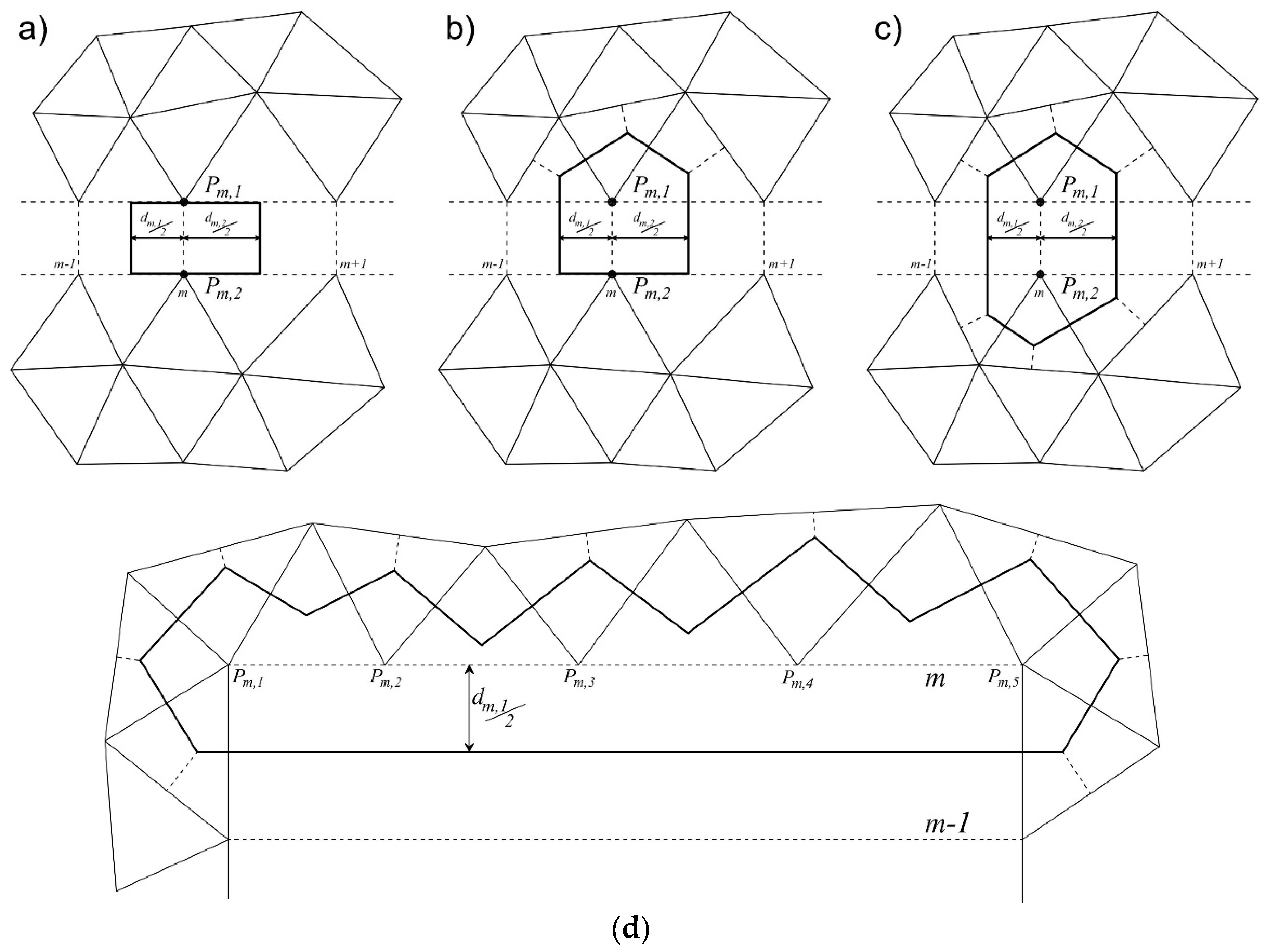
See in Figure 5 the water depths $h_{P_{m,1}}$ and $h_{P_{m,2}}$ in the three situations for lateral coupling. The horizontal area of computational cell i is computed as:

$$A_i={\displaystyle \sum }_{r=1,2}\left(L_{m,r}\left(h_{i,r}\right)\frac{d_{m,r}}{2}\right){\mathsf{\delta }}_{m,r}+{\displaystyle \sum }_{s=1,N_m}{A}_{m,s}{\mathsf{\delta }}_{m,s}$$

(29)

where A_m,s is the Voronoi cell area associated with node P_m,s in the 2D domain (see the previous Equations (23)–(25)), δ_m,s = 1 if node P_m,s is on the trace of section m and $h_{P_{m,s}}>0$, δ_m,s = 0 otherwise, and the other symbols have been specified before.

Figure 6a–c shows the horizontal areas (within the blue lines) of computational cell i for three different geometries, depicted in Figure 5 for the lateral coupling case. Figure 6d shows the horizontal area (within the blue lines) of the computational cell for frontal coupling, assuming $h_{P_{m,s}}>0$ (s = 1,..., 5).

In the following part of the paper, we call “mixed” cells those belonging to both 1D and to 2D domains and N_c the total number of computational cells.

7. Solution of the Prediction Step

The prediction step is solved by applying the MAST methodology [14,18]. MAST’s peculiarity is to solve at each time step one computational cell after the others according to a given order, such that the mean entering flux is known before solving each cell. The requirement for the application of such a procedure is the existence of a potential for the flow field. In the present physical problem, an exact scalar potential of the flow field does exist (the water level), and this allows an easy ordering of the computational cells, from the highest to the lowest water levels. After integration in space, the differential form of the prediction Systems (18) and (19) for cell i is:

$$\frac{d{A}_i\left(H_i\right)}{dt}+{\displaystyle \sum _{j}F{l}_{i,j}^{out}\left(H_i\right)}={\displaystyle \sum _{l}F{l}_{i,l}^{in}}+A_i{p}_i$$

(30)

where summation on the l.h.s. represents the leaving fluxes from cell i to any neighboring downstream (in the potential scale) cell j (with $H_i^k>H_j^k$) and summation on the r.h.s. represents the fluxes entering in cell i from any neighboring upstream cell l (with $H_l^k>H_i^k$). $p_i$ is the source term in cell i (e.g., rain). The relation between A_i and water level H_i has been previously defined in Equations (24)–(29). The outgoing flux $F{l}_{i,j}^{out}$ is a function of H_i since it depends on water depth in cell i, as explained in the following Equations (32) and (33).

The solution of System (31) can be disentangled in the sequential solution of N_c equations by approximating the r. h. s. with its mean value along the given time step, that is by setting:

$$\frac{d{A}_i}{dt}+{\displaystyle \sum _{j}F{l}_{i,j}^{out}}={\displaystyle \sum _l{\overline{Fl}}_{i,l}^{in}}+A_i\overline{p_i}$$

(31)

where ${\overline{Fl}}_{i,l}^{in}$ is the mean in time value of the flux entering from cells l, previously solved, and $\overline{p_i}$ is the $p_i$ mean value. Leaving flux $F{l}_{i,j}^{out}$ between cells i and j is computed as follows.

Case 1: i is a mixed cell. Call m the 1D channel section corresponding to cell i, N_m the number of nodes of sections m (s = 1, ..., N_m), shared with the 2D domain, and call P_m,s any of these nodes.

Case 2: i is a 2D cell. Call P_s the node associated with cell i.

Index n marks any 1D channel section with n ≠ m, having N_n nodes (q = 1, ..., N_n) shared with the 2D domain, and let P_n,q be one of these nodes. Call P_q any node in the 2D domain, not belonging to any 1D section, with P_q ≠ P_s.

We generally assume:

$$F{l}_{i,j}^{out}={\displaystyle \sum _s\left({\displaystyle \sum _{q}f{l}_{s,q}^{2D}{\mathsf{\delta }}_{s,q}^{2D}}\right)}+{\displaystyle \sum _{n}f{l}_{m,n}^{1D}{\mathsf{\delta }}_{m,n}^{1D}}$$

(32)

where the double summation and the second summation on the r.h.s indicate the fluxes leaving from cell i through the sides of respectively the 2D Voronoi polygon and the 1D section cell; index s marks node P_s or P_m,s, depending on whether cell i is a 2D or a mixed cell; q marks node P_q or P_n,q corresponding to cell j. ${\mathsf{\delta }}_{s,q}^{2D}$ is equal to one if nodes P_s (or P_m,s), P_q (or P_n,q) have a common side and $H_i^k>H_j^k$, equal to zero otherwise. ${\mathsf{\delta }}_{m,n}^{1D}$ is equal to one if both i and j are mixed cells, m and n have a common 1D element and $H_i^k>H_j^k$, equal to zero otherwise. Flux is the flux leaving from cell i to any cell j corresponding to node P_q (or P_n,q) sharing a side with node P_s (or P_m,s), $f{l}_{m,n}^{1D}$ is the flux in the 1D channel leaving from cell i to any j cell corresponding to a section n sharing a 1D element with section m.

Flux $f{l}_{s,q}^{2D}$ is computed as:

$$f{l}_{s,q}^{2D}=K_{s,q}^k{h}_s^{5/3}$$

(33)

where h_s is the computed water depth in P_m,s, in Case 1 ($h_s=h_{P_{m,s}}$ as defined in Equation (28)), or in node P_s in Case 2 ($h_s=h_{P_s}$ as defined in Equation (24)). Flux coefficient $K_{s,q}^k$ is computed as explained in [14].

1D flux is computed as follows:

$$f{l}_{m,n}^{1D}=Q_m^r\left(h_{max,m}^r\right)\frac{H_i^k-H_j^k}{\sqrt{\left|H_i^k-H_j^k\right|}}\frac{1}{\sqrt{d_{m,r}}}{\mathsf{\delta }}_{m,n}^{1D}$$

(34)

where $h_{max,m}^r$ is the maximum water depth computed in the 1D section m as in Equation (26), $Q_m^r\left(h_{max,m}^r\right)$ is the conveyance corresponding to $h_{max,m}^r$, d_m,r is a geometric distance (see Figure 7) and r = 1 if n = m − 1, r = 2 if n = m + 1. If m is a measured section; $Q_m^r\left(h_{max,m}^r\right)$ is given by the Q_sp(h) function assigned to the same section. If m is an interpolated section, $Q_m^r\left(h_{max,m}^r\right)$ is obtained by linear interpolation of the two functions Q_sp(h) available in the two upstream and downstream measured sections. If both i and j cells are in the 2D domain, flux $f{l}_{i,j}^{1D}$ is zero.

After the solution of each Ordinary Differential Equations (ODE) (31), the mean in time total flux going from cell i to the neighboring downstream cells can be computed by the local mass balance for cell i, that is:

$${\overline{Fl}}_i^{out}={\overline{Fl}}_i^{in}-\frac{W_i\left(H_i^{k+1/2}\right)-W_i\left(H_i^k\right)}{\mathsf{\Delta }t}+A_i{\overline{p}}_i$$

(35)

where $W_i\left(H_i^{k+1/2\left(k\right)}\right)$ is the water volume stored above cell i at time level k + 1/2 (k) and ${\overline{Fl}}_i^{out}$ and ${\overline{Fl}}_i^{in}$ are respectively the total mean leaving and entering fluxes, with:

$${\overline{Fl}}_i^{in}={\displaystyle {\sum }_l{\overline{Fl}}_{i,l}^{in}}$$

(36)

$H_i^{k+1/2}$ is the final value of the water level computed by the prediction step.

Equation (31) represents the local mass continuity equation integrated in space and time inside the computational cell, and its application guarantees the global conservation of the mass (see Appendix A in [14]), where the proof can be directly applied also to the present case with mixed cells.

The solution of the prediction problem can be classified as “explicit”, because it depends only on the initial state in the cell and on the information (i.e., the flux) coming from the upstream (in the potential scale) cells, previously solved. In standard explicit numerical 1D-2D coupling approaches (see, for example, [10]), the minimum between time step size required in the 1D and 2D domain is computed first, before solving separately of the 1D and 2D domains. The MAST scheme has shown stability with regard to the time step size, also for a Courant number (CFL) much greater than one [21]. For this reason, a unique time step size is used in the proposed approach for the whole domain, without any stability constraint.

In the present formulation, ODE Equation (31) is solved numerically for mixed cells, applying a Runge–Kutta method with a self-adapting time step [22], while an approximated analytical solution is provided for the ODE solution in 2D cells (more details for the analytical solution can be found in [14].

8. Solution of the Correction Step

Diffusive Problems (20) and (21) are solved using the same spatial discretization adopted in the prediction problem, as well as a fully-implicit time discretization. After integration inside each computational cell i, we obtain the following system:

$$\begin{array}{l}\frac{A_i}{\mathsf{\Delta }t}{\mathsf{\eta }}_i+{\displaystyle \sum _j{D}_i^{k,1D}\left({\mathsf{\eta }}_i-{\mathsf{\eta }}_j\right)}+{\displaystyle \sum _j{D}_{i,j}^{k,2D}\left({\mathsf{\eta }}_i-{\mathsf{\eta }}_j\right)}={\displaystyle \sum _j{D}_{i,j}^{k,1D}\left({\mathsf{\vartheta }}_i-{\mathsf{\vartheta }}_j\right)}+{\displaystyle \sum _j{D}_{i,j}^{k,2D}\left({\mathsf{\vartheta }}_i-{\mathsf{\vartheta }}_j\right)}\\ i=1,\mathrm{...},N_c\end{array}$$

(37)

where index j marks any cell connected to i, the second and third terms on the l.h.s. of Equation (38), as well as the first and second terms on the r.h.s., representing the corrective fluxes between cells i and j respectively in the 1D channel and in the 2D domain, computed as a function of the difference of η and θ values (with η and θ defined in Equation (22)).

Assume the same symbols adopted for the prediction step. Call ${\left(f{l}_{s,q}^{2D}\right)}^{k+1/2}$ the leaving flux computed at the end of the prediction step, from cell i to any cell j with $H_j^k\le H_i^k$, through the sides of the 2D Voronoi polygon, as specified in Equations (33) and (34). Call ${\left(f{l}_{m,n}^{1D}\right)}^{k+1/2}$ the leaving flux in the 1D channel computed at the end of the prediction step, from cell i to any j mixed cell with $H_j^k\le H_i^k$, as specified in Equation (34). Define the following coefficients:

$$coe{f}_{s,q}^{2D}=\frac{{\left(f{l}_{s,q}^{2D}\right)}^{k+1/2}{\mathsf{\delta }}_{s,q}^{2D}}{{\left({\displaystyle \sum _{j}F{l}_{i,j}^{out}}\right)}^{k+1/2}}$$

(38a)

and:

$$coe{f}_{m,n}^{1D}=\frac{{\left(f{l}_{m,n}^{1D}\right)}^{k+1/2}{\mathsf{\delta }}_{m,n}^{1D}}{{\left({\displaystyle \sum _{j}F{l}_{i,j}^{out}}\right)}^{k+1/2}}$$

(38b)

where ${\left({\displaystyle \sum _{j}F{l}_{i,j}^{out}}\right)}^{k+1/2}$ is the total leaving flux from cell i computed at the end of the prediction step (see Equation (31)). Let ${\overline{fl}}_{s,q}^{2D}$ be the mean in time leaving flux, through the sides of the 2D Voronoi polygon, from cell i to any j cell corresponding to any 2D node connected with node P_m,s (or P_s) and ${\overline{fl}}_{m,n}^{1D}$ the mean in time leaving flux in the 1D channel from cell i to any linked mixed cell j. These mean fluxes are computed respectively as:

$${\overline{fl}}_{s,q}^{2D}={\overline{Fl}}_i^{out}coe{f}_{s,q}^{2D}$$

(39a)

and:

$${\overline{fl}}_{m,n}^{1D}={\overline{Fl}}_i^{out}coe{f}_{m,n}^{1D}$$

(39b)

with the total mean in time leaving flux ${\overline{Fl}}_i^{out}$ defined in Equation (49).

Flux coefficient $D_{i,j}^{k,2D}$ in Equation (54) is computed as:

$$D_{i,j}^{k,2D}={\displaystyle \sum _{g=1,2}\frac{c_{s,q}^g{E}_g^k}{d_{sq}}{\left(h_l^{km}\right)}^{5/3}{\mathsf{\delta }}_g}$$

(40)

and $h_l^{km}$ is computed as follows. If $H_i^k\ge H_j^k$, $h_l^{km}$ is the water depth in node P_m,s (or P_s) given by:

$$h_l^{km}={\left(\frac{{\displaystyle \sum _q{\overline{fl}}_{s,q}^{2D}{\mathsf{\delta }}_{s,q}^{2D}}}{{\displaystyle \sum _q{K}_{s,q}^k{\mathsf{\delta }}_{s,q}^{2D}}}\right)}^{3/5}$$

(41)

where flux coefficients $K_{s,q}^k$ are computed as explained in [14]. If $H_i^k\le H_j^k$, indices s and q in Equation (42) have to be commuted.

Coefficients $c_{s,q}^g$, $E_g^k$ and d_sq in Equation (40) have been already defined for the prediction step; g is the number of triangles (one or two) sharing side $\overrightarrow{P_{m,s}{P}_{n,q}}$ (or $\overrightarrow{P_{m,s}{P}_q}$); δ_g = 1 if the g-th triangle does exist, and δ_g = 0 otherwise.

If $H_i^k\ge H_j^k$, flux coefficient $D_{i,j}^{k,1D}$ is computed as:

$$D_{i,j}^{k,1D}=\overline{Q_m^r}\frac{{\mathsf{\delta }}_{m,n}^{1D}}{\sqrt{d_{m,n}\left|H_i^k-H_j^k\right|}}$$

(42)

where $\overline{Q_m^r}$is the mean conveyance computed as follows and the other symbols have been specified before.

$$\overline{Q_m^r}={\overline{fl}}_{m,n}^{1D}\frac{\sqrt{\left|H_i^k-H_j^k\right|}}{H_i^k-H_j^k}\sqrt{d_{m,n}}{\mathsf{\delta }}_{m,n}^{1D}$$

(43)

with ${\overline{fl}}_{m,n}^{1D}$ defined in Equation (39b). If $H_i^k\le H_j^k$, indices m and n have to be commuted in both Equations (42) and (43).

Fully implicit time discretization provides unconditional stability, along with some approximation error in the solution [23]. The approximation error is small because its magnitude is of the same order of the computed correction η, and the source term on the r. h. s. of Equation (37) goes to zero along with the time step size. This implies that the absolute error in the estimation of the piezometric correction will only weakly affect the piezometric final value computed at time level k + 1.

The linear system resulting from Equation (37) is well conditioned, with a matrix that is always symmetric, positive definite and strictly diagonally dominant, even in the case of Delaunay triangulations with obtuse triangles [14]. A preconditioned conjugate gradient method is used for its solution.

After the solution of the linear system (37) is obtained in the η unknowns, the piezometric heads H at the end of the time step are obtained as:

H^k+1 = H^k+1/2 + η

(44)

Similarly to the prediction step, the proof provided in Appendix A in [14], concerning the local and global mass balance of the diffusive step, can be directly applied to the case of mixed cells.

9. Stability of the Solution at Discontinuous Nodes

When the water level in the 1D domain of the mixed-type computational cell j drops below the ground elevation of a 2D node in the same cell (Case 1 of Figure 5), the water level in the same 2D node is equal to the ground level, and a discontinuity appears at the boundary between the 1D and the 2D domains. Call these 2D nodes discontinuous nodes. In this case, the prediction step of the MAST approach can be solved anyway, because discontinuity is not inside triangles, and the piezometric gradients remain uniquely defined. On the opposite side, diffusive fluxes in Equation (37) cannot be computed because, due to the discontinuity, second order derivatives are locally missing. The stability of the sought after solution at each computational cell is guaranteed, in the MAST approach, by the correction and by the resulting diffusive fluxes that are summed to the convective ones. This implies that, in this case, a stable solution can be found neglecting diffusive fluxes only by using very small time steps. To avoid this inconvenience, it is possible to solve the equations of the 2D cells connected with cell j by treating the 2D node inside the mixed cell j as a Dirichlet 2D boundary node with zero water depth and by neglecting the resulting diffusive flux inside the cell. This allows one to rearrange Equation (37) of the i-th 2D cell connected with at least one discontinuous node inside mixed type cells in the following form:

$$\left(\frac{A_i}{\mathsf{\Delta }t}+{\displaystyle \sum _{r\in D_j}{D}_{i,r}^{k,2D}}\right){\mathsf{\eta }}_i+{\displaystyle \sum _{r\notin D_j}{D}_{i,r}^{k,2D}\left({\mathsf{\eta }}_i-{\mathsf{\eta }}_r\right)}={\displaystyle \sum _{r\notin D_j}{D}_{i,r}^{k,2D}\left({\mathsf{\vartheta }}_i-{\mathsf{\vartheta }}_r\right)}+{\displaystyle \sum _{r\in D_j}{D}_{i,r}^{k,2D}{\mathsf{\vartheta }}_r}$$

(45)

where D_j is the set of the mixed type cells with a discontinuous node connected to cell i and r is the index of any cell connected to cell i. The equations of the mixed type cells j become:

$$\frac{A_j}{\mathsf{\Delta }t}{\mathsf{\eta }}_j+{\displaystyle \sum _r{D}_j^{k,1D}\left({\mathsf{\eta }}_j-{\mathsf{\eta }}_r\right)}+{\displaystyle \sum _{r\notin D_i}{D}_{j,r}^{k,2D}\left({\mathsf{\eta }}_j-{\mathsf{\eta }}_r\right)}={\displaystyle \sum _r{D}_{j,r}^{k,1D}\left({\mathsf{\vartheta }}_j-{\mathsf{\vartheta }}_r\right)}+{\displaystyle \sum _{r\notin D_i}{D}_{j,r}^{k,2D}\left({\mathsf{\vartheta }}_j-{\mathsf{\vartheta }}_r\right)}$$

(46)

where D_i is the set of the 2D cells connected to cell j with a discontinuous node.

One of the major merits of the MAST approach is to guarantee local and global mass conservation. This property is lost in transient conditions at discontinuous nodes, because the diffusive fluxes going from the 2D domain to the 1D domain are computed in the mass balance of the corresponding 2D cells, but they are missing in the mass balance of the mixed cells of the 1D domain. The resulting global mass balance error is almost negligible, as shown in one of the following tests.

A flux limiter in the connection between mixed type cell j and 2D cell i has also to be forced in the solution of the prediction step, when the level in cell j raises, along the time step, above the ground elevation of the discontinuous node (Cases 2 or 3 in Figure 5). In this case, the average flux along Δt is zero, because hydraulic connection between the 2D and the 1D domain is missing at the beginning of the time step (when Case 1 holds). In the next step, the convective flux will strongly depend on the distance of the connected 2D nodes from the nodes of the mixed cell and will go to infinity along with the inverse of the same distance. To avoid this inconvenience, in the case of lateral coupling, the following limiter is set for the flux going from the mixed cell to the 2D cell:

$$K_{s,q}^k{h}_s^{5/3}\le L_s{h}_s^k\sqrt{g{h}_s^k}$$

(47)

where L_s is the sum of half lengths of the channels sharing section s and the r.h.s. is the discharge corresponding to the critical condition of the lateral overflow. Coefficient $K_{s,q}^k$ has been already defined for Equation (33). Equation (47) can be approximated with:

$$K_{s,q}^k\le L_s\sqrt{g}$$

(48)

with a relative error less than 20% for h_s < 3 m.

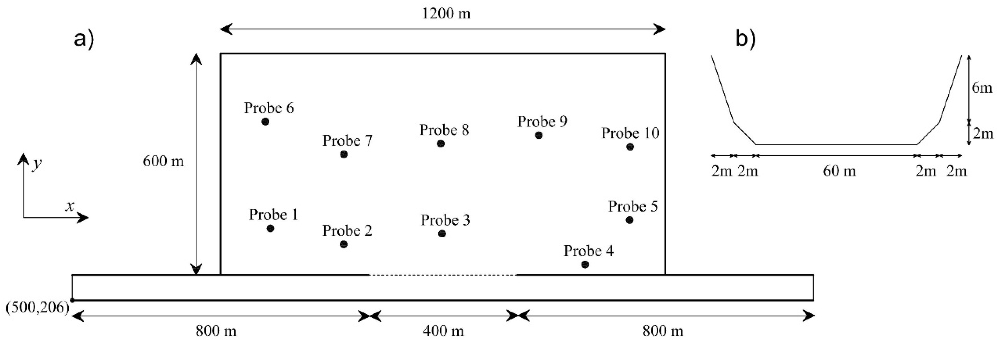
10. Test 1: Comparison with the Results of Morales et al. [10]

In this test, we deal with a hypothetical trapezoidal channel, 2000 m long and a 68-m wide base, connected with a lateral floodplain (see Figure 8a,b). Longitudinal (along the x direction) and transverse (along the y direction) slopes for both the channel and floodplain are respectively 0.001 and zero. The floodplain is closed at the left, top and right boundaries. Manning friction coefficients are 0.03 s/m^1/3 in the floodplain and 0.015 s/m^1/3 in the channel, and sediment transport is not considered. The domain has been discretized with a 1D-2D mesh with lateral coupling, with 6960 triangles, 3600 nodes and 131 1D channel sections (six measured sections). A second unstructured fully 2D mesh has been used, with 29,857 triangles and 15,820 nodes. The triangle number increases in the 2D mesh because of the slope of the trapezoidal cross-section, and a fine mesh is required to represent the topography faithfully. Three scenarios have been selected for the upstream boundary condition: (1) a steady and (2) an unsteady flow in the most upstream channel section; (3) constant net rain, falling homogeneously above all of the floodplain.

In the first case, a constant discharge of 600 m³/s is given as the upstream boundary condition at the channel inlet, and the model is run until convergence to the steady state. The time step is 40 seconds. The proposed coupling procedure computes water depths very similar to the ones obtained over the fully-2D mesh. Due to the different resistance law in the 1D channel and in the floodplain, water depths computed over the coupled 1D-2D mesh are slightly higher than the ones over the 2D mesh, with the highest difference less than 0.01 m. On the opposite side, the results provided by Morales et al. by their coupled procedure show large differences with respect to the ones computed by their 2D model. Morales et al. [10] justify these differences with the choice of the Manning coefficient in the 1D channel and its adjustment due to coupling strategies. See the results of the two models, for both mixed and 2D meshes, shown in

Table 1. Test 1. Steady flow. Steady water depths computed by FLO and Morales et al. [10].

Water Depth (m)
	FLO model		Morales et al., 2013
	coupled 1D-2D	fully 2D	coupled 1D-2D	fully 2D
Probe 1	0.075	0.062	0.000	0.035
Probe 2	0.277	0.278	0.171	0.279
Probe 3	0.501	0.495	0.394	0.513
Probe 4	0.871	0.861	0.870	0.991
Probe 5	0.993	0.983	0.878	0.992
Probe 6	0.020	0.012	0.000	0.000
Probe 7	0.239	0.229	0.000	0.021
Probe 8	0.493	0.475	0.136	0.270
Probe 9	0.747	0.731	0.381	0.510
Probe 10	0.998	0.979	0.660	0.791

.

In the second scenario, a symmetrical triangular hydrograph, with a duration of 16 hours and a peak of 600 m³/s, is assigned in the upstream boundary section. Zero water depth is the Dirichlet downstream boundary condition. The Manning coefficients in the channel and in the floodplain are 0.01605 s/m^1/3 and 0.03 s/m^1/3. For this scenario, four simulations were carried out with a time step size equal to 20, 40, 100 and 400 seconds, in order to evaluate the stability of the model. The CFL number (CFL = VΔt/Δx, where V is the vertical averaged velocity and Δx is the cell length) in the 2D triangle l is computed for the FLO model as:

$$CF{L}_l=\frac{\mathsf{\Delta }t}{\sqrt{\left|k_l\right|}}\frac{{\left({\overline{h}}_l\cos \mathsf{\alpha }\right)}^{2/3}}{n_l}{\left({\left({\nabla }_{x}H\right)}_l^2+{\left({\nabla }_{y}H\right)}_l^2\right)}^{1/4}$$

(49)

where ${\overline{h}}_l$ is the mean water depth value in triangle l, computed as the arithmetic mean of the water depth at the three triangle nodes, and $\left|k_l\right|$ is the triangle area. CFL in 1D section m, associated with the computational cell i, is computed as the maximum value in the two halves of channels, as:

$$CF{L}_m=\text{max}\left(CF{L}_{m,1},CF{L}_{m,2}\right)\text{\hspace{1em}with\hspace{1em}}CF{L}_{m,r}=\frac{\mathsf{\Delta }t}{d_{m,r}/2}\frac{Q_{sp}\left(h_{max,m}^r\right)}{{\mathsf{\sigma }}_{m,r}}\sqrt{\frac{\left|H_i-H_j\right|}{d_{m,r}}}{\mathsf{\delta }}_{m,r}r=1,2$$

(50)

where j is the index of the computational cell corresponding to 1D section upstream or downstream section m, and the other symbols have been specified above.

Maximum CFL values, listed in

Table 2. Test 1. Unsteady flow. Maximum CFL values computed by FLO model.

CFL
	1D domain	2D domain
ΔT = 20 s	147.22	39.73
ΔT = 40 s	295.08	79.41
ΔT = 100 s	742.54	197.96
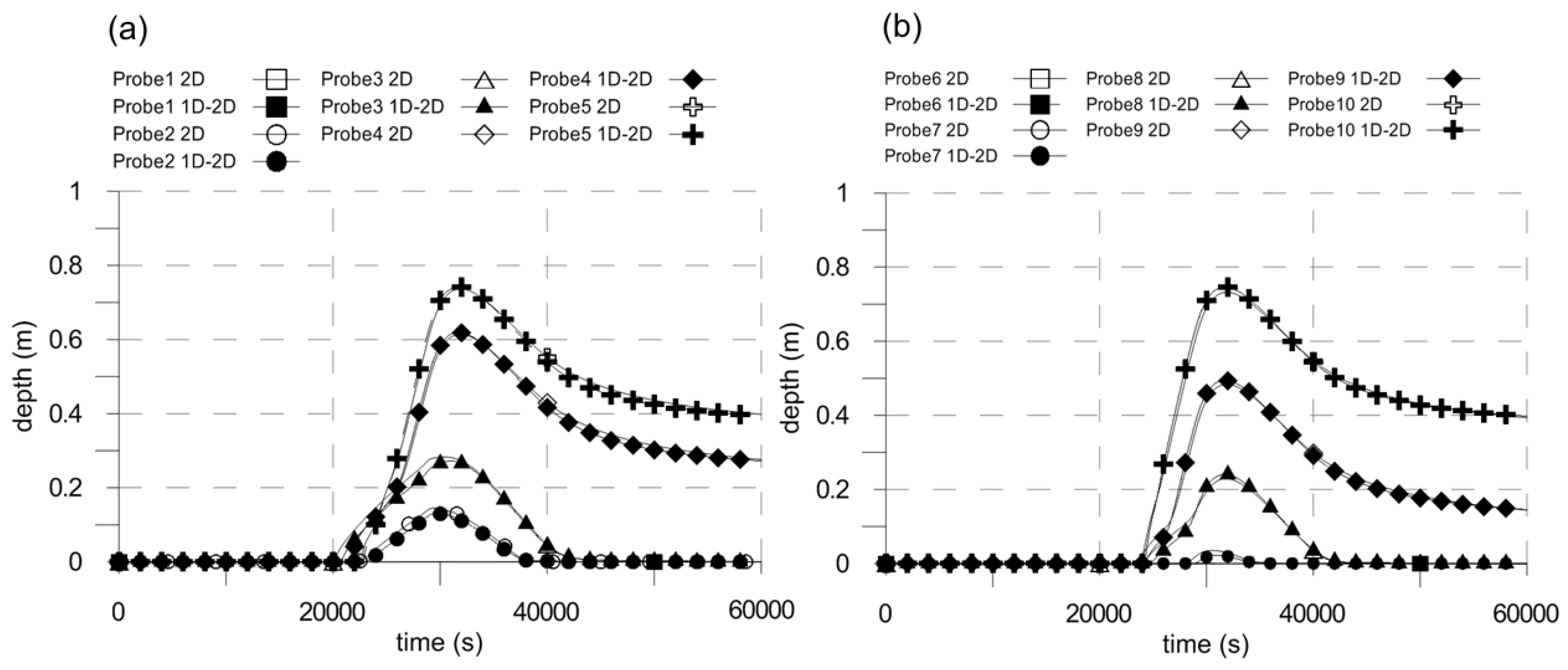
ΔT = 400 s	869.96	2992.40

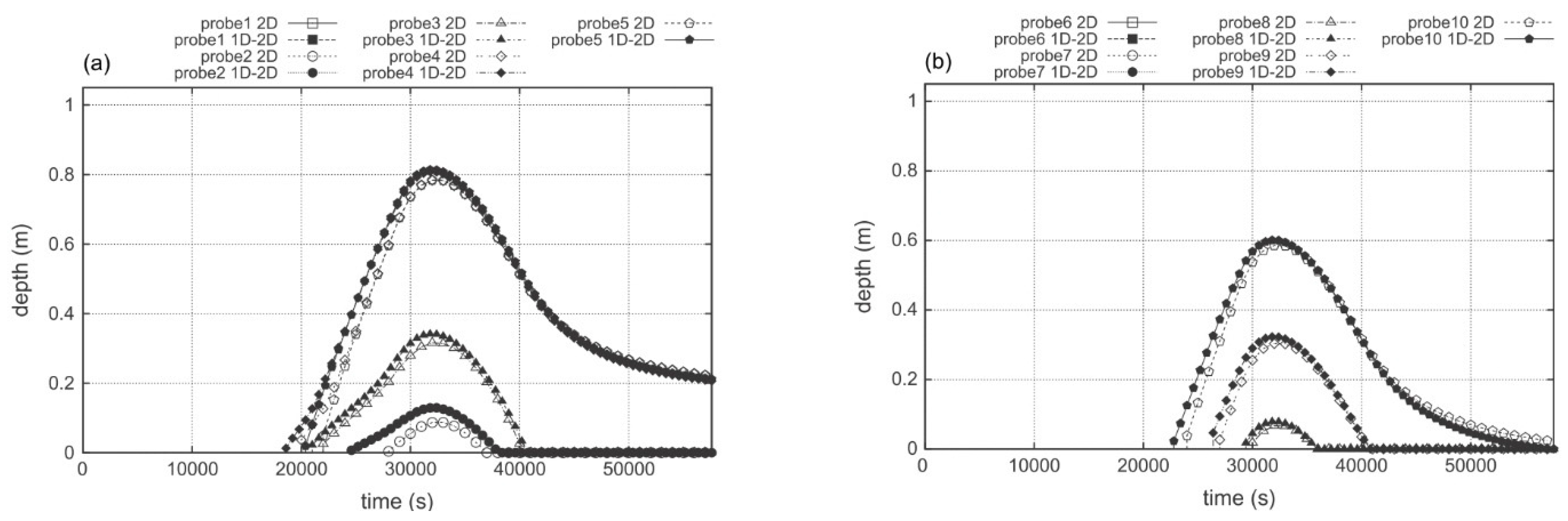
, are all much greater than one. Observe in Figure 9a,b that water depths at Gauges 5 and 10 provided by the FLO model show similar values. This is reasonable, since both gauges are very close to the right floodplain wall (see Figure 8), and the transverse slope of the floodplain is zero. On the other hand, water depths measured at Gauge 4 are different from the ones at Point 5 (in Figure 9a), where Point 4 is closest to the inlet of the floodplain and further away from the wall than Point 5. Observe the opposite in the results provided by Morales et al. 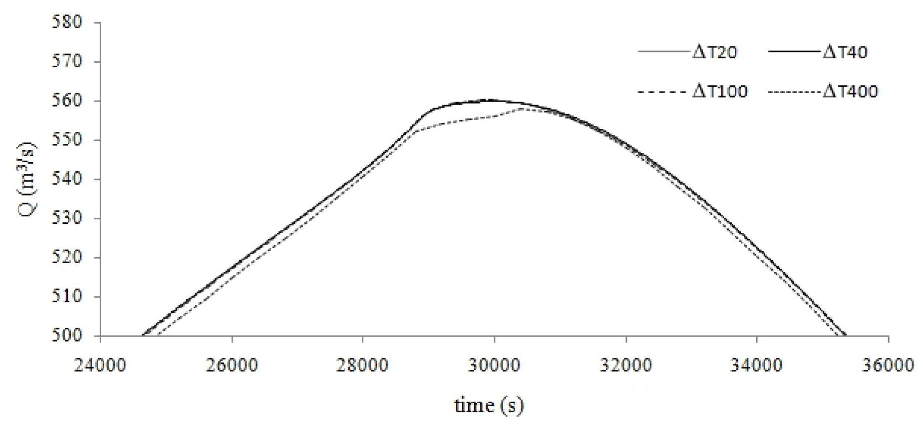[10] and shown in Figure 10, where water depths at Points 4 and 5 are often undistinguishable at the adopted graphic scale, while smaller water depths are computed at Gauge 10 (see Figure 10a,b). For each simulation, the discharges leaving the domain and computed by the FLO model are very similar, and only the peak region is shown in Figure 11. Morales et al. [10] reduced the scatters between their 1D-2D and 2D models’ results by modifying the Manning friction coefficient in the floodplain (see Figures 19 and 20 of their paper). On the opposite, we do not modify the roughness coefficient values with respect to their original values. Moreover, we do not have to solve additional equations at the boundaries between the 1D and the 2D domain, unlike Morales et al. [10].

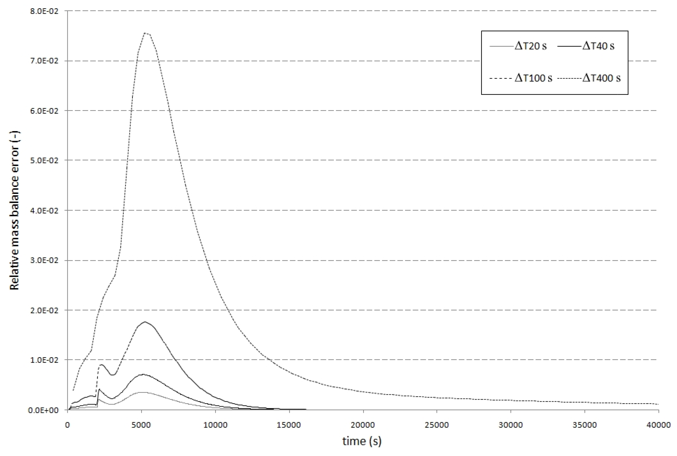
In Scenario 3, initial conditions are the same used for Scenario 1, and the Neumann boundary condition has been replaced with a constant net rainfall, equal to 200 mm/h, applied above all of the floodplain, which provides a stationary entering discharge equal to 42.3 m³/s. The test was carried out with the same time step size used for Scenario 2. The relative mass balance error in the correction step due to the existence of discontinuous nodes is reported for each time step in Figure 12. It has been computed as the ratio between the total discharge neglected in the correction step and the total entering rain volume per unit time. The error obtained with a time step of 40 s (7.10 × 10⁻³) is negligible for practical applications. For higher time steps, FLO returns a higher error, although the outlet discharge hydrograph remains always stable (see Figure 11 and Figure 12). Observe that the hypothesis of instantaneous shift from zero to a finite net rain intensity is quite severe in real applications, and a time step of 40 s corresponds to a maximum CFL = 295 (Table 1).

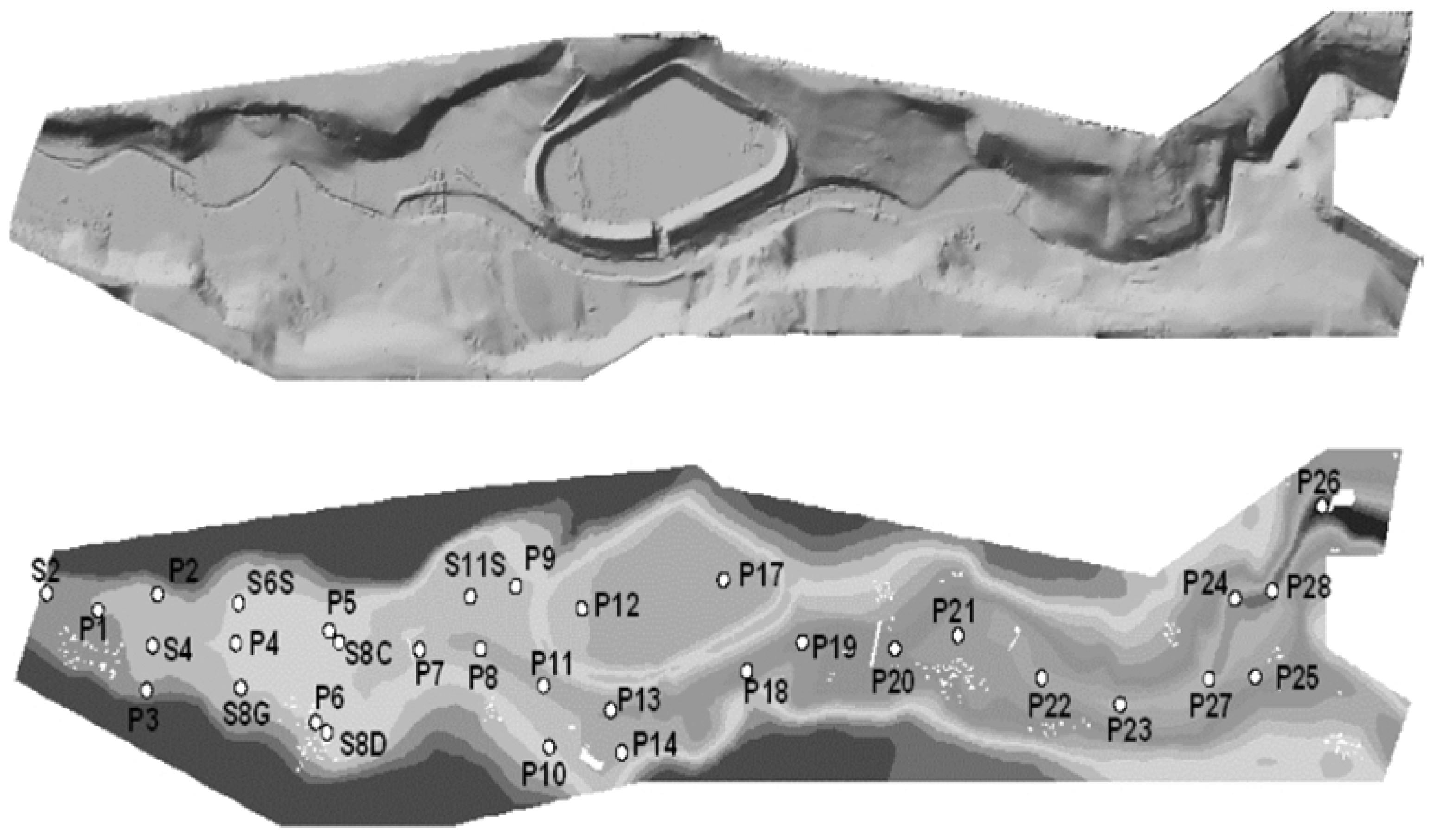
11. Test 2: The Toce River (Italy) Test Case

A physical model at a scale of 1:100 of a reach of the Toce River valley (western Alps, Italy) was reproduced at the ENEL-HYDRO Laboratory in Milan [24]. The model reproduces a reach of the riverbed, the floodplain and a lateral reservoir designed for flood control purposes (see Figure 13a). The physical model approximately covered an area of 50 m × 12 m.

On the upstream side of the model, a tank was installed to provide the input discharge hydrograph, with an initial sharp peak. The water is released from the tank in the model domain, by means of a pump, which can attain the maximum flow rate of 0.5 m³/s (50,000 m³/s in the real scale).

The upstream part of the valley around the river bed is large and flat. On the left bank side of the Toce, approximately in the middle of the domain, there is a storage tank. The position of this tank is very critical, since during catastrophic floods, it can overflow easily. Thirty two outlet piezometers with a diameter of 0.025 m, with the inlet on the surface of the model bed, have been placed below the model, connected either to pressure transducers, for automatic level registrations, or to hydrometers, for a comparison of the measurements in the stationary cases (see Figure 13b).

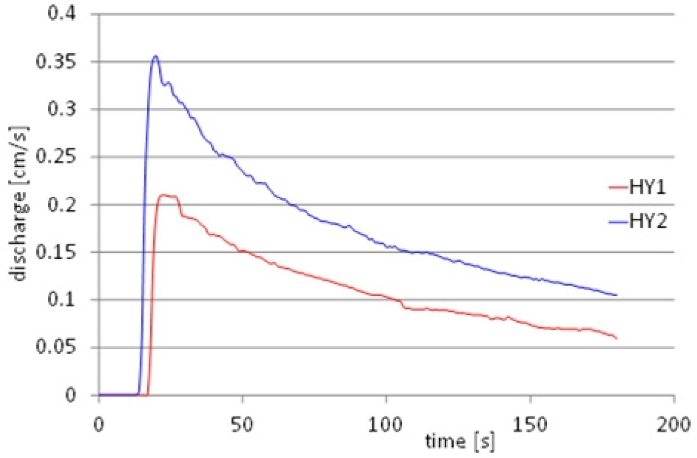
Two different test cases have been carried out in the physical model; one corresponding to the overtopping of the reservoir in the middle of the river, the other without overtopping. The inflow hydrographs at the upstream end of the physical model, without overtopping (HY1) and with overtopping (HY2), are shown in Figure 14. Peak flow for HY1 was 0.2 m³/s (corresponding to 20,000 m³/s at the real scale), while peak flow for HY2 was 0.35 m³/s (35,000 m³/s at the real scale).

Domain discretization has been carried out starting from a 0.05 m × 0.05 m DEM resolution. A frontal coupling approach has been adopted, and a 1D-2D mesh with 35,673 triangles, 18,633 nodes and 272 1D sections (47 measured sections) has been used. The central part of the domain, including the lateral reservoir, is discretized with 2D triangles, while the upstream and downstream parts are discretized as 1D channels. Computed results of the coupled approach have been compared to the corresponding ones obtained over a fully-2D Delaunay mesh with 82,390 triangles and 41,947 nodes.

The Manning friction coefficient n is set equal to 0.0162 s/m^1/3. This value has been taken from the literature (e.g., [24,25] and the cited references) and has not been previously calibrated.

The bed was assumed initially dry. The applied boundary conditions are the discharge hydrographs measured in the outlet pipe of the lab tank (upstream condition) and the zero water level second order derivative (downstream condition). Time step sizes is 0.1 s, and the maximum values of CFL numbers computed over the coupled mesh are 97 and 7.5, respectively, in the 2D domain and in 1D channels, for HY1, and 130 and 11.1, respectively, in 2D domain and 1D channels for and HY2. Similar values to the ones computed in the 2D portions of domain have been obtained over the fully-2D mesh.

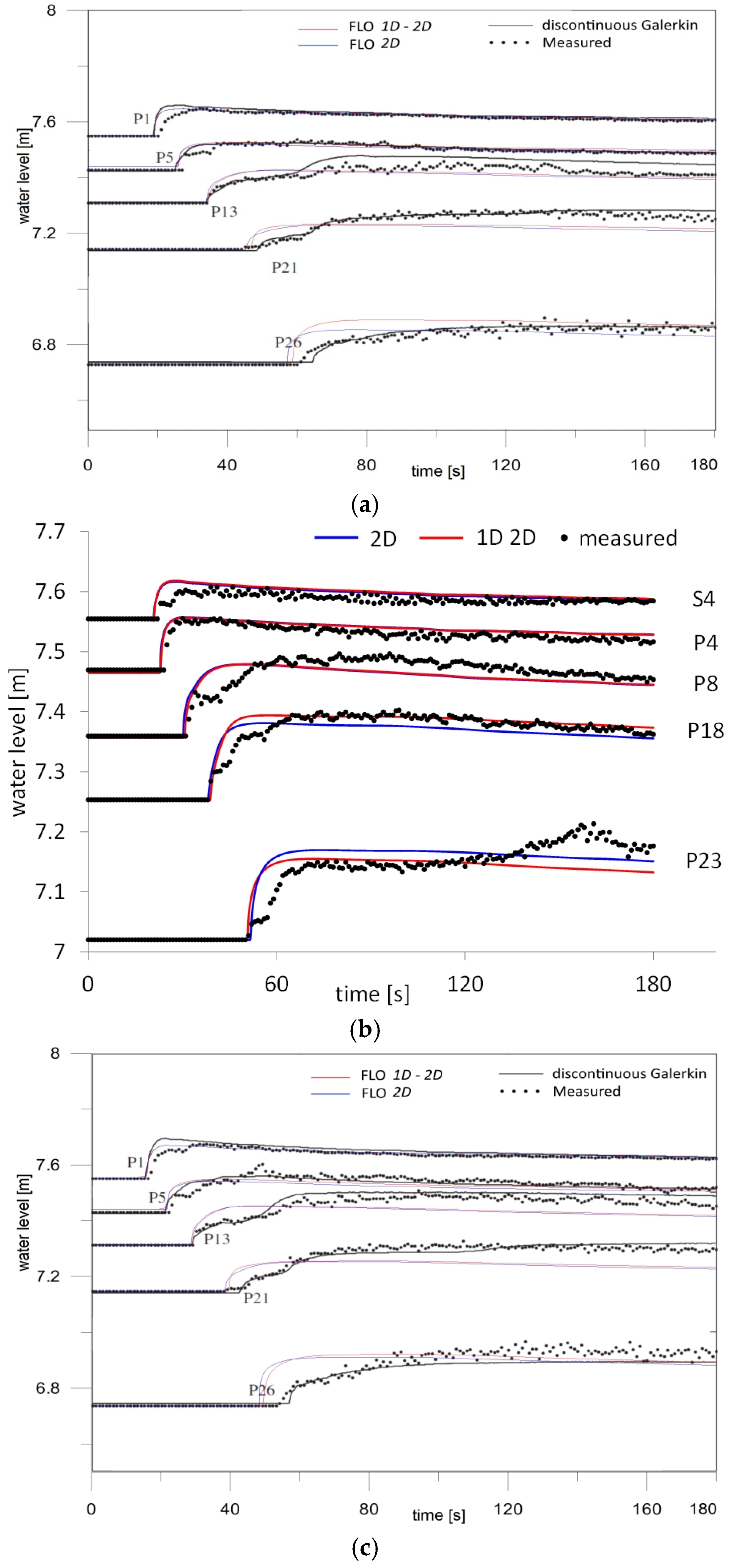
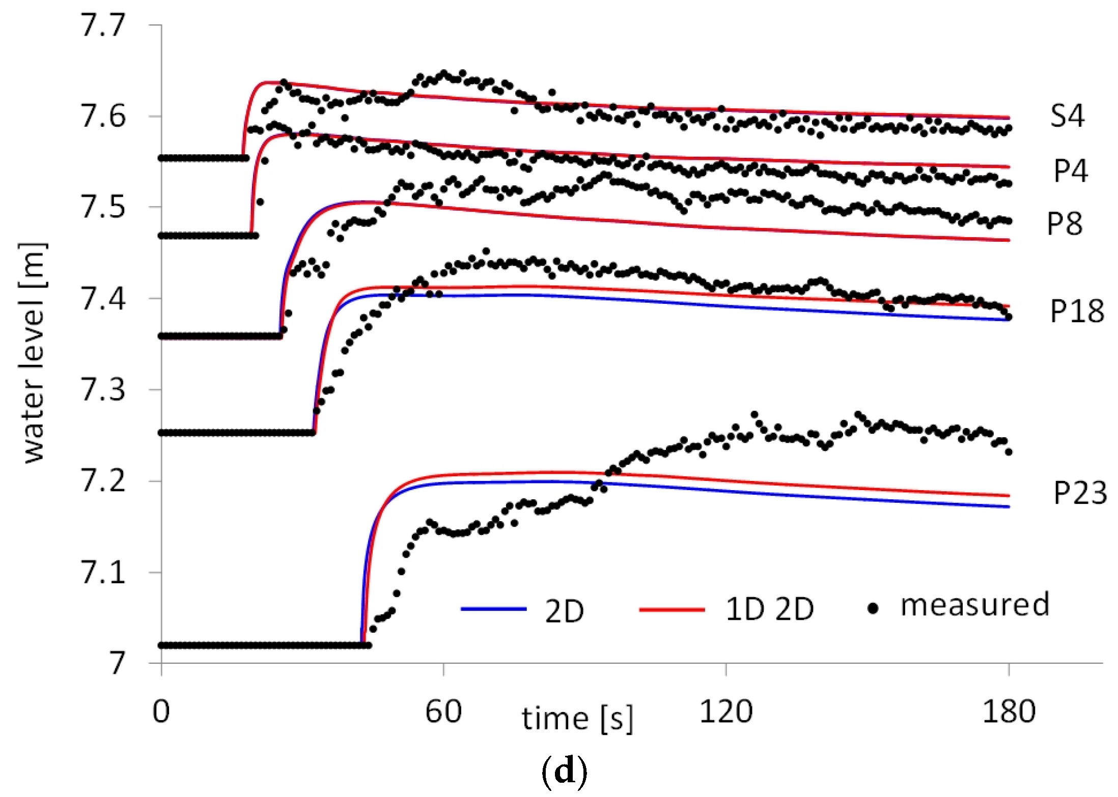
Figure 15a,b shows measured and computed water levels at some of the measure gauges for hydrograph HY1. In Figure 15a, we show also a comparison with the results obtained by a fully-dynamic shallow water model solved using a discontinuous Galerkin scheme [25]. Results computed by FLO over the coupled and 2D mesh show similar values and are in fairly good agreement with measured values. Measured values are closer to the FLO results in P13 and are closer to the results of the reference model in P21 and P26. Results of the proposed model show generally a wave front steeper than the measured one, likely due to the lack of inertial terms in the momentum equation. Observe that the results of the reference models are reported by the authors only in gauges with a regular change of the water level. In the gauges selected for the comparison of Figure 15b, the irregularity of the water levels would make the accuracy attained by the two models almost equivalent. Similar trends can be observed in the results of hydrograph HY2, shown in Figure 15c,d.

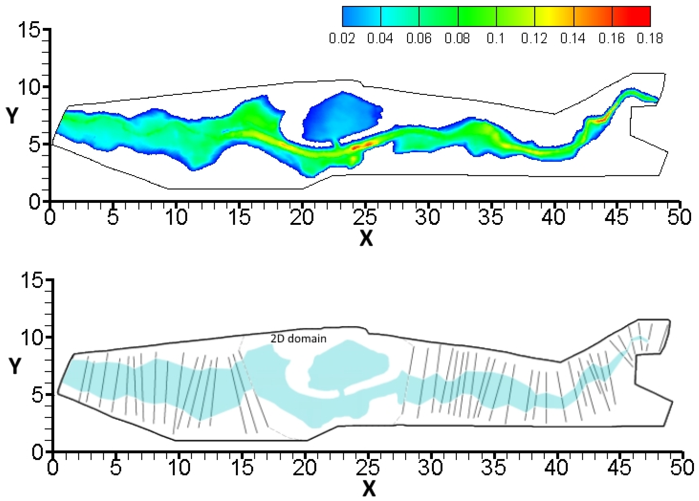
Figure 16 and Figure 17 show the flooded areas for simulation times of 60 s, for the two inflow hydrographs, computed by FLO over the two meshes. Very small differences can be observed among the flooded areas computed over the 2D and the 1D-2D meshes, with a maximum scatter of the order of 2%. Moreover, observe that the flooding arrival times computed over the 2D mesh are slightly less than the ones of the coupled mesh, because of the higher flow resistance in the 1D channel (see the results in Gauges P21 and P26).

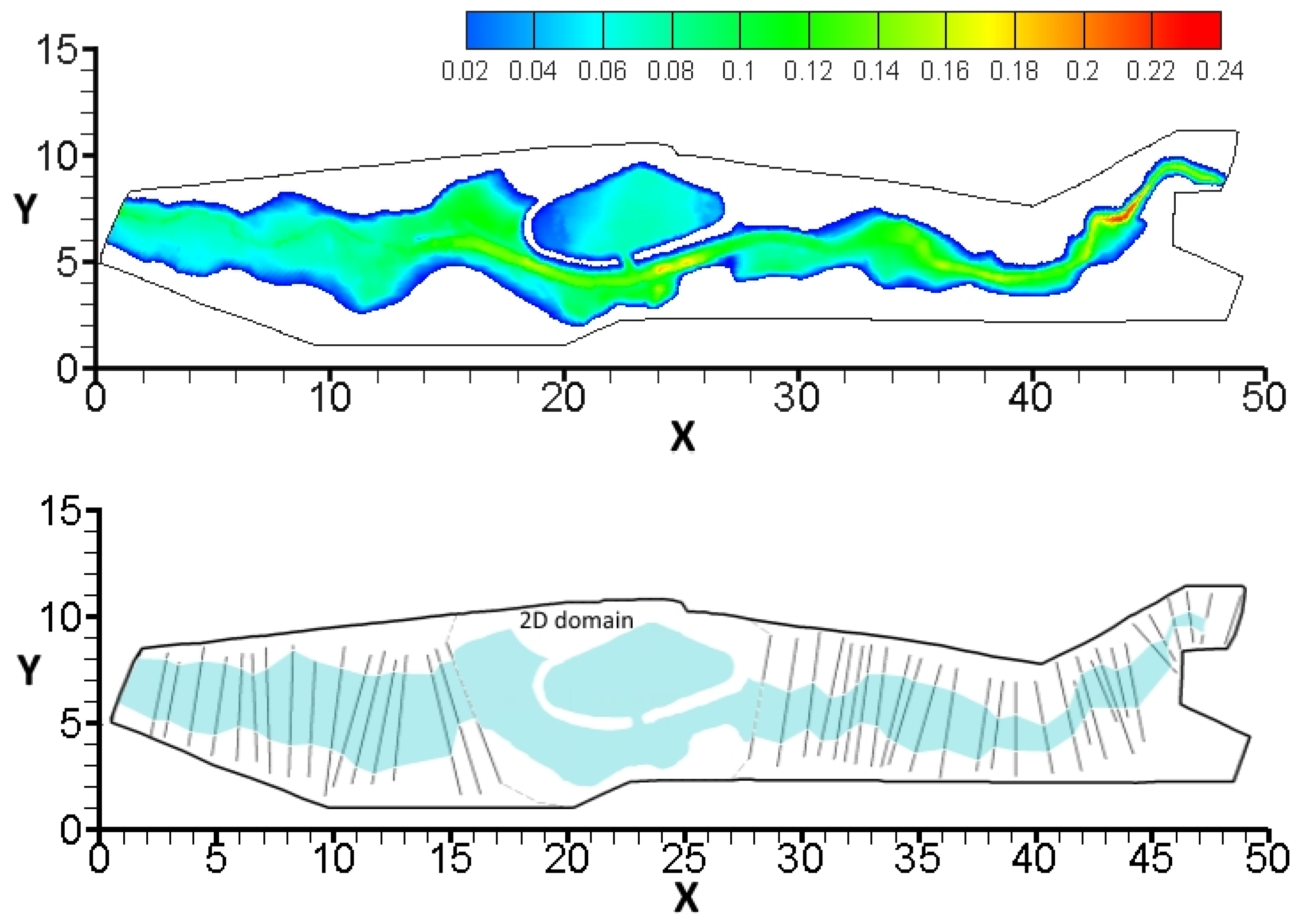
12. The Severn River (U.K.) Test Case

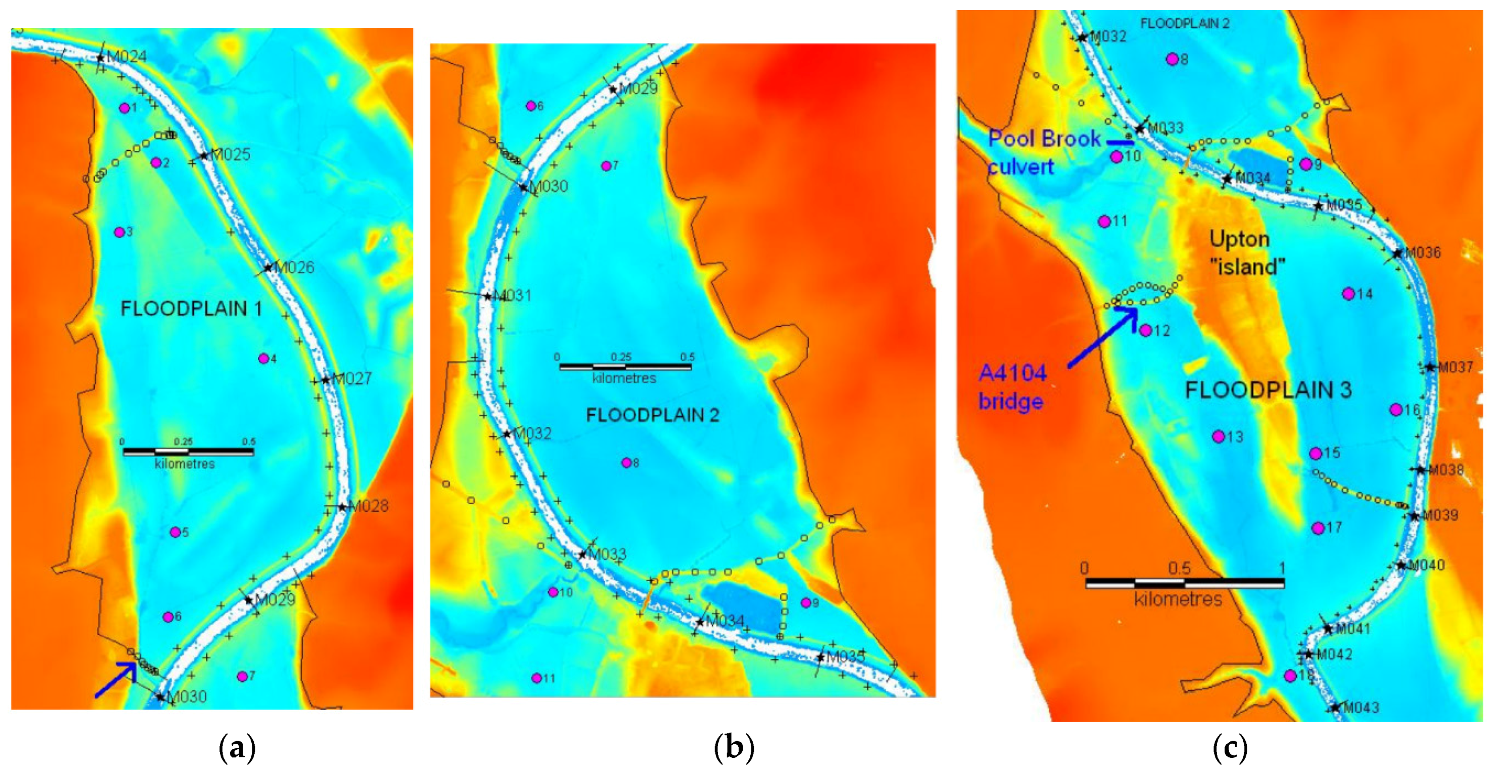
This test case has been proposed in the Benchmarking of 2D Hydraulic Modelling Packages during the joint Defra/Environment Agency research program [27,28] to evaluate the capability of several numerical codes to simulate fluvial flooding in a relatively large river, with flooding taking place as the result of river bank overtopping [27,28]. The site is approximately 7 km long, by 0.75–1.75 km wide with a set of three distinct floodplains (see Figure 18a,c) located in the proximity of the Upton-upon-Severn village (U.K.). The floodplains are not connected to each other.

River bank elevations with respect to the bottom bed vary between 13 m at the top end of Floodplain 1 (near Section M024), to 11.5 m at the bottom end of Floodplain 3 (just upstream of Section M044). During flooding, water poured down into the south end of Floodplain 1 for any river level higher than 10 m through the 10 m-wide opening close to Section M030. Water passed through the Pool Brook culvert (near Section M033) into Floodplain 3 at all times, but a level of ~10.5 m or higher was required for any significant flooding to happen [27,28].

A DEM with definition 1 m² and 42 1D sections profiles have been provided, with sections labelled from M013–M054 [27,28]. Uniform roughness has been assumed inside the channel and floodplains, equal respectively to n = 0.028 s/m^1/3 and n = 0.04 s/m^1/3 [27,28]. According to the topography of the studied area [27,28], the modelled flood is not expected to inundate roads and built-up areas to any significant extent. Therefore, a uniform roughness value has been used. Any effect of buildings has been neglected, as well as any head losses due to the river axis curvature [27,28].

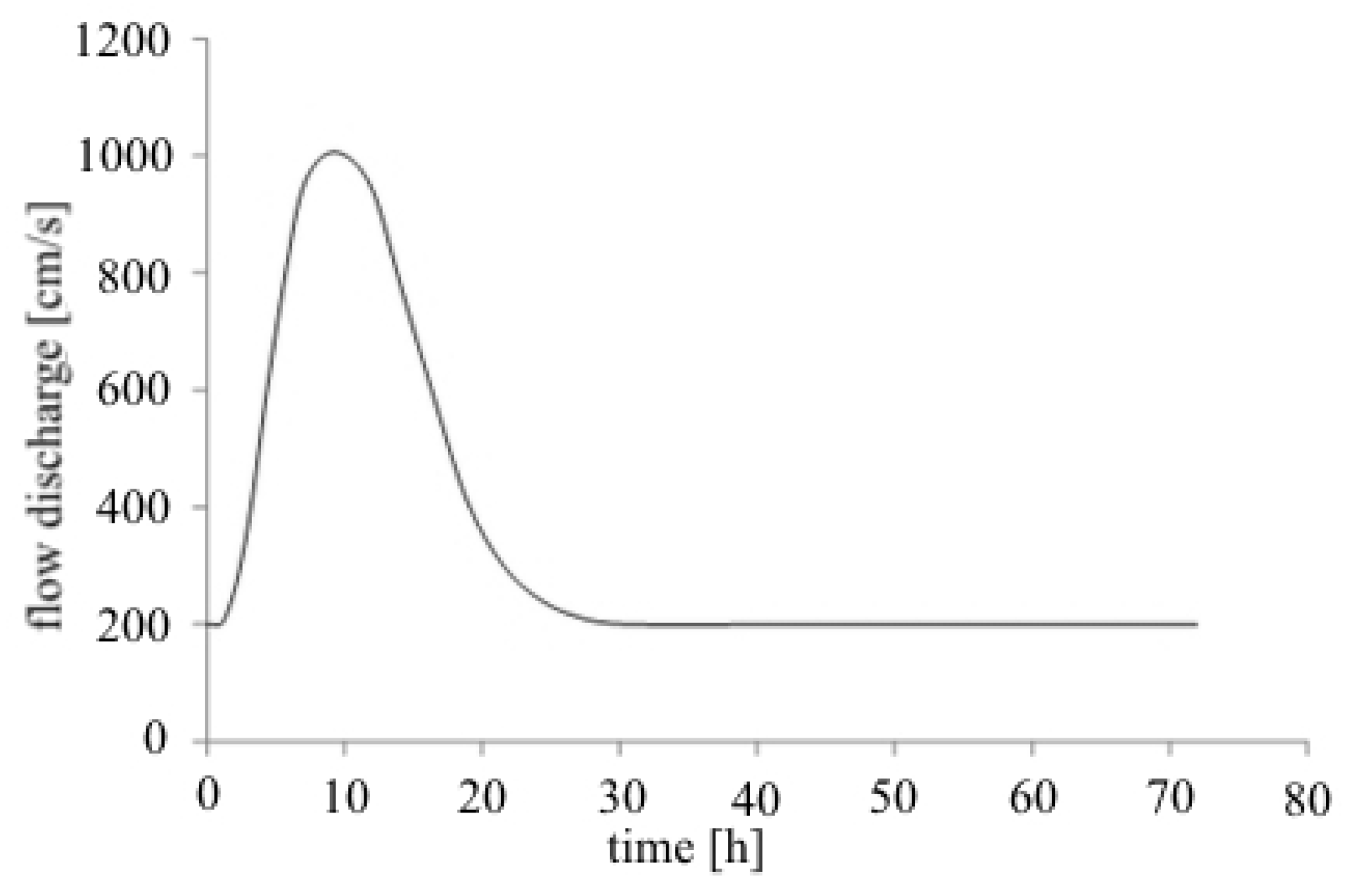
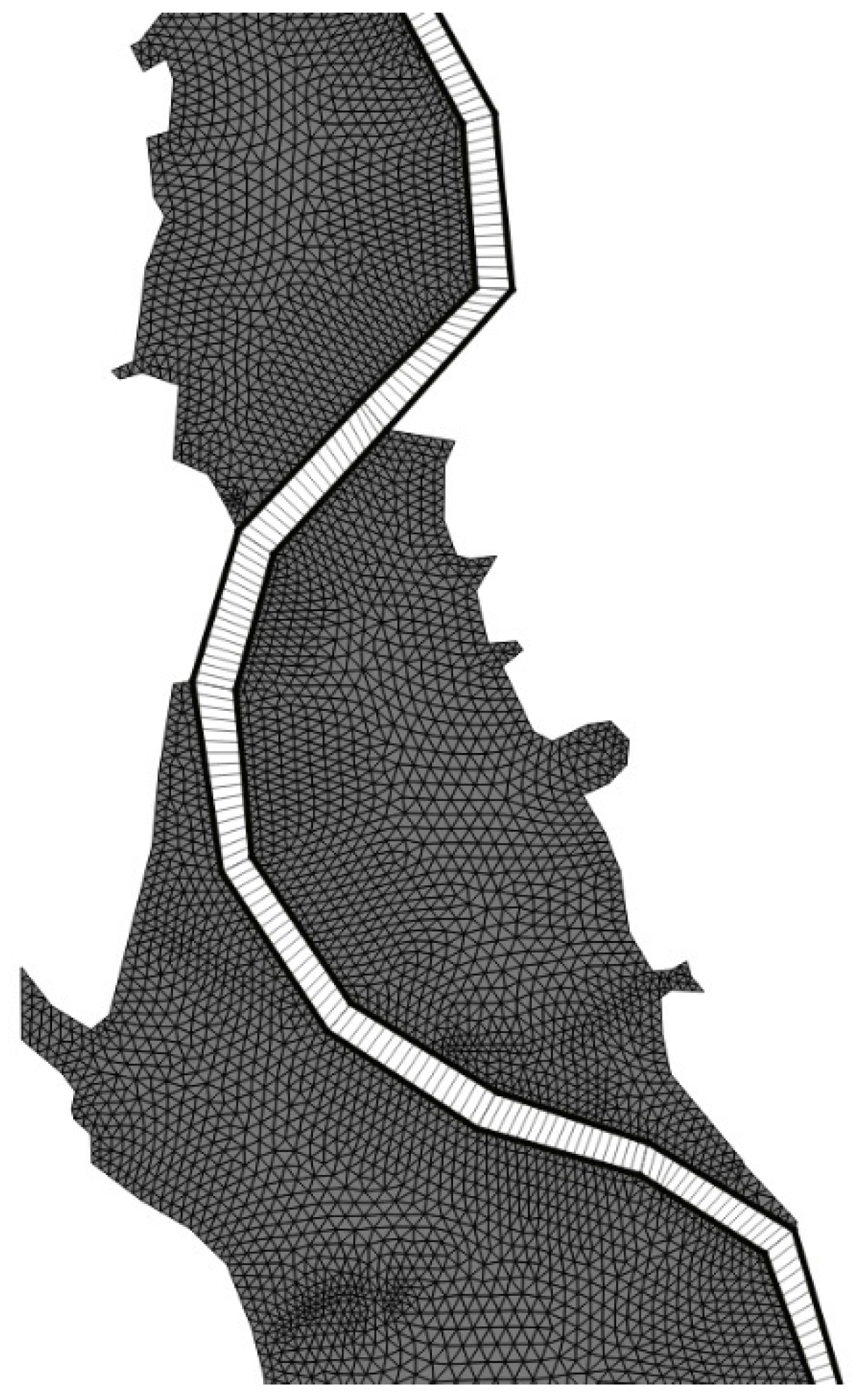
A 1D-2D mesh with lateral coupling, with 9842 triangles, 6271 nodes and 670 1D sections (42 measured) has been used in the FLO model (see Figure 19). The total simulation time is T = 72 h. The time step size is Δt = 10 s. At the upstream boundary (Section M013), an inflow discharge versus time has been applied (see Figure 20). A known rating curve has been applied at the downstream boundary in Cross-section M054. A uniform initial water level of 9.8 m has been assumed over all of the domain [27,28]. The maximum value of the CFL number is 7.9 in 2D floodplains and 1.34 in 1D channels. A fully-2D mesh has not been arranged, due to the missing data in the provided DEM of the river area.

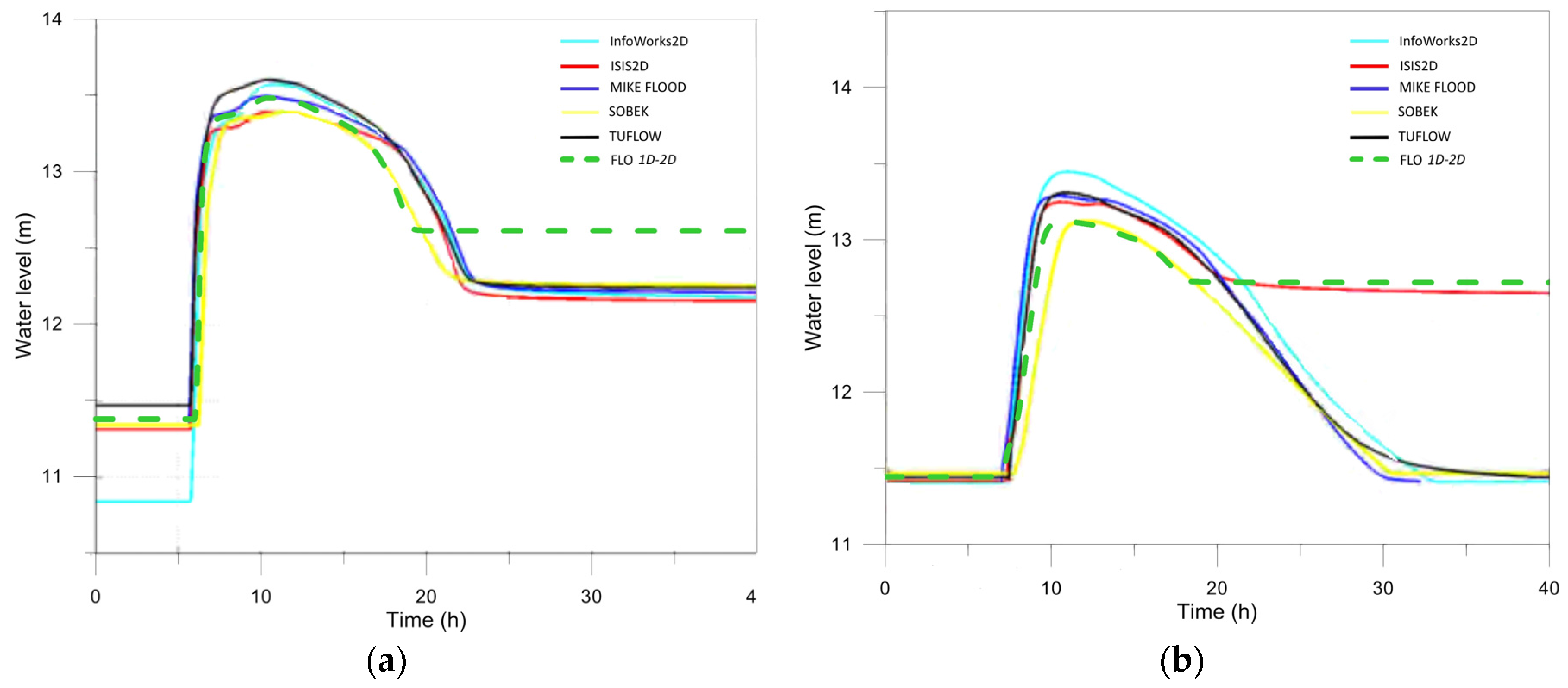
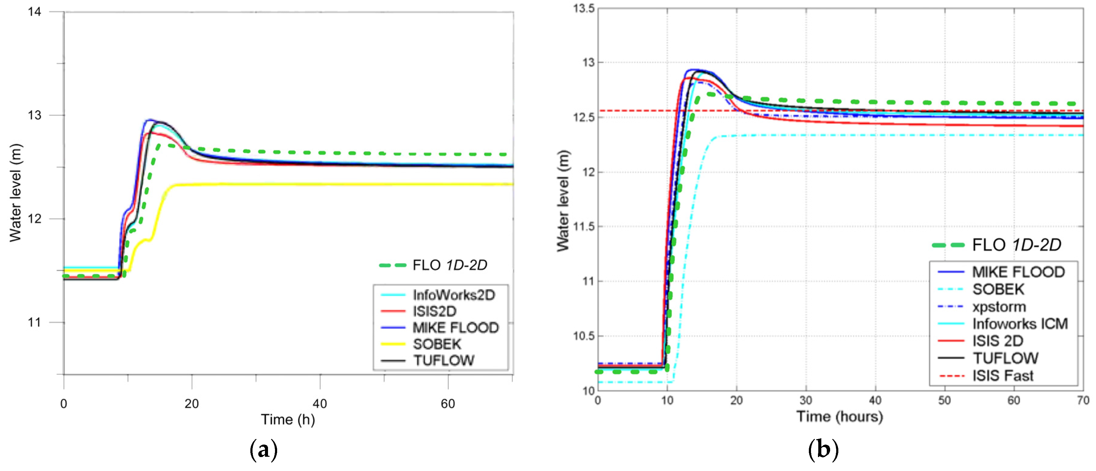
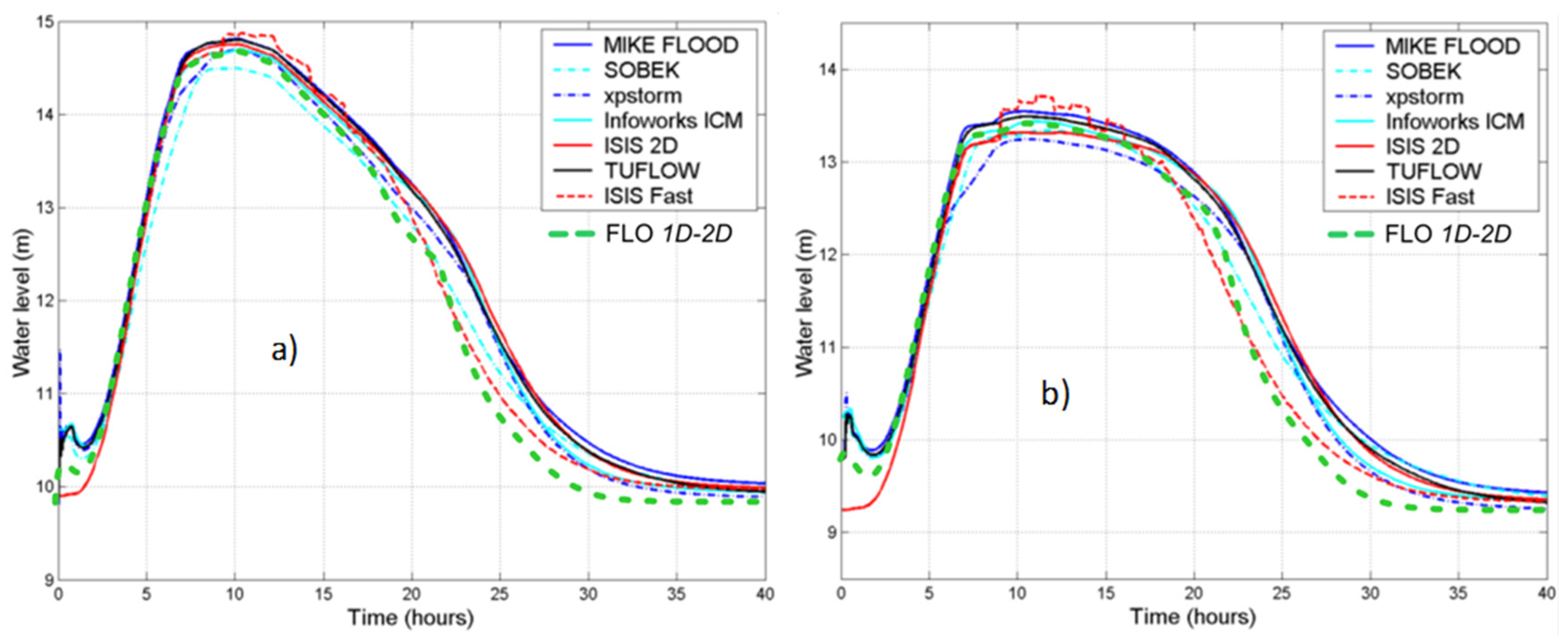
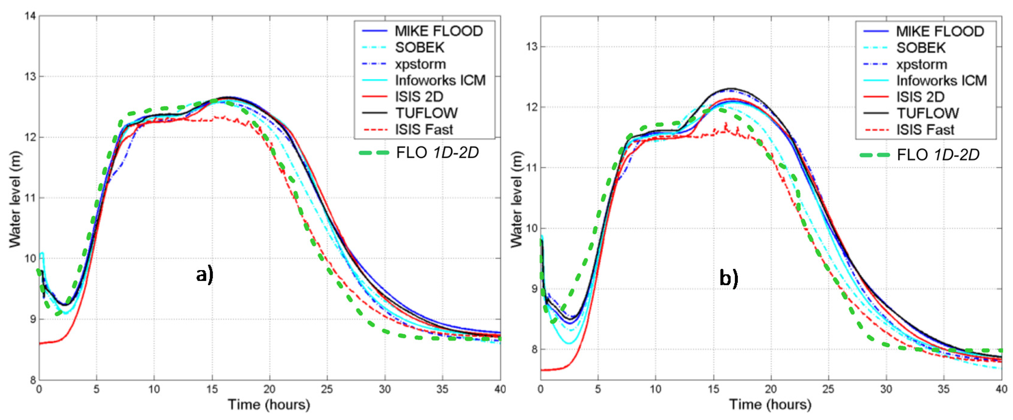
Figure 21a and Figure 22b show the computed water levels at four 1D channel sections. The predicted peak levels are in good agreement with the literature ones, especially in the first three sections, where the computed values are intermediate among the others, with maximum scatter 0.06 m. In Section M045 (in Figure 22b), the computed peak level is in agreement with the ones computed by SOBEK and MIKE, about 0.2 m below the other reference ones.

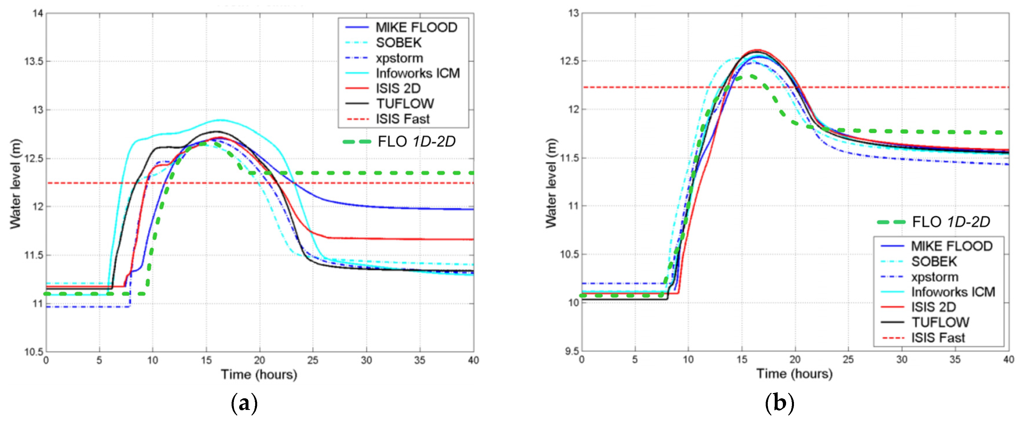
Figure 23a and Figure 25b show the computed water levels at different gauges in the three floodplains. Gauge 1 (in Figure 23a) lies in a low depression in an area of Floodplain 1 not protected by flood embankments. Predicted peak levels and arrival times are in agreement among all of the models and consistent with the 1D predictions at nearby river cross-sections (e.g., Section M025 in Figure 21b). Relative differences in computed peak levels are generally due to different approaches in the literature models used for (1) computation of discharges from river bank overtopping (which may include crucial parameters, such as discharge coefficients, etc.); (2) interpolation of the measured embankment crest elevations, whose minimum value occurring around flat areas is very similar to the hydrostatic maximum level.

Dewatering of the area close to Gauge 1 may occur only from the river side, in the reach between Sections M024–M025, due to a street close to Cliffey Wood (circled dots between Gauges 1 and 2 in Figure 20a) with topographic elevation higher than 13 m. The final level after dewatering is expected to be equal to ~12.13 m, the level of the lowest point along the river bank break line provided as part of the Test 7 dataset. All models predicted this level reasonably well, except ISIS 2D.

In the remaining part of Floodplain 1 (Gauges 2–6; here for simplicity, only Gauge 4 is shown in Figure 23b), predicted arrival times are very similar, and peak values are a bit smaller than the average values of the other models. Observe, during the dewatering phase, the difference between the water levels predicted by FLO and ISIS models and the other literature models. This is likely due to the fact that the 10-m opening near Cross-section M030, missing in the FLO and ISIS input data and marked by a row in the map of Figure 18a, has been modelled by the other codes. With the proposed and the ISIS models, levels decrease back to the lowest level along the embankment (12.72 m), which is correctly predicted.

At Gauges 7 and 8 (in Figure 24a,b), in Floodplain 2, all models, except SOBEK, predict the floodplain level to rise above the embankment elevations (~12.50 m) and to become controlled by river levels.

Gauges 10 and 11 in Floodplain 3 (here, only Gauge 11 is shown in Figure 25a) lie in the west area of Upton-upon-Severn village. Here, flood levels are expected to be similar to those in the river, with a rapid response due to the very large culvert allowing the Pool Brook (not modelled) to flow into the Severn. However, it is observed that the flood is predicted by the models to reach Gauge 11 with very large discrepancies in timing (up to 3 h). SOBEK, TUFLOW and InfoWorks ICM predict an earlier arrival than ISIS 2D, XPSTORM and MIKE FLOOD. A delay of the predicted flood time by FLO is observed with respect to SOBEK, TUFLOW, as well as to InfoWorks and ISIS, but the same delay is very small with respect to MIKE. Water level during the recession phase predicted by the FLO model is aligned to the one provided by MIKE (~12 m).

Gauges 12–17 (here, only the results of Gauge 14 are shown in Figure 25b) lie in Floodplain 3 (east of Upton-upon-Severn village). The floodplain has a small internal convexity immediately downstream of Upton Island and, due to the lack of any embankment along the river, is not defended against floods. Predicted peak levels in the floodplain are underestimated with respect to the reference models, while the final values after recession are well predicted (~11.51 m). The arrival flood times are in agreement with the other models, except SOBEK, which anticipates ~2.5 hours. Differences in the peak level with respect to the literature models could be due to the diffusive hypotheses.

13. Conclusions

A novel coupling 1D-2D strategy has been proposed in the shallow water models’ framework. Governing equations are written in diffusive form and solved in the water level unknown. The procedure deals with both lateral and frontal 1D-2D domain connection. Previously proposed coupling approaches, developed from previous existing 1D and 2D models, require specific operations, depending on how each model perceives the coupling with the other one. These operations can lead to severe restriction of numerical stability and result accuracy. The proposed approach does not require the solution of boundary equations nor an additional variable at 1D-2D interfaces. Computational cells in the 2D domain are the Voronoi polygons around each node, while standard 1D computational cells are the quadrilateral elements surrounding each section. Mixed cells include 1D computational cells and the Voronoi polygons of the 2D nodes located on the trace of the corresponding river section. In both the prediction and the correction steps, the same procedures are applied to solve computational cells, regardless if they are standard 2D, standard 1D or mixed cells.

The efficiency of the coupling model is tested throughout several examples, both academic and real-world applications. Good agreement has been found with measured data and literature results, with the advantages of the diffusive model related to computational efficiency and robustness previously discussed in the Introduction. These advantages become more and more important along with the complexity of the source terms estimated in the continuity equations, according to actual hydrologic transformation and soil interactions [29].