
Response of Hydrological Processes to Input Data in High Alpine Catchment: An Assessment of the Yarkant River basin in China


Abstract
:1. Introduction
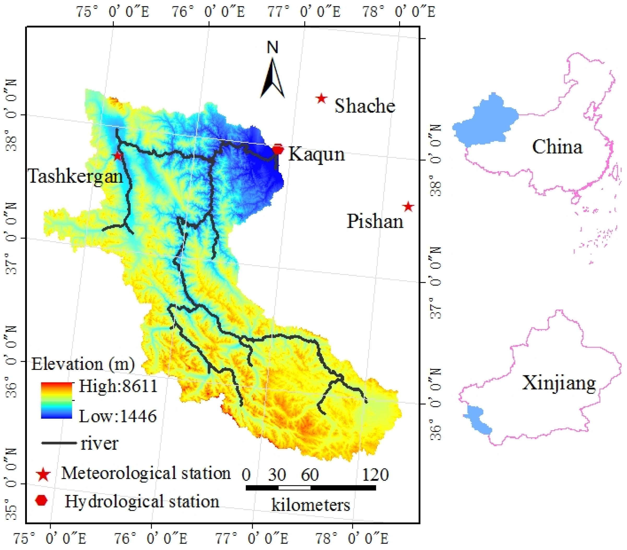
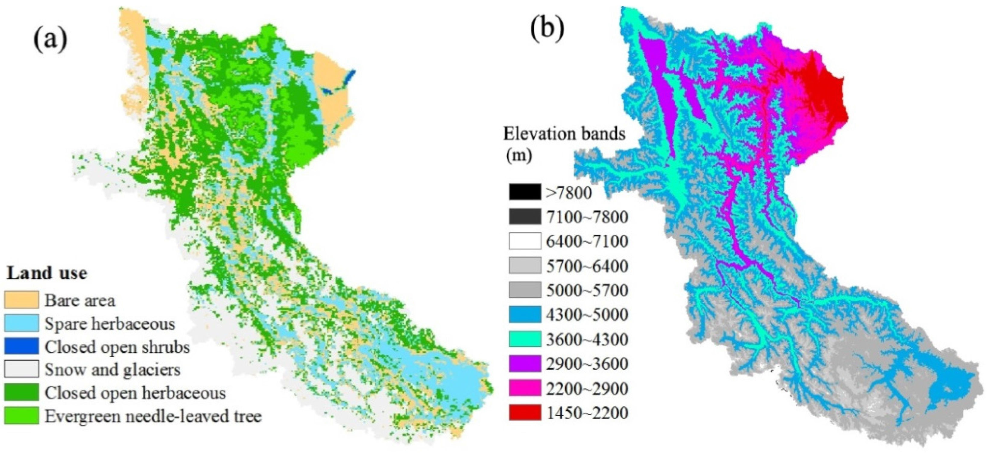
2. Study Area
3. Forcing Data
3.1. Station Data
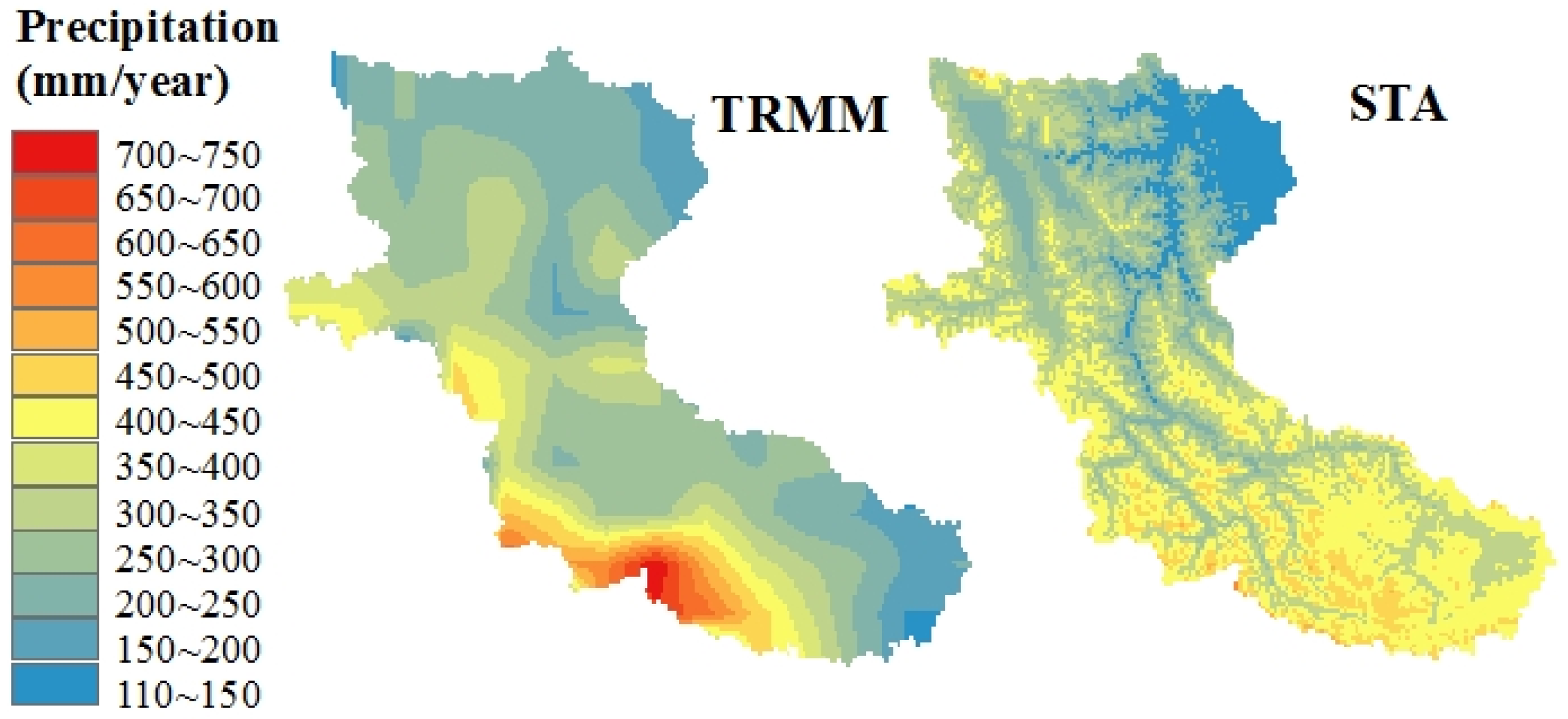
3.2. TRMM
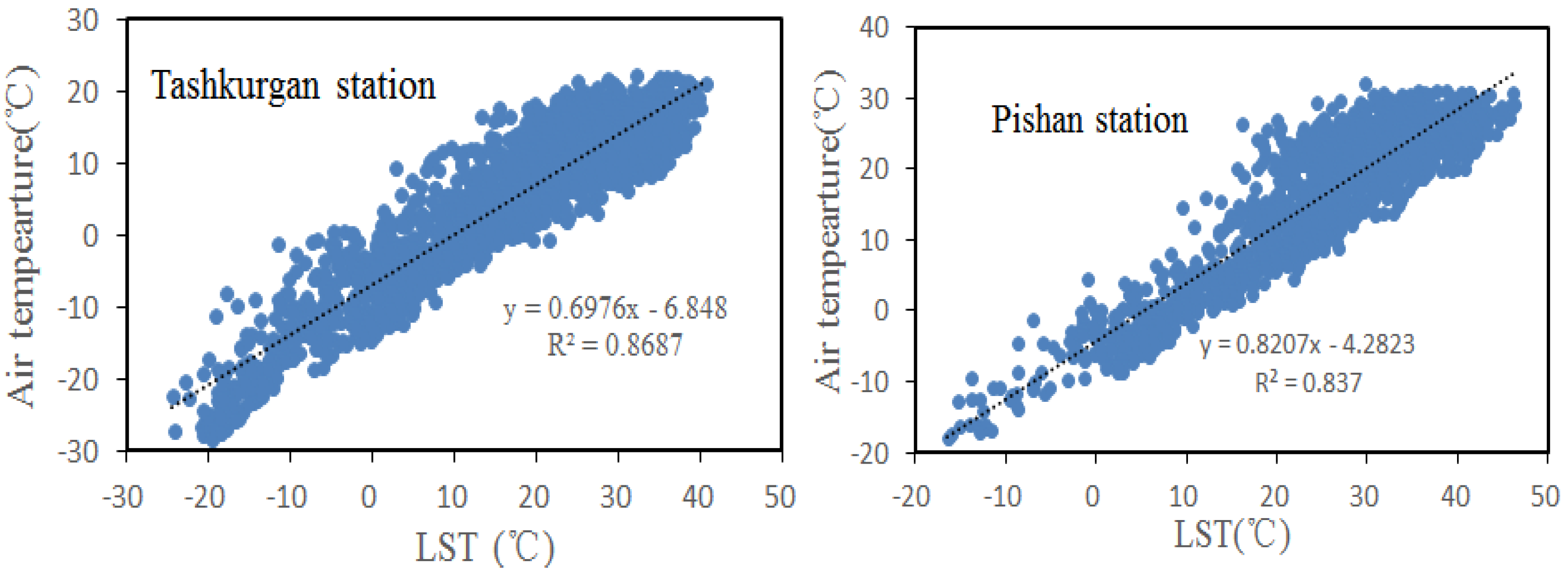
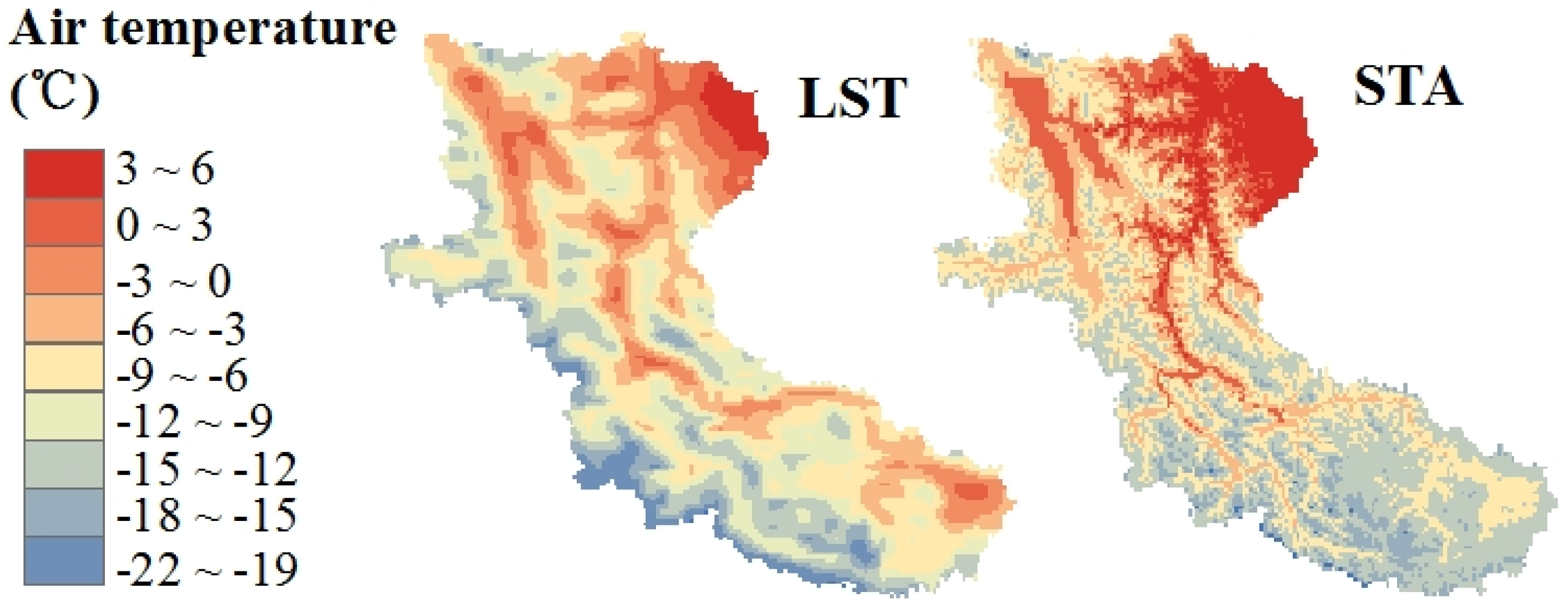
3.3. LST
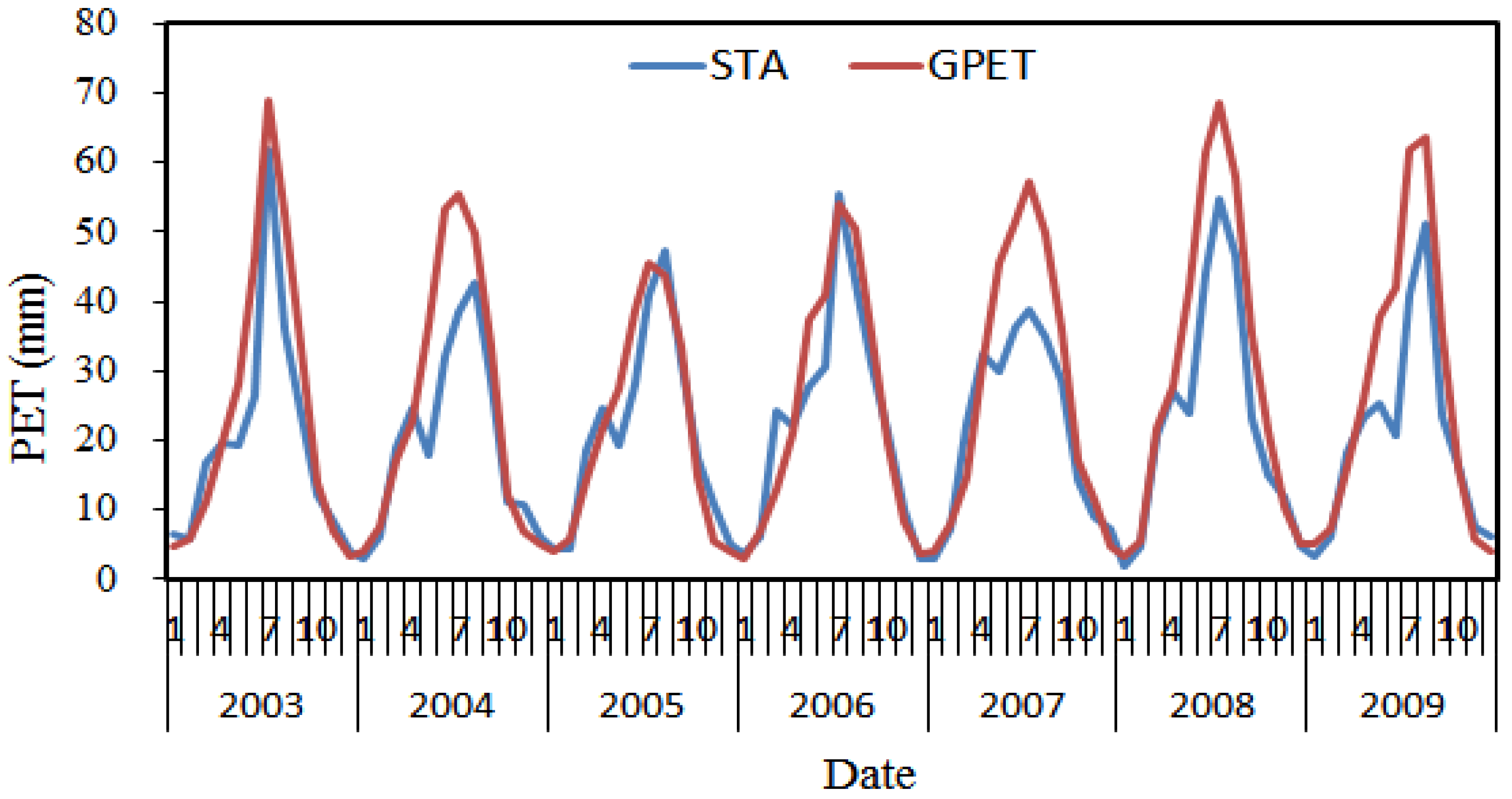
3.4. PET
4. Methodology
4.1. Models
4.2. Calibration
4.3. Hypothesis Test
5. Results and Discussion
5.1. Simulated Discharges
5.2. Sensitivities of Water Components
5.3. Responses of Hydrological Processes
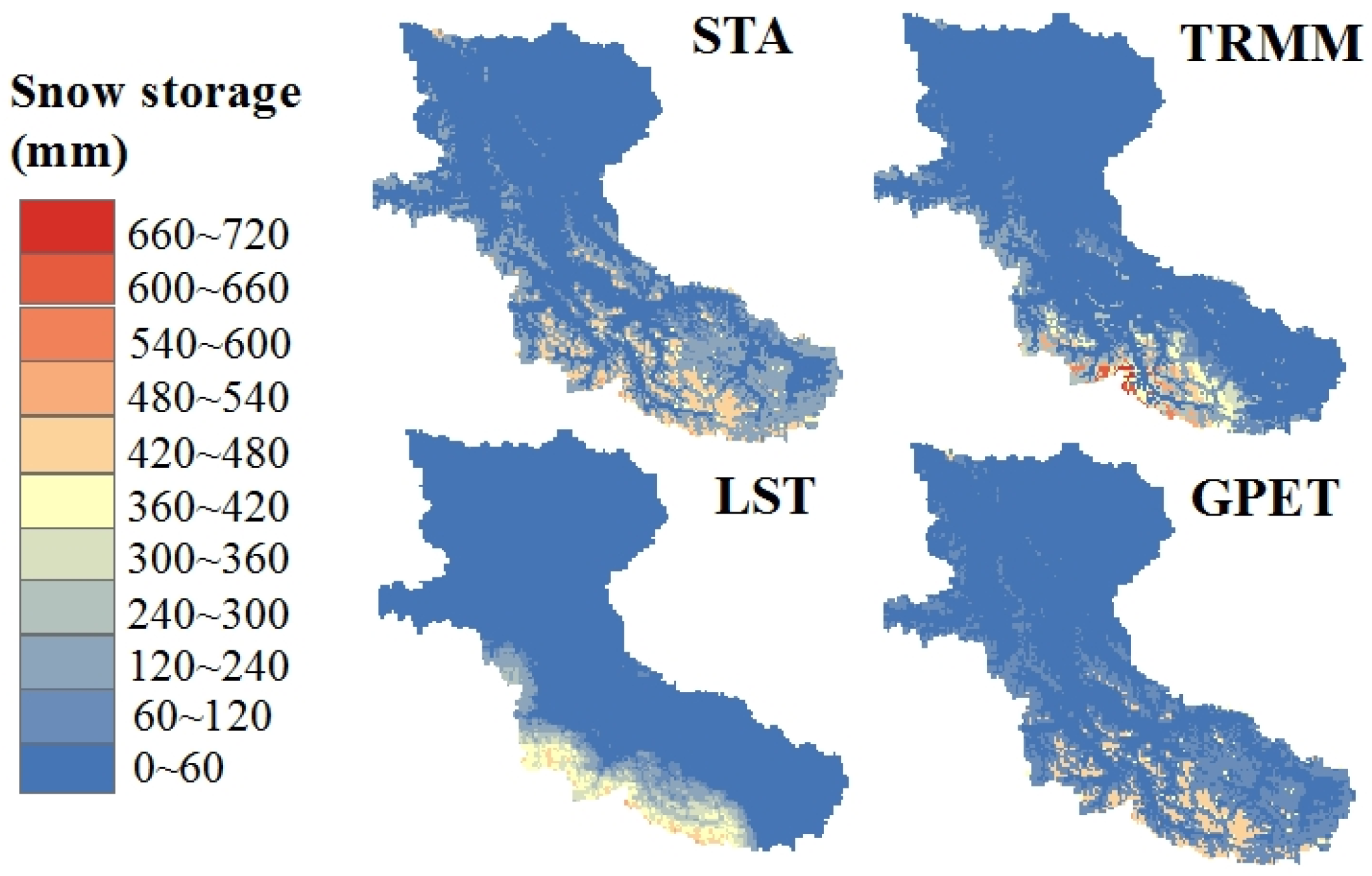
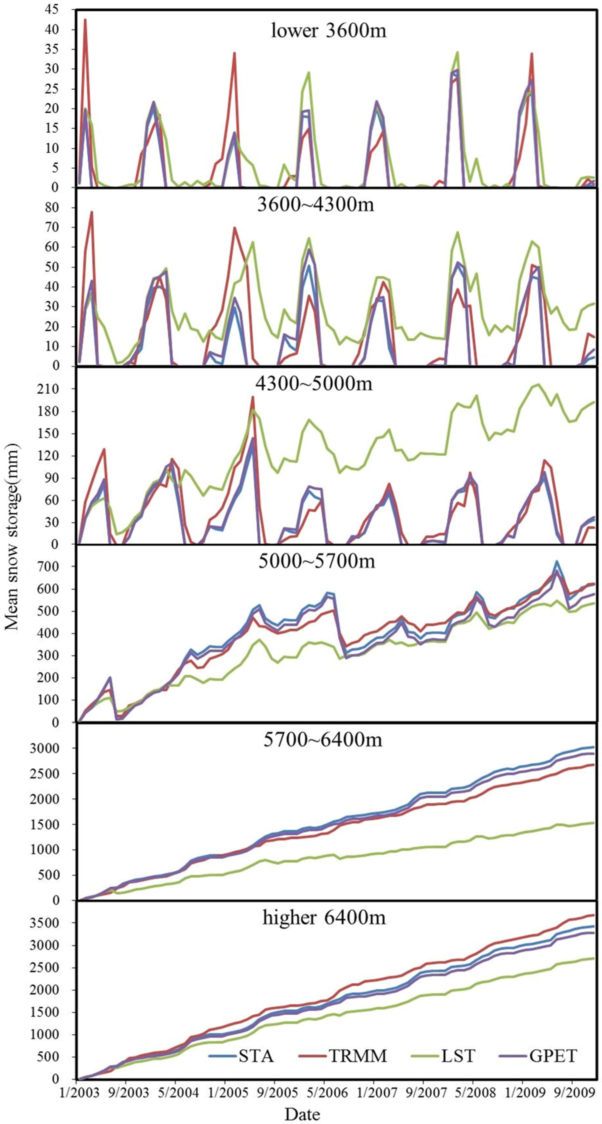
5.3.1. Snow Storage
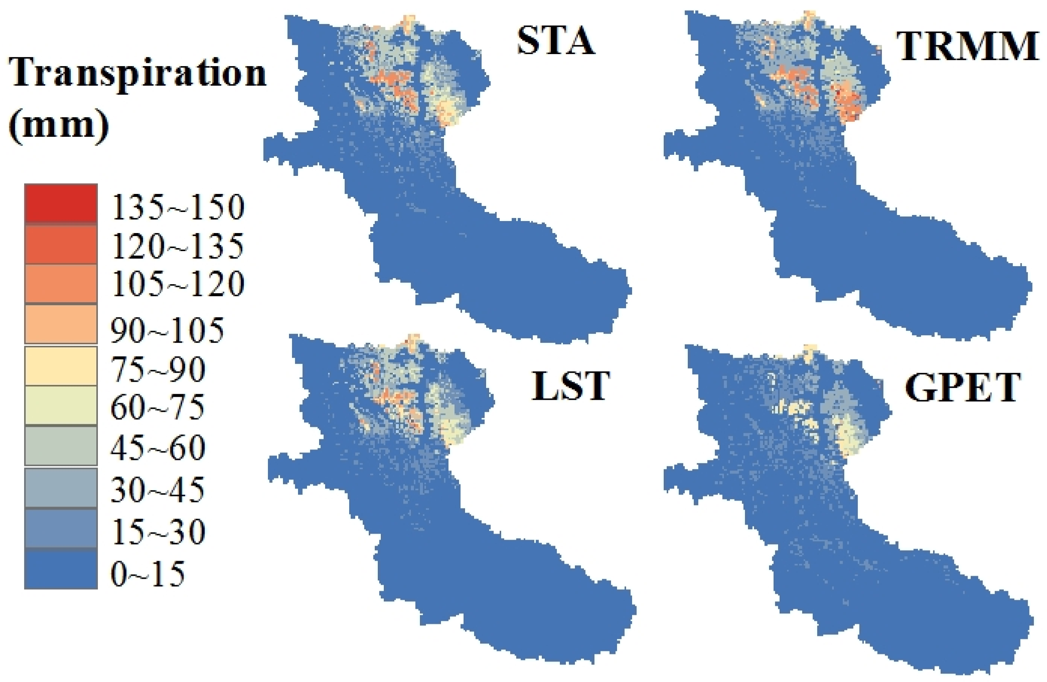
5.3.2. Plant Transpiration
6. Conclusions
Acknowledgments
Author Contributions
Conflicts of Interest
References
- Beven, K.; Binley, A. The future of distributed models: Model calibration and uncertainty prediction. Hydrol. Process. 1992, 6, 279–298. [Google Scholar] [CrossRef]
- Jasper, A.V.; Hoshin, V.G.; Willem, B.; Soroosh, S. A Shuffled Complex Evolution Metropolis algorithm for optimization and uncertainty assessment of hydrologic model paremeters. Water Resour. Res. 2003, 39, 1–16. [Google Scholar]
- Misgana, K.M.; John, W.N. Sensitivity and uncertainty analysis coupled with automatic calibration for a distributed watershed model. J. Hydrol. 2005, 306, 127–145. [Google Scholar]
- Zhang, X.S.; Raghavan, S.; David, B. Calibration and uncertainty analysis of the SWAT model using Genetic Algorithm and Bayesian Model Averaging. J. Hydrol. 2009, 374, 307–317. [Google Scholar] [CrossRef]
- Jin, X.L.; Xu, C.Y.; Zhang, Q.; Singh, V.P. Parameter and modeling uncertainty simulated by GLUE and a formal Bayesian method for a conceptual hydrological model. J. Hydrol. 2010, 383, 147–155. [Google Scholar] [CrossRef]
- Ajami, N.K.; Duan, Q.; Gao, X.; Soroosh, S. Multimodel combination techniques for analysis of hydrological simulations application to distributed model intercomparison project results. J. Hydrometeorol. 2006, 4, 755–768. [Google Scholar] [CrossRef]
- Ajami, N.K.; Duan, Q.; Sorooshian, S. An integrated hydrologic Bayesian multimodel combination framework: Confronting input, parameter, and model structural uncertainty in hydrologic prediction. Water Resour. Res. 2007, 43, 1–10. [Google Scholar]
- Kavetski, D.; Kuczera, G.; Franks, S.W. Bayesian analysis of input uncertainty in hydrological modeling: 2. Application. Water Resour. Res. 2006, 42, 1–9. [Google Scholar] [CrossRef]
- Xu, C.Y.; Tunemar, L.; Chen, Y.D.; Singh, V.P. Evaluation of seasonal and spatial variations of lumped water balance model sensitivity to precipitation data errors. J. Hydrol. 2006, 324, 80–93. [Google Scholar] [CrossRef]
- Thompson, J.R.; Green, A.J.; Kingston, D.G. Potential evapotranspiration-related uncertainty in climate change impacts on river flow: An assessment for the Mekong River basin. J. Hydrol. 2014, 510, 259–279. [Google Scholar] [CrossRef]
- Dobler, C.; Bürger, G.; Stötter, J. Assessment of climate change impacts on flood hazard potential in the Alpine Lech watershed. J. Hydrol. 2012, 460, 29–39. [Google Scholar] [CrossRef]
- Chien, H.; Yeh, P.J.; Knouft, J.H. Modeling the potential impacts of climate change on streamflow in agricultural watersheds of the Midwestern United States. J. Hydrol. 2013, 491, 73–88. [Google Scholar] [CrossRef]
- Xu, Y.P.; Zhang, X.; Ran, Q.; Tian, Y. Impact of climate change on hydrology of upper reaches of Qiantang River Basin, East China. J. Hydrol. 2013, 483, 51–60. [Google Scholar] [CrossRef]
- Zhang, X.; Xu, Y.P.; Fu, G. Uncertainties in SWAT extreme flow simulation under climate change. J. Hydrol. 2014, 515, 205–222. [Google Scholar] [CrossRef]
- Blazkova, S.; Beven, K. Flood frequency estimation by continuous simulation for a catchment treated as ungauged (with uncertainty). Water Resour. Res. 2002, 38, 1411–1414. [Google Scholar] [CrossRef]
- Stisen, S.; Jensen, K.H.; Sandholt, I.; Grimes, D.I. A remote sensing driven distributed hydrological model of the Senegal River basin. J. Hydrol. 2008, 354, 131–148. [Google Scholar] [CrossRef]
- Liu, T.; Willems, P.; Feng, X.W.; Li, Q.; Huang, Y.; Bao, A.M.; Chen, X.; Veroustraete, F.; Dong, Q.H. On the usefulness of remote sensing input data for spatially distributed hydrological modelling: Case of the Tarim River basin in China. Hydrol. Process. 2012, 26, 335–344. [Google Scholar] [CrossRef]
- Sun, W.; Ishidaira, H.; Bastola, S. Calibration of hydrological models in ungauged basins based on satellite radar altimetry observations of river water level. Hydrol. Process. 2012, 26, 3524–3537. [Google Scholar] [CrossRef]
- Deus, D.; Gloaguen, R.; Krause, P. Water Balance Modeling in a Semi-Arid Environment with Limited in Situ Data Using Remote Sensing in Lake Manyara, East African Rift, Tanzania. Remote Sens. 2013, 5, 1651–1680. [Google Scholar] [CrossRef]
- Van, D.A. Model-data fusion: Using observations to understand and reduce uncertainty in hydrological models. In Proceedings of the 19th International Congress on Modelling and Simulation (MODSIM 2011), Perth, Australia, 12–16 December 2011.
- McMichael, C.E.; Hope, A.S.; Loaiciga, H.A. Distributed hydrological modelling in California semi-arid shrublands: MIKE SHE model calibration and uncertainty estimation. J. Hydrol. 2006, 317, 307–324. [Google Scholar]
- Knoche, M.; Fischer, C.; Pohl, E.; Krause, P.; Merz, R. Combined uncertainty of hydrological model complexity and satellite-based forcing data evaluated in two data-scarce semi-arid catchments in Ethiopia. J. Hydrol. 2014, 519, 2049–2066. [Google Scholar]
- Prigent, C. Precipitation retrieval from space: An overview. Comptes Rendus Geosci. 2010, 342, 380–389. [Google Scholar]
- Shi, Y.F. Brief of Glacier Inventory of China; Shanghai Popular Science Press: Shanghai, China, 2005. (In Chinese) [Google Scholar]
- Tang, H.; Yang, D.G.; Zhang, Y.F. Food security and agricultural structural adjustment in Yarkant River Basin, northwest China. J. Food Agricul. Environ. 2013, 11, 324–328. [Google Scholar]
- Gao, X.; Zhang, S.Q.; Ye, B.S.; Qiao, C.J. Glacier Runoff Change in the Upper Stream of Yarkant River and Its Impact on River Runoff during 1961–2006. J. Glaciol. Geocryol. 2010, 32, 445–453. (In Chinese) [Google Scholar]
- Liu, J.; Liu, T.; Bao, A.M.; Philippe, D.M.; Feng, X.W.; Scott, N.M.; Chen, X. Assessment of Different Modelling Studies on the Spitial Hydrological Processes in an Arid Alpine Catchment. Water Resour. Manag. 2016, 30, 1757–1770. [Google Scholar] [CrossRef]
- Huffman, G.J.; Adler, R.F.; Bolvin, D.T.; Gu, G.; Nelkin, E.J.; Bowman, K.P.; Hong, Y.; Stocker, E.F.; Wolff, D.B. The TRMM multisatellite precipitation analysis (TMPA): Quasi-global, multiyear, combined-sensor precipitation estimates at fine scales. J. Hydeometeorol. 2007, 8, 38–55. [Google Scholar] [CrossRef]
- Xuan, J.; Luo, Y. Quality Assessment of the TRMM Precipitation Data in Mid Tianshan Mountains. Arid Land Geogr. 2013, 36, 253–262. (In Chinese) [Google Scholar]
- Schmidli, J.; Frei, C.; Vidale, P.L. Downscaling from GCM precipitation: A benchmark for dynamical and statistical downscaling methods. Int. J. Climatol. 2006, 26, 679–689. [Google Scholar] [CrossRef]
- Hulley, G.C.; Hook, S.J. Intercomparison of versions 4, 4.1 and 5 of the MODIS Land Surface Temperature and Emissivity products and validation with laboratory measurements of sand samples from the Namib desert, Namibia. Remote Sens. Environ. 2009, 113, 1313–1318. [Google Scholar] [CrossRef]
- Vogt, J.V.; Viau, A.A.; Paquet, F. Mapping regional air temperature fields using satellite-derived surface skin temperatures. Int. J. Climato. 1997, 17, 1559–1579. [Google Scholar] [CrossRef]
- Cristóbal, J.; Ninyerola, M.; Pons, X. Modeling air temperature through a combination of remote sensing and GIS data. J. Geophy. Res. 2008, 113. [Google Scholar] [CrossRef]
- Allen, R.G.; Pereira, L.S.; Raes, D.; Smith, M. Crop Evapotranspiration-Guidelines for Computing Crop Water Requirements-FAO Irrigation and Drainage Paper 56; FAO: Rome, Italy, 1998; Volume 300, p. D05109. [Google Scholar]
- Abbott, M.; Bathurst, J.; Cunge, J.; O’connell, P.; Rasmussen, J. An introduction to the European Hydrological System-Systeme Hydrologique Europeen, “SHE”, 2: Structure of a physically-based, distributed modelling system. J. Hydrol. 1986, 87, 61–77. [Google Scholar] [CrossRef]
- Duan, Q.; Gupta, V.K.; Sorooshian, S. Shuffled complex evolution approach for effective and efficient global minimization. J. Optim. Theory Appl. 1993, 76, 501–521. [Google Scholar] [CrossRef]
- Nash, J.; Sutcliffe, J.V. River flow forecasting through conceptual models part I-A discussion of principles. J. Hydrol. 1970, 10, 282–290. [Google Scholar] [CrossRef]
- Michael, H.K.; Christopher, J.N.; John, N.; William, L. Applied Linear Statistical Models; McGraw-Hill Education: New York, NY, USA, 2005. [Google Scholar]
- Fabio, F.; Christian, R.; Tobias, J.; Gabriel, A.; Stefan, W. Alpine Grassland Phenology as Seen in AVHRR, VEGETATION, and MODIS NDVI Time Series-a Comparison with in Situ Measurement. Sensors 2008, 8, 2833–2853. [Google Scholar]
- Kristensen, K.J.; Jensen, S.E. A model for estimating actual evapotranspiration from potential evapotranspiration. Nordic Hydrol. 1975, 6, 170–188. [Google Scholar]


| Altitude Group (m) | PCG (mm/km/year) | TCG (°/km) |
|---|---|---|
| <3000 | 0.0 | −6.5 |
| 3000–5000 | −70.0 | −6.8 |
| 5000–7000 | 100.0 | −7.0 |
| >7000 | 70.0 | −6.8 |
| Station | Dr | Dw | Dw_0.3 | rraw | rcor |
|---|---|---|---|---|---|
| Tashkurgan | 0.54 | 0.75 | 0.95 | 0.11 | 0.45 |
| Shache | 0.21 | 0.87 | 0.96 | 0.67 | 0.77 |
| Pishan | 0.15 | 0.88 | 0.99 | 0.36 | 0.67 |
| Data Source | Model Abbreviation | ||
|---|---|---|---|
| Rainfall | Temperature | Evapotranspiration | |
| station | station | station | STA |
| TRMM | station | station | TRMM |
| station | LST | station | LST |
| station | station | GPET | GPET |
| TRMM | LST | station | TRLS |
| TRMM | station | GPET | TRGP |
| station | LST | GPET | LSGP |
| TRMM | LST | GPET | RSD |
| Models | STA | TRMM | LST | GPET | TRLS | TRGP | LSGP | RSD |
|---|---|---|---|---|---|---|---|---|
| DDF (mm/day/°C) | 2.01 | 2.03 | 1.25 | 1.98 | 1.25 | 2.00 | 1.23 | 1.25 |
| TMT (°C) | −0.98 | −1.00 | −0.56 | −1.01 | −0.57 | −1.02 | −0.56 | −0.55 |
| LAI_NLT * | 3.81 | 3.82 | 3.78 | 2.65 | 3.82 | 2.64 | 2.63 | 2.66 |
| RD_NLT (mm) * | 4500 | 4500 | 4500 | 4000 | 4500 | 4000 | 4000 | 4000 |
| Model | STA | TRMM | LST | GPET | TRLS | TRGP | LSGP | RSD |
|---|---|---|---|---|---|---|---|---|
| NSC | 0.65 | 0.50 | 0.52 | 0.61 | 0.55 | 0.42 | 0.52 | 0.46 |
| R | 0.84 | 0.73 | 0.75 | 0.81 | 0.74 | 0.68 | 0.74 | 0.70 |
| RMSE | 172.10 | 207.15 | 204.49 | 183.52 | 197.35 | 222.81 | 204.11 | 214.66 |
| Groups | A | B | C | A*B | A*C | B*C | A*B*C |
|---|---|---|---|---|---|---|---|
| OLF | 0.000 | 0.221 | 0.691 | 0.040 | 0.714 | 0.399 | 0.336 |
| BF | 0.003 | 0.436 | 0.008 | 0.087 | 0.619 | 0.450 | 0.553 |
| SS | 0.003 | 0.000 | 0.945 | 0.001 | 0.828 | 0.415 | 0.430 |
| SNOWS | 0.271 | 0.000 | 0.224 | 0.789 | 0.546 | 0.120 | 0.282 |
| CI | 0.000 | 0.000 | 0.000 | 0.007 | 0.089 | 0.028 | 0.431 |
| WE | 0.000 | 0.000 | 0.000 | 0.937 | 0.085 | 0.072 | 0.573 |
| SOILE | 0.138 | 0.238 | 0.000 | 0.747 | 0.241 | 0.739 | 0.932 |
| PT | 0.541 | 0.535 | 0.000 | 0.751 | 0.637 | 0.809 | 0.905 |
© 2016 by the authors; licensee MDPI, Basel, Switzerland. This article is an open access article distributed under the terms and conditions of the Creative Commons Attribution (CC-BY) license (http://creativecommons.org/licenses/by/4.0/).
Share and Cite
Liu, J.; Liu, T.; Bao, A.; De Maeyer, P.; Kurban, A.; Chen, X. Response of Hydrological Processes to Input Data in High Alpine Catchment: An Assessment of the Yarkant River basin in China. Water 2016, 8, 181. https://doi.org/10.3390/w8050181
Liu J, Liu T, Bao A, De Maeyer P, Kurban A, Chen X. Response of Hydrological Processes to Input Data in High Alpine Catchment: An Assessment of the Yarkant River basin in China. Water. 2016; 8(5):181. https://doi.org/10.3390/w8050181
Chicago/Turabian StyleLiu, Jiao, Tie Liu, Anming Bao, Philippe De Maeyer, Alishir Kurban, and Xi Chen. 2016. "Response of Hydrological Processes to Input Data in High Alpine Catchment: An Assessment of the Yarkant River basin in China" Water 8, no. 5: 181. https://doi.org/10.3390/w8050181
APA StyleLiu, J., Liu, T., Bao, A., De Maeyer, P., Kurban, A., & Chen, X. (2016). Response of Hydrological Processes to Input Data in High Alpine Catchment: An Assessment of the Yarkant River basin in China. Water, 8(5), 181. https://doi.org/10.3390/w8050181