Article

Exploring the Non-Stationary Effects of Forests and Developed Land within Watersheds on Biological Indicators of Streams Using Geographically-Weighted Regression

1
Department of Environmental Planning, Konkuk University, 120 Neungdong-ro, Kwangjin-gu, Seoul 05029, Korea
2
Department of Environmental Health Science, Konkuk University, 120 Neungdong-ro, Kwangjin-gu, Seoul 05029, Korea
3
Landscape Ecological Lab, Department of Environmental Planning, Konkuk University, 120 Neungdong-ro, Kwangjin-gu, Seoul 05029, Korea
4
Gyeonggi Research Institute, 1128 Gyeongsu-daero, Suwon, Gyeonggi-do 16207, Korea
*
Author to whom correspondence should be addressed.
Water 2016, 8(4), 120; https://doi.org/10.3390/w8040120
Submission received: 15 December 2015 / Revised: 16 February 2016 / Accepted: 23 March 2016 / Published: 28 March 2016

Abstract

:
This study examined the non-stationary relationship between the ecological condition of streams and the proportions of forest and developed land in watersheds using geographically-weighted regression (GWR). Most previous studies have adopted the ordinary least squares (OLS) method, which assumes stationarity of the relationship between land use and biological indicators. However, these conventional OLS models cannot provide any insight into local variations in the land use effects within watersheds. Here, we compared the performance of the OLS and GWR statistical models applied to benthic diatom, macroinvertebrate, and fish communities in sub-watershed management areas. We extracted land use datasets from the Ministry of Environment LULC map and data on biological indicators in Nakdong river systems from the National Aquatic Ecological Monitoring Program in Korea. We found that the GWR model had superior performance compared with the OLS model, as assessed based on R2, Akaike’s Information Criterion, and Moran’s I values. Furthermore, GWR models revealed specific localized effects of land use on biological indicators, which we investigated further. The results of this study can be used to inform more effective policies on watershed management and to enhance ecological integrity by prioritizing sub-watershed management areas

1. Introduction

Land use in watersheds has both direct and indirect impacts on the water quality [1,2,3,4] and biological community integrity [5,6,7,8,9,10,11,12] of adjacent streams. The ways in which land is used in watersheds determine the type and quantity of pollutants loaded into streams, and can lead to degradation of water quality and ecological integrity. Previous studies have demonstrated that high levels of urbanization within watersheds are strongly linked to poor water quality and biological conditions. In contrast, a high level of forest coverage within watersheds is closely related to lower concentrations of pollutants and more favorable ecological conditions in streams. Therefore, managing the water quality and ecological integrity of streams requires intelligent watershed management that takes into account the type and extent of land use. Such policies must be rooted in a deep understanding of the relationship between land use and stream conditions.
Most previous studies have adopted conventional statistical tools, including correlation or ordinary least squares (OLS) regression analysis, in assessing the effects of land use on ecological integrity as measured by certain biological indicators. One important assumption of these conventional statistical methods is that the effects of land use on ecosystems are constant (i.e., stationary) within the entire study area; thus, local variations in these effects are ignored. However, in practice, the effects of land use on ecological variables may be spatially heterogeneous; observations from one region might not hold true for other regions, owing to differences in watershed characteristics and pollution sources [13]. Indeed, the relationship between land use and biological variables can vary across space, based on factors such as hydrological systems, watershed characteristics, land use patterns, riparian characteristics, stream types, and precipitation. However, conventional statistical approaches (e.g., Spearman’s rank correlations or OLS regression) are unable to capture this spatial variation, because they analyze average values for an entire area. It is, therefore, difficult to develop area-specific watershed management practices for policy-makers, government agencies, and land managers, owing to the discrepancy between area-specific requirements and the conclusions drawn from data averaged across entire regions.
A few statistical techniques have been proposed to address local variations in land use effects, including the expansion method [14,15], spatial adaptive filtering [16,17], and multi-level modeling [18]. One of the most simple and powerful tools for dealing with the spatial heterogeneity of effects is geographically-weighted regression (GWR) [19,20]. GWR estimates parameters for all sample points in a dataset while taking into account non-stationary relationships. GWR can directly and effectively explore the non-stationarity of a regression for spatial data by locally calibrating a spatially-varying coefficient regression model. Due to its simplicity and efficiency, GWR has been successfully applied in fields such as forestry [21], economics [22,23], remote sensing [24], urban studies [25], and water quality assessment [4,13].
In this study, we compared the performances of the OLS and GWR models in explaining variation in biological indicators by the type of land use in the watershed, water quality indicators, and the topographic variables of sampling sites. Using the results of GWR models, we also investigated the contrasting effects of forests and developed areas in watersheds on biological indicators in streams. Forests and land development have long been recognized as competing land uses in Korea. Typically, land development in Korea involves removing forests and developing the land for purposes such as residential housing, roads and industrial land. Therefore, the watershed management practices of local governments must regulate the manner in which forestland is developed to minimize adverse effects and ensure the water quality and ecological integrity of streams. Understanding the area-specific effects of forests and developed land on the ecological integrity of streams may be critical for local governments to effectively regulate land transformation and manage watersheds. One recent study found significant local variation in the effects of land use on water quality in the Boston area [13]. In this study, relationships were not consistent among different water quality parameters and land use indicators, but rather depended on the level of urbanization within watersheds. Therefore, we hypothesize that a similar non-stationarity may exist in the relationship between land use (i.e., forested areas and developed areas) and biological indicators in streams.
In summary, the aims of this study were:
(a) To test the non-stationarity of land use effects on biological indicators through a comparison of the OLS (global model) and GWR (local model) regression models, for the three biological indicators of the trophic diatom index (TDI) (benthic diatom), Korean saprobic index (KSI) (macroinvertebrate), and index of biotic integrity (IBI) (fish) using the three criteria of R2, the AICc value [20], and Moran’s I [26] of the OLS model and GWR model.
(b) To investigate the spatial distribution of land use effects on biological indicators, including the TDI, KSI, and IBI.

2. Materials and Methods

2.1. Study Streams and Sampling Sites

Since 2007, the Ministry of Environment in Korea has monitored various stream characteristics across the entire nation twice a year (in spring and fall) under the National Aquatic Ecological Monitoring Program (NAEMP). The variables measured include aquatic organisms in streams (benthic diatoms, macroinvertebrates, and fish), habitat quality, and various physicochemical parameters. The data generated by this program have been stored in a database in both spatial and non-spatial formats. For monitoring purposes, the NAEMP has identified and hierarchically-structured watersheds across the entire country, including the national watershed management regions (NWMRs), base watershed management regions (BWMRs), and sub-watershed management areas (SWMAs). The total number and average area of the NWMRs are 21 and 5191.74 km2, respectively; the respective values for BWMRs are 117 and 931.85 km2, and those for SWMAs are 840 and 129.79 km2 [27]. Typically, NWMRs and BWMAs fall under the purview of the national government, whereas local governments are concerned with SWMAs [11].
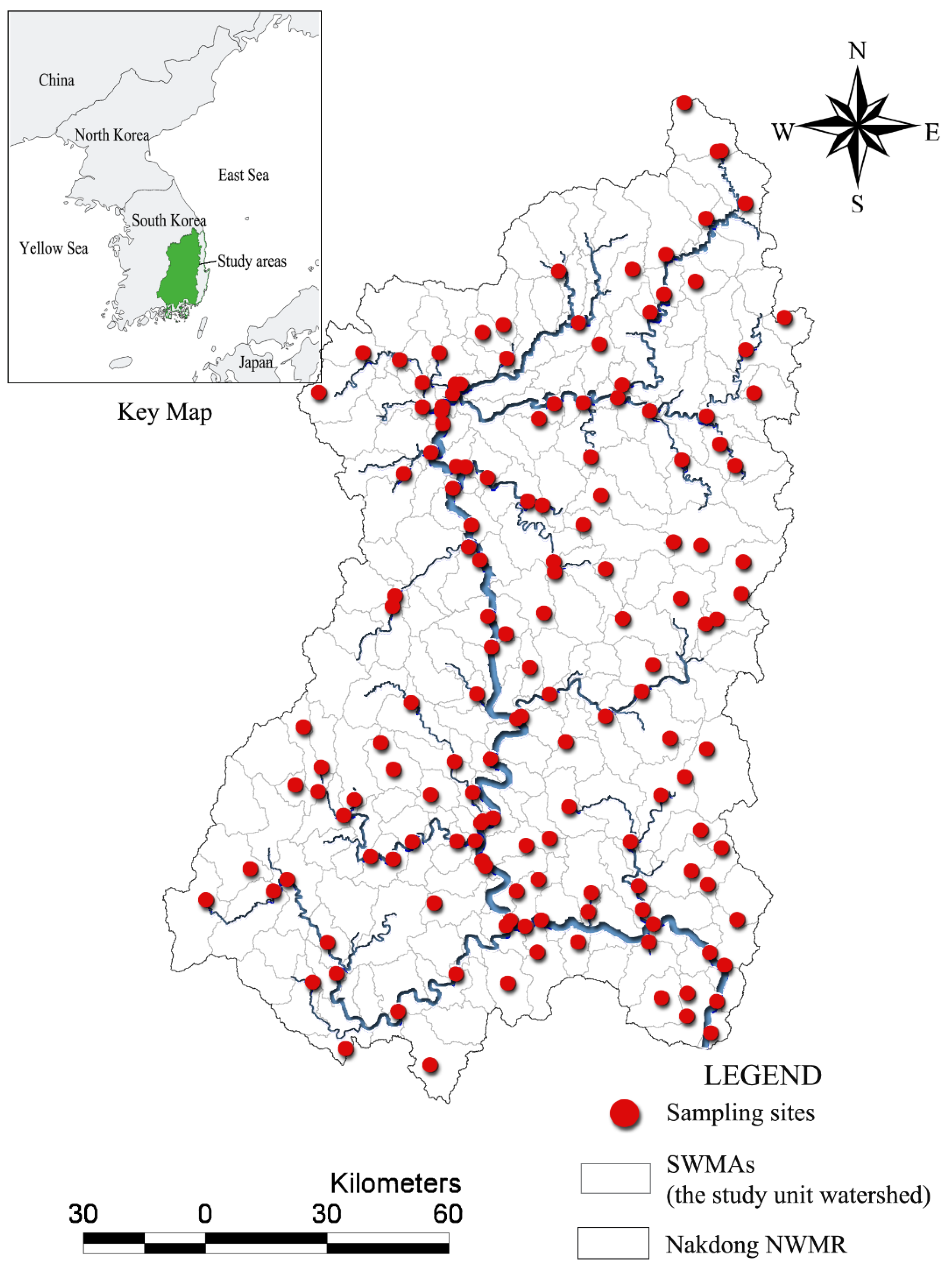
For the current study, we focused on a Nakdong national watershed management region (NWMR) containing 22 BWMRs and 191 SWMAs (Figure 1). We decided to use SWMAs as the study unit, because they are the basic unit of land use management for local governments and the MOE. Furthermore, we expected that the relationships between land use and biological indicators would be clearer at the SWMA level than at the NWMR or BWMR level.
The NAEMP has set up monitoring networks consisting of 1200 target sampling sites for the entire nation and 347 sites for the Nakdong river systems, including reference sites. Although not always the case, the target number of sampling sites under the monitoring program often corresponds approximately to the number of SWMAs. Owing to a limited budget, only 149 sites among the 347 target sites in the Nakdong river systems were monitored in 2011. As described earlier, we selected only 191 SWMAs belonging to the Nakdong river systems for our analysis. Some sampling sites in the study areas were not monitored in 2011, resulting in 148 sampling sites for the analysis (Figure 1).
The Nakdong River is the largest river within the Nakdong NWMR and the longest river system in Korea (525 km), covering most of the southeastern part of the Korean Peninsula. The majority of the streams in this watershed range from second to eighth order. According to the Korean Meteorological Administration, there has been no great change in precipitation over the last 30 years. The average annual precipitation for the last 30 years in the study areas was 1064 mm. However, the annual temperature has been gradually increasing from 12.9 °C in 1981 to 14.4 °C in 2010. The long-term annual average temperature for 1981–2010 was 14.1 °C, with the lowest average monthly temperature in January (−12.8 °C) and the highest in August (29.32 °C). Over the same period, average moisture and average wind speed were 61.6 (%), and 2.7 (m/s), respectively. The annual mean evapotranspiration was 1305.7 (mm). It is also noteworthy that approximately two-thirds of the total annual precipitation occurred during summer (June-September). Significant fluctuations in seasonal precipitation and water-flow levels are common in this area, and droughts often occur during winter and spring.

2.2. Biological Indicators and Water Quality

Using chemical parameters alone in stream management has been criticized as not fully capturing ecosystem dynamics [28,29]. For example, these parameters do not capture any information about the biological communities in streams [27]. Aquatic biota reflects the long-term cumulative effects of various anthropogenic disturbances [30] and are, therefore, crucial indicators of the ecosystem health of streams [28,31,32]. Various individual and aggregated indices for algae, macrophytes, macroinvertebrates, and fish have been proposed for the purposes of evaluating the ecological condition of streams and rivers [33,34,35,36,37,38]. Accordingly, the NAEMP has adopted and modified biological indicators for benthic diatoms, macroinvertebrates, and fish, as well as metrics for habitat quality based on indicators developed in other geographical areas (mainly North America and Europe). After reviewing a broad range of indices, the NAEMP adopted the TDI of Kelly and Whitton [39] for diatom communities, because it was developed based on the sensitivity and occurrence of a limiting nutrient (PO4-P) in freshwater systems. The sensitivity of the original TDI was evaluated using diatoms present in Korean rivers and streams, and the values for major taxa were amended accordingly. To evaluate macroinvertebrate communities, the NAEMP also adopted the KSI, which was constructed based on the method of Zelinka and Marvan [40]. Later, the KSI was modified and improved following the German standard method [41]. Since the introduction of the IBI by Karr [42], an IBI-type model using fish assemblages has been adopted by many countries. The 12 metrics originally proposed by Karr [42] were reduced to eight metrics after analysis of their properties according to the ecological characteristics of Korean fish assemblages in the NAEMP (for more detailed information on the biological indicators used by the NAEMP, see Lee et al. [27]). In the present study, we analyzed monitoring results from the NAEMP using TDI, KSI, and IBI in 2011, based on the mean values of spring and fall, ranging from 0 (very poor condition) to 100 (excellent condition) (Table 1). We adopted water quality parameters (biological oxygen demand (BOD), total nitrogen (T-N), total phosphorous (T-P), and chlorophyll-a (Chl-a)) as independent variables for biological indicators. We also measured mean elevation and slopes within a 1 km buffer of sampling sites.

2.3. Land Uses and Topographic Variables

To calculate the proportions of land use in watersheds at the SWMA level, we integrated the Land Use/Land Cover map released by the Ministry of Environment. The Land Use/Land Cover map of the Ministry of Environment was generated using the Landsat Thematic Mapper (30 m resolution) and Indian Remote Sensing-1C panchromatic (5.8 m resolution) images in 2007 and updated in 2011. The original Land Use/Land Cover map of the Ministry of Environment classified land use and land cover into 23 subcategories. For the current study, we reclassified the 23 subcategories into six categories: (a) developed areas including industrial, residential, roads, commercial, and bare soils; (b) agricultural areas; (c) paddy areas; (d) forested areas, including deciduous forest, coniferous forest, and mixed forest; (e) grassy areas including grassland and golf courses; and (f) wetlands. The area of each reclassified Land Use/Land Cover map category within each SWMA was computed in ArcMap and converted into proportional data for analysis. However, we included only two land use types for the study: forest and developed land. To compute topographic variables, including elevation and slope, we created a 1 km buffer from sampling sites, and computed the mean slope and elevation.

2.4. Geographically Weighted Regression (GWR) Model

OLS regression is the most common statistical tool used to explore the effects of independent variables (e.g., proportions of land use types) on a dependent variable (e.g., biological indicators). It is a global estimation technique that assumes spatial stationarity of the regression relationship and generates a single regression equation that best fits the variables for the entire study area. However, as discussed earlier, this global estimation technique does not capture local variations in the relationship between the proportions of different land uses and biological indicators. A typical OLS model for the relationship between land use and biological indicators might be:
y = β 0 +   i = 1 n β i x i +   ε
where y is the dependent variable (i.e., variance of biological indicators), β0 is the intercept, β1 is the coefficient of variable xi (i.e., proportion of land use type i), n is the number of independent variables (i.e., number of land use types), and ε is the error term. To estimate the local variation in proportions of land use with the above model, the locations of sampling sites need to be integrated into the equation as well:
y j =   β 0 ( u j +   v j ) +   i = 1 n β i ( u j +   v j ) x i +   ε
where uj and vj are the coordinates for each sampling location j, β0(uj+vj) is the intercept for sampling location j, and β1(uj+vj) is the local coefficient of proportion land use type i at location j [19,43,44,45,46,47,48]. From this perspective, the OLS model is a special case of the GWR model in which the parameter surface is assumed to be constant over space [20,44].
Equation (2) is a base GWR model for the biological indicators in this study. Rather than a single equation, it comprises an array of equations corresponding to different sampling sites. In GWR, an observation is weighted according to its proximity to sampling location j, with the result that the weighting of an observation is no longer constant in the calibration but varies with j. GWR is calibrated by weighting all observations around a sampling site using a distance decay function, which assumes that the observed values closer to the sampling location have higher impact on the local parameter estimates for the location [20,49]. The weighting function can be expressed in the exponential distance decay form as follows:
w j k =   e x p ( d j k 2   / h 2 )
where wjk is the weight of observation at sampling location k for the sampling location j, djk is the distance (meters, in this study) between sampling locations j and k, and h is referred to as the kernel bandwidth.
In GWR, there are two types of bandwidth options, fixed and adaptive. Fixed kernel bandwidth uses a constant bandwidth over study areas. In contrast, adaptive kernel bandwidth uses varying bandwidths based on data density: bandwidths are larger in locations where data are sparse and smaller where data are dense. In the current study, we used adaptive kernel bandwidth because of the inconsistent sampling densities over the study areas. The GWR model generated estimates the proportions for each land use type for each sampling site (i.e., local coefficient), the values of t-tests on the local parameter estimates, the local R2, and the local residuals. Non-stationary effects of land uses on biological indicators can, therefore, be visualized by mapping coefficients, t-statistics, and R2 values over the study areas.

2.5. Model Comparisons

The relative performance of the OLS and GWR models can be assessed by comparing R2 values, Akaike’s Information Criterion (AICc) [20], and spatial autocorrelation of residuals (Moran’s I). Greater R2 values indicate that variance in watershed land use explains a larger proportion of the variance in biological indicators in streams. Lower AICc values indicate a closer approximation of the model to the actual nature of the relationships between land uses and biological indicators [50].
Similar to conventional correlation coefficients, Moran’s I, a measure of spatial autocorrelation, ranges from −1 to 1. When the value of Moran’s I for the residuals of estimated models is close to zero, it suggests that the residuals are spatially independent. When the value is close to −1 or 1, it indicates that residuals are strongly spatially dependent [51]. We used the embedded software ArcToolbox in ArcMap to estimate GWR-derived and OLS-derived values for the TDI, KSI, and IBI indicators of benthic diatoms, macroinvertebrates, and fish, respectively, in the study areas. ArcMap GIS was also used to compute Moran’s I value and to visualize the non-stationarity of the effects of land uses in watersheds.

3. Results

3.1. Descriptive Statistics and Spatial Distributions

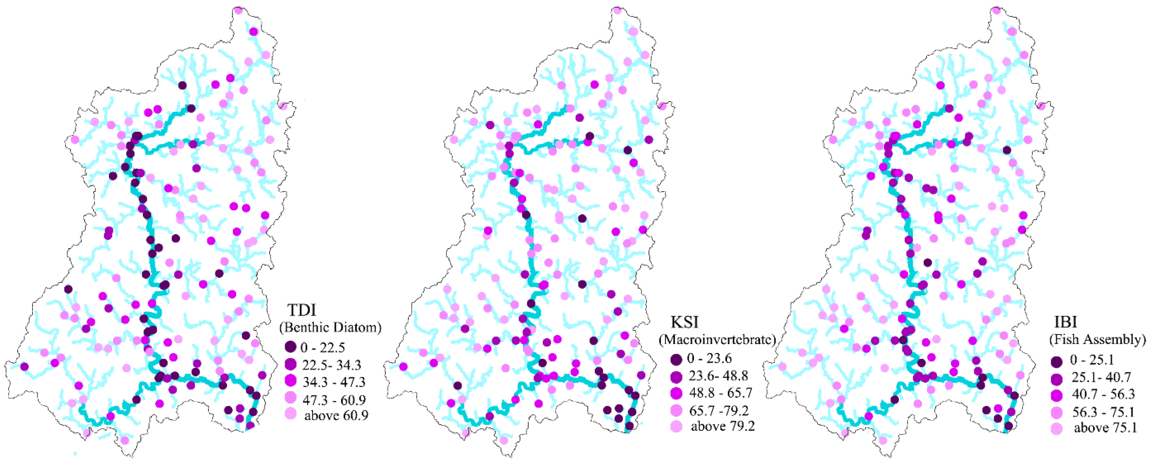
Ecological conditions measured by biological indicators, including TDI, KSI, and IBI, varied greatly among sampling sites (Table 2). Very low biological indicator values (near zero: very poor ecological condition) were observed at some sites, while others had very high values (near 100: very good ecological condition). The mean values of the TDI, KSI, and IBI within the study area were 43.27, 63.19, and 56.89, respectively. Overall, the condition of macroinvertebrate assemblies in the study areas was slightly better than the condition of benthic diatom or fish assemblies. The standard deviation of KSI values suggested greater variance in KSI values than in TDI or IBI values. Interestingly, all indicators reflected poor ecological conditions along main streams and in downstream areas in the southeastern part of the study region (Figure 2).
The mean values of the BOD, T-N, and T-P were 1.0, 2.24, and 0.04, respectively, indicating relatively good water quality in the areas investigated. However, the large standard deviation of elevation and slope indicate complex topographic characteristics in the study areas.
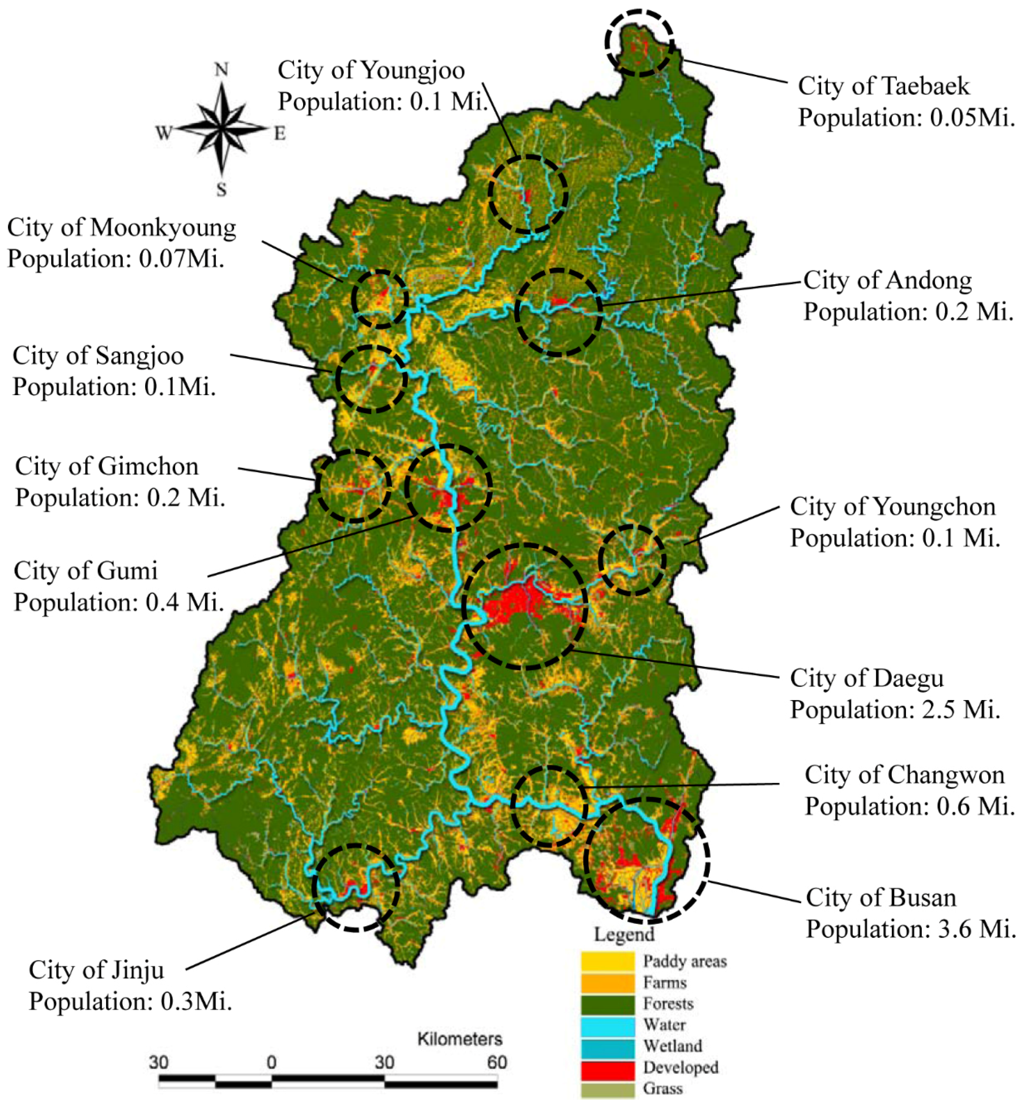
The relative proportions of each type of land use in watersheds also varied greatly across the study areas. The dominant land use type in the study area was forest (mean: 63.64%). Developed areas were relatively small, and concentrated at several sites along the main river, particularly near the central and downstream regions (Figure 3). As shown in Figure 3, several cities of various sizes were located near/along the main stream. Daegu and Busan were the two largest cities, with populations of 2.5 million and 3.5 million, respectively.
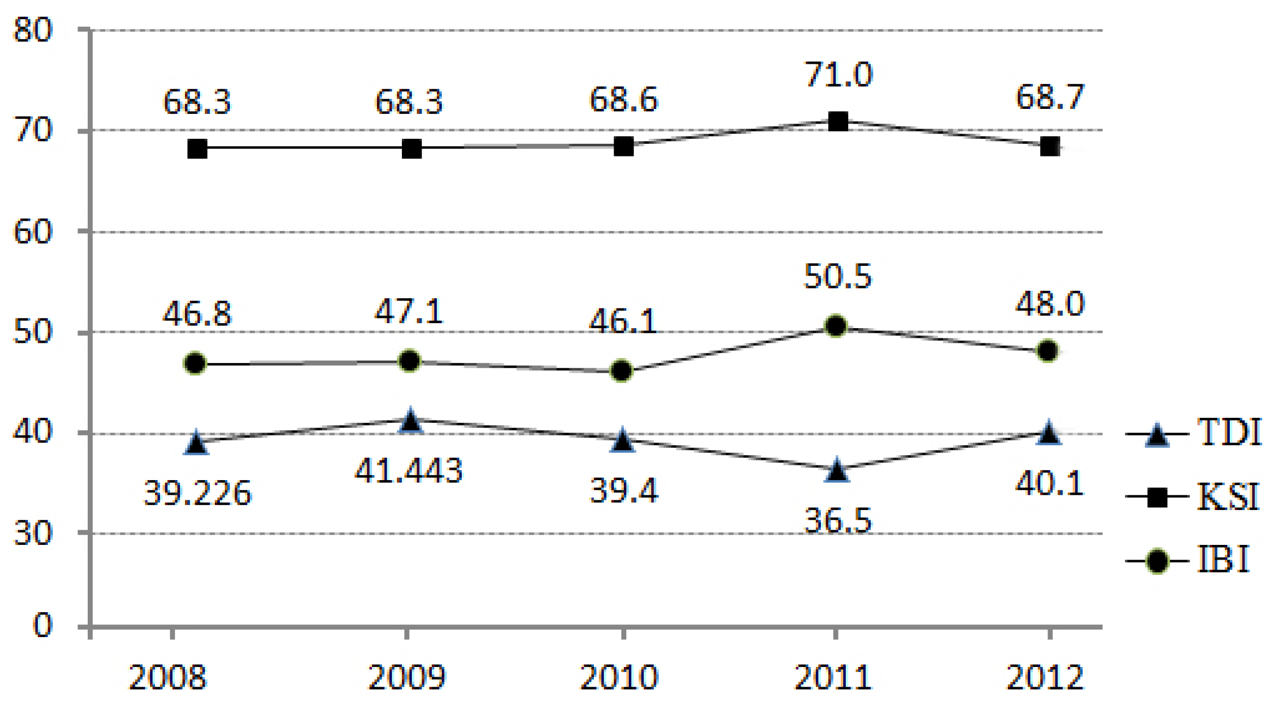
Before we undertook a detailed analysis, we considered the changes of the biological indicators over the five years from 2008 through to 2012 to understand the nature of the dataset (Figure 4). In 2011, there were changes in the biological indicators. KSI and IBI had slightly higher values, while TDI had slightly lower values, than the other years. Despite this fluctuation in the biological indicators in 2011, we used 2011 monitoring data to match with the most up-to-date land use/land cover data released by the Korean Ministry of Environment. Thus, there is a possibility that models estimated using datasets for other years might be slightly different from the model estimated using the 2011 dataset.

3.2. Selecting the Best Predictors for Biological Indicators

Before estimating the OLS and GWR models for each biological indicator, we conducted a preliminary regression analysis using the water quality parameters (i.e., BOD, T-N, T-P), topographic variables (i.e., elevation and slope), and land use parameters (i.e., developed areas, forested areas, agricultural areas, grass, wetland, and bare soils) to select the best predictive variables. To select the best-fit model for each biological indicator, we used the stepwise option in the SPSS for Windows software (SPSS Inc., Chicago, IL, USA) giving the R2, F-statistics, and t values (p < 0.05) of each variable.
In Table 3, a model with %forests, T-N, T-P, %bare soil, %wetland, and elevation had the highest adjusted-R2 (0.41) value for the TDI. For the KSI, a model with %developed areas and concentration of T-P had the highest R2 value (0.32, F = 22.50, p < 0.01). The percentage of forests, concentration of T-P, BOD, and elevation were the most significant variables for explaining the variance of IBI in the study region (adjusted-R2 = 0.42, F = 26.01, p < 0.01). From a land use perspective, the proportions of forests, developed areas, wetland, and grass in the watershed seemed to be significant variables for explaining the variances of the TDI, KSI, and IBI. In terms of water quality parameters, the concentration of T-P was the most significant determinant for all indicators, while the concentration of T-N and BOD was the most significant variable only for TDI and IBI, respectively.
In most previous studies dealing with the relationships between land use and water quality, the proportion of forest in the watersheds had a strong positive relationship with water quality parameters, while the percentage of developed areas had a strong negative relationship with water quality [1,2,3,4] and biological indicators [5,6,7,8,9,10,11,12]. However, it was rare for both variables to be significant in a regression model due to a negative mutual relationship. In our preliminary analysis, there was a strong negative correlation between %forest and %developed areas (r = 0.61) in the study areas. Despite there being other variables affecting the biological indicators, we focused on only two contrasting land use types (i.e., forest and developed areas) in our study. In particular, we investigated the spatial pattern of the coefficients of these two variables in GWR models for the TDI, KSI, and IBI when holding the other significant determinants constant.

3.3. Comparison between OLS and GWR Models

We compared the performance of the general OLS (global) and GWR (local) models for the TDI indicators (Table 4). In the global model, forest land had a positive effect (b = 0.25, β = 0.18) on TDI indicators, while the concentration of T-P and T-N had negative effects (b = −111.38, β = −0.32, b = −4.98, β = −0.21). Thus, a higher proportion of forest in watersheds may enhance the benthic diatom communities of streams. Conversely, a higher concentration of T-P and T-N had adverse effects on benthic diatom communities. The percentage of bare soil in the watershed appeared to have a negative impact on the TDI (b = −3.44, β = −0.24), while the percentage of wetland had a positive influence on the TDI (b = 5.27, β = 0.19). Elevation also had a positive effect on the TDI of streams (b = 0.02, β = 0.15). In the global model (OLS model), the intercept, land uses in watersheds (e.g., proportion of forest, bare soils, and wetland), water quality parameters (e.g., concentrations of T-N and T-P), and topographic characteristics (e.g., elevation) were significant at p < 0.01, and the global model was also significant overall (F = 16.71, p < 0.01).
The adjusted R2 of the global model was 0.41, indicating that 41% of the variance in the TDI across streams in the study area could be explained by three land use variables, two water quality parameters, and one topographic variable, while the remaining 59% was not explainable with these six variables. The R2 value of the GWR model was 0.44, which was slightly higher than the R2 value of the OLS model, suggesting that the GWR model performed better than the OLS model in explaining the variance of the TDI in the study areas. Similarly, the AICc values of the global and local models were 1165.43 and 1159.81, respectively. The lower AICc values of the GWR model also suggested a closer approximation of the model to the actual nature of the relationships between the dependent variables and TDI indicators. The Moran’s I value of the residuals in the local model was −0.10, which was slightly higher than in the global model (−0 09). However, the difference in the Moran’s I values for the two models was very small (0.01).
As discussed previously, the relative performance of the OLS and GWR models can be assessed based on the R2, AICc, and Moran’s I values of model residuals. Comparisons of these criteria suggested that the local model (GWR) performed better in explaining the variance of the TDI in the study areas and the presence of non-stationarity in the relationships between dependent variables, including the proportion of forest and TDI over space. The presence of non-stationarity suggested that the influence of forest on the TDI might vary over the study areas.
For the KSI, the proportion of the variation explained by the OLS model was modest (R2 = 0.33) (Table 5). About 32% of the KSI variance could be explained by the percentage of developed areas in the watershed (b = −2.87, β = −0.33), the concentration of T-P (b = −100.96, β = −0.25), and the percentage of grass areas (b = −4.77, β = −0.19), while the remaining 68% could not be explained by these variables. The high F- statistic (23.5, p < 0.01) for the OLS model suggests that this model was significant for the KSI. The results of this model further suggested an inverse relationship between the proportion of developed land in watersheds and the KSI values of streams. From a land use perspective, the proportion of developed land had the highest β value (−0.33) among the effective independent variables, including the concentration of T-P (β = −0.25) and proportion of grass areas (β = −0.19) in the OLS model.
The GWR model had the same R2 value (0.32) as the OLS model (0.32), suggesting that the GWR model explains almost the same amount of variance as the KSI. Furthermore, the similar AICc values of the OLS (1215.70) and GWR (1217.88) models revealed that both described the relationship between the independent variables and KSI to a similar degree of accuracy. The spatial autocorrelation indexes, measured by Moran’s I values, of the OLS (−0.04) and GWR (−0.06) models were very similar, suggesting that there was no significant spatial dependency of the residuals in the two models. The comparison between the two models of the KSI also indicated that non-stationarity effects were not present in the relationships between the KSI and independent variables, including the proportion of developed areas, the concentration of T-P, and the percentage of grass areas in watersheds.
For the IBI, the results of the global (OLS) model indicated that IBI values increased significantly with the proportion of forest within watersheds (b = 0.47, β = 0.32, p < 0.01) and elevated land (b = 0.03, β = 0.18, p < 0.01). Conversely, the IBI values were inversely related to the concentration of T-P (b = –81.91, β = −0.23, p < 0.01) and BOD (b = −5.99, β = −0.22, p < 0.01). The adjusted R2 of the global model was 0.42, indicating that ~42% of the variance in the IBI among streams can be explained by the four variables of forests, T-P, BOD, and elevation. The F-value (26.57) of the OLS model was significant (p < 0.01) (Table 6).
The R2 value of the GWR model (0.49) was considerably higher than that of the OLS, and suggested that ~49% of the variance in the IBI among study sites could be explained by the proportions of forests, T-P, BOD, and elevation. The GWR model also had a lower AIC value (1165.13) than that of the OLS model (1171.27). Both the higher R2 value and the lower AIC value strongly indicate that the GWR model performed better in terms of explaining the IBI variance and approximating reality. Furthermore, the lower Moran’s I value (–0.01) of the GWR model compared with the OLS model (0.07) indicates that the residuals in the former model exhibited less spatial dependency. The higher R2, lower AICc and lower Moran’s I of the GWR model strongly suggest the presence of non-stationarity between the independent variables and IBI in the study areas. The presence of non-stationarity in the relationships suggests that the influence of the proportion of forest, along with other independent variables, might vary stream by stream in the study areas.
Overall, the results of the OLS models (Table 4, Table 5 and Table 6) indicated that the selected variables for each biological indicator could explain ~41%, 32%, and 42% of the variance in the TDI, KSI, and IBI, respectively. No considerable differences between the OLS and GWR models were observed for the KSI indicators. The estimated OLS and GWR models of the KSI had almost the same R2, AICc, and Moran’s I values suggesting that there might be no non-stationary effects of land use, water quality, and topographic variables for the KSI models. Compared to the OLS model, the considerably higher R2 value and β-value of the GWR model for the TDI and IBI indicated that, according to this model, the TDI and IBI were more sensitive to the heterogeneity of forest coverage than the KSI. Therefore, a higher percentage of forest land in watersheds may substantially enhance the ecological conditions as measured by the RDI and IBI, and the relationships between forests and two indicators (i.e., TDI and IBI) might vary over space (i.e., non-stationary effects). Interestingly, the negative impacts of developed areas were found only in the OLS model for the KSI implying that the higher proportion of developed areas in watersheds can adversely affect the KSI to a greater extent than the other biological indicators.
Positive influences of forests were found in the TDI and IBI models, suggesting that a higher proportion of forests in watersheds may enhance the TDI and IBI in streams. Interestingly, land use (developed areas or forests) in watersheds appeared to be a more significant variable than water quality parameters or topographic variables in the KSI and IBI models. In the TDI model, a water quality parameter (i.e., T-P) was more significant than land use or topographic variables.
In contrast to the OLS model, the GWR model assumes non-stationarity in the relationship between a dependent variable (i.e., a biological indicator) and independent variable (i.e., the proportions of forest or developed land in watersheds). In the comparison of the performance of the OLS and GWR models, the GWR models of the KSI were not able to better explain the variances of the KSI in the study areas. However, the GWR model of the TDI and IBI clearly performed better than the OLS model in terms of the R2, AICc, and spatial autocorrelation index values (i.e., Moran’s I). The GWR model is based on non-stationary effects (Equation (2)), while the OLS model is based on stationary effects (Equation (1)). Therefore, the superior performance of the GWR models strongly suggests non-stationarity in the effects of land use (i.e., forests) on biological indicators (i.e., the TDI and IBI). The OLS model might be an effective tool for understanding regionally averaged effects of land use on ecological conditions, but this global model cannot capture local variations in such effects. For some watersheds and indicator types, the OLS model might overestimate or underestimate the effects of land use.

3.4. Description of Local Estimated Land Use Effects in GWR models

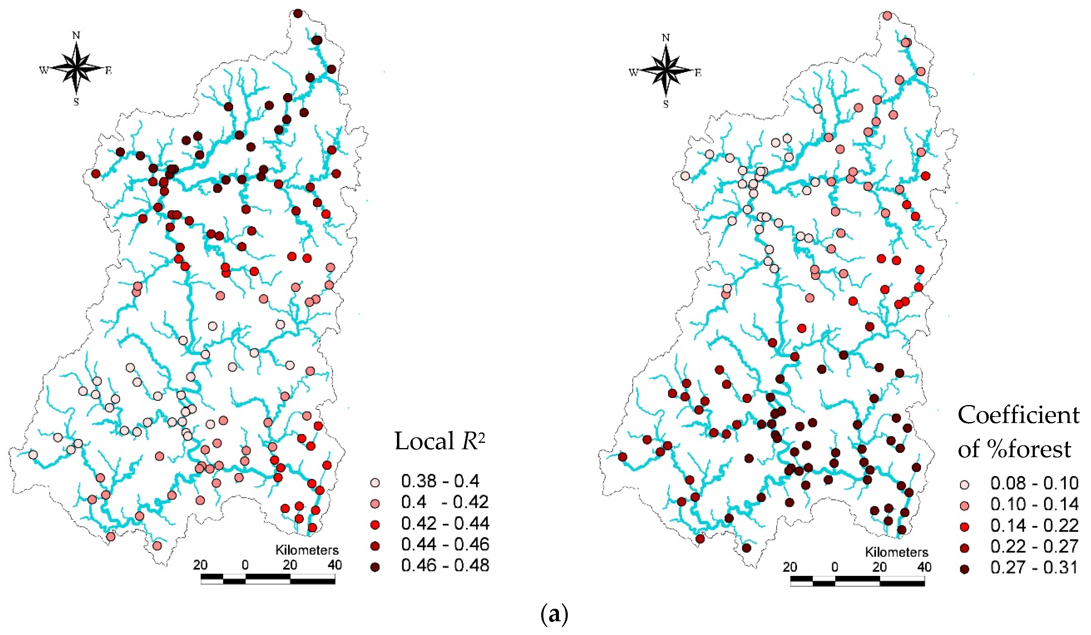
In the GWR models, descriptive statistics for local R2 and land use coefficients for the TDI, KSI, and IBI vary greatly in each GWR model (Table 7). For example, the proportion of forest with other variables in the local (GWR) TDI model could explain about 38% (minimum) of the variance in the TDI among streams in some watersheds, while it could explain 48% (maximum) of the variance in the TDI among other streams. Similarly, the coefficients of the proportions of forest varied to a considerable degree among watersheds, ranging from 0.08 to 0.31. Despite this variation, TDI values always increased with the proportion of forest land. The mean R2 and coefficient values for forests in the local TDI model were 0.44 and 0. 20, respectively.
Similarly, we also found a large degree of variance in R2 values and the coefficients of developed land in the local KSI model. In particular, the changes of R2 values in the KSI models surprisingly varied watershed by watershed. In some watersheds, the proportion of developed areas and other variables explained a small proportion of the KSI variance (15%), while in other areas they explained up to 41% of the variance. The proportion of developed areas in watersheds had a negative relationship with the KSI, ranging from −3.12 to −2.31.
The R2 of the GWR model for the IBI also varied considerably among the study areas, ranging from 0.27 to 0.54. This variance indicates that the proportion of forests, T-P, BOD, and elevation were not consistently able to explain IBI values over space. Although the effect varied significantly (−0.03 –0.98), higher proportions of forest in watersheds were associated with increased IBI values in streams. The mean value for the coefficient of the proportion of forest areas was 0.39, the minimum value was −0.03, and the maximum value was 0.98. It is interesting to note that, while in most watersheds the proportion of forests was associated with increased IBI values for streams, in some watersheds forests had a negligible (or even negative) relationship with IBI values (Table 7). The standard deviation of %developed (SD = 0.25) land in the KSI local model and %forest (SD = 0.30) in the IBI local model were relatively high.
Scatterplots between observed and predicted values of the TDI local model indicate that most sites fell within the 95% confidence range of the estimated GWR model. It seemed that the observed values in the low range of TDI values were underestimated in the GWR model (Figure 5a). The KSI-GWR model showed a clear relationship in the middle–high range of KSI values. The GWR model overestimated in the range of observed KSI values from 20 to 40, while it underestimated in the range from 0 to 20. Seven watersheds were outside the 95% confidence interval (Figure 5b). The IBI-GWR model produced an even more complex estimation pattern. In the high range, three watersheds were overestimated, and one watershed was underestimated. In the middle range, one was overestimated and one was underestimated. In the low range of IBI values, two watersheds were underestimated in the GWR model (Figure 5c).

3.5. Spatial Distribution of the Estimated Parameters of GWR models

GIS mapping technology is an effective means of visualizing the variability of local R2 and land use coefficients in local GWR models for the TDI, KSI, and IBI indicators (Figure 6). Within the study region, higher R2 values (dark red dots) of the GWR model for the TDI indicator (Figure 6a) were observed mostly in the upstream areas, while lower R2 values (cream color) were located mainly in the middle stream areas. In these regions, the forests and other variables explained a relatively small proportion of the TDI variability. Higher forest coefficient values (dark red) were concentrated in downstream areas, suggesting a relatively higher influence of forests on the TDI in these areas. In contrast, lower coefficients for forest in the estimated GWR model were observed mostly in middle-stream areas, while the upstream areas produced mid-range coefficients for forests (red dots). Despite the spatial variation, TDI values were always increased by forests (Figure 6a).
Higher R2 values in estimated GWR models for TDI and IBI were observed in upstream areas, where forests were relatively well preserved and land development was less extensive. Conversely, the higher R2 values in the estimated GWR model for the KSI were concentrated in downstream areas. Interestingly, both the proportion of forest and developed areas had relatively higher coefficient values in downstream areas in the estimated GWR models for the TDI, KSI, and IBI.

4. Discussion

Forests and developed land have contrasting effects on stream biological communities (e.g., diatoms, macroinvertebrates, and fish) in watersheds. Previous studies have shown that greater proportions of forest coverage are consistently associated with a more favorable ecological status for streams [5,6,7,52,53,54,55,56,57]. In contrast, greater proportions of developed land in watersheds are consistently associated with significantly poorer ecological conditions, as measured by various biological indicators [6,7,52,53,56,58,59,60,61]. Adverse effects of agricultural land use in watersheds on biological indicators are also well documented [7,11,62,63].
Our OLS models for the TDI, KSI, and IBI indicators confirmed previous research reporting negative effects of developed land (e.g., urbanized or impervious areas) and positive effects of forest on biological indicators in watersheds. Forests had positive impacts on the TDI and IBI, while developed areas had a negative influence on the KSI.
Most previous studies focusing on the relationship between land use in watersheds and the ecological conditions of streams have adopted conventional correlation or regression methods, which are unable to capture spatial variability among study sites. However, land development in watersheds alters not only the watershed itself, but also various environmental conditions in adjacent streams (e.g., water temperature, stream channel morphology, and the dynamics of sediments and water). Land development also affects hydrologic regimes and increases pollutant loads. These factors may have independent or interacting impacts on aquatic organisms [64]. Furthermore, different regions vary greatly in their topography (e.g., elevation, slope, soil type, etc.), watershed characteristics (e.g., size, composition, and distance from main cities), and stream environments (e.g., stream order, type and width; channel type; sediments; riparian areas). Therefore, it is unreasonable to assume that all landscapes, watersheds, and streams are affected in the same way and to the same degree by the presence of developed land or forests.
Our GWR models for the TDI and IBI strongly suggested a non-stationarity in the influence of forest in the watershed. Significant differences between the OLS and GWR models for the TDI and IBI in terms of R2, AIC, and Moran’s I values (Table 4 and Table 6) suggested a better performance of the GWR models for explaining the variance of TDI and IBI in streams. This provides strong evidence that the effects of forests on the TDI and IBI indicators were non-stationary. Magner et al. (2008) [62] reported similar results, indicating that land use effects on biological parameters in streams could vary by location due to the localized geology. In their study on grazed riparian management and stream channel responses in Southeastern Minnesota streams, they found that land use metrics had no significant relationship with ordination axes, and they explained that the localized geology associated with producing stream bed cobbles has a stronger influence on the site than the land uses in the watershed.
However, as pointed out by Brunsdon et al. [43,44], it is difficult to measure the underlying mechanisms of spatial variability in the effects of land. Potential contributors to this spatial variability include differences in watershed characteristics, pollution sources, and degrees of urbanization [4,13]. In addition, variables such as topography, stream environments, and precipitation levels may also play a role in spatial variability. We tried to include available water quality variables (i.e., BOD, T-N, and T-P) and topographic variables (elevation and slope) when estimating the OLS and GWR models.
However, the reason for using these models was not to investigate the underlying mechanisms of the variables used in estimating the models. The OLS model was used to determine the overall influence of land uses in water environments (i.e., water quality parameters and topographic variables) on biological indicators, regardless of the location of sampling sites, while the GWR was used to investigate the spatial variation of land uses on biological indicators. To understand the mechanism of land use effects on biological indicators, the use of a structural equation modeling (SEM) [65] and path analysis [66] should be considered. Nevertheless, our GWR models clarify our understanding of the localized responses of stream organisms to land use. Given the complexity of this system, it is beyond the scope of the present study to measure all of the factors affecting the spatial variability of the effects of land use and the underlying mechanism of the pathways that influence them.

5. Conclusions

Many previous studies investigating the relationship between land use and the ecological response of stream biota have used correlation and regression analyses (OLS), which assume stationarity of the effects. However, in the present study, we found that the relationship between land use and stream ecology was spatially variable (i.e., non-stationary). We used OLS models (global) and GWR models (local) to analyze the effects of contrasting land uses (forest and developed land) on the TDI, KSI, and IBI indicators, representing the ecological status of benthic diatom, macroinvertebrate, and fish assemblages, respectively. The performances of these two types of models were then compared based on R2, AIC, and Moran’s I values. Compared with the OLS models of the TDI and IBI, the GWR models of the TDI and IBI were better able to reveal details of the effects of particular land use types in specific locations; however, OLS models may be more useful in other applications. For example, OLS models may provide an effective means of assessing general trends within larger regions. Furthermore, OLS models may be more practical for creating environmental policies, while GWR may be more useful for effectively applying such policies to specific target streams or watersheds.
The effects of land use in watersheds can also vary among stream organisms. R2 and land use coefficients varied considerably among GWR models for different biological indicators, suggesting that different biological assemblages respond to different land uses in different ways. Differences in the sensitivities of biological assemblages to land use may help explain the observed variations in R2 and land use coefficients.
Although the present study demonstrates the utility of GWR models for understanding location-specific relationships between land use and stream communities, some critical questions remain to be answered. In particular, it will be important to investigate the underlying mechanisms of the impact of forest and developed land on stream biota, as well as for the spatial variability in these effects. We discuss several potential explanatory factors above; however, these will be challenging to study if they vary significantly among study sites. Further studies are, therefore, needed to elucidate more fully the effects of land use on stream biological communities, the reasons for their spatial variation, and the associated principles that can be derived, to manage the ecological integrity of streams more intelligently and effectively. It may also be possible to use regression tree analysis [67], SEM [65], path analysis [66], and non-metric multidimensional scaling [68,69] to explore the underlying mechanism of land use effects on biological indicators in streams, avoiding spatial autocorrelation issues, and to support decision-makers in watershed-specific land use management in minimizing the adverse impacts of land use on ecological communities of streams.

Acknowledgments

This study was conducted under the project “National Aquatic Ecosystem Health Survey and Assessment” in Korea, and was supported by the Ministry of the Environment and the National Institute of Environmental Research, Korea.

Author Contributions

All of the authors contributed extensively to the work. Kyoung-Jin An and Sang-Woo Lee designed the research, performed the data analysis, and wrote the manuscript. Soon-Jin Hwang, Se-Rin Park, and Sun-Ah Hwang contributed to the data interpretation, discussion, and editing of the manuscript.

Conflicts of Interest

The authors declare no conflict of interest.

References

  1. Sliva, L.; Williams, D.D. Buffer zone versus whole catchment approaches to studying land use impact on river water quality. Water Res. 2001, 35, 3462–3472. [Google Scholar] [CrossRef]
  2. Tong, S.T.Y.; Chen, W. Modeling the relationship between land use and surface water quality. J. Environ. Manag. 2002, 66, 377–393. [Google Scholar] [CrossRef]
  3. Mehaffey, M.H.; Nash, M.S.; Wade, T.G.; Ebert, D.W.; Jones, K.B.; Rager, A. Linking land cover and water quality in New York City’s water supply watersheds. Environ. Monit. Assess. 2005, 107, 29–44. [Google Scholar] [CrossRef] [PubMed]
  4. Tu, J.; Xia, Z.G. Examining spatially varying relationships between land use and water quality using geographically weighted regression I: Model design and evaluation. Sci. Total Environ. 2008, 407, 358–378. [Google Scholar] [CrossRef] [PubMed]
  5. Weaver, L.A.; Garman, G.C. Urbanization of a watershed and historical changes in a stream fish assemblage. Trans. Am. Fish. Soc. 1994, 123, 162–172. [Google Scholar] [CrossRef]
  6. Wang, L.; Lyons, J.; Kanehl, P.; Gatti, R. Influences of watershed land use on habitat quality and biotic integrity in Wisconsin streams. Fisheries 1997, 22, 6–12. [Google Scholar] [CrossRef]
  7. Moore, A.A.; Palmer, M.A. Invertebrate biodiversity in agricultural and urban headwater streams: Implications for conservation and management. Ecol. Appl. 2005, 15, 1169–1177. [Google Scholar] [CrossRef]
  8. Steffy, L.Y.; Kilham, S.S. Effects of urbanization and land use on fish communities in Valley Creek watershed, Chester County, Pennsylvania. Urban Ecosyst. 2006, 9, 119–133. [Google Scholar] [CrossRef]
  9. Meador, M.R.; Coles, J.F.; Zappia, H. Fish assemblage responses to urban intensity gradients in contrasting metropolitan areas: Birmingham, Alabama, and Boston, Massachusetts. In Effects of Urbanization on Stream Ecosystems; Brown, L.R., Gray, R.H., Hughes, R.M., Meador, M.R., Eds.; American Fisheries Society: Bethesda, MD, USA, 2005; pp. 409–422. [Google Scholar]
  10. Lee, S.W.; Hwang, S.J.; Lee, S.B.; Hwang, H.S.; Sung, H.C. Landscape ecological approach to the relationships of land use patterns in watersheds to water quality characteristics. Landsc. Urban Plan. 2009, 92, 80–89. [Google Scholar] [CrossRef]
  11. Park, S.R.; Lee, H.J.; Lee, S.W.; Hwang, S.J.; Byeon, M.S.; Joo, G.J.; Jeong, K.S.; Kong, D.S.; Kim, M.C. Relationships between land use and multi-dimensional characteristics of streams and rivers at two different scales. Ann. Limnol. Int. J. Limnol. 2011, 47, S107–S116. [Google Scholar] [CrossRef]
  12. Utz, R.M.; Hilderbrand, R.H.; Raesly, R.L. Regional differences in patterns of fish species loss with changing land use. Biol. Conserv. 2010, 143, 688–699. [Google Scholar] [CrossRef]
  13. Tu, J. Spatially varying relationships between land use and water quality across an urbanization gradient explored by geographically weighted regression. Appl. Geogr. 2011, 31, 376–392. [Google Scholar] [CrossRef]
  14. Casetti, E. Generating models by the expansion method: Applications to geographical research. Geogr. Anal. 1972, 4, 81–91. [Google Scholar] [CrossRef]
  15. Jones, J.; Casetti, E. Applications of the Expansion Method; Routledge: London, UK, 1992. [Google Scholar]
  16. Foster, S.A.; Gorr, W.L. An adaptive filter for estimating spatially-varying parameters: Application to modeling police hours spent in response to calls for service. Manag. Sci. 1986, 32, 878–889. [Google Scholar] [CrossRef]
  17. Gorr, W.L.; Olligschlaeger, A.M. Weighted spatial adaptive filtering: Monte Carlo studies and application to illicit drug market modeling. Geogr. Anal. 1994, 26, 67–87. [Google Scholar] [CrossRef]
  18. Goldstein, H. Multilevel Models in Educational and Social Research; Oxford University Press: London, UK, 1987. [Google Scholar]
  19. Brunsdon, C.; Fotheringham, A.S.; Charlton, M.E. Geographically Weighted Regression: A Method for Exploring Spatial Nonstationarity. Geogr. Anal. 1996, 28, 281–298. [Google Scholar] [CrossRef]
  20. Fotheringham, A.S.; Brunsdon, C.; Charlton, M.E. Geographically Weighted Regression: The Analysis of Spatially Varying Relationships; Wiley: Chichester, UK, 2002. [Google Scholar]
  21. Propastin, P. Modifying geographically weighted regression for estimating aboveground biomass in tropical rainforests by multispectral remote sensing data. Int. J. Appl. Earth Obs. Geoinf. 2012, 18, 82–90. [Google Scholar] [CrossRef]
  22. Lu, B.; Charlton, M.; Fortheringham, A.S. Geographically weighted regression using a non-euclidean distance metric with a study on London house price data. Procedia Environ. Sci. 2011, 7, 92–97. [Google Scholar] [CrossRef]
  23. Saphores, J.D.; Li, W. Estimating the value of urban green areas: A hedonic pricing analysis of the single family housing market in Los Angeles, CA. Landsc. Urban Plan. 2012, 104, 373–387. [Google Scholar] [CrossRef]
  24. Kamarianakis, Y.; Feidas, H.; Kokolatos, G.; Chrysoulakis, N.; Karatzias, V. Evaluating remotely sensed rainfall estimates using nonlinear mixed models and geographically weighted regression. Environ. Model. Softw. 2008, 23, 1438–1447. [Google Scholar] [CrossRef]
  25. Szymanowski, M.; Kryza, M. Application of geographically weighted regression for modelling the spatial structure of urban heat island in the city of Wroclaw (SW Poland). Procedia Environ. Sci. 2011, 3, 87–92. [Google Scholar] [CrossRef]
  26. Moran, P.A.P. Notes on Continuous Stochastic Phenomena. Biometrika 1950, 37, 17–23. [Google Scholar] [CrossRef] [PubMed]
  27. Lee, S.W.; Hwang, S.J.; Lee, J.K.; Jung, D.I.; Park, Y.J.; Kim, J.T. Overview and application of the National Aquatic Ecological Monitoring Program (NAEMP) in Korea. Ann. Limnol. Int. J. Limnol. 2011, 47, S3–S14. [Google Scholar] [CrossRef]
  28. Davis, W.S.; Simon, T.P. Biological Assessment and Criteria: Tools for Water Resource Planning and Decision Making; CRC Press: New York, NY, USA, 1995. [Google Scholar]
  29. McCarron, E.; Frydenborg, R. The Florida bioassessment program: An agent of change. Hum. Ecol. Risk Assess. Int. J. 1997, 3, 967–977. [Google Scholar] [CrossRef]
  30. Karr, J.R.; Chu, E.W. Restoring Life in Running Waters: Better Biological Monitoring; Island Press: Washington, DC, USA, 1999. [Google Scholar]
  31. US EPA. Summary of Biological Assessment Programs and Biocriteria Development for States, Tribes, Territories, and Interstate Commissions: Streams and Wadeable Rivers (EPA-822-R-02-048); U.S. Environmental Protection Agency, Office of Water Regulations and Standards: Washington, DC, USA, 2002.
  32. Simon, T.P. Assessing the Sustainability and Biological Integrity of Water Resources Using Fish Communities; CRC Press: New York, NY, USA, 1999; p. 652. [Google Scholar]
  33. Osborne, P.E.; Suárez-Seoane, S. Should data be partitioned spatially before building large-scale distribution models? Ecol. Model. 2002, 157, 249–259. [Google Scholar] [CrossRef]
  34. Hering, D.; Johnson, R.K.; Kramm, S.; Schmutz, S.; Szoszkiewicz, K.; Verdonschot, P.F.M. Assessment of European streams with diatoms, macrophytes, macroinvertebrates and fish: A comparative metric-based analysis of organism response to stress. Freshw. Biol. 2006, 51, 1757–1785. [Google Scholar] [CrossRef]
  35. Pont, D.; Hugueny, B.; Beier, U.; Goffaux, D.; Melcher, A.; Noble, R.; Rogers, C.; Roset, N.; Schmutz, S. Assessing river biotic condition at a continental scale: A European approach using functional metrics and fish assemblages. J. Appl. Ecol. 2006, 43, 70–80. [Google Scholar] [CrossRef]
  36. Johnson, R.K.; Furse, M.T.; Hering, D.; Sandin, L. Ecological relationships between stream communities and spatial scale: Implications for designing catchment-level monitoring programmes. Freshw. Biol. 2007, 52, 939–958. [Google Scholar] [CrossRef]
  37. Ode, P.; Hawkins, C.; Mazor, R. Comparability of biological assessments derived from predictive models and multimetric indices of increasing geographic scope. J. North Am. Benthol. Soc. 2008, 27, 967–985. [Google Scholar] [CrossRef]
  38. Stoddard, J.L.; Herlihy, A.T.; Peck, D.V.; Hughes, R.M.; Whittier, T.R.; Tarquinio, E. A process for creating multimetric indices for large-scale aquatic surveys. J. North Am. Benthol. Soc. 2008, 27, 878–891. [Google Scholar] [CrossRef]
  39. Kelly, M.G.; Whitton, B.A. The trophic diatom index: A new index for monitoring eutrophication in rivers. J. Appl. Phycol. 1995, 7, 433–444. [Google Scholar] [CrossRef]
  40. Zelinka, M.; Marvan, P. Zur präzisierung der biologischen klassifikation der reinheit fließender gewässer. Arch. Hydrobiol. 1961, 57, 389–407. [Google Scholar]
  41. DIN, Biological-Ecological Analysis of Water (Group M): Determination of the Saprobic Index (M2). German Standard Methods for the Examination for Water, Wastewater and Sludge; DIN 38410, Part 2; Beuth Verlag GmbH: Berlin, Germany, 1990; p. 10.
  42. Karr, J.R. Assessment of biological integrity using fish communities. Fisheries 1981, 6, 21–27. [Google Scholar] [CrossRef]
  43. Brunsdon, C.; Fotheringham, S.; Charlton, M. Geographically Weighted Regression-modelling spatial non-stationarity. J. R. Stat. Soc. Ser. D Stat. 1998, 47, 431–443. [Google Scholar] [CrossRef]
  44. Brunsdon, C.; Fotheringham, A.S.; Charlton, M. Spatial nonstationarity and autoregressive models. Environ. Plan. A 1998, 30, 957–973. [Google Scholar] [CrossRef]
  45. Fotheringham, A.S.; Charlton, M.; Brunsdon, C. The geography of parameter space: An investigation of spatial non-stationarity. Int. J. Geogr. Inf. Syst. 1996, 10, 605–627. [Google Scholar] [CrossRef]
  46. Fotheringham, A.S. Trends in quantitative methods I: Stressing the local. Prog. Hum. Geogr. 1997, 21, 88–96. [Google Scholar] [CrossRef]
  47. Fotheringham, A.S.; Charlton, M.E.; Brunsdon, C. Two techniques for exploring non-stationarity in geographical data. Geogr. Syst. 1997, 4, 59–82. [Google Scholar]
  48. Fotheringham, A.S.; Charlton, M.E.; Brunsdon, C. Geographically Weighted Regression: A Natural Evolution of the Expansion Method for Spatial Data Analysis. Environ. Plan. A 1998, 30, 1905–1927. [Google Scholar] [CrossRef]
  49. Fotheringham, A.S. Quantification, evidence and positivism. In Approaches to Human Geography; Valentine, G., Aitken, S., Eds.; Sage: London, UK, 2006. [Google Scholar]
  50. Wang, Q.; Ni, J.; Tenhunen, J. Application of a geographically-weighted regression analysis to estimate net primary production of Chinese forest ecosystems. Glob. Ecol. Biogeogr. 2005, 14, 379–393. [Google Scholar] [CrossRef]
  51. Fortin, M.J.; Drapeau, P.; Legendre, P. Spatial autocorrelation and sampling design in plant ecology. Vegetatio 1989, 83, 209–222. [Google Scholar] [CrossRef]
  52. Lenat, D.R.; Crawford, J.K. Effects of land use on water quality and aquatic biota of three North Carolina Piedmont streams. Hydrobiologia 1994, 294, 185–199. [Google Scholar] [CrossRef]
  53. Wallace, J.B.; Eggert, S.L.; Meyer, J.L.; Webster, J.R. Multiple trophic levels of a forest stream linked to terrestrial litter inputs. Science 1997, 277, 102–104. [Google Scholar] [CrossRef]
  54. Welsh, H.H.; Lind, A.J. Multiscale habitat relationships of stream amphibians in the Klamath-Siskiyou Region of California and Oregon. J. Wildl. Manag. 2002, 66, 581–602. [Google Scholar] [CrossRef]
  55. Wipfli, M.S.; Gregovich, D.P. Export of invertebrates and detritus from fishless headwater streams in southeastern Alaska: Implications for downstream salmonid production. Freshw. Biol. 2002, 47, 957–969. [Google Scholar] [CrossRef]
  56. Allan, J.D. Landscapes and riverscapes: The influence of land use on stream ecosystems. Annu. Rev. Ecol. Evol. Syst. 2004, 35, 257–284. [Google Scholar] [CrossRef]
  57. Olson, D.H.; Weaver, G. Vertebrate assemblages associated with headwater hydrology in western Oregon managed forests. For. Sci. 2007, 53, 343–355. [Google Scholar]
  58. Yoder, C.O.; Miltner, R.; White, D. Using biological criteria to assess and classify urban streams and develop improved landscape indicators. In National Conference on Tools for Urban Water Resource Management and Protection; U.S. Environmental Protection Agency: Washington, DC, USA, 2000. [Google Scholar]
  59. Roy, A.H.; Rosemond, A.D.; Paul, M.J.; Leigh, D.S.; Wallace, J.B. Stream macroinvertebrate response to catchment urbanisation (Georgia, USA.). Freshw. Biol. 2003, 48, 329–346. [Google Scholar] [CrossRef]
  60. Morse, C.C.; Huryn, A.D.; Cronan, C. Impervious surface area as a predictor of the effects of urbanization on stream insect communities in Maine, USA. Environ. Monit. Assess. 2003, 89, 95–127. [Google Scholar] [CrossRef] [PubMed]
  61. Miltner, R.J.; White, D.; Yoder, C. The biotic integrity of streams in urban and suburbanizing landscapes. Landsc. Urban Plan. 2004, 69, 87–100. [Google Scholar] [CrossRef]
  62. Magner, J.A.; Vondracek, B.; Brooks, K.N. Grazed riparian management and stream channel response in Southeastern Minnesota (USA) streams. Environ. Manag. 2008, 42, 377–390. [Google Scholar] [CrossRef] [PubMed]
  63. Omernik, J.M.; Abernathy, A.R.; Male, L.M. Stream nutrient levels and proximity of agricultural and forest land to streams: Some relationships. J. Soil Water Conserv. 1981, 36, 227–231. [Google Scholar]
  64. Walsh, C.J.; Roy, A.H.; Feminella, J.W.; Cottingham, P.D.; Groffman, P.M.; Morgan, R.P. The urban stream syndrome: Current knowledge and the search for a cure. J. North Am. Benthol. Soc. 2005, 24, 706–723. [Google Scholar] [CrossRef]
  65. Rabe-Hesketh, S.; Skrondal, A.; Pickles, A. Generalized multilevel structural equation modeling. Psychometrika 2004, 69, 167–190. [Google Scholar] [CrossRef]
  66. Streiner, D.L. Finding Our Way: An Introduction to Path Analysis. Can. J. Psychiatry 2005, 50, 115–122. [Google Scholar] [PubMed]
  67. Breiman, L.; Friedman, J.H.; Olshen, R.A.; Stone, C.J. Classification and Regression Trees, 2nd ed.; Pacific Grove: Wadsworth, CA, USA, 1984. [Google Scholar]
  68. Kruskal, J.B. Multidimensional scaling by optimizing goodness of fit to a nonmetric hypothesis. Psychometrika 1964, 29, 1–27. [Google Scholar] [CrossRef]
  69. Mather, P.M. Computational Methods of Multivariate Analysis in Physical Geography; John Wiley and Sons, Inc.: London, UK, 1976. [Google Scholar]
Figure 1. The study area, the Nakdong national watershed management region. The area consists of 191 sub-watershed management areas (SWMAs) and sampling sites in the National Aquatic Ecological Monitoring Program in Korea. The number and locations of sampling sites roughly correspond to the SWMAs, which are the base watershed management unit of the local government.
Water 08 00120 g001
Figure 2. Distribution of biological indicator (Trophic Diatom Index (TDI), Korean Saprobic Index (KSI), and Index of Biotic Integrity (IBI)) values. Lower values (poor ecological conditions) were observed primarily along the main river, while high values (good ecological conditions) were observed in feeding streams. Notably, downstream (southeast) areas tended to have lower values for all indicators.
Water 08 00120 g002
Figure 3. Land Use/Land Cover in the study areas and major cities. The dominant Land Use/Land Cover in the study areas was forest (green), and lumpy developed areas (red) were located in several places along the main stream, particularly in the middle and downstream areas.
Water 08 00120 g003
Figure 4. Changes in the averaged biological indicators over five years (2008–2012) in the study areas.
Water 08 00120 g004
Figure 5. The relationships between observed and predicted values of (a) TDI, (b) KSI, and (c) IBI in estimated GWR models.
Water 08 00120 g005aWater 08 00120 g005b
Figure 6. Spatial distribution of R2 and land use coefficients in local models for the TDI (a), KSI (b), and IBI (c) indicators. Unlike the OLS model, the GWR model showed great spatial variance of the R2 and land use coefficients for each biological indicator.
Water 08 00120 g006aWater 08 00120 g006b
Table 1. Aquatic organisms and their biological indicators used in the NAEMP, and their underlying indicators.
Aquatic OrganismParametersDescriptionsReferences
Benthic diatomsTDI (Trophic Diatom Index)Diatom sensitivity and occurrence in relation to a limiting nutrient (PO4-P) in freshwater systemsKelly and Whitton [39]
MacroinvertebratesKSI (Korean Saprobic Index)Index with representative taxonomic groups and their occurrences of macroinvertebratesZelinka and Marvan [40]
FishIBI (Index of biotic Integrity)Index using fish assemblages to assess the effect of human disturbance on streams and watersheds with 8 metrics Karr [42]
Table 2. Descriptive statistics of the variables used in the study. TDI, KSI, and IBI are biological indicators. Proportions of land use types were computed at the Sub-Watershed Management Area (SWMA) scale. Study areas varied greatly in the proportion of land use types, biological indicator values, and topographic variables.
VariablesminmaxmeanSD
Biological indicatorsTDI (Benthic diatoms)0.0076.1043.4120.90
KSI (Macroinvertebrates)5.8097.3062.7324.14
IBI (Fish assembly)6.3096.9056.7922.22
Water quality parametersBOD (mg·L−1)0.27.91.000.80
T-N (mg·L−1)0.744.952.240.87
T-P (mg·L−1)0.010.440.040.05
Chl-a (mg/m3)28.21.050.88
Topographic variablesElevation (m)1.57904.11154.86154.05
Slope (%)0.3324.238.845.37
Proportions of land use typesForests (%)26.6795.5463.8415.29
Developed (%)0.6538.786.535.27
n = 138. Abbreviations: TDI, Trophic Diatom Index; KSI, Korean Saprobic Index; IBI, Index of Biotic Integrity; BOD, biological oxygen demand; T-N, total nitrogen; T-P, total phosphorous; Chl-a, chlorophyll-a.
Table 3. Preliminary regression estimations used to select effective variables for model estimations.
Biological IndicatorR2Effective PredictorsF-Values
TDI (Benthic diatoms)0.41%forests, T-N, T-P, %bare soil, %wetland, elevation16.71 **
KSI (Macroinvertebrates)0.32%developed areas, T-P, %grass22.50 **
IBI (Fish)0.42%forests, T-P, BOD, elevation26.01 **
n = 138, * p < 0.05, ** p < 0.01. Abbreviations: TDI, Trophic Diatom Index; KSI, Korean Saprobic Index; IBI, Index of Biotic Integrity; BOD, biological oxygen demand; T-N, total nitrogen; T-P, total phosphorous; Chl-a, chlorophyll-a.
Table 4. Results of the OLS (global) and GWR (local) models for the TDI. The higher R2 values and lower AICc values of the GWR model indicates that it explains more of the variance in the TDI.
VariablesOLS Model (Global Model)GWR model 1) (Local Model)
bβt-value
Intercept41.55-4.22 **-
% Forests0.250.182.22 **-
T-P−111.88−0.32−4.34 **-
T-N−4.98−0.21−3.04 **
%Bare soil−3.44−0.24−2.95 **
%Wet land5.270.192.38 **
Elevation0.020.152.09 *
F-value16.71 **
Adjusted R20.410.44
AICc1165.431159.81
Moran’s I 2)−0.09−0.10
Abbreviations: T-P, total phosphorous; T-N, total nitrogen; AICc, Akaike’s Information Criterion. 1) Coefficients of the intercept and other variables in the GWR model vary from observation to observation; 2) Spatial autocorrelation index of residuals. n = 138, * p < 0.05, ** p < 0.01.
Table 5. Results of the OLS (global) and GWR (local) models for the KSI. The similar values of R2, AICc and Moran’s I of the two models suggest a similar performance in explaining the variance of KSI in the study areas.
VariablesOLS Model (Global Model)GWR Model 1) (Local Model)
bβt-value
Intercept85.31-25.56 **-
% Developed−2.87−0.33−4.15 **-
T-P−100.96−0.25−3.36 **-
%Grass−4.77−0.19−2.47 **
F-value22.50 **
Adjusted R20.320.32
AICc1215.701217.88
Moran’s I 2)−0.04−0.06
Abbreviations: T-P, total phosphorous; AICc, Akaike’s Information Criterion. 1) Coefficients of the intercept and other variables in GWR model vary from observation to observation; 2) Spatial autocorrelation index of residuals. n = 138, * p < 0.05, ** p < 0.01.
Table 6. OLS (global) and GWR (local) model results for the IBI. The higher R2 values and lower AICc values indicate that the GWR model explains more of the variance in the IBI. The considerably lower Moran’s I value of the GWR model indicates a superior performance compared to the OLS model.
VariablesOLS Model (Global Model)GWR Model 1) (Local Model)
bβt-value
Intercept33.23-4.25 **-
% Forests0.470.324.19 **-
T-P−81.91−0.23−3.00 **-
BOD−5.99−0.22−2.93 **
Elevation0.030.182.48 **
F-value26.01 **
Adjusted R20.420.49
AICc1171.271165.13
Moran’s I 2)0.07−0.01
Abbreviations: T-P, total phosphorous; BOD, biological oxygen demand; AICc, Akaike’s Information Criterion. 1) Coefficients of the intercept and other variables in GWR model vary from observation to observation; 2) Spatial autocorrelation index of residuals. n = 138, * p < 0.05, ** p < 0.01.
Table 7. Descriptive statistics for R2 and coefficients in GWR models. The R2 and local coefficients of the proportion of forests in the Trophic Diatom Index (TDI) and Index of Biotic Integrity (IBI) models, and developed land in the Korean Saprobic Index (KSI) model vary greatly over space.
Estimated GWR ModelsminmaxmeanSD
TDI modelLocal R20.380.480.440.03
Coefficient of %Forests0.080.310.200.08
KSI modelLocal R20.150.410.320.09
Coefficient of %Developed–3.12–2.31–2.790.25
IBI modelLocal R20.270.540.490.06
Coefficient of %Forests−0.030.980.390.30
n = 138.