
Bayesian Theory Based Self-Adapting Real-Time Correction Model for Flood Forecasting


Abstract
:1. Introduction
2. Method
2.1. The BSRCM
2.1.1. Prior Distribution
2.1.2. Likelihood Function
2.1.3. Posterior Distribution
2.2. Error Autoregressive Model (AR Model)
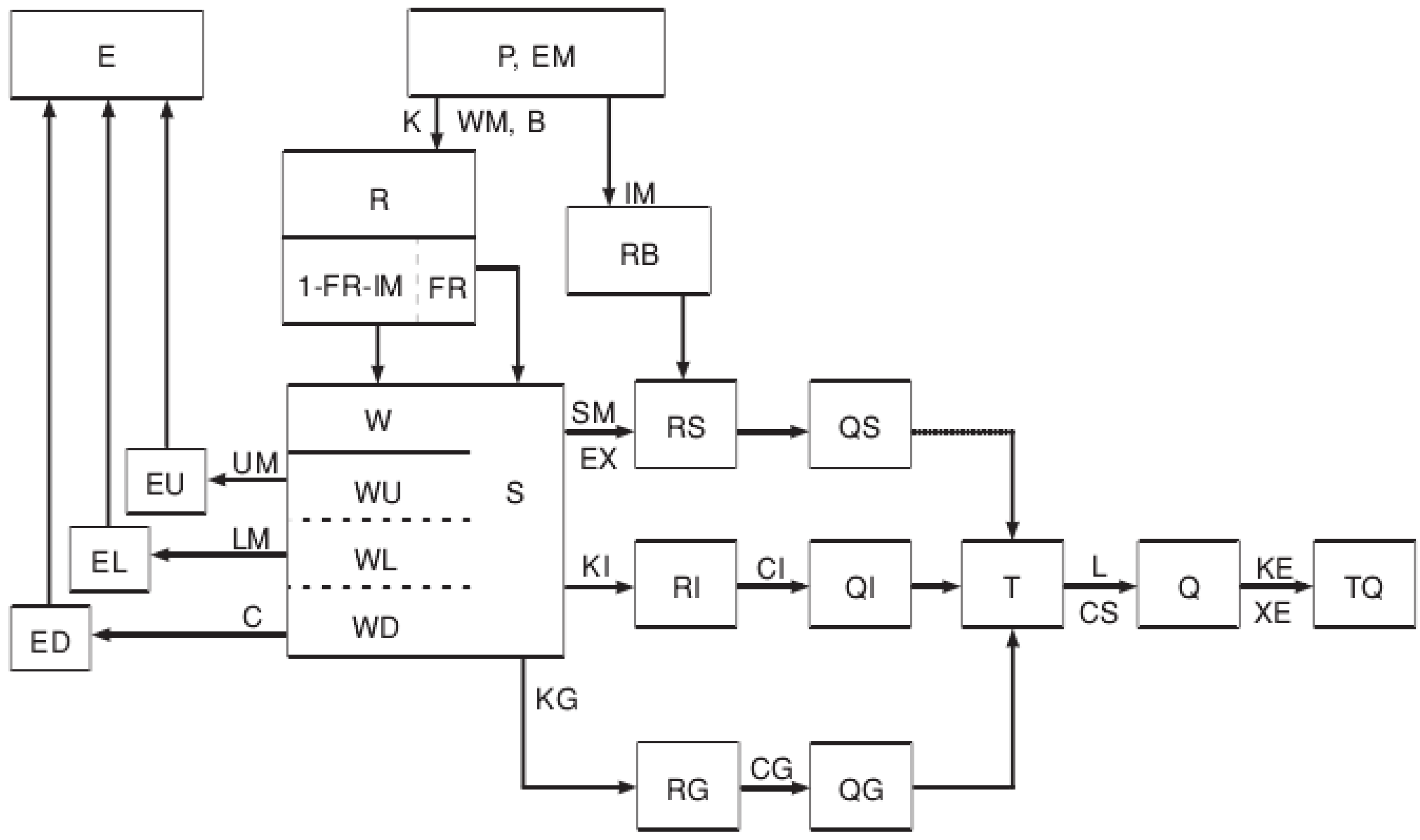
2.3. The Xin’anjiang Hydrological Model
- (1)
- Evapotranspiration. It generates the deficit of soil storage which is divided into the upper, lower and deep layers;
- (2)
- Runoff production. It produces the runoff according to the rainfall and soil storage deficit;
- (3)
- Runoff separation. It divides the total runoff into three components: surface, subsurface and groundwater;
- (4)
- Flow routing. It transfers the local runoff to the outlet of each sub-basin to form the outflow of the sub-basin.
3. Case Study
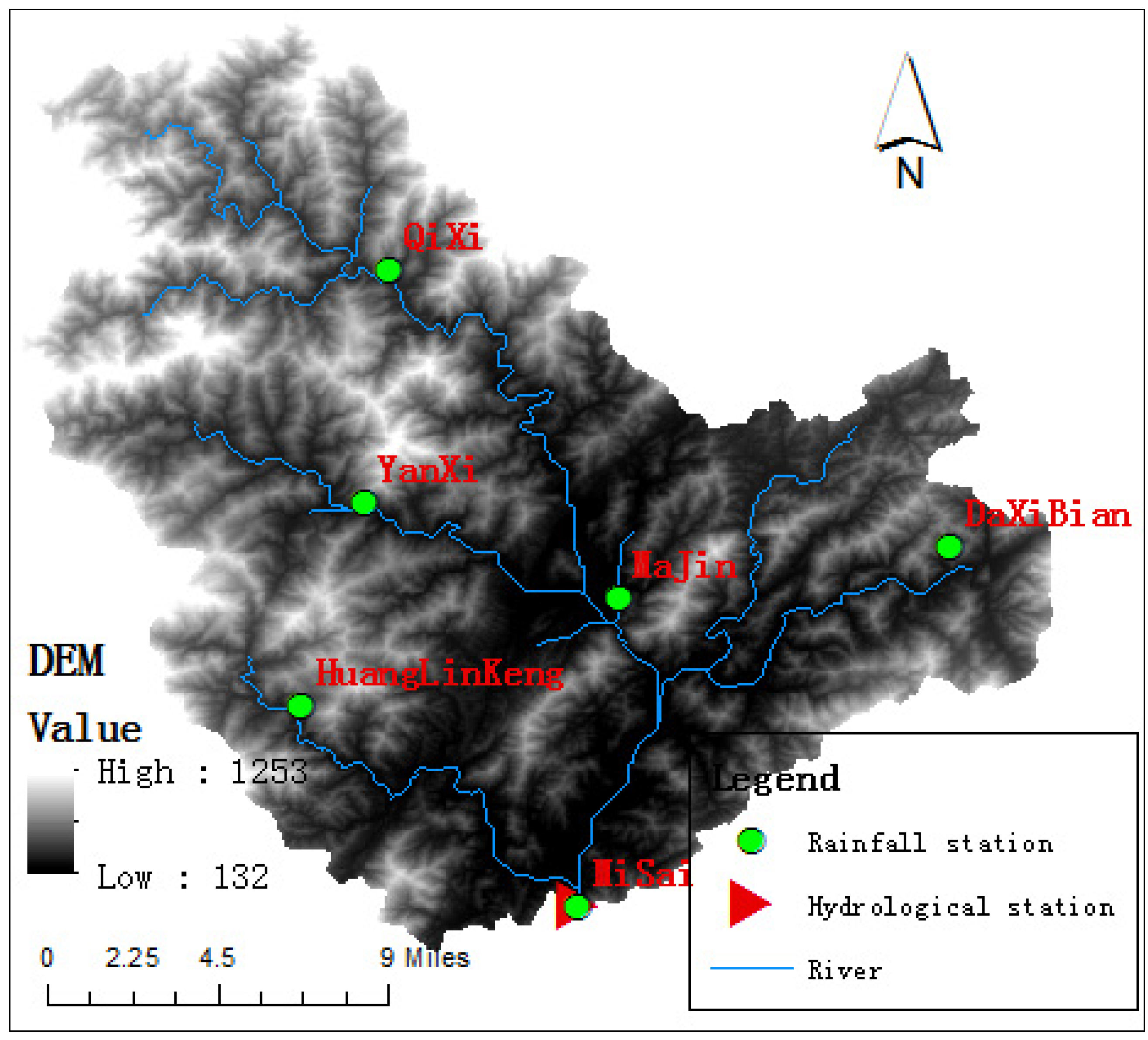
3.1. Study Basin
3.2. Model Implementation
4. Results
4.1. Lead Time of One Hour
4.1.1. Model Parameters
4.1.2. Comparisons
- (1)
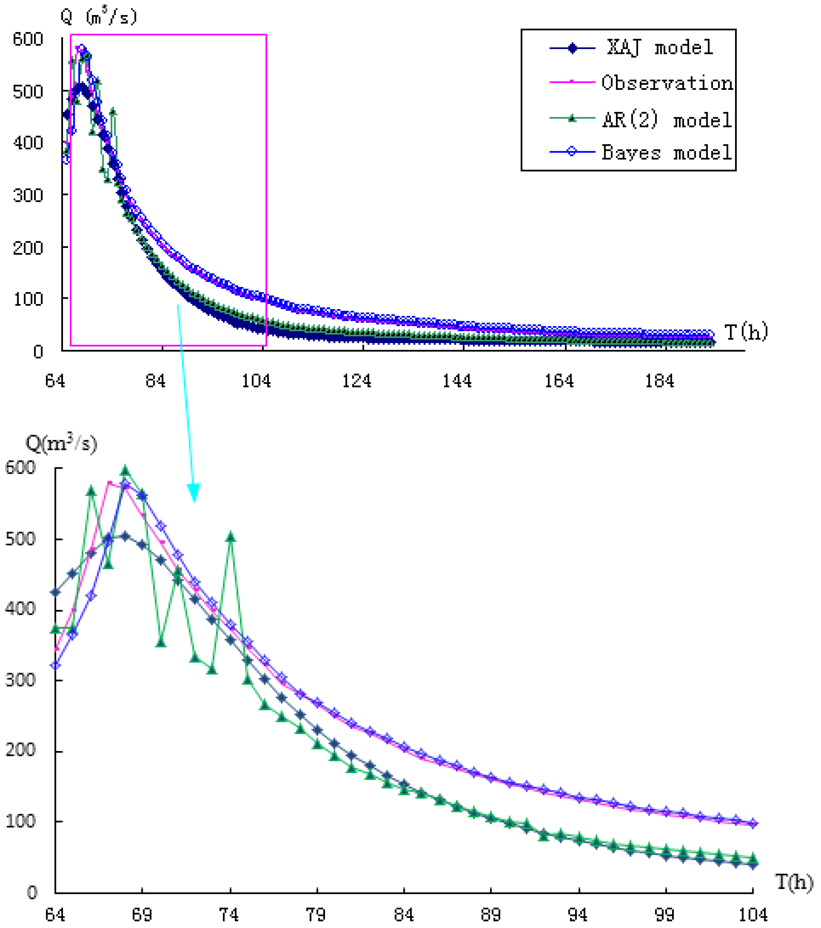
- Flood hygrograph comparison
- (2)
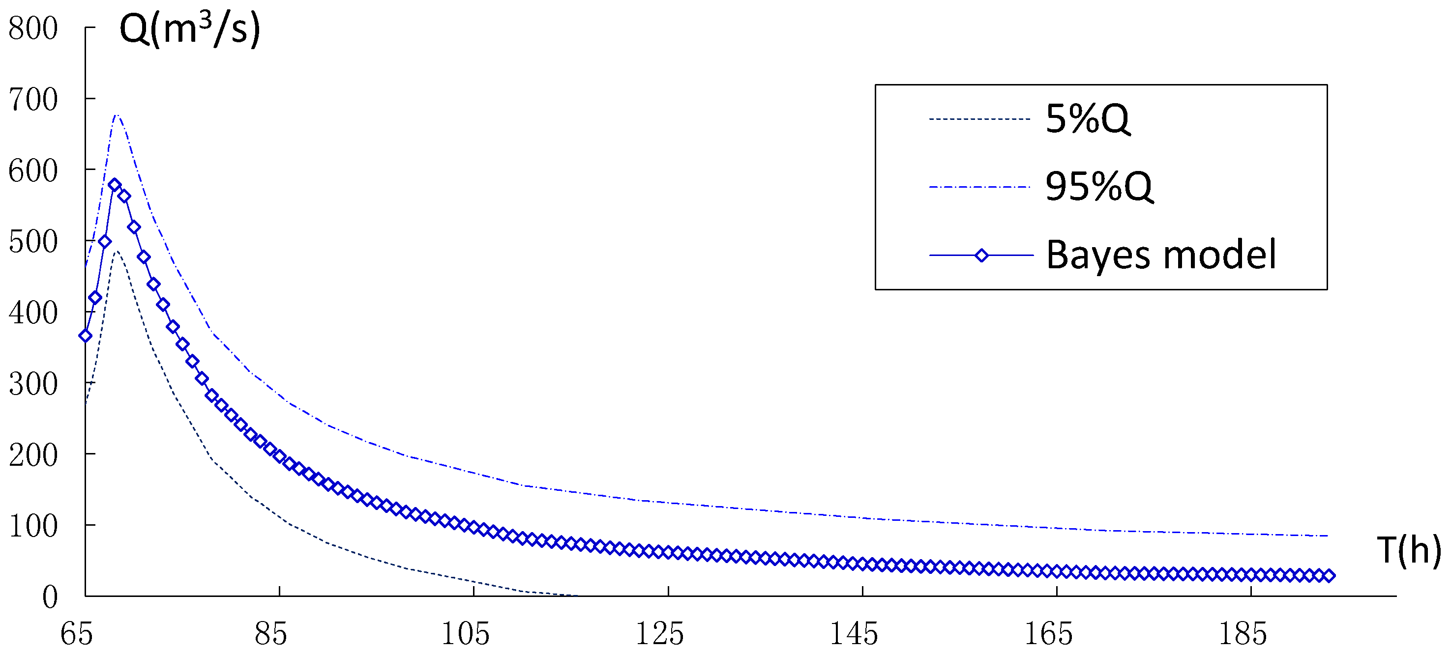
- Quantile and confidence interval results by BSRCM
- (3)
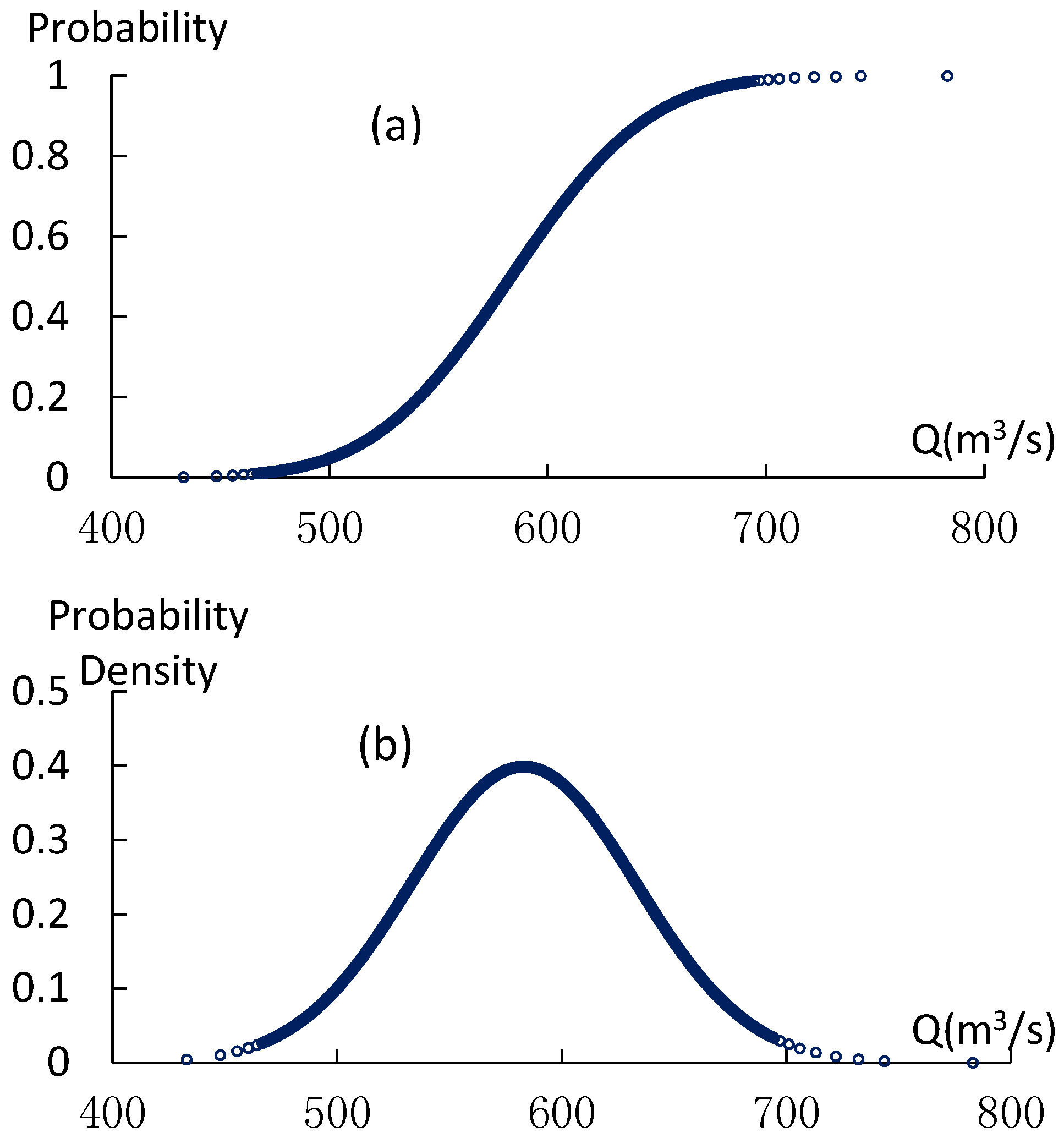
- Posterior density and posterior distribution of flood peak correction results
4.2. Lead Time n > 1 h
4.2.1. Statistical Analysis of Correction Results with Different Lead Times
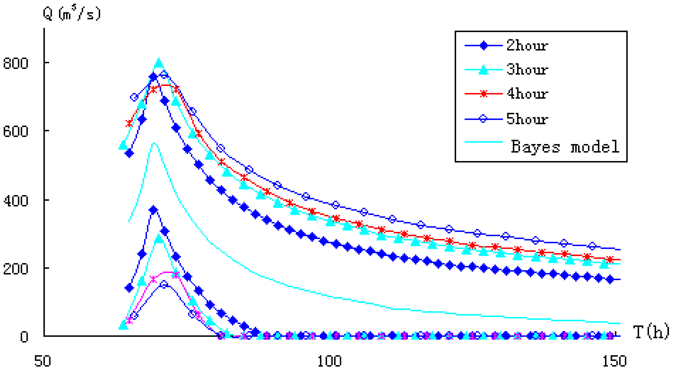
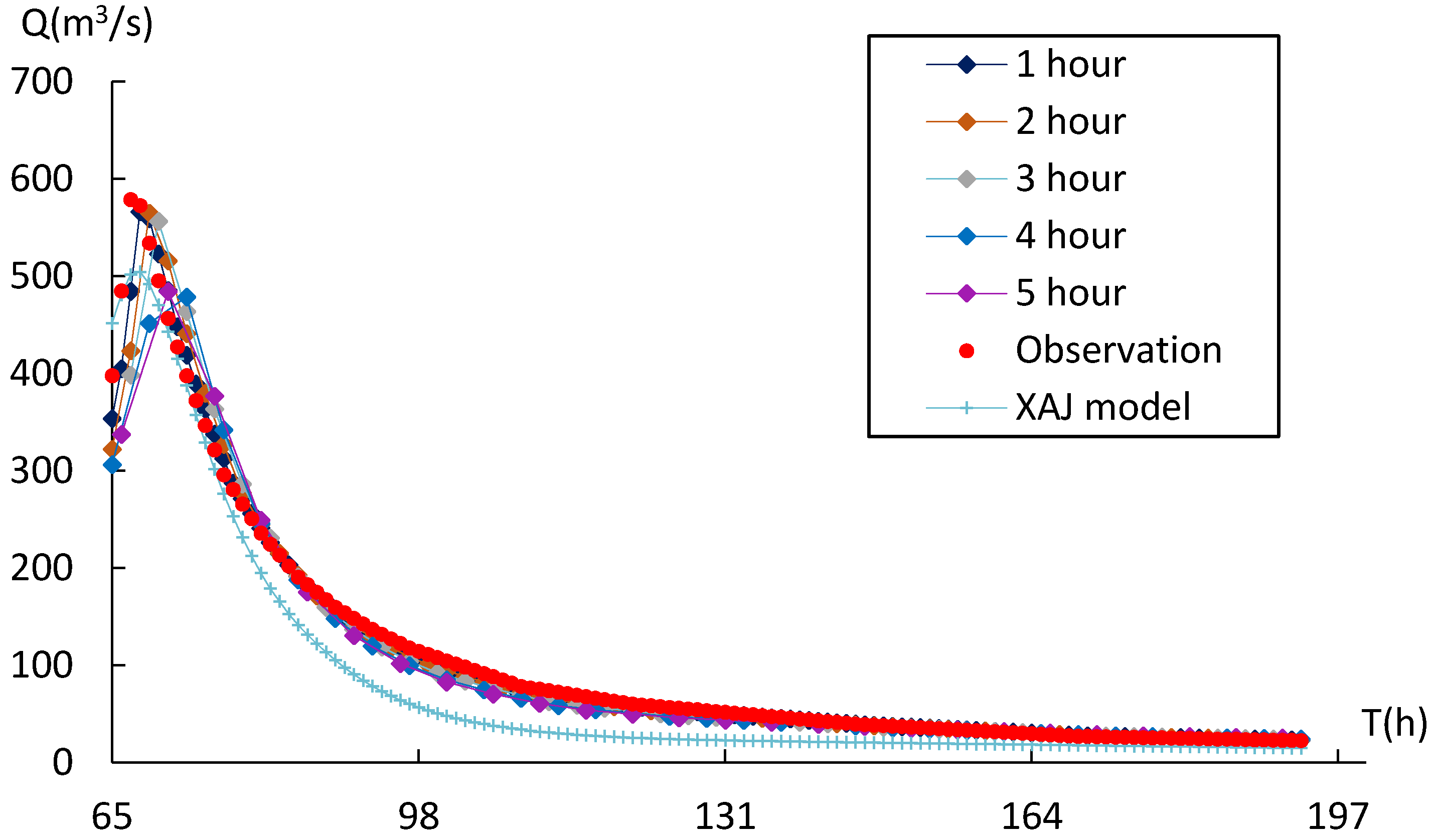
4.2.2. Flood Hygrographs of Different Lead Times
5. Discussion
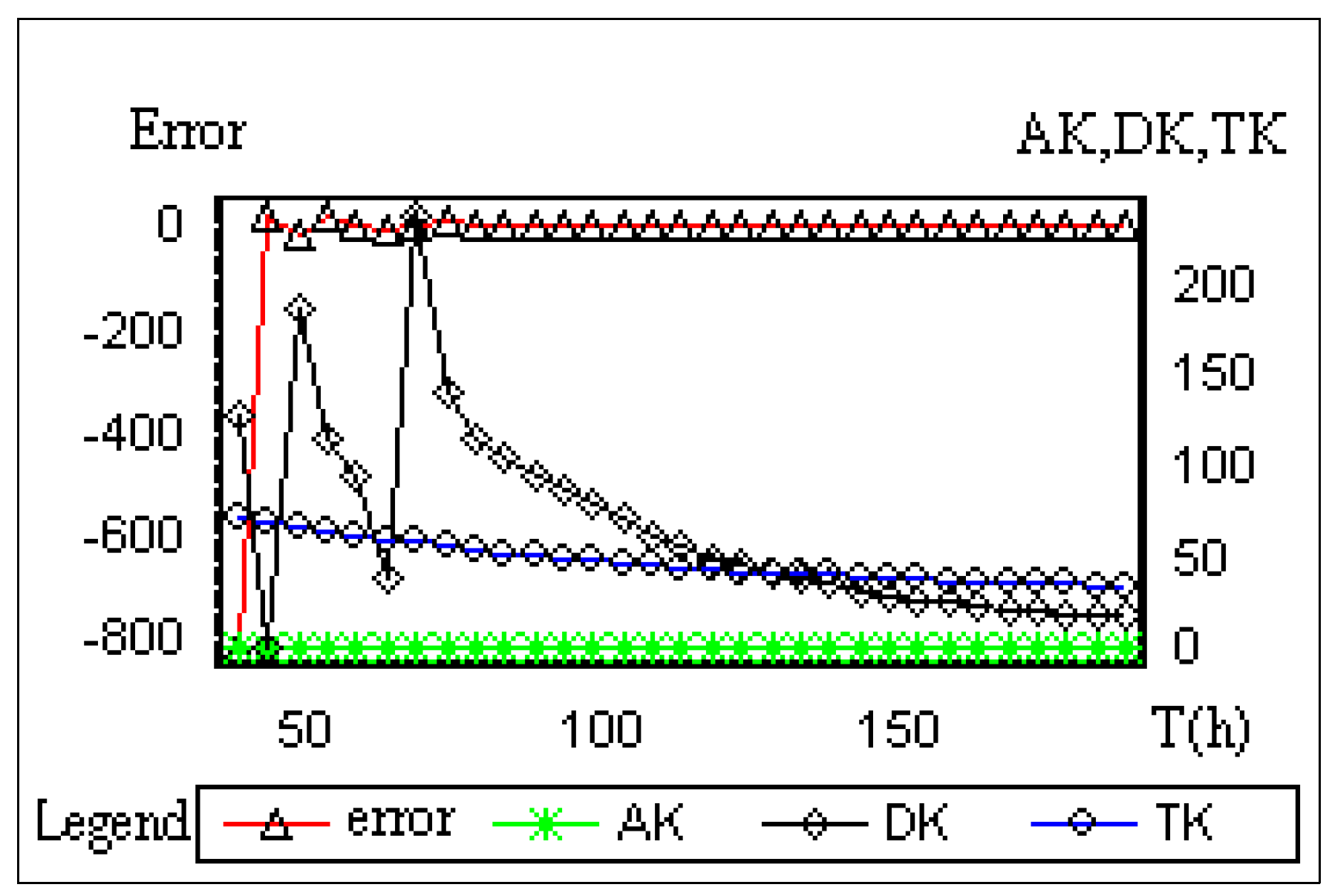
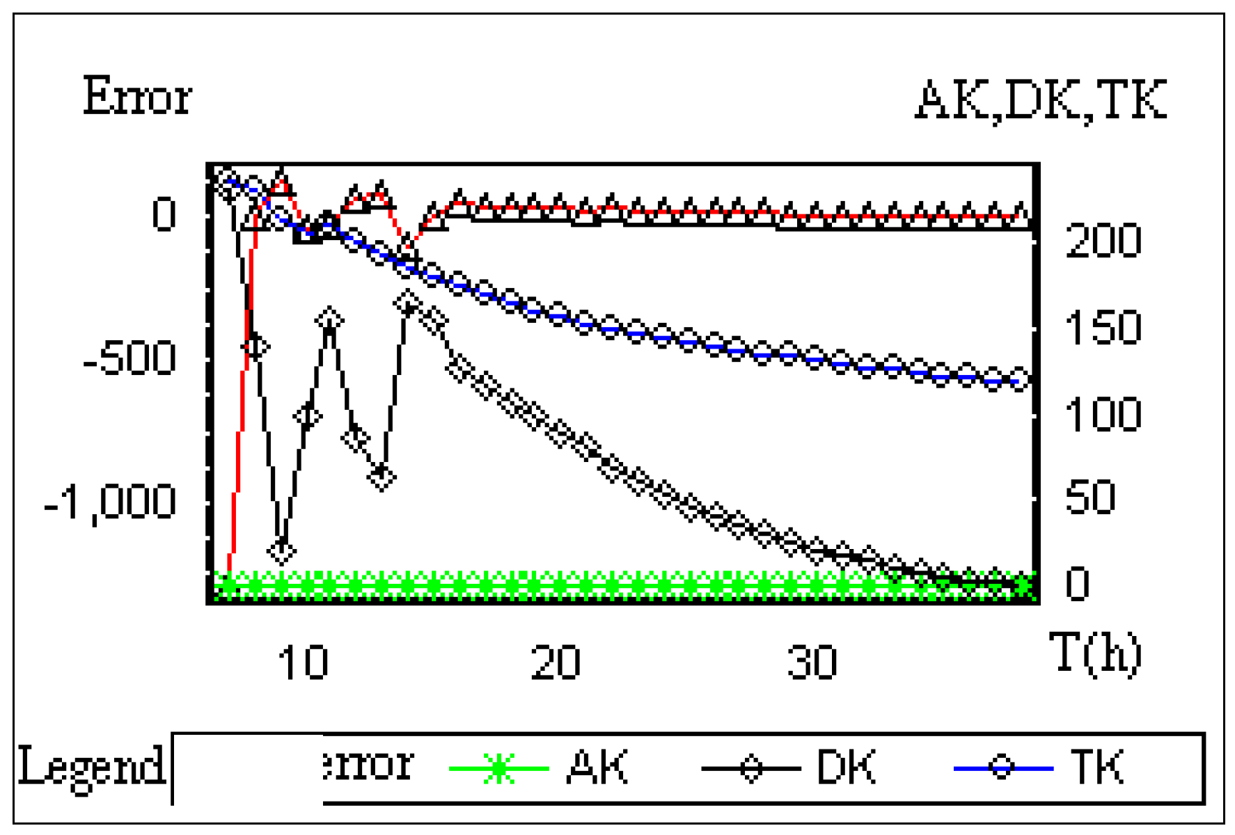
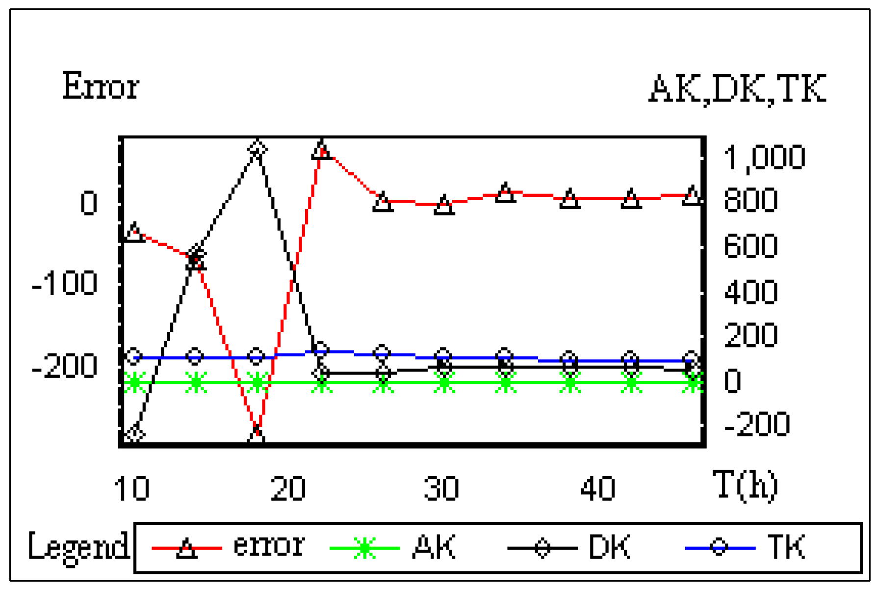
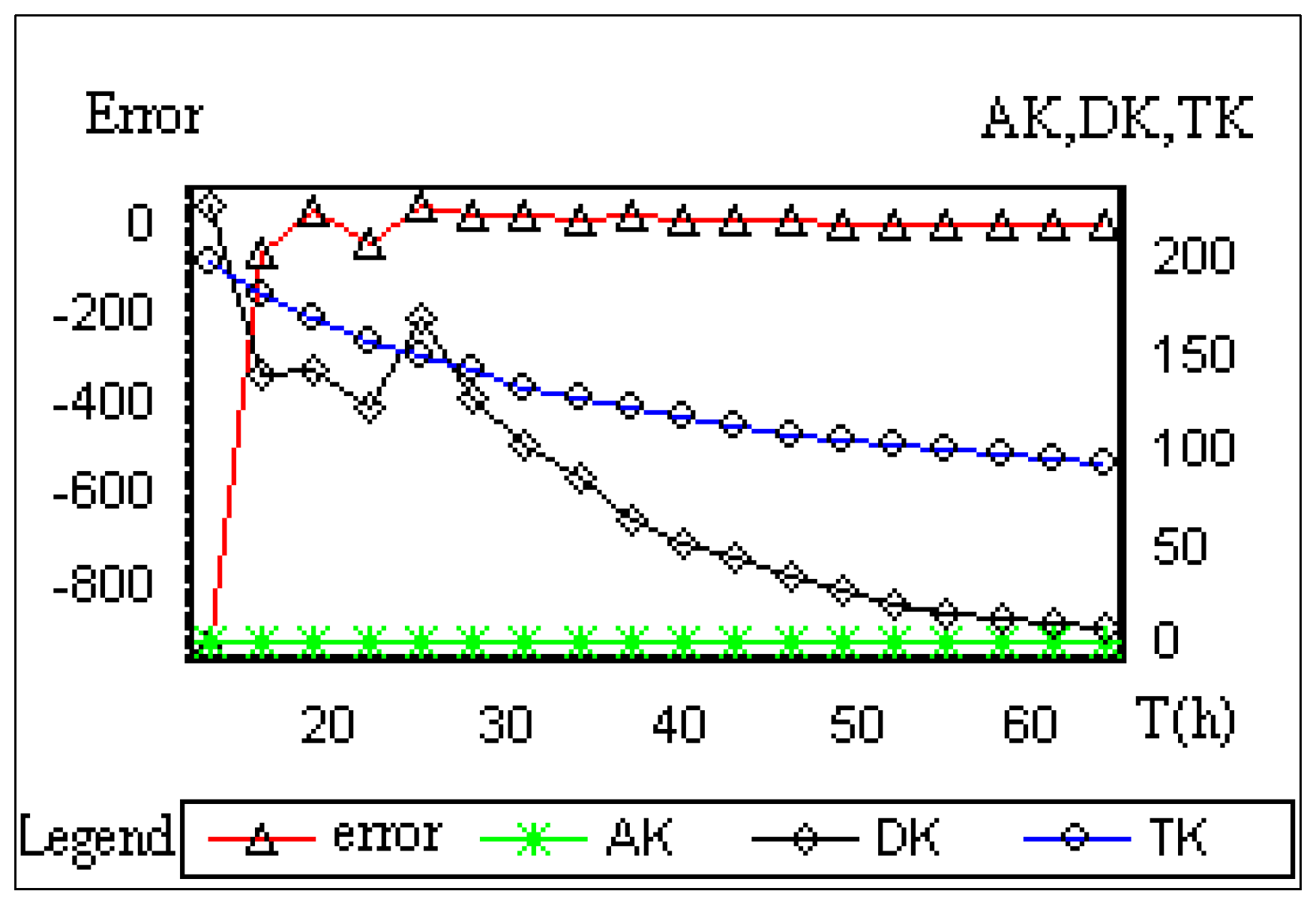
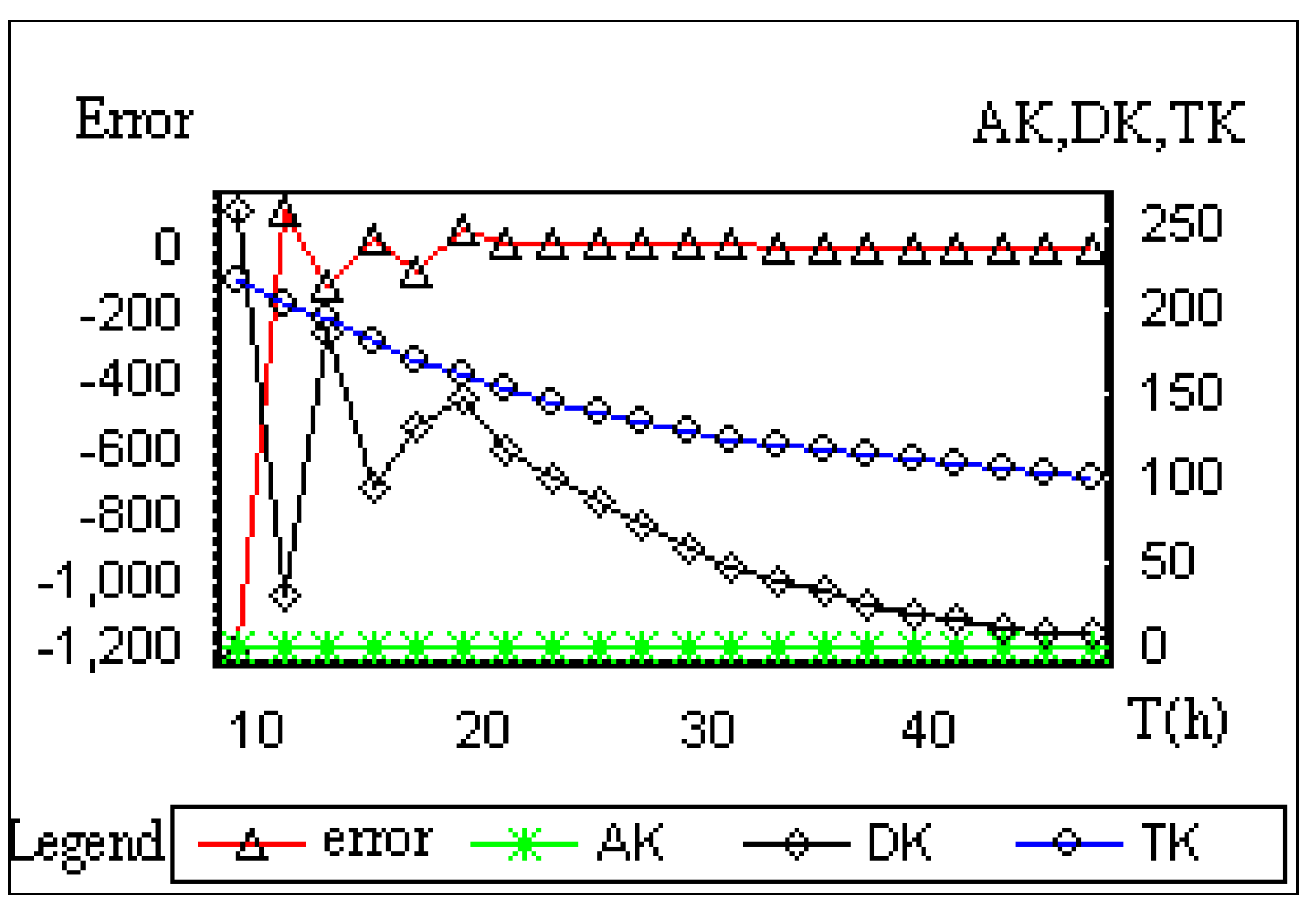
5.1. Parameters and Error Varying with Time Step
5.2. Selection of Model Start-Up Period
6. Conclusions
- (1)
- The BSRCM can increase the precision of flood forecasting and perform well in real-time correction. Results of simulations for nine floods in the Misai basin indicate that, according to the analysis of the determination coefficient, and relative errors of flood volume and flood peak, the BSRCM performed well in the real-time correction and better than the AR(p) model.
- (2)
- The BSRCM provides not only deterministic results but also rich uncertainty information for the forecasting results. The new model can generate the posterior distribution of discharge at any time during the entire flood period. Therefore, the uncertainty information of forecasting results, such as the mean, error variance, variable coefficient, quantile of a specific probability and confidence interval of different confidence levels, can be determined. The uncertainty information could provide more technical support to the local flood control agencies.
- (3)
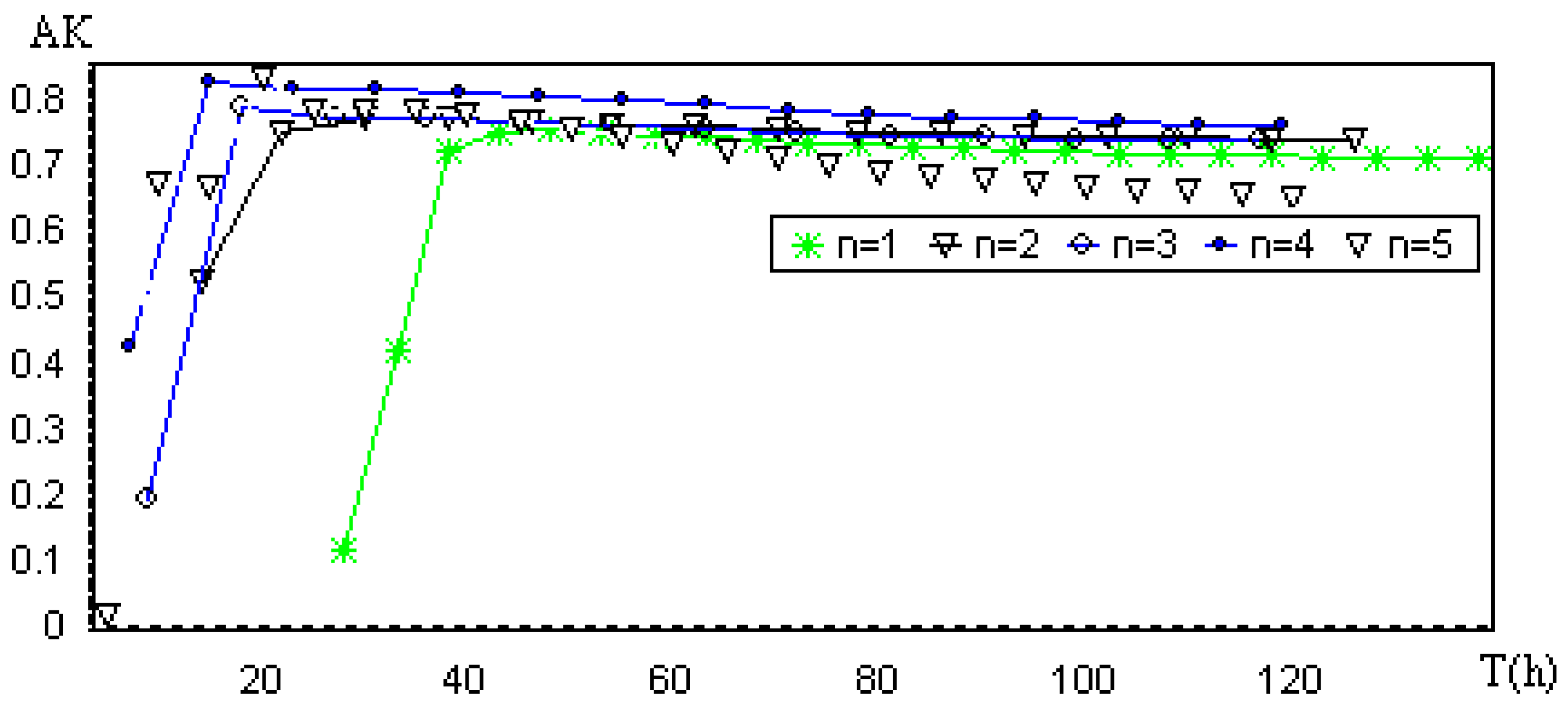
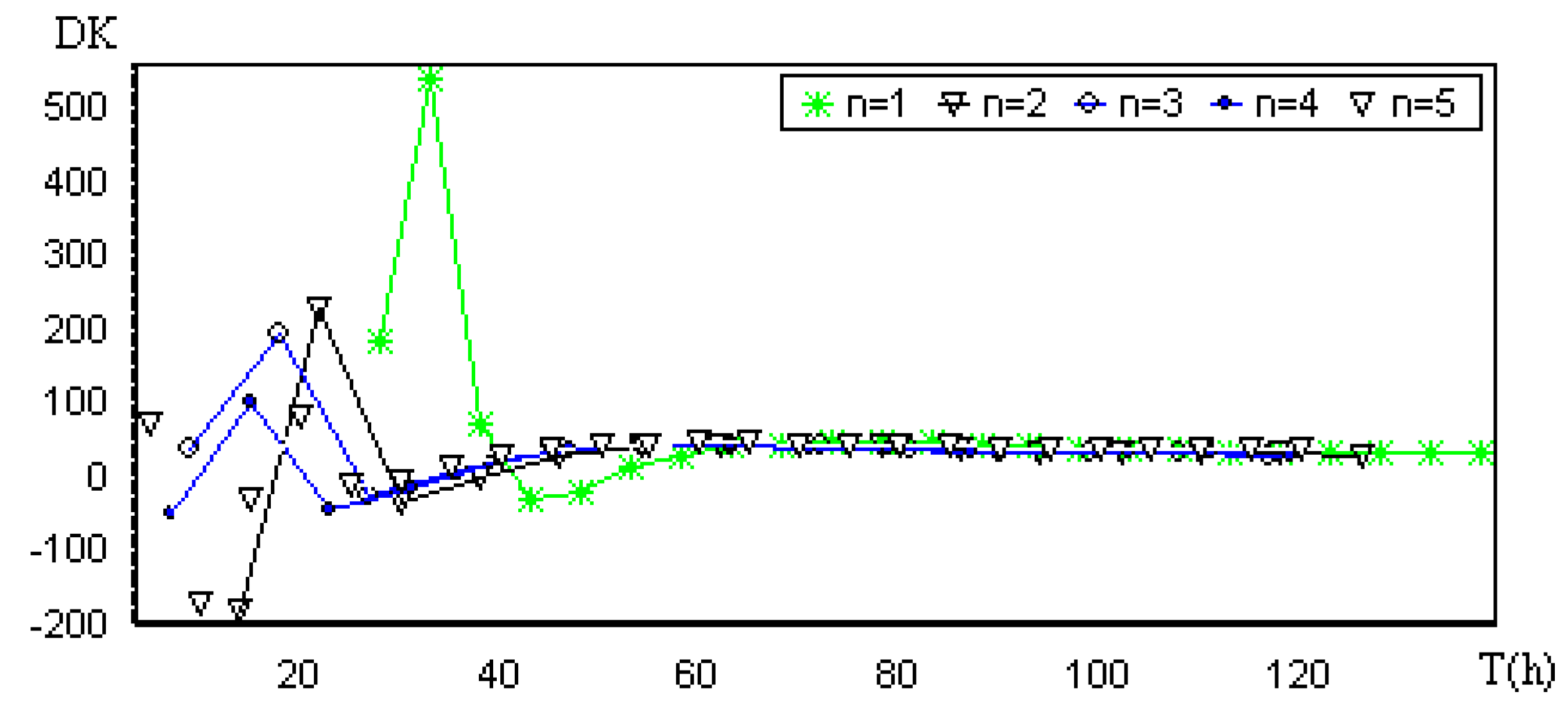
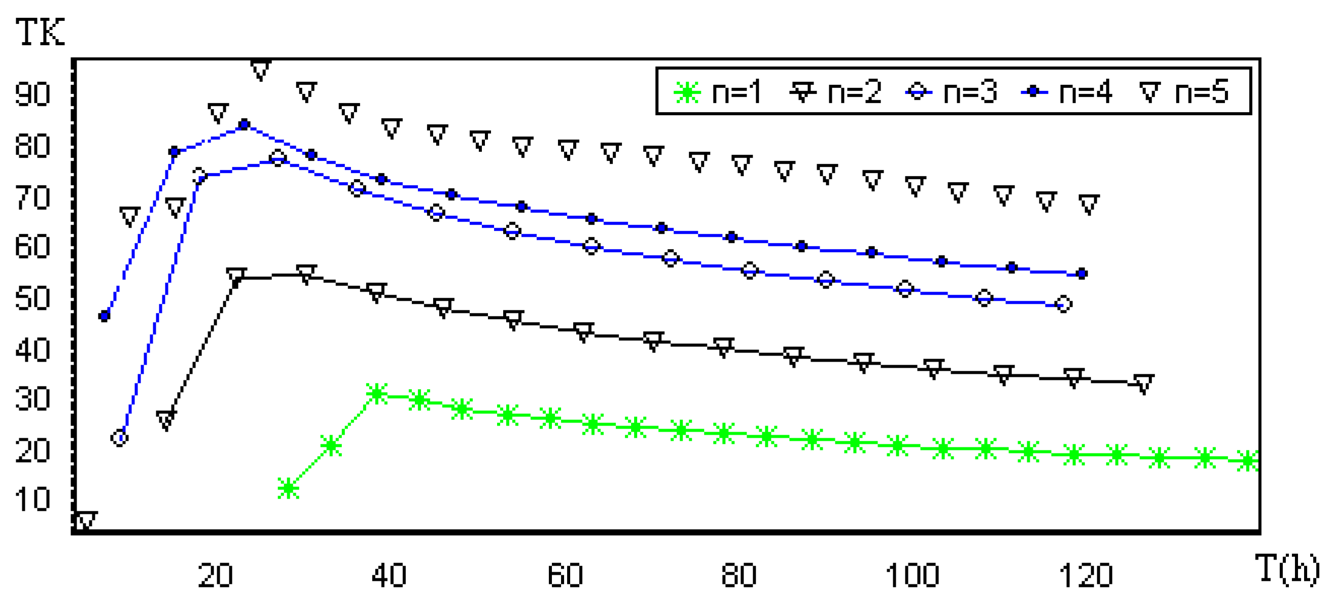
- The BSRCM can achieve good performance with longer lead times. Through the comparisons of the lead time from one to five hours, it was found that the posterior distributions of the three parameters, AK, DK and TK, tend to be more stationary over time with increasing historical information, and the BSRCM with different lead times can predict good results.
Acknowledgments
Author Contributions
Conflicts of Interest
References
- Zhuang, Y.L. Flood Forecasting; Water Resources and Electric Power Press: Wuhan, China, 1995. [Google Scholar]
- Rui, X. New progress of flood forecasting theory and applicability of the existing methods. Water Conserv. Hydropower Sci. Technol. Prog. 2001, 21, 1–4. [Google Scholar]
- Shi, Y.; Davis, K.J.; Zhang, F.; Duffy, C.J.; Yu, X. Parameter estimation of a physically based land surface hydrologic model using the ensemble Kalman filter: A synthetic experiment. Water Resour. Res. 2014, 50, 706–724. [Google Scholar] [CrossRef]
- Li, B.; Yu, Z.; Liang, Z.; Acharya, K. Hydrologic response of a high altitude glacierized basin in the central Tibetan Plateau. Glob. Planet. Chang. 2014, 118, 69–84. [Google Scholar] [CrossRef]
- Beven, K.J.; Kirkby, M.J. A physically based variable contributing model of basin hydrology. Hydrol. Sci. Bull. 1979, 24, 43–69. [Google Scholar] [CrossRef]
- Ciarapica, L.; Todini, E. TOPKAPI: A model for the representation of the rainfall-runoff process at different scales. Hydrol. Processes 2002, 16, 207–229. [Google Scholar] [CrossRef]
- Guo, S. Reservoir Operation Integrated System; Press of Wuhan University of Hydraulic and Electric Engineering: Wuhan, China, 2000. [Google Scholar]
- Arheimer, B.; Lindstrom, G.; Olsson, J. A systematic review of sensitivities in the Swedish flood-forecasting system. Atmos. Res. 2011, 100, 275–284. [Google Scholar] [CrossRef]
- Valipour, M.; Banihabib, M.E.; Behbahani, S.M.R. Comparison of the ARMA, ARIMA, and the autoregressive artificial neural network models in forecasting the monthly inflow of Dez dam reservoir. J. Hydrol. 2013, 476, 433–441. [Google Scholar] [CrossRef]
- Kalman, R. A new approach to linear filtering and prediction theory. Trans. Am. Soc. Mech. Engrs J. Basic Engng Ser. 1960, D82, 35–45. [Google Scholar]
- Kitanidis, P.; Bras, R. Real-time forecasting with a conceptual hydrologic model Analysis of uncertainty. Water Resour. Res. 1980, 16, 1025–1033. [Google Scholar] [CrossRef]
- Georgakaos, K.; Smith, G. On improved hydrologic forecasting results froma WMO real-time forecasting experiment. J. Hydrol. 1990, 114, 17245. [Google Scholar]
- Wu, X.; Wang, C.; Chen, X.; Xiang, X. Kalman filtering correction in real-time forecasting with hydrodynamic model. J. Hydrodyn. 2008, 20, 391–397. [Google Scholar] [CrossRef]
- Takagi, T.; Sugeno, M. Fuzzy identification of system and its application to modeling and control. IEEE Trans. Syst. Man Cybern. 1985, 15, 116–132. [Google Scholar] [CrossRef]
- Nguyen, P.K.T.; Chua, L.H.C. The data-driven approach as an operational real-time flood forecasting model. Hydrol. Process. 2012, 26, 2878–2893. [Google Scholar] [CrossRef]
- Shamseldin, A.; O’Connor, K. A non-linear neural network technique for updating river flow forecasts. Hydrol. Earth Syst. Sci. 2001, 5, 577–597. [Google Scholar] [CrossRef]
- Madsen, H.; Skotner, C. Adaptive state updating in real-time river flow forecasting-a combined filtering and error forecasting procedure. J. Hydrol. 2005, 308, 302–312. [Google Scholar] [CrossRef]
- Wu, S.J.; Lien, H.C.; Chang, C.H.; Shen, J.C. Real-time correction of water stage forecast during rainstorm events using combination of forecast errors. Stoch. Environ. Res. Risk Assess. 2012, 26, 519–531. [Google Scholar] [CrossRef]
- Shen, J.C.; Chang, C.H.; Wu, S.J.; Hsu, C.T.; Lien, H.C. Real-time correction of water stage forecast using combination of forecasted errors by time series models and Kalman filter method. Stoch. Environ. Res. Risk Assess. 2015, 29, 1903–1920. [Google Scholar] [CrossRef]
- Coccia, G.; Todini, E. Recent developments in predictive uncertainty assessment based on the model conditional processor approach. Hydrol. Earth Syst. Sci. 2011, 15, 3253–3274. [Google Scholar] [CrossRef]
- Todini, E. A model conditional processor to assess predictive uncertainty in flood forecasting. Int. J. River Basin Manag. 2008, 6, 123–137. [Google Scholar] [CrossRef]
- Krzysztofowicz, R. Bayesian Forecasting via Deterministic Model. Risk Anal. 1999, 19, 739–749. [Google Scholar] [CrossRef]
- Krzysztofowicz, R.; Karen, K.S. Hydrologic uncertainty processor for probabilistic river stage forecasting. Water Resour. Res. 2000, 36, 3265–3277. [Google Scholar] [CrossRef]
- Krzysztofowicz, R. Bayesian system for probabilistic river stage forecasting. J. Hydrol. 2004, 268, 16–40. [Google Scholar] [CrossRef]
- Krzysztofowicz, R.; Maranzano, C.J. Bayesian system for probabilistic stage transition forecasting. J. Hydrol. 2004, 269, 15–44. [Google Scholar] [CrossRef]
- Herr, H.D.; Krzysztofowicz, R. Bayesian ensemble forecast of river stages and ensemble size requirements. J. Hydrol. 2010, 387, 151–164. [Google Scholar] [CrossRef]
- Li, B.; Yu, Z.; Liang, Z.; Song, K.; Li, H.; Wang, Y.; Zhang, W.; Acharya, K. Effects of climate variations and human activities on runoff in the Zoige alpine wetland in the eastern edge of the Tibetan Plateau. J. Hydrol. Eng. 2014, 19, 1026–1035. [Google Scholar] [CrossRef]
- Zhang, H. Study on probability hydrological forecast system and application based on Bayes theory. Ph.D. Disseration, Wuhan University, Wuhan, China, 2005. [Google Scholar]
- Wang, W.; Ding, J.; Jin, J. Statistical Hydrology; HOHAI University Press: Wuhan, China, 2008. [Google Scholar]
- Zhao, R.; Zhuang, Y.; Fang, L.; Liu, X.; Zhang, Q. The Xin’anjiang Model. In Hydrological Forecasting Proceedings Oxford Symposium; IAHS: Oxford, England, 1980; Volume 129, pp. 351–356. [Google Scholar]
- Singh, V. Computer Models of Watershed Hydrology; Water Resources Publications: Littleton, CO, USA, 1995. [Google Scholar]
- Zhao, R.J. The Xin’anjiang model applied in China. J. Hydrol. 1992, 135, 371–381. [Google Scholar]
- Alazzy, A.A.; Lü, H.; Zhu, Y.H. Assessing the Uncertainty of the Xin’anjiang rainfall-runoff model: Effect of the likelihood function choice on the GLUE method. J. Hydrol. Eng. 2015, 20, 04015016. [Google Scholar] [CrossRef]


| Flood | Total Duration | Starting Time (h) of the Flood Duration (h) | Ck | Ok | X | θ1 | θ2 | χ | AK | DK | TK |
|---|---|---|---|---|---|---|---|---|---|---|---|
| 1 | 192 | 64 | 0.97 | −0.02 | 101.47 | −0.02 | 0.97 | 72.19 | 0.66 | 66.40 | 58.82 |
| 2 | 99 | 33 | 1.02 | −0.22 | 78.95 | −0.22 | 1.02 | 79.17 | 0.50 | 745.00 | 55.90 |
| 3 | 141 | 47 | 0.96 | −0.08 | 57.65 | −0.08 | 0.96 | 33.13 | 0.75 | −25.08 | 28.72 |
| 4 | 165 | 55 | 0.96 | 0.02 | 85.49 | 0.02 | 0.96 | 61.85 | 0.66 | 26.66 | 50.11 |
| 5 | 132 | 44 | 1.03 | −0.42 | 35.86 | −0.42 | 1.03 | 24.62 | 0.68 | 299.53 | 20.30 |
| 6 | 156 | 52 | 0.95 | −0.04 | 32.71 | −0.04 | 0.95 | 30.21 | 0.54 | 68.67 | 22.19 |
| 7 | 192 | 64 | 1.01 | −0.08 | 16.79 | −0.08 | 1.01 | 12.65 | 0.64 | 84.02 | 10.10 |
| 8 | 207 | 69 | 0.93 | 0.06 | 93.94 | 0.06 | 0.93 | 66.55 | 0.67 | 63.07 | 54.30 |
| 9 | 144 | 48 | 0.98 | 0.00 | 94.35 | 0.00 | 0.98 | 67.87 | 0.66 | 429.18 | 55.10 |
| Flood | Relative Error of Flood Volume Error BSRCM/AR(2) | Relative Error of Flood Peak BSRCM/AR (2) | Coefficient of Determination BSRCM/AR (2)/Xin’anjiang Model | Flood Peak Lag Time BSRCM/AR (2)/Xin’anjiang Model | ||||||
|---|---|---|---|---|---|---|---|---|---|---|
| 1 | 0.05 | 0.02 | 0.16 | 0.09 | 0.99 | 0.96 | 0.91 | 1 | 1 | 1 |
| 2 | 0.04 | 0.18 | −0.01 | −0.01 | 0.98 | 0.98 | 0.89 | 0 | 0 | −1 |
| 3 | 0.09 | 0.21 | 0.02 | 0.02 | 0.97 | 0.85 | 0.74 | −1 | −1 | −1 |
| 4 | 0.02 | 0.14 | 0.01 | −0.14 | 0.99 | 0.89 | 0.88 | 0 | 0 | 0 |
| 5 | 0.10 | −0.02 | 0.10 | −0.04 | 0.99 | 0.98 | 0.94 | 1 | 1 | 1 |
| 6 | 0.06 | 0.15 | 0.01 | 0.06 | 0.99 | 0.95 | 0.6 | 0 | 0 | −1 |
| 7 | 0.08 | 0.16 | 0.06 | 0.01 | 0.99 | 0.95 | 0.75 | 0 | 0 | 0 |
| 8 | −0.02 | 0.07 | −0.02 | −0.10 | 0.99 | 0.98 | 0.9 | 0 | 1 | 1 |
| 9 | 0.04 | −0.12 | 0.01 | −0.14 | 0.98 | 0.9 | 0.91 | 0 | 0 | 1 |
| Lead Time (h) | 1 | 2 | 3 | 4 | 5 | |
|---|---|---|---|---|---|---|
| Flood ID | ||||||
| 19820619 | 0.99 | 0.98 | 0.97 | 0.96 | 0.93 | |
| 19830529 | 0.98 | 0.95 | 0.93 | 0.91 | 0.85 | |
| 19830614 | 0.97 | 0.98 | 0.98 | 0.97 | 0.94 | |
| 19830620 | 0.99 | 0.99 | 0.98 | 0.94 | 0.96 | |
| 19840402 | 0.99 | 0.98 | 0.98 | 0.99 | 0.99 | |
| 19850703 | 0.99 | 0.98 | 0.97 | 0.95 | 0.91 | |
| 19860704 | 0.99 | 0.98 | 0.99 | 0.96 | 0.98 | |
| 19870620 | 0.99 | 0.98 | 0.96 | 0.95 | 0.92 | |
| 19880621 | 0.98 | 0.95 | 0.93 | 0.90 | 0.93 | |
| Forecast Lead Time (h) | Starting Time | Relative Error of Flood Volume (%) | Relative Error of Peak Discharge (%) | Error of Flood Peak Time (h) | Deterministic Coefficient |
|---|---|---|---|---|---|
| 1 | One third of flood duration | −0.01 | −0.02 | 1 | 0.99 |
| 2 | 0.01 | −0.08 | 1 | 0.98 | |
| 3 | 0.01 | −0.08 | 1 | 0.97 | |
| 4 | 0.03 | −0.16 | 1 | 0.96 | |
| 5 | 0.04 | −0.22 | 1 | 0.93 | |
| 1 | One fourth of flood duration | −0.01 | −0.02 | 1 | 0.99 |
| 2 | −0.01 | −0.08 | 1 | 0.98 | |
| 3 | 0.01 | −0.08 | 1 | 0.96 | |
| 4 | 0.02 | −0.16 | 1 | 0.95 | |
| 5 | 0.05 | −0.22 | 1 | 0.92 | |
| 1 | One fifth of flood duration | 0.01 | 0.01 | 1 | 0.99 |
| 2 | −0.01 | 0.01 | 1 | 0.97 | |
| 3 | −0.02 | −0.08 | 1 | 0.95 | |
| 4 | 0.01 | −0.16 | 1 | 0.95 | |
| 5 | 0.01 | −0.19 | 1 | 0.93 | |
| 1 | One sixth of flood duration | −0.01 | 0.01 | 1 | 0.98 |
| 2 | −0.02 | 0.01 | 1 | 0.93 | |
| 3 | 0.01 | −0.08 | 1 | 0.95 | |
| 4 | 0.05 | −0.16 | 1 | 0.93 | |
| 5 | 0.01 | −0.19 | 1 | 0.88 |
© 2016 by the authors; licensee MDPI, Basel, Switzerland. This article is an open access article distributed under the terms and conditions of the Creative Commons by Attribution (CC-BY) license (http://creativecommons.org/licenses/by/4.0/).
Share and Cite
Wang, J.; Liang, Z.; Jiang, X.; Li, B.; Chen, L. Bayesian Theory Based Self-Adapting Real-Time Correction Model for Flood Forecasting. Water 2016, 8, 75. https://doi.org/10.3390/w8030075
Wang J, Liang Z, Jiang X, Li B, Chen L. Bayesian Theory Based Self-Adapting Real-Time Correction Model for Flood Forecasting. Water. 2016; 8(3):75. https://doi.org/10.3390/w8030075
Chicago/Turabian StyleWang, Jun, Zhongmin Liang, Xiaolei Jiang, Binquan Li, and Li Chen. 2016. "Bayesian Theory Based Self-Adapting Real-Time Correction Model for Flood Forecasting" Water 8, no. 3: 75. https://doi.org/10.3390/w8030075
APA StyleWang, J., Liang, Z., Jiang, X., Li, B., & Chen, L. (2016). Bayesian Theory Based Self-Adapting Real-Time Correction Model for Flood Forecasting. Water, 8(3), 75. https://doi.org/10.3390/w8030075