Article

A Study of Energy Optimisation of Urban Water Distribution Systems Using Potential Elements

Department of Building Services Engineering, Polytechnic University of Timisoara, Piata Bisericii 4A, 300233 Timisoara, Romania
Water 2016, 8(12), 593; https://doi.org/10.3390/w8120593
Submission received: 29 October 2016 / Revised: 25 November 2016 / Accepted: 5 December 2016 / Published: 14 December 2016
(This article belongs to the Special Issue Water Supply and Drainage for Sustainable Built Environment)

Abstract

:
Energy use in water supply systems represents a significant portion of the global energy consumption. The electricity consumption due to the water pumping represents the highest proportion of the energy costs in these systems. This paper presents several comparative studies of energy efficiency in water distribution systems considering distinct configurations of the networks and also considers implementation of the variable-speed pumps. The main objective of this study is the energy optimisation of urban systems using optimal network configurations that reduce energy consumption and improve energy efficiency. The paper describes in detail four strategies for improving energy efficiency of water pumping: control systems to vary pump speed drive according to water demand, pumped storage tanks, intermediary pumping stations integrated in the network, and elevated storage tanks floating on the system. The improving energy efficiency of water pumping is briefly reviewed providing a representative real case study. In addition, a different approach for the hydraulic analysis of the networks and the determination of the optimal location of a pumped storage tank is provided. Finally, this study compares the results of the application of four water supply strategies to a real case in Romania. The results indicate high potential operating costs savings.

1. Introduction

As a vital part of water supply systems, water distribution networks represent one of the largest infrastructure assets of industrial society. According to Watergy [1], approximately 2% to 3% of the worldwide electricity consumption is used for pumping in water supply systems, while 80%–90% of this consumption is absorbed by motor-pump sets [2]. Coelho and Andrade-Campos [3] provides several strategies to improve the energy efficiency of the water supply systems.
Most water distribution systems require the operation of pumps to deliver the necessary quantity of water with the adequate pressure to the final consumers. As reported by Bene et al. [4] and Vilanova and Balestieri [5], the electricity used to pump water is a significant part of the total operation in water supply systems.
Water distribution systems equipped with pumping stations are characterised by energy consumption greater than 60% of the energy consumed by the operation of the entire supply system of large urban centres [6]. As a result, a great increase in the energetic system load occurs especially during peak water consumption hours.
Pumping systems are found to have a significant potential for energy efficiency improvements [7,8,9,10]. In most cases, optimisation of operations has only considered fixed speed pumps and the cost savings that may be obtained by exploiting a multi-pattern electric tariff [11,12,13,14,15]. Pump and motor upgrades to more efficient solutions, either being technologically more advanced or because they are more properly adjusted to the system, often allow significant energy savings [2].
Vogelesang [16] quantitatively discussed the energy saving potential of applying variable-speed pumps and indicated a possible energy reduction of 27% only with a 10% of pump speed decrease. Variable-speed drives (VSDs) have been shown to be an effective way to reduce the pumping energy, especially in systems that require a wide range of flow rates [17] in absence of elevated tanks. Energy optimisation of parallel-connected, rotational speed-controlled pumps has been studied to some extent [18,19]. Viholainen et al. [20] developed a pumping control strategy for most of the scenarios considered (two pumps in parallel, two frequency converters, and one programmable logic controller) using frequency converters that close to high efficiency.
Several studies provide other alternatives to improve energy efficiency in water distribution systems. A model for decision systems regarding the quantification, location and opening adjustment of control valves in a distribution network, to minimize pressures and leakage levels in network is developed in [21]. Carravetta et al. [22] present a real case study (flow rate less than 1440 m3/h) and suggest the installation of pumps in the supply pipes that act as micro-hydro turbines to generate electric power. These turbines may be used to provide pressure control instead of using pressure control valves.
Diniz et al. [23] present an analysis of energy efficiency in supply systems based on modelling and optimisation. Other researchers have successfully applied genetic algorithms to control hydraulic pressure in the water distribution network [24]. However, these models require that the functions satisfy certain restrictive conditions that cannot be generally guaranteed for any water distribution system.
The assessment of energy efficiency in water distribution systems is strongly influenced by the site-dependent nature of the water-energy nexus in pressurised networks [25]. Understanding this link requires a systematic energy analysis to separately evaluate the influence of pumping stations, the network and water loss and to highlight inconsistencies in the design and management that are reflected in both of the resources, namely water and energy.
The hourly variations in water demand during the day are much greater compared to the average daily demand. For a domestic consumer water requirement is more during morning and evening hours than the noon demand. The hourly variation in demand has also an influence on the residual pressures in the system. In the case of water distribution for Romanian consumers, the available pressure is greater at the periphery consumers, where the lower pressure is necessary, while in central zones, the pressure is insufficient. Often, the absence of water at consumers can be observed during certain hours in a 24-h period due to system under dimensioning, increased water consumption by some users, inadequate operation of pumping stations, or a combination of these factors. These disadvantages are amplified by the overlapping of peak hours for water, heat, and electricity consumption, especially between 7:00 and 9:00 in the morning and between 17:00 and 21:00 in the evening, contributing to increasing operation expenses.
During peak hours, the energy cost is 2–3 times more expensive than during the hours of minimum consumption. Therefore, it is very interesting to provide a reduction of energy consumption during peak hours. A technical solution for this reduction can be a decrease in the pumping power (even stopping pumps if it is possible) during peak hours, along with an extensive delivery outside of these hours. Consequently, distribution systems must be equipped with pumped storage tanks.
An important goal is the absolute reduction of pumping energy, which is possible by dividing the system into zones. For this purpose, a special form of parallel zoning procedure or a vertical division into zones with intermediary pumps mounted on the distribution mains, or a combined solution with more potential elements, can be used [26].
In this context, this paper presents several comparative studies of energy efficiency in water distribution systems considering distinct configurations of the networks and also considers utilisation of the variable-speed pumps. The main aim of the paper is to search for possible optimal network configurations that reduce electricity consumption and improve energy efficiency using potential elements (pumped storage tanks, intermediary pumping stations integrated on distribution mains, elevated storage tanks floating on the system) and control systems to vary pump speed drive according to water demand. The improving energy efficiency of water pumping is briefly reviewed providing a representative real case study. In addition, a hydraulic analysis of the optimisation strategies with potential elements is performed and an analytical model is developed to estimate the optimal location of a pumped storage tank. Finally, certain optimisation solutions to reduce pumping energy are analysed in a detailed manner through the use of a case study to ascertain their energy and economic efficiencies.

2. Improving Energy Efficiency of Water Pumping

2.1. A Brief Review of Previous Works

Some pumping stations comprise parallel-connected pumps with fixed-speed and flow rate controlled by the number of pumps in operation. In this procedure, it is very difficult to define a pumps operating schedule with minimal energy cost without compromising the full delivery of daily demand and ensuring a suitable reservoir level for the next work cycle. According to Feldman [27], the main improvements in energy efficiency can be obtained with: (1) pumping stations and system design improvement; (2) VSDs installations; (3) efficient operation of pumps; and (4) minimisation of water losses through pressure control.
The power absorbed by a pump in a water supply system P, in W, and the electricity consumption W, in Wh, can be calculated using following equations:
P = γ Q H p η
W = P T p
where γ is the water specific weight, in N/m3; Q is the pump discharge, in m3/s; Hp is the pump head for the operating point, in m; η is the global efficiency of the pumping station; and Tp is the operation period, in h.
The specific energy consumption w, in %, for an optimal operation period Tp of the pumps can be estimated as:
w = 0 T p P d t i = 1 24 Q i H i η i γ T p 100
where Qi, Hi, and ηi are the pump characteristics in classical operation at the ith hour of a day; and 0 T p P d t is the energy consumption during interval Tp at discharges different from Qi.
Most existing pumping stations requiring flow control make use of bypass lines, throttling valves, or pump speed adjustments.
Most water distribution systems are fed through some type of centrifugal pumps characterized by a head–flow (H-Q) curve. A centrifugal pump has a motor that spins a piece within the pump called an impeller. If the pump used is a fixed-speed pump, the operating point is forced to move along the pump curve corresponding to the constant nominal speed. There are two methods to adjust the water flow rate in a pipe network with a fixed-speed pump:
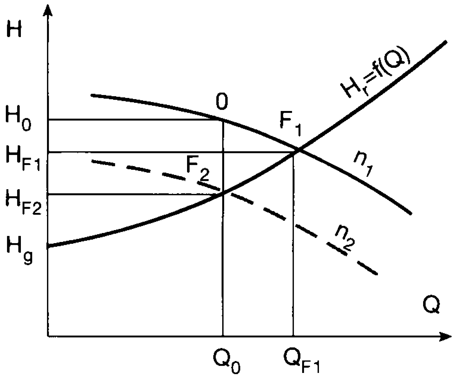
  • Bypassing part of the water flow rate.
  • Introducing a supplementary pressure loss using a control valve [28] that can lead to higher energy efficiency of the water supply system when the nominal pump head is lower than the optimal value. Additionally, valves can be a source of emissions and suffer from corrosion, erosion, plugging, cavitation, and leakage.
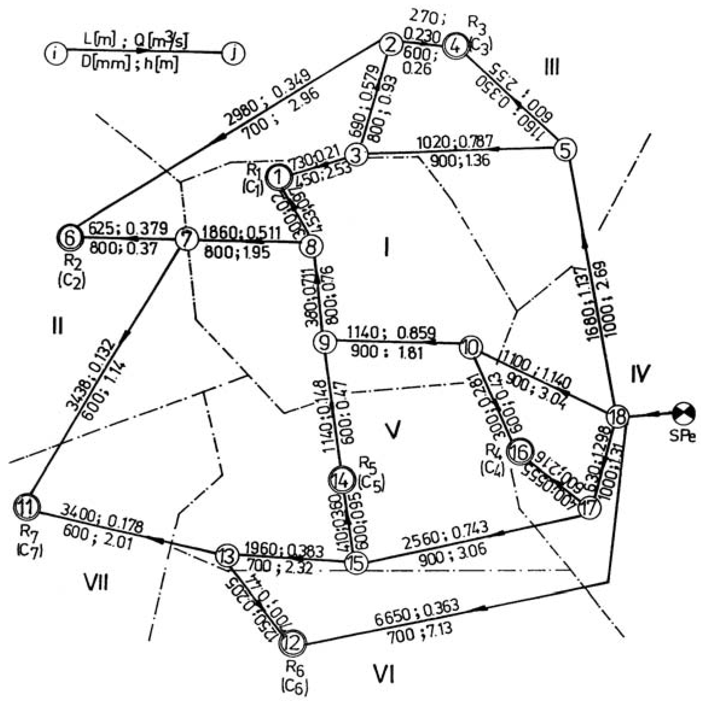
Speed can be controlled in a number of ways, either the most popular type of VSD being the variable frequency drive (VFD) or variable-speed controller.
Using VSDs to replace fixed-speed pumps has the possibility to save electrical energy. The decreasing energy consumption can be reduced the cost related to pump operation. Variable-speed pumps can prevent over-pressurising of the water distribution system that has no storage floating on the system (that is, no tank where the hydraulic grade line (HGL) in the tank is the same as the HGL in the system) [6].
Variable-speed pumps are coupled with a motor that is controlled by a VFD. The most common form of VFD is the voltage-source, pulse-width modulated (PWM) frequency converter. The principal duty of the VFD is to alter the main supply to vary the speed of the motor while delivering the required torque at higher efficiency. As a result, as the pump speed changes, the pump curve is adjusted for different operating conditions. The flow control (Figure 1) is achieved by changing the pump curve H (at different pump speeds n1 and n2) on the fixed system curve Hr. Pipe work curve Hr start from point (0, Hg), where Hg is the geodesic head. The operating point F2 corresponds to the reduced pump head HF2.
The approximation introduced into the power-speed relation implies that the efficiency will remain constant for speeds n1 and n2, i.e., that the efficiency curve will only be shifted to the left in the case of speed reduction. The efficiency variation depending of the pump speed is provided by following analytical relationship [29]:
η 2 = 1 ( 1 η 1 ) ( n 1 n 2 ) 0.1
where n1 and n2 are two different speeds and η1, η2 are the corresponding efficiencies.
Therefore, as indicated in [30], for the particularly case of the large pumps the changes in efficiency can be neglected if the changes in speed rate do not exceed 1/3 from the nominal pump speed. Figure 2 shows the variation curves of pump head (H), flow rate (Q), power (P), and efficiency (η) for centrifugal pumps depending on pump speed n. It can be observed that a reduction of 20% of the pump speed will lead to the decreasing of power demand of 50% at constant pump efficiency. Thus, the possibility exists to reduce the pumping energy consumption by using VSDs.
Variable-speed pumps are useful in applications requiring operational flexibility, such as when flow rates change rapidly, but the required pressure remains constant [6]. These pumps can take advantage of the different required operating conditions in water distribution systems. In particular, the reduction in energy consumption exploits the possibility of reducing the head or flow rate in the system. Figure 1 shows the case in which the required flow rate is smaller than the actual operating point. This situation can be the case of a water transmission system, where the pumps are used to move water from a lower to an upper tank. Because the pumping at a particular time of the year may be sized for a peak-day demand, the pump will deliver a flow rate associated with the operating point, despite the fact that the required demand is decreased. However, this operating strategy can be economically convenient if the system has a sufficient storage volume so that pumps can be switched on only during the off-peak-tariff period.
Parallel-connected centrifugal pumps are often implemented in the pumping systems with a widely varying flow rate demand [31,32]. The output of the parallel-connected centrifugal pumps in a system can be adjusted with an on–off, throttle, or rotational speed control methods. In the simplest case, parallel-connected pumps are operated with an on–off control method, where additional parallel pumps are started and stopped according to the desired flow rate. In the systems where more accurate flow regulation is required, the adjustment can be performed by applying throttling or rotational speed control for a single pump, while the other pumps are controlled with the on–off method.
VSDs have a motor that can change the pump speed in response to the system conditions. The majority of electric motors used in pump applications are of induction type. The most common type of VFD controls the flow of electricity to the pump motor and therefore controls the rate at which the pump rotates. Note that, in variable drive systems, additional losses are generated in the motor by the VFD. Another problem could be in the lower reliability of the pumps, both for the lower quality of the electric pulse and for operational conditions diverging from the best efficiency point (BEP) line.
The general expression of variable-speed pump system efficiency is given by Marchi et al. [29]:
η = η m η VFD η p
where ηm is the motor efficiency; ηVFD is the efficiency of the VSD; and ηp is the pump efficiency.
The flow variation in pumping systems may occur as a result of several situations, such as the need to turn pumps on only when required (partial load operation), the use of a bypass to return a portion of the pumped discharge to the suction tank, the use of a suction tank with a variable level, the insertion of head losses in the system through the throttling of control valves, changes in the pump speed by hydraulic or electrical coupling between the pump and motor, or the use of pumps operating in parallel [33].
According to Gibson [34], VSDs are an energy-efficient alternative for controlling pump flow rates. Author reported that the effectiveness of VSDs on flow control depends on the interaction between the characteristic curve (H-Q) and the system curve. This includes the use of the magnitude of required speed variation to obtain the maximum and minimum required flow rates in addition to the unstable regions in the pump curve, which are usually located in the range below 33% of the nominal flow.
To correlate the pumped discharge with the water demand and to ensure the required pressure using minimum energy, an automatic control device of pump speed designed and described in [29] or a supervisory control and data acquisition (SCADA) system deployed in industry can be utilised. If several pumps are to operate in parallel connection, the rotational speed can be modified for a single pump (while the other pumps operate at nominal speed and nominal discharge), and the frequency converter automatically connects to the other pumps. Thus, the pumping station must be equipped with np = nc + nv number of pumps, where nc is the number of classical (fixed-speed) pumps (pf) and nv is the number of variable-speed pumps (pv).

2.2. Case Study

A case study is presented to demonstrate the efficiencies of the previously analysed control methods (valve and speed control). The case study consists of a pumping station operating with 6 pumps of 12 NDS–1450 types in the water distribution system of a large urban centre in Romania, which must ensure the daily water supply of 172,800 m3.
The obtained numerical results that are based on the characteristic curves plotted in Figure 3 for different parallel-connected pump designs are presented in Table 1. This table compares the specific energy consumption w and the energy savings Δ W obtained during a 360-day operation period (Tp) by applying throttling or rotational speed control and the classical control (start–stop). The system head curve Hr1 corresponds to the start–stop control. If the pumps are partially shut by valve control the system curve becomes Hr2.
The results show the potential gain in energy efficiency using rotational speed control in the pumping system.
It should be noted that the optimised operation of the pumping station using the rotational speed control leads to a specific energy consumption of 80% compared with 88% when valve control is used. In comparison with the classical pumping station operation, the rotational speed control ensures energy savings of 2280 MWh/year (20%), and the valve control provides savings of 1345 MWh/year (11.6%).
In summary, the pump speed control ensures a supplementary energy savings of approximately 9% compared to the throttle valve control.

3. Energy Optimisation Methodology

3.1. Pumped Storage Tanks

A pumped storage tank requires a buried tank coupled with a pump (repumping station) to deliver water from the tank to the distribution system and a control valve to gradually fill the tank without seriously affecting the pressure in the surrounding system. These buried tanks are known as “zone tanks”, and the repumping stations are known as “internal pumping stations”. With pumped storage, the distribution storage has a head lower than the hydraulic grade line (HGL) required by the system, so the water must be pumped out of the zone tank to be used.
The pumped storage pump pressurises water from the storage facility for delivery to customers within the pressure zone. This procedure consists of the optimal spacing of a few buried storage tanks on some of the distribution mains of the distribution system. These tanks are supplied with the required discharge for downstream consumers through some low pressure transmission mains, even by means of gravity, if possible. From these storage tanks, the required discharge is repumped into the distribution network at the relatively low pressure of the transmission mains in the junction point. This process does not incur a considerable energy loss, which would occur if the tanks are filled from the distribution network.
Using this procedure, a subdivision of pumped discharge Qp and pump heads Hpe,j of external pumping stations is achieved as follows.
From the total discharge Qp delivered by NP external pumping stations, a part Qpn is transported through the distribution mains of pressurised network, and another part Qpa is transported through transmission mains at NT buried storage tanks, according to the following equation:
j = 1 N P Q p , j = j = 1 N P Q p n , j + k = 1 N T Q p a , k
Pump heads Hpe,j of the external pumping stations are decreased at the values hpe,j. The total pump station power P is computed using Equation (7) if the transmission mains are operated by gravity or using Equation (8) if the transmission mains operate by pumping:
P = γ η ( j = 1 N P Q p n , j h p e , j + k = 1 N T Q p a , k H p i , k )
P = γ η ( j = 1 N P Q p n , j h p e , j + k = 1 N T Q p a , k H p a , k + k = 1 N T Q p a , k H p i , k )
where γ is the water specific weight; η is the aggregated and averaged efficiency of the pumping stations; Qpa,k is the discharge of the pumped storage pump (internal pumping station) k; Hpi,k is the pump head corresponding to the pressure zone served by the internal station k; and Hpa,k is the pump head at the external station for water delivery through transmission mains at storage tank k.
Pump heads hpe,j are much lower than pump heads Hpe,j because the head losses are changing in proportion with the square of the ratio Qpn,j/Qp,j < 1. Thus, the power of the external pumping stations decreases by reducing the discharge as well as by reducing the pressure, and total power is decreased by:
Δ P = γ η ( j = 1 N P Q p , j H p e , j P )
and the electrical energy saving is Δ W.
If the location of a pumped storage (zone storage tank coupled with a pumping station SPi) on a distribution main (Figure 4) is moved towards the upstream extreme of distribution main (i.e., towards larger and larger discharges), the power Pi of the internal station SPi increases and the power Pe of the external station SPe decreases greatly because the head losses in upstream segments of distribution main are reduced according to the Darcy–Weisbach formula [6].
As a result, the optimal location of the zone storage tank is given by the minimum value of the power of the external and internal pump stations (Figure 4d). For evaluation of the power, an analytical model was developed, which assumes as known the length L of the distribution main (Figure 4a), the discharge distribution along it (Figure 4b), and the diameters DM and Dm of the supply section A and terminal section O, respectively.
In section A, the distribution main is unloaded with discharge Q(x0) by means of a transmission main located between section A and X0. A pumped storage (buried tank and SPi) is located in section X0. The head loss H(x) that occurs until a computing section X (Figure 4c) is evaluated with the following equation:
H ( x ) = 0 x R 0 ( x ) Q β x d x
where x is the abscissa of the computing section, reported at an upstream extremity of the distribution main; Q(x) is the pipe discharge in section X; R0(x) is the specific (per unit length) hydraulic resistance [6,35] of the distribution main in section X; and β is an exponent with values in the range of 1.85 to 2.0, that depends on the Reynolds number and the relative pipe roughness [36].
The variations of the discharge Q(x) and the hydraulic resistance R0(x) are estimated as:
Q ( x ) = q 0 + a x α
R 0 ( x ) = r 0 b x 2
where the real constants q0, r0, and b are computed from the boundary conditions: x = 0, Q(0) = q0, R 0 ( 0 ) = 8 λ / ( π 2 g D m 5 ) , and x = L, R 0 ( L ) = 8 λ / ( π 2 g D M 5 ) in which λ is the pipe friction factor, R0(x) is the hydraulic resistance per length unit of the pipe, and the parameters a and α are determined statistically [37] based on the discharge distribution along the distribution main.
The optimal solution for the location of a pumped storage tank coupled with SPi is determined by the value of x0, for which the total power P expressed by Equation (Appendix A, A6) becomes minimum (Figure 4d):
min P = γ η ( c 0 + c 1 x 0 + c 2 x 0 α + c 3 x 0 α + 1 + c 4 x 0 3 + c 5 x 0 α + 3 + c 6 x 0 β α + 1 + c 7 x 0 α + β α + 1 + c 8 x 0 β α + 3 + c 9 x 0 α + β α + 3 )
where c0c9 are the coefficients of the objective function depending on the parameters a, b, α, β, r0, q0, and L as shown in [38].
The minimum of the objective Equation (13) is evaluated using an interpolation numerical method, based on a searching algorithm with an accelerated step coupled with square interpolation (modified Broyden-Fletcher-Goldfarb-Shann general method) [39], which were implemented in a computer program. The flow chart of this algorithm is illustrated in Figure 5, where: X(1) is the start point; S is the step; R is the reduction coefficient of step; ε is the critical value of convergence; and X0 is the interpolation result.

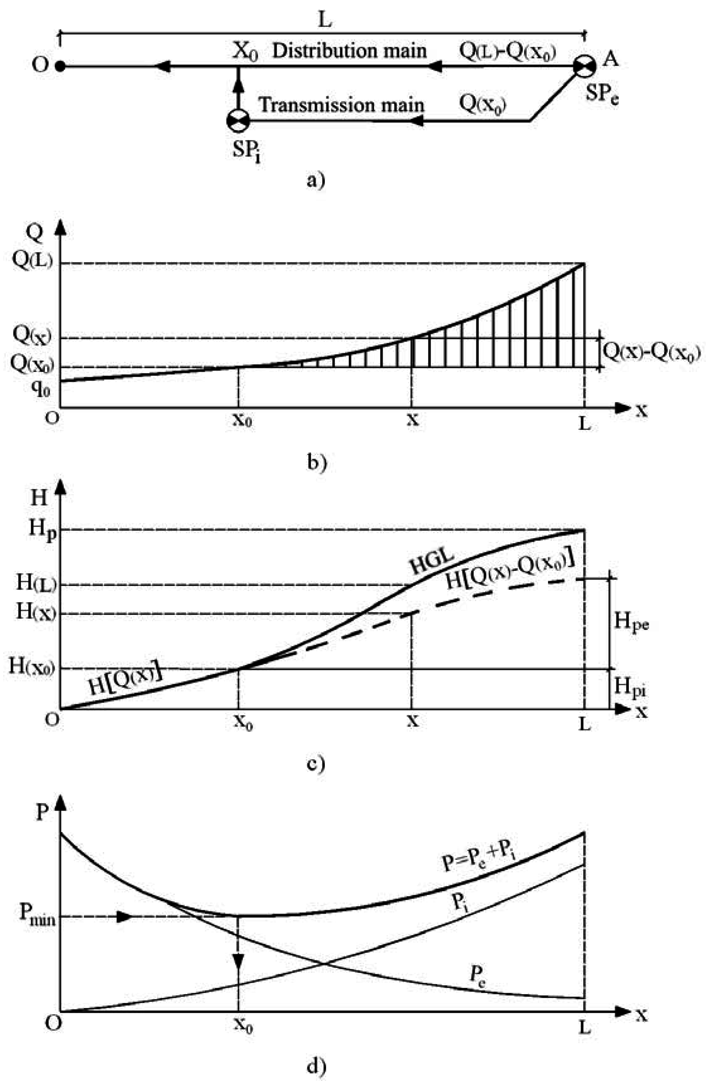
3.2. Intermediary Pumping Stations Integrated on the Distribution Mains
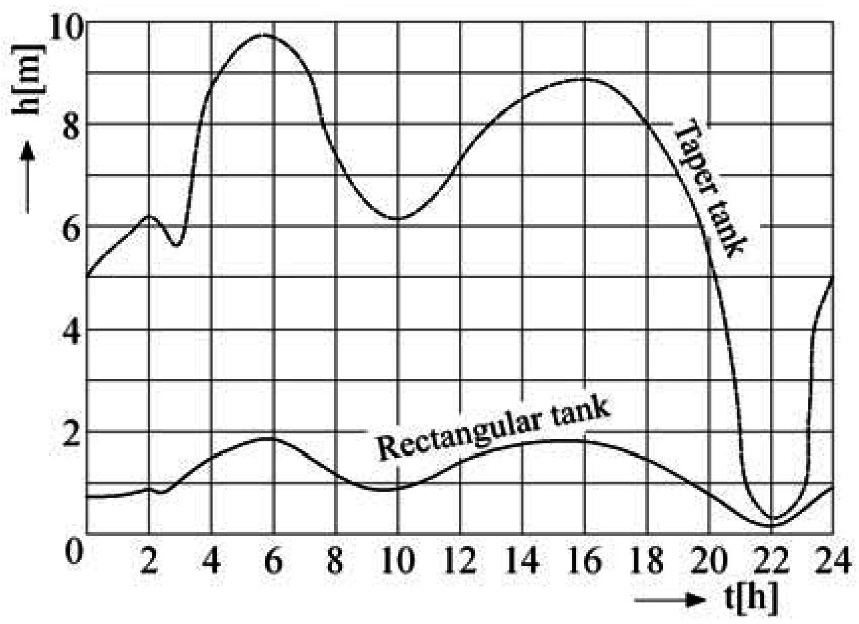
Direct integration of pumps on the network main pipes is a rational possibility for preservation of the energy used in the water distribution process.
On the distribution mains where a repumping station is mounted with parallel-connected pumps, water is taken over at a lower pressure p1 and repressed at a higher pressure p2, and the pump head is Hpi = (p2p1)/γ.
Use of serial-connected intermediary pump stations on some distribution mains amplifies the discharge through these pipes. These pump stations also generate a low pressure zone upstream in the suction node but ensures an important increase in pressure downstream in the pressure node. In this mode, favourable local increases in the piezometric head (HGL) in the system are generated. The repumping station is located almost at the suction node, and connection of the service lines at the upstream pipes is not made from the suction node but rather immediately downstream from the pump.
Considering that in a distribution system served by NP external pump stations (SPe) intermediary pump stations are directly serial-connected on a number of NA distribution mains, the total power in the system is:
P = γ η ( j = 1 N P Q p , j h p e , j + k = 1 N A Q p a , k H p i , k )
where Qp,j and hpe,j are the discharge and pump head, respectively, for external pump station j, and Qpak and Hpi,k are the discharge and pump head, respectively, for intermediary pump station k.
Because the pump heads of the external pump stations are decreased (hpe,j << Hpe,j) and the discharges of the intermediary pump stations became equal to the local discharges of the distribution mains on which they are integrated, a power reduction Δ P occurs according to Equation (9). As a result, electrical energy consumption in the system is reduced with Δ W.
The optimal solution for the location of the intermediary pump stations and the choice of their number, as well as the pumps from each of them, is determined by minimising the total installed power.

3.3. Elevated Tanks

A storage tank is considered to be “floating on the system” if the HGL in the tank is generally the same as the HGL in the system. Pumping into a system with an elevated storage tank (water tower) that floats on the system usually represents very efficient operation. Elevated tanks from water distribution networks present important level fluctuations via their compensatory function.
These tanks can be classified by shape as cylindrical, spherical, torroidal, taper, rectangular, and special [40]. The shape was optimised to make the technical and economic indicators as favourable as possible. For the optimal profile, due to the static and strength considerations, water surface elevation in a tank reaches higher values of 6–10 m, which increases the elevation of the HGL in the system and increases the pumping energy consumption.
The relatively higher cost of elevated tanks is justified by reducing the energy consumption during peak hours. At the peaks of the pumping schedule, when the electrical energy tariff is most expensive, it is recommended to deliver smaller discharges through the external pump stations and for the compensatory differences to be completed from the elevated tanks, which should be filled outside of these peak hours.
If the pumps are stopped during peak hours (approximately 4 h/day) and the urban centre is supplied from the volume accumulated in the elevated tanks during minimum consumption hours (when electricity tariff is small), an important reduction of the cost for electrical energy is achieved.
The consumed electrical energy W is evaluated as:
W = 9 . 81 η Q p H p e T p
where Qp is the pumped discharge in the system; Hpe is the maximum pump head (for a network supplied by one-sided pumping from the exterior); Tp is the pumping time; and η is the efficiency of the pump station.
The pump head is established as a function of the elevated tank location related to the pump station, the required pressure and the head losses in the transport pipes.
The cost economy obtained by the transfer of energy consumption from peak hours to base hours can be evaluated using the following equation:
C = 9 . 81 η Q p H p e T p ( e 1 e 2 )
where e1, and e2 are the estimated electric energy tariffs during peak hours and base hours, respectively.
Because of higher level oscillations, the advantages of peak energy savings could be lost by increasing global energy consumption. As a result, it is necessary to study the elevated tank behaviour in different constructive solutions and to study the way in which their potential characteristics influence the energy balance of the distribution.

3.4. Economic Indicators
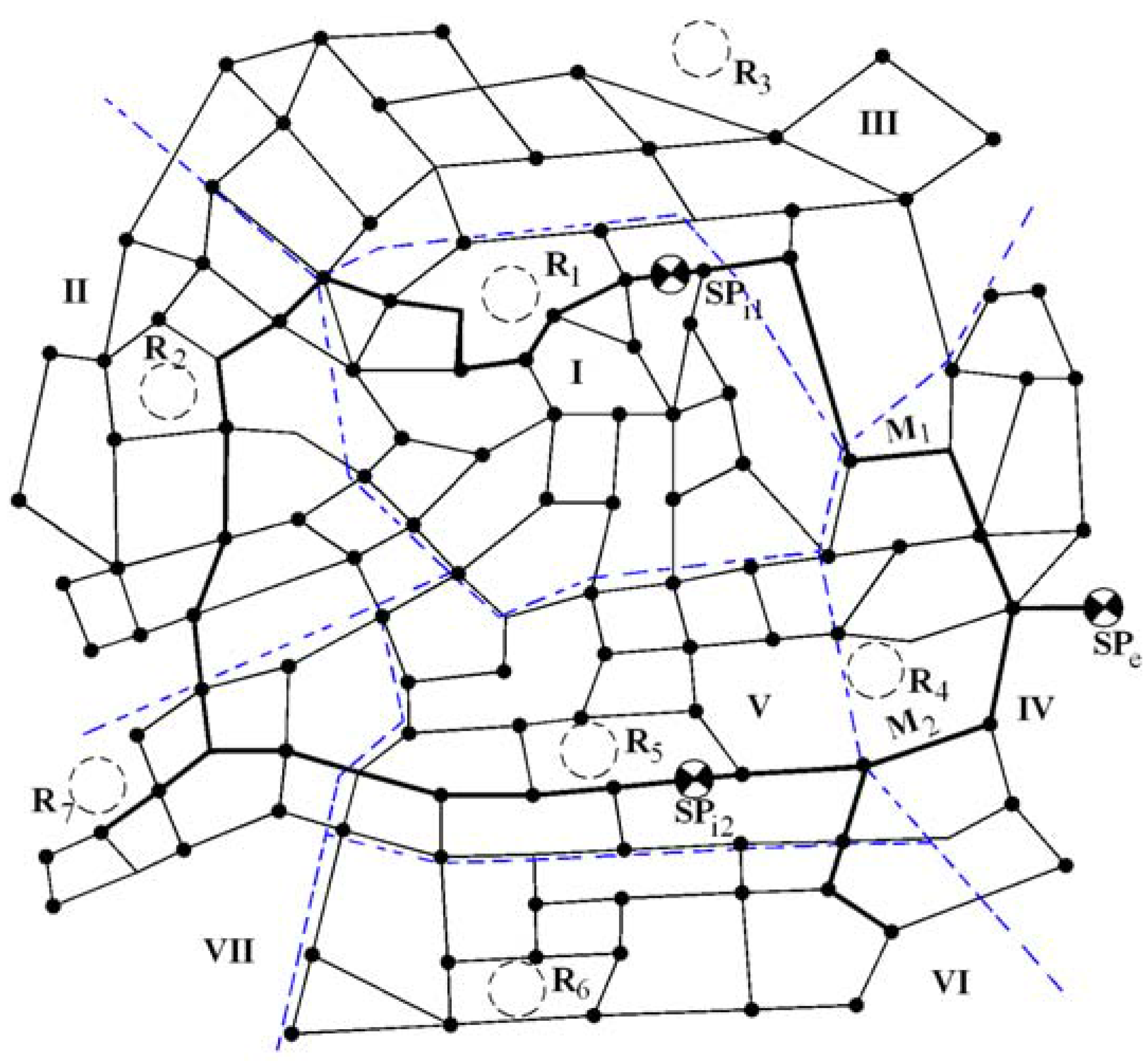
Incorporating potential elements into the water distribution system requires an additional investment, and its efficiency can be evaluated by the simply pay back time (SPBT), calculated as follows:
SPBT = Δ I C e C i < RT n
where Δ I is the additional investment for the optimised system; Ce is the annual operation cost for the reference system with the network supplied by one-sided pumping from the exterior; Ci is the annual operation cost for the system with internal potential elements; and RTn is the normal recovery time of 10–12 years.
Equation (17) can be reformulated in the following form [38]:
SPBT = Δ I Δ C w r Δ I < RT n
where Δ C w is the difference between the energy cost Cwe for the reference system and the energy cost Cwi for the optimised system and r is the repair, maintenance and periodic testing rate for the distribution system.

4. Case Studies

4.1. Potential Characteristics Influence of the Elevated Tanks on Distribution Energy Balance

Table 2 provides the hourly variations in water demand and pumped water during the day by relative amounts (the per cents αd and αp, and cumulative per cents Σαd and Σαp). Starting from this table, the compensatory function will be analysed for two types of elevated tanks: taper tank optimised, with generatrix angle of inclination 45° from the horizontal line, diameters of 36 m and 16 m, and maximum height of 10 m, and a rectangular (flat) tank with a height of 2 m. These water towers are located in the distribution system of a large urban centre from Romania and have an average hourly load equal to the maximum-day discharge Qdmax = 3.59 m3/s = 301,536 m3/day.
The hour-compensatory volume of an elevated tank is given by αv·Qdmax/100 and total compensatory capacity is defined as αvmax·Qdmax/100. The water height h was computed every hour for both types of tanks, as shown in Figure 6. On this basis, the comparative values of electricity consumption for both types of elevated tanks are reported in Table 3.

4.2. Energy–Economic Efficiency of Optimisation Solutions

A large urban industrial centre from Romania with the water distribution network illustrated in Figure 7 is considered. In this section, a comparative energy–economic analysis of the four optimisation solutions with internal potential elements proposed for water distribution is performed:
(1) First solution represents the classic reference case with an exterior pump station SPe at the water plant (direct pumping), which delivers a maximum-hour discharge Qhmax = 4.30 m3/s and an average pump head Hpe = 60 m. Taking into account the schedule of the hourly pumped discharge (Figure 8), the daily energy consumption W is determined.
(2) Second solution assumes partition of the town into seven distinct pressure zones, with a pumped storage tank located in each zone centre. The external pump station SPe supplies buried tanks Rk (k = 1 ... 7) of pumped storage through a low pressure looped transmission network (Figure 9). In this way, outside of the peak energy consumption hours, the maximum-day discharge Qdmax = 3.94 m3/s and the average pump head hpe = 15 m are continuously assured. The pumped storage pump stations generate via the buried tanks the hourly discharge Q, according to the pumping schedule from Figure 10, and the required pressure for the pressure zones.
The average pump heads corresponding to the pressure zones k have the following values, in m: 30.2, 40.8, 33.7, 43.6, 31.1, 37.5, and 29.6. The total daily energy consumption W for this solution is evaluated.
(3) Third solution replaces the buried tanks Rk with the elevated tanks Ck (k = 1 ... 7) with smaller levels of fluctuation, which ensures a gravitational distribution in the respective zones. The discharge Qdmax = 3.94 m3/s is pumped from external pump station SPe with an average pump head hpe = 49 m, according to the pumping schedule presented in Table 2, which sets a reduced pumping during peak hours of electricity consumption.
(4) Fourth solution consists of direct water pumping through intermediary pump stations SPi1 and SPi2 (Figure 7), assuming that the service pipes are connected immediately downstream of these stations. The intermediary pump stations are integrated on water mains M1 and M2. External pump station SPe delivers discharge Qhmax = 4.30 m3/s, with an average pumping head hpe = 40.5 m, and intermediary pump stations equipped with two sets of three parallel-connected pumps operating with discharges of 0.94 m3/s and 1.78 m3/s, for average pump heads Hpi,1 = 13.0 m and Hpi,2 = 11.4 m, respectively.
The supply network design of the buried tanks and the computation of the discharge and pressure distribution in the network for all of the analysed solutions were performed using computer programmes OPNELIRA [41] and ANOREC [35].

5. Results and Discussion

Table 3 provides the electricity consumption for water distribution using two types of elevated tanks. Because of the level of fluctuations and high water height, the case of the taper tank results in an energy consumption of 67,375 kWh/day compared with only 59,980 kWh/day in the case of a rectangular tank with a small water height.
In the second case, an energy savings of 2662 kWh/year was obtained, corresponding to a decrease in energy consumption of 11%.
Numerical results of the energy–economic efficiency for the four analysed solutions in Section 4.2 are reported in Table 4. The following parameters were set: r = 0.02, e1 = 0.23 €/kWh, e2 = 0.11 €/kWh.
In general, for urban industrial centres with other technological characteristics, the absolute values vary over a very large range, but the proportions at the level of comparable parameters are maintained and the results of comparative computations remain available.
The distribution system with zone pumped storage has an important advantage of reducing energy consumption by 5300 MWh/year, from which 4600 MWh/year occurs during peak hours, although the economic efficiency is near the limit (SPBT = 10 years) (Table 4).
Solution 4 of repumping with intermediary stations requires primarily small additional investments, but it ensures decreased energy consumption only under the assumption that service lines are supplied from the high pressure zone downstream of the integrated pump stations. If this condition is not realised due to constructive reasons, the HGL must be raised to 9 m to ensure the required pressure. As a result, the energy consumption increases, which reduces the energy efficiency of this solution, which is smaller than that of the solution with pumped storage tanks.
In this analysis, the optimal solution is considered to be Solution 2, with a convenient SPBT of 10 years and the greatest energy savings of 21% compared with the energy consumption in a reference unzoned distribution system.

6. Conclusions

Major findings of this study are concluded as follows:
Using potential elements can be replacing the doubling of distribution mains or increasing the diameters of the distribution mains, which are expensive solutions. In addition to the energy-efficient flow control in pumping, the rotational speed control using VSDs for each parallel-connected pump can open new opportunities for the advanced control of the pumping processes.
This study confirmed the favourable energy–economic efficiency for the procedure of determining the optimal location of pumped storage supply via low pressure transmission mains and the use of buried tanks and internal pump stations. This procedure leads to energy savings of 8%–21% and provides the possibility of chlorine step dosage for water disinfection, enabling a smaller dose of chlorine at the water plant tanks.
The case of distribution networks with elevated tanks usually does not result in an absolute reduction of electricity, but, generally, the energy cost is diminished because of the scheduling of the more intense pumping outside of the peak hours of energy consumption. The absolute decrease in energy consumption in the case of elevated rectangular tanks of low water height demands these structures in a water distribution system.
The use of intermediary pump stations integrated on distribution mains has the advantages of making the pressure more uniform in large networks, avoiding the zones with exaggerated high pressure. However, some low pressure zones appear at the initial node of the distribution main on which the repumping station is located. This deficiency can be completely eliminated by connecting the service lines upstream of a pump.
Because water supply systems are executed sequentially, the proposed solutions for energy optimisation of the water distribution can be combined while respecting the essential principles in the structural development of the system.

Conflicts of Interest
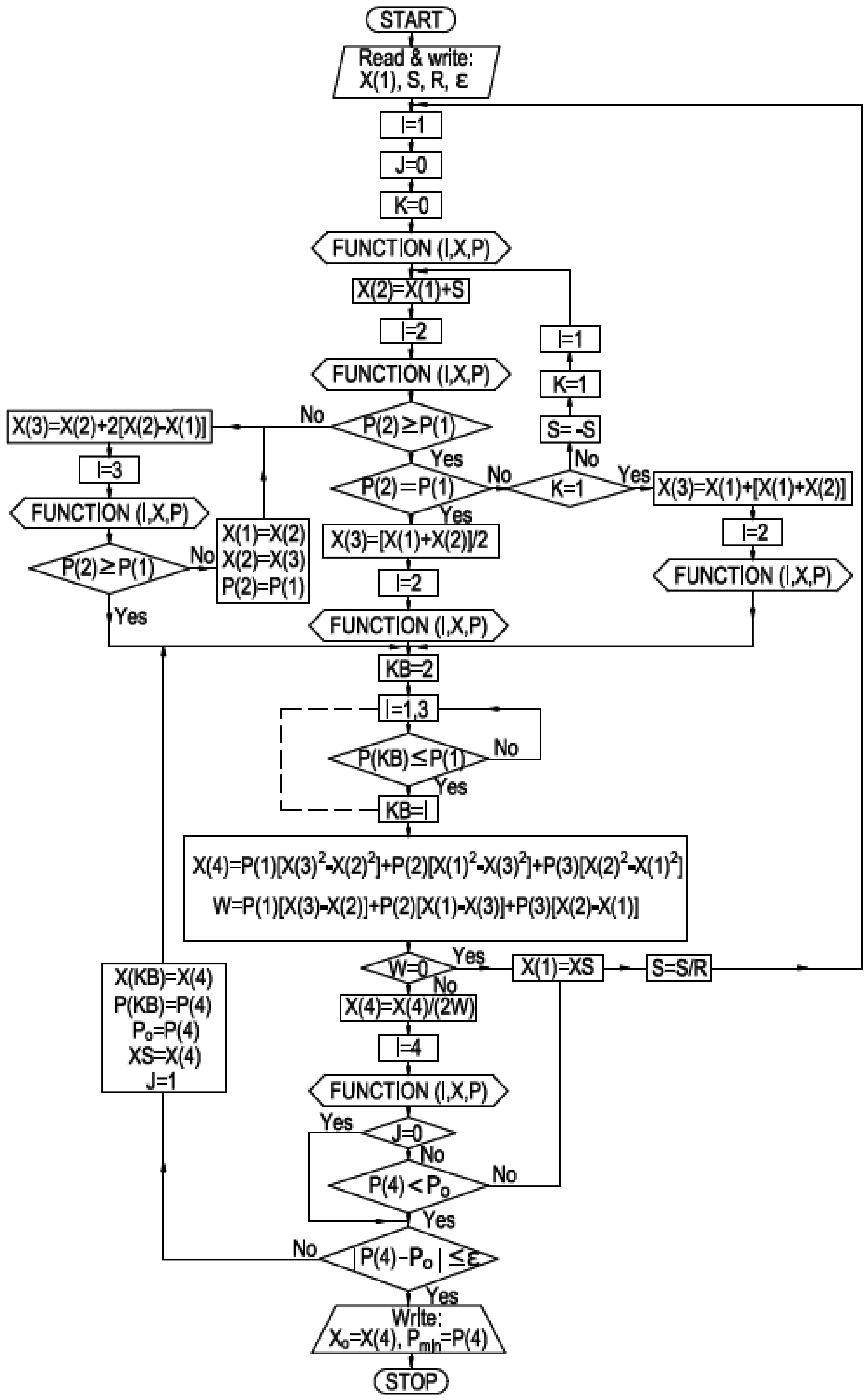
The author declares no conflict of interest.

Appendix A

Substituting Equations (11) and (12) into Equation (10) and integrating, the resulting equation until section X0 is obtained:
H ( x 0 ) = r 0 q 0 β x 0 b q 0 β 3 x 0 3 + r 0 a β β α + 1 x 0 β α + 1 b a β β α + 3 x 0 β α + 3
To describe the hydraulic regime upstream of section X0, the discharge equation can be written under a simple form:
Q ( x ) = Q ( x ) Q ( x 0 ) = a ( x α x 0 α )
This equation results in the piezometric head (HGL) in the supply node of the distribution main:
H ( L ) = H ( x 0 ) + r 0 a β β α + 1 L β α + 1 b a β β α + 3 L β α + 3 r 0 a β β α + 1 x 0 β α + 1 + b a β β α + 3 x 0 β α + 3
and the expressions of the pump stations’ power:
P i = γ η Q ( x 0 ) H ( x 0 )
P e = γ η [ Q ( L ) Q ( x 0 ) ] [ H ( L ) H ( x 0 ) ]
Taking into account Equations (A4) and (A5), the total power P = Pe + Pi can be expressed as:
P = γ η { [ Q ( L ) Q ( x 0 ) ] [ H ( L ) H ( x 0 ) ] + Q ( x 0 ) H ( x 0 ) }

References

  1. Watergy. 2009. Available online: http://www.watergy.net/-overview/why.php (accessed on 5 June 2015).
  2. Moreira, D.F.; Ramos, H.M. Energy cost optimization in a water supply system case study. J. Energy 2013. [Google Scholar] [CrossRef]
  3. Coelho, B.; Andrade-Campos, A. Efficiency achievement in water supply systems–A review. Renew. Sustain. Energy Rev. 2014, 30, 59–84. [Google Scholar] [CrossRef]
  4. Bene, J.G.; Selek, I.; Hös, C. Neutral search technique for short-term pump schedule optimization. J. Water Resour. Plan. Manag. 2010, 136, 133–137. [Google Scholar] [CrossRef]
  5. Vilanova, M.R.N.; Balestieri, J.A.P. Energy and hydraulic efficiency in conventional water supply systems. Renew. Sustain. Energy Rev. 2014, 30, 701–7014. [Google Scholar] [CrossRef]
  6. Walski, T.M.; Chase, D.V.; Savic, D.A.; Grayman, W.; Beckwith, S.; Koelle, E. Advanced Water Distribution Modeling and Management; Haestad Press: Waterbury, CT, USA, 2003. [Google Scholar]
  7. Binder, A. Potentials for energy saving with modern drive technology: A survey. In Proceedings of the International Symposium on Power Electronics, Electrical Drives, Automation and Motion, Ischia, Italy, 11–13 June 2008.
  8. Pemberton, M.; Bachmann, J. Pump systems performance impacts multiple bottom lines. Eng. Min. J. 2010, 211, 56–59. [Google Scholar]
  9. Ferreira, F.J.T.E.; Fong, C.; de Almeida, T. Eco-analysis of variable-speed drives for flow regulation in pumping system. IEEE Trans. Ind. Electron. 2011, 58, 2117–2125. [Google Scholar] [CrossRef]
  10. Zhang, H.; Xia, X.; Zhang, J. Optimal sizing and operation of pumping systems to achieve energy efficiency and load shifting. Electr. Power Syst. Res. 2012, 86, 41–50. [Google Scholar] [CrossRef]
  11. McCormick, G.; Powell, R.S. Optimal pump scheduling in water supply systems with maximum demand charges. J. Water Resour. Plan. Manag. 2003, 129, 372–379. [Google Scholar] [CrossRef]
  12. Van Zyl, J.E.; Savic, D.A.; Walters, G.A. Operational optimization of water distribution systems using a hybrid genetic algorithm. J. Water Resour. Plan. Manag. 2004, 130, 160–170. [Google Scholar] [CrossRef]
  13. Salomons, E.; Goryashko, A.; Shamir, U.; Rao, Z.; Alvisi, S. Optimizing the operation of the Haifa: A water distribution network. J. Hydroinf. 2007, 9, 51–64. [Google Scholar] [CrossRef]
  14. Lopez-Ibáñez, M.; Prasad, T.D.; Paechter, B. Ant colony optimization for optimal control of pumps in water distribution networks. J. Water Resour. Plan. Manag. 2008, 134, 337–346. [Google Scholar] [CrossRef]
  15. Broad, D.R.; Maier, H.R.; Dandy, G.C. Optimal operation of complex water distribution systems using metamodels. J. Water Resour. Plan. 2010, 136, 433–443. [Google Scholar] [CrossRef]
  16. Vogelesang, H. Two approaches to capacity control. World Pumps 2009, 511, 26–29. [Google Scholar] [CrossRef]
  17. Pemberton, M. Intelligent variable speed pumping. Plant Eng. 2003, 57, 28–30. [Google Scholar]
  18. Bortoni, E.; Almeida, R.A.; Viana, A.N.C. Optimization of parallel variable-speed-driven centrifugal pumps operation. Energy Effic. 2008, 1, 167–173. [Google Scholar] [CrossRef]
  19. Yang, Z.; Borsting, H. Energy efficient control of a boosting system with multiple variable-speed pumps in parallel. In Proceedings of the 49th IEEE Conference on Decision and Control, Atlanta, GA, USA, 15–17 December 2010.
  20. Viholainen, J.; Tamminen, J.; Abhonen, T.; Ahola, J.; Vakkilainen, E.; Soukka, R. Energy-efficient control strategy for variable speed-driven parallel pumping systems. Energy Effic. 2013, 6, 495–509. [Google Scholar] [CrossRef]
  21. Araujo, L.S.; Ramos, H.; Coelho, S.T. Pressure control for leakage minimisation in water distribution systems management. Water Resour. Manag. 2006, 20, 133–149. [Google Scholar] [CrossRef]
  22. Carravetta, A.; Del Giudice, G.; Fecarotta, O.; Ramos, H.M. Energy production in water distribution networks: A PAT design strategy. Water Resour. Manag. 2012, 26, 3947–3959. [Google Scholar] [CrossRef]
  23. Diniz, A.M.F.; Fontes, C.H.; da Costa, C.A.; Costa, G.M.N. Dynamic modeling and simulation of water supply system with applications for improving energy efficiency. Energy. Effic. 2014, 8, 417–432. [Google Scholar] [CrossRef]
  24. Nazif, S.; Karanouz, M.; Moridi, A. Pressure management model for urban water distribution networks. Water Resour. Manag. 2010, 24, 437–458. [Google Scholar] [CrossRef]
  25. Lenzi, C.; Bragalli, C.; Bolognesi, A.; Artina, S. From energy balance to energy efficiency indicators including water losses. Water Sci. Technol. Water Supply 2013, 13, 889–895. [Google Scholar] [CrossRef]
  26. Sarbu, I.; Ostafe, G. Energetically optimization of water distribution systems in large urban centers. Period. Polytech. Mech. Eng. 2008, 52, 93–102. [Google Scholar] [CrossRef]
  27. Feldman, M. Aspects of energy efficiency in water supply systems. In Proceedings of the 5th IWA Water Loss Reduction Specialist Conference, Cape Town, South Africa, 26–30 April 2009.
  28. Rishel, J.B. Water Pumps and Pumping Systems; McGraw-Hill: New York, NY, USA, 2002. [Google Scholar]
  29. Marchi, A.; Simpson, A.R.; Ertugrul, N. Assessing variable speed pump efficiency in water distribution systems. Drink. Water Eng. Sci. 2012, 5, 15–21. [Google Scholar] [CrossRef]
  30. Sarbu, I.; Borza, I. Energetic optimization of water pumping in distribution systems. Period. Polytech. Mech. Eng. 1998, 42, 141–152. [Google Scholar]
  31. Hooper, W. Advantages of parallel pumping. Plant Eng. 1999, 31, 4–6. [Google Scholar]
  32. Volk, M. Pump Characteristics and Applications; Taylor & Francis Group: Boca Raton, FL, USA, 2005. [Google Scholar]
  33. Kaya, D.; Yagmur, E.A.; Yigit, K.S.; Kilic, F.C.; Eren, A.S.; Celik, C. Energy efficiency in pumps. Energy Convers. Manag. 2008, 49, 1662–1673. [Google Scholar] [CrossRef]
  34. Gibson, I.H. Variable-speed dives as flow control elements. ISA Trans. 1994, 33, 165–169. [Google Scholar] [CrossRef]
  35. Sarbu, I. Nodal analysis of urban water distribution networks. Water Resour. Manag. 2014, 28, 3143–3159. [Google Scholar] [CrossRef]
  36. Sarbu, I. Analysis of looped water supply networks. La Houille Blanche 2001, 3–4, 138–142. [Google Scholar]
  37. Démidovitch, B.; Maron, I. Elements de Calcul Numerique; Mir: Moscou, Russia, 1979. [Google Scholar]
  38. Sarbu, I. Energy Optimization of Water Distribution Systems; Romanian Academy Publishing House: Bucharest, Romania, 1997. [Google Scholar]
  39. Polak, E. Computational Methods in Optimization; Academic Press: New York, NY, USA, 1971. [Google Scholar]
  40. Walski, T.M. Hydraulic design of water distribution storage tanks. In Water Distribution System Handbook; McGraw Hill: New York, NY, USA, 2000. [Google Scholar]
  41. Sarbu, I.; Kalmar, F. Optimization of looped water supply networks. Period. Polytech. Mech. Eng. 2002, 46, 75–90. [Google Scholar]
Figure 1. Flow rate adjustment using pump speed control.
Water 08 00593 g001
Figure 2. Variation of the centrifugal pump curves.
Water 08 00593 g002
Figure 3. Characteristic curves H-Q, η-Q and the operating points for different parallel-connected pumps.
Water 08 00593 g003
Figure 4. Optimal location of a pumped storage tank. (a) Schematic of the distribution main; (b) Discharge distribution; (c) Head loss variation; (d) Power variation of the external and internal pump stations.
Water 08 00593 g004
Figure 5. Flow chart of searching algorithm with an accelerated step.
Water 08 00593 g005
Figure 6. Water level fluctuation in elevated tanks.
Water 08 00593 g006
Figure 7. Schematic of the analysed distribution network.
Water 08 00593 g007
Figure 8. Pumping schedule of SPe for the reference solution.
Water 08 00593 g008
Figure 9. Schematic of the supply network of pumped storage tanks.
Water 08 00593 g009
Figure 10. Pumping schedule for pumped storage tanks.
Water 08 00593 g010
Table 1. The specific energy consumption and energy savings obtained with control methods.
Adjustment MethodPeriod (h)Number of Operating PumpsPumped Flow Q (m3/s)Pump Head Hp (m)Absorbed Power P (kW)Consumed Energy W (kWh/Day)Specific Energy Consumption w (%)
1. Classical (start–stop)0:00–4:003 pf1.4738.6696.331,705.6100
4:00–10:006 pf2.4849.81730.8
10:00–14:004 pf1.9142.5995.4
14:00–17:005 pf2.1845.71303.1
17:00–22:006 pf2.4849.81730.8
22:00–24:004 pf1.9142.5995.4
2. Throttle valve control0:00–5:003 pf1.4738.6696.327,970.588
5:00–6:006 pf2.2553.01424.0
6:00–7:006 pf2.4849.81730.8
7:00–8:006 pf2.2553.01424.0
8:00–10:005 pf2.0847.51138.2
10:00–12:004 pf1.9142.5995.4
12:00–13:005 pf1.8156.01181.6
13:00–15:004 pf1.9142.5995.4
15:00–16:006 pf2.0847.51138.2
16:00–20:006 pf2.2553.01424.0
20:00–23:006 pf2.4650.01544.1
23:00–24:004 pf1.8143.01122.6
3. Rotational speed control0:00–5:002pf + 1pv1.4237.6655.225,375.580
5:00–6:005pf + 1pv2.2545.51222.5
6:00–7:006 pf2.4849.81730.8
7:00–8:005pf + 1pv2.2545.51222.5
8:00–10:005 pf2.0843.01030.3
10:00–12:004 pf1.9142.5995.4
12:00–1:003pf + 1pv1.8140.0708.9
13:00–15:004 pf1.9142.5995.4
15:00–16:005pf2.0843.01030.3
16:00–20:005pf + 1pv2.2545.51222.5
20:00–23:005pf + 1pv2.4649.61534.5
23:00–24:003pf + 1pv1.8140.0708.9
Energy saving, ΔW2-1(MWh/year)1345.0
(%)11.6
Energy saving, ΔW3-1(MWh/year)2280.0
(%)20
Energy saving, ΔW3-2(MWh/year)935.0
(%)8.4
Table 2. Estimation of elevated tanks capacity for hour demand compensation.
Period (h)Demand Percentage, (%)Pumping Percentage, (%)Compensation Percentage, (%)Compensatory Volume, (%)
αdΣαdαpΣαpαc = αp − αdΣαcαv
0:00–1:003.303.304.504.501.201.202.80
1:00–2:003.256.554.509.001.252.454.05
2:00–3:003.259.804.5013.501.253.705.30
3:00–4:003.2513.054.5018.001.254.956.55
4:00–5:003.4016.454.5022.501.106.057.65
5:00–6:003.9520.404.5027.000.556.60 (max)8.20 (max)
6:00–7:004.8025.204.5031.50−0.306.307.90
7:00–8:005.2530.402.5034.00−2.703.605.20
8:00–9:004.5534.953.0037.00−1.552.053.65
9:00–10:004.5539.504.5040.50−0.052.003.60
10:00–11:004.6044.105.5047.000.902.904.50
11:00–12:004.5048.605.2052.501.003.905.50
12:00–13:004.7553.355.2557.750.504.406.00
13:00–14:004.5057.855.2563.000.755.156.75
14:00–15:004.3062.155.0068.000.705.857.45
15:00–16:004.2566.404.5072.500.256.107.70
16:00–17:004.2070.604.2576.750.056.157.75
17:00–18:004.1074.702.5079.25−1.604.556.15
18:00–19:004.2078.902.5081.75−1.702.854.45
19:00–20:004.3083.102.8584.60−1.451.403.00
20:00–21:005.0088.203.0087.75−2.00−0.451.15
21:00–22:004.8093.003.6591.40−1.15−1.60 (min)0.00
22:00–23:003.6096.604.2595.500.65−1.100.50
23:00–24:003.40100.004.50100.001.100.001.60
Table 3. Computation of energy consumption for water distribution using elevated tanks.
Period (h)PumpingTaper TankRectangular Tank
αp (%)Qp (m3/s)Hp (m)P (kW)W (kWh/Day)Hp (m)P (kW)W (kWh/Day)
0:00–1:004.504.2553.6298067,375.043.7271059,980.0
1:00–2:004.504.2554.4302548.82715
2:00–3:004.504.2553.6298048.72710
3:00–4:004.504.2556.8316049.02725
4:00–5:004.504.2557.2318049.52750
5:00–6:004.504.2557.7320549.82770
6:00–7:004.504.2556.8315549.82770
7:00–8:002.502.3656.4174049.31520
8:00–9:003.002.8356.3208548.91810
9:00–10:004.504.2554.0300048.82710
10:00–11:005.505.2054.5370549.03330
11:00–12:005.204.9155.7358049.23160
12:00–13:005.254.9656.2364549.33200
13:00–14:005.254.9656.7368049.43205
14:00–15:005.004.7356.8351549.53060
15:00–16:004.504.2556.9316049.92775
16:00–17:004.254.0256.8298549.72615
17:00–18:002.502.3656.5174549.61530
18:00–19:002.502.3655.3170549.31520
19:00–20:002.852.0354.2144048.91300
20:00–21:003.002.8353.8199048.41790
21:00–22:003.503.3049.4213048.12075
22:00–23:004.254.0250.4265048.12530
23:00–24:004.504.2552.8293546.82700
Energy saving, ΔW(MWh/year)2662
(%)11
Table 4. Energy–economic indicators of analysed solutions.
No.IndicatorSolution
(1)(2)(3)(4)
1Additional investment, 10−3ΔI [€]
– transmissions mains12401240
– tanks157625
– pump stations5263
Total1449186563
2Average pump head, Hp [m]
– external pump station60154940.5
– internal pump stations3512
3Consumed energy, W [MWh/year]
– external pump station25,300660021,60019,600
– internal pump stations13,4003600
Total25,30020,00021,60023,200
Peak7300270034005400
4Operation cost, 10−3Cw [€/year]
–energy cost difference, 10−3ΔCw17013567
–pay-off rate, 10−3rΔI29381
Costs difference, 10−3CwpΔI)1419766
5SPBT [years]10191
6Energy saving, ΔW(MWh/year)530037002100
(%)21158

