Risk Analysis of Reservoir Flood Routing Calculation Based on Inflow Forecast Uncertainty

Abstract

Possible risks in reservoir flood control and regulation cannot be objectively assessed by deterministic flood forecasts, resulting in the probability of reservoir failure. We demonstrated a risk analysis of reservoir flood routing calculation accounting for inflow forecast uncertainty in a sub-basin of Huaihe River, China. The Xinanjiang model was used to provide deterministic flood forecasts, and was combined with the Hydrologic Uncertainty Processor (HUP) to quantify reservoir inflow uncertainty in the probability density function (PDF) form. Furthermore, the PDFs of reservoir water level (RWL) and the risk rate of RWL exceeding a defined safety control level could be obtained. Results suggested that the median forecast (50th percentiles) of HUP showed better agreement with observed inflows than the Xinanjiang model did in terms of the performance measures of flood process, peak, and volume. In addition, most observations (77.2%) were bracketed by the uncertainty band of 90% confidence interval, with some small exceptions of high flows. Results proved that this framework of risk analysis could provide not only the deterministic forecasts of inflow and RWL, but also the fundamental uncertainty information (e.g., 90% confidence band) for the reservoir flood routing calculation.

1. Introduction

Flood forecasting is an important component of nonstructural measures of flood control and disaster reduction. However, the deterministic forecasts (always with biases) cannot provide objective assessment of possible risks in the flood control measures and decision-making scheduling scheme [1,2]. Due to the complexity of natural hydrological processes and the limitations of human understanding, there are inevitably many uncertainties in flood forecasting; for example, input, model structure, and parameter uncertainties may exist when using hydrological models [3,4,5,6]. Many researchers have conducted numerous valuable studies on hydrologic uncertainty analysis and probabilistic flood forecasting (PFF); e.g., [7,8,9,10,11,12]. According to these pioneer studies, three main benefits of PFF can be summarized as follows: (1) directly outputs the confidence intervals that describe total uncertainties in operational forecasts; (2) supports the flood warning and emergency response system through the set of risk indicators; and (3) helps the decision-makers conduct the flood control and scheduling based on the risk theory. In most PFF studies, the input conditions, parameters, and model settings of hydrologic models are viewed as random variables, following certain probability distributions, and thus model output could also be described with a certain probability distribution. Such model outputs can provide not only the mean forecasts, but also the probability estimates and confidence levels of forecasts at each time step for flood control and scheduling [13].

Reservoir flood control and scheduling decision-making is a difficult and systematic task, involving flood control standard requirements in the upstream and downstream, and the trade-off between flood control and refill. This complexity inevitably leads to uncertainties or risks in decision-making. Thus, risk analysis in both flood routing and scheduling has been one of the hot topics in the operation and management of reservoirs for a long time [14,15,16]. The uncertainty of flood routing is one of the main sources of forthcoming risk. Traditionally, reservoir flood control and scheduling analysis is the determination of reasonable gate operation and regulation based on the dynamic relationship between reservoir level and discharge volume. Therefore, uncertainties in the flood routing calculation may result in unpredictable risks of dam failing. With socio-economic development, dam failure losses become greater and unacceptable [17]. Thus, the risk analysis of reservoir flood routing calculations should be fully appreciated in order to understand and reduce the risks.

The present paper describes a framework for the risk analysis calculation of reservoir flood routing, considering the inflow forecast uncertainty (with hydrologic models), and further demonstrates a case study of the Meishan Reservoir in the Huaihe River, China. Inflow forecast uncertainty was analyzed through the integration of the Xinanjiang hydrologic model [18,19,20] and the Hydrologic Uncertainty Processor (HUP), which is a sub-model of the Bayesian Forecasting System (BFS) [8]. It is noted that risk usually includes both exposure loss and the possibility of loss, but as an example, only the possibility of loss (reservoir water level exceeding a defined safety control level) was studied in this paper.

2. Materials and Methods

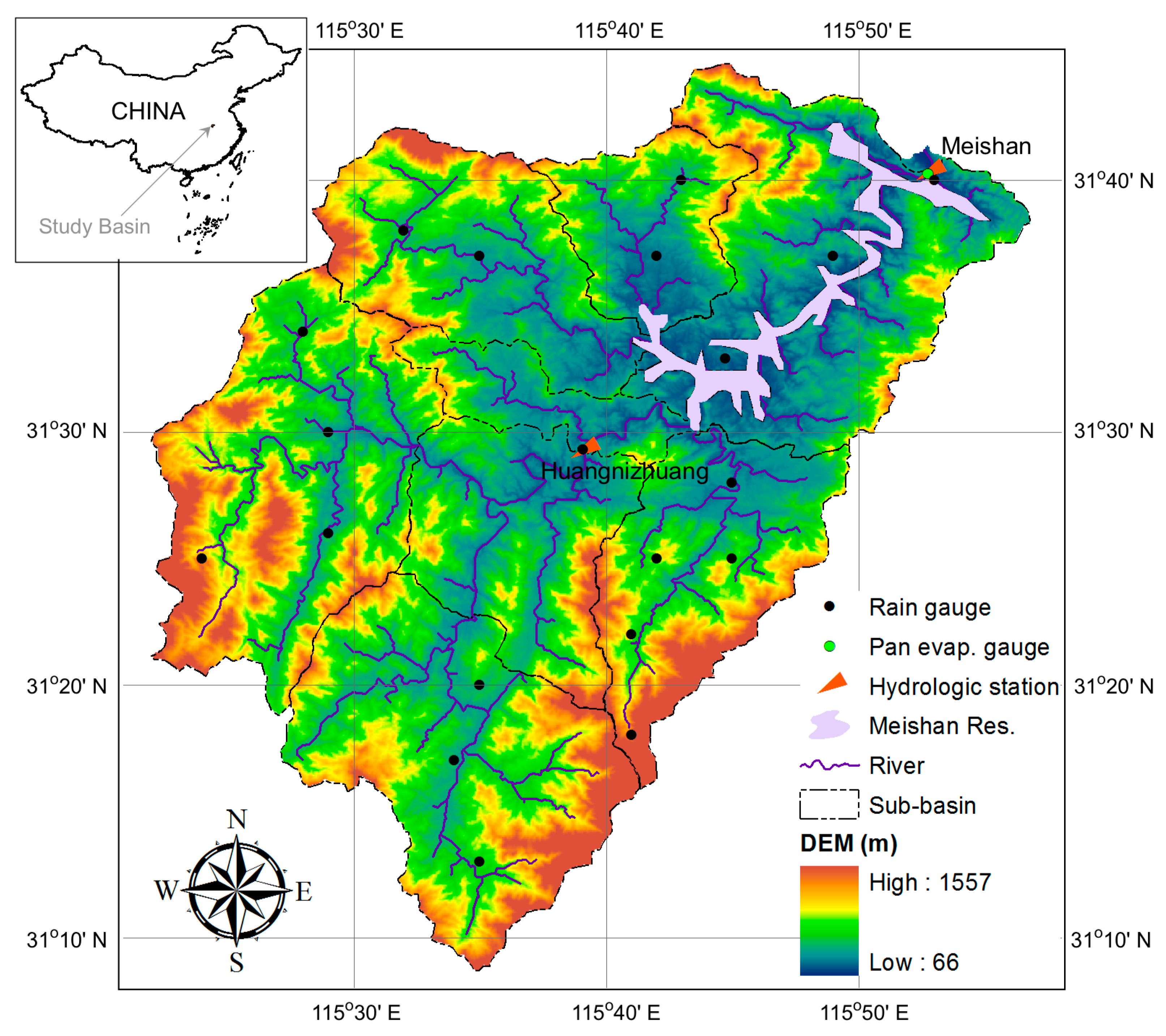
2.1. Study Basin and Forcing Data

The Meishan Reservoir, built in 1958, is located at the upstream of Shihe River, which is a tributary of Huaihe River, East China (Figure 1). The drainage basin subtended by this reservoir (denoted hereafter as Meishan basin) covers an area of 1970 km², with a river length of about 86 km. Mountain and hill are two main landforms, and the topography decreases from south to north in the basin. The upstream mountainous area is characterized by steep slope, rapid-flow, and high forest coverage, while most area in the downstream basin is also covered by vegetation. The study area is dominated by the northern subtropics monsoon climate, with mean annual precipitation of about 1400 mm, but up to 60% of the precipitation occurs during the period of June–September. In the basin, the dominating runoff mechanism is saturation excess (Dunne) runoff.

According to both requirements of flood control and benefits promotion, the current reservoir regulation rules for the main flood season are as follows [21]: (1) reservoir tunnels should be opened for flood releasing when the reservoir water level (RWL) is greater than the flood limit water level (FLWL, 125.27 m), but the discharge rate should not be greater than 1200 m³/s if RWL < 130.07 m; (2) the discharge rate should be increased gradually when RWL > 130.07 m; and (3) all tunnels and spillways should be opened to maximize the discharge rate when RWL > 133 m. The relationship between RWL, reservoir water volume (RWV), and discharge rate is shown in Figure 2. In addition, the characteristic water levels for the Meishan Reservoir are also available [20]: dead water level = 107.07 m, normal water level = 126 m, top level of flood control = 133 m, design flood level = 139.17, and check flood level = 140.77 m.

In total, there are 20 rain gauges, two hydrologic stations, and one pan evaporation gauge (E601) distributed in the Meishan basin (Figure 1). Observed daily data of rainfall, pan evaporation, and discharge for the period of 1980–2010, and hourly rainfall and discharge data for some flood events in the rainy season from April to October were collected for the analysis. It should be noted that the observed reservoir inflow data (provided by the local Reservoir Management Department) were calculated according to the reservoir water volume/level data at Meishan station with an inverse method. Floods with different magnitudes, including low, median, and high flows were selected. The areal mean values of rainfall and evaporation were calculated with the Thiessen polygon interpolation, which may be of excessive geometrical features in polygon boundaries. However, the limitation of this technique would be weakened in the sub-basin scale only when areal mean variables were used.

2.2. The Xinanjiang Model

The Xinanjiang model has been widely studied and applied to flood forecasts in (semi-) humid regions of China since developed in early 1970s [18,19,20]. The saturation excess mechanism was assumed for runoff formation. A parabola-type cumulative distribution function (CDF) is used to represent the spatial variation of soil tension water capacity over the basin. Similar CDFs were employed in other models, such as the Variable Infiltration Capacity (VIC) model [22], the ARNO model [23], and the Statistical Runoff Model [24]. The formula of the soil tension water capacity curve can be expressed as:

$$\mathsf{\alpha }=1-{\left(\frac{W_m^{\text{'}}}{W_{mm}^{\text{'}}}\right)}^B,W_{mm}^{\text{'}}=\frac{1+B}{1-IM}WM,$$

(1)

where $W_m^{\text{'}}$ is the tension water capacity at a point that varies from zero to a maximum $W_{mm}^{\text{'}}$; α represents the proportion of the pervious area of the basin whose tension water capacity is less than or equal to a specific value of $W_m^{\text{'}}$; WM is the areal mean tension water capacity; IM is the impervious area ratio of the basin, and B is a parameter. In the calculation of runoff generation, the areal mean initial tension water storage over the basin is defined as W, whose maximum at a point is A:

$$A=W_{mm}^{\text{'}}\left[1-{\left(1-\frac{W}{WM}\right)}^{\frac{1}{1+B}}\right].$$

(2)

Total runoff can be calculated according to the soil moisture condition of the basin that is fully saturated or not:

$$\{\begin{array}{l}\begin{array}{cc}R=P-E+W-WM+WM{\left(1-\frac{P-E+A}{W_{mm}^{\text{'}}}\right)}^{B+1},& A+P-E\le W_{mm}^{\text{'}}\end{array}\\ \begin{array}{cc}R=P-E+W-WM,& A+P-E\ge W_{mm}^{\text{'}}\end{array}\end{array},$$

(3)

where R is the total runoff; P is the areal mean rainfall; and the areal mean actual evaporation (E) can be estimated from potential evapotranspiration (E_P = KC·E₀) based on a three-layer soil moisture model, where E₀ is pan evaporation and KC is a ratio.

• when WU + P ≥ E_P,

  EU = E_P, EL = 0, ED = 0;

  (4)
• when WU + P < E_P and WL ≥ C·WLM,

  EU = WU + P, EL = (E_P − EU)·WL/WLM, ED = 0;

  (5)
• when WU + P < E_P and C·(EP − EU) ≤ WL < C·WLM,

  EU = WU + P, EL = C·(E_P − EU), ED = 0;

  (6)
• when WU + P < E_P and WL < C·(EP − EU),

  EU = WU + P, EL = WL, ED = C·(E_P − EU) − EL;

  (7)

where EU, EL, and ED are the actual evaporation from the upper, lower, and deep layers, respectively (E = EU + EL + ED); WU, WL, and WD are the areal mean tension water storage of these three layers, and their corresponding capacity are denoted as WUM, WLM, and WDM (WM = WUM + WLM + WDM); C is a parameter.

Total runoff was separated into surface, interflow, and groundwater components, and concentrated to the outflow of each sub-basin by a lag and route method by eight parameters: SM = areal mean free water storage capacity (mm); EX = a parameter in the distribution of free water storage capacity; KG = a coefficient for calculating the outflow to groundwater storage; KI = a coefficient for calculating the outflow to interflow storage; CI = interflow reservoir constant of the sub-basin; CG = groundwater reservoir constant of the sub-basin; CS = the “route” parameter of the flow concentration within the sub-basin; L = the “lag” parameter of the flow concentration within the sub-basin (hours). The channel routing calculation of rivers connecting the sub-basins was conducted by the Muskingum routing method. In total, there are 15 parameters for runoff production in the Xinanjiang model, and the detailed description of the model can be found in [18,19].

In this study, the Xinanjiang model was running in a semi-distributed mode with the meteorological input of rainfall and pan evaporation. The Meishan basin was divided into eight sub-basins, while three of them are located in the drainage area above the Huangnizhuang station (Figure 1). Following the usual practices in the hydrology community, the flood events were selected for calibration and validation purposes according to the time sequence, and a larger number of floods were used for model calibration than for validation. Both calibration and validation included different magnitudes of floods in order to determine the optimized parameters. We collected more observed flow data at the Huangnizhuang station than the Meishan station. Thus, the Xinanjiang model was calibrated with 15 flood events at the Huangnizhuang station and further validated with forcing data of both Huangnizhuang and Meishan station (five and ten flood events, respectively) at hourly time steps. The initial condition (soil moisture) of each flood event was simulated by continuously running the Xinanjiang model at daily time steps.

2.3. The HUP Model

The HUP is a component of the BFS, and its task is to quantify the hydrologic uncertainty under the hypothesis that there is no precipitation uncertainty [25]. In the HUP model, the Bayesian theory is used to express the posterior density function of observed flow, and Meta-Gaussian function sets are used to simplify the calculation process of this function. Suppose H₀ is the given observed flow when it is forecasted; the variables H_n and S_n (n = 1, 2,…, N) are the actual flow process and the forecasted flow process of deterministic hydrologic model, respectively; and N is the lead time. The specific values h_n and s_n are used instead of the observed value H_n and the estimated value S_n, respectively. Based on the Bayesian theorem, when S_n = s_n, for any time n and observations H₀ = h₀, the posterior density function of H_n is as [26]:

$${\Phi }_n\left(h_n|s_n,h_0\right)=\frac{f_n\left(s_n|h_n,h_0\right)g_n\left(h_n|h_0\right)}{{\displaystyle {\int }_{-\infty }^{\infty }{f}_n\left(s_n|h_n,h_0\right)g_n\left(h_n|h_0\right)d{h}_n}},$$

(8)

where the prior density function g_n takes the natural uncertainty of hydrologic elements into consideration; the likelihood function f_n describes the uncertainty of hydrologic model and parameters constructed from the information of the samples; the posterior density function ${\Phi }_n$ is estimated using the total probability formula. Obviously, the posterior density function contains both the priori information and sample information. Equation (8) shows that the posterior density function of the actual flow H_n is subjected to two values. One is measured flow H₀ when it begins to be forecasted, and the other is the deterministic forecasting value S_n for the corresponding time. Therefore, the HUP provides probabilistic forecasts based on the deterministic forecasting model (Xinanjiang model).

As suggested by [8], the log-Weibull distribution was used to describe the marginal distribution functions for the given observed flow (H₀) and the simulated flow with the lead time of one hour (S₁) in the Meishan basin. The parameters of the log-Weibull distribution were estimated by the method of Moments.

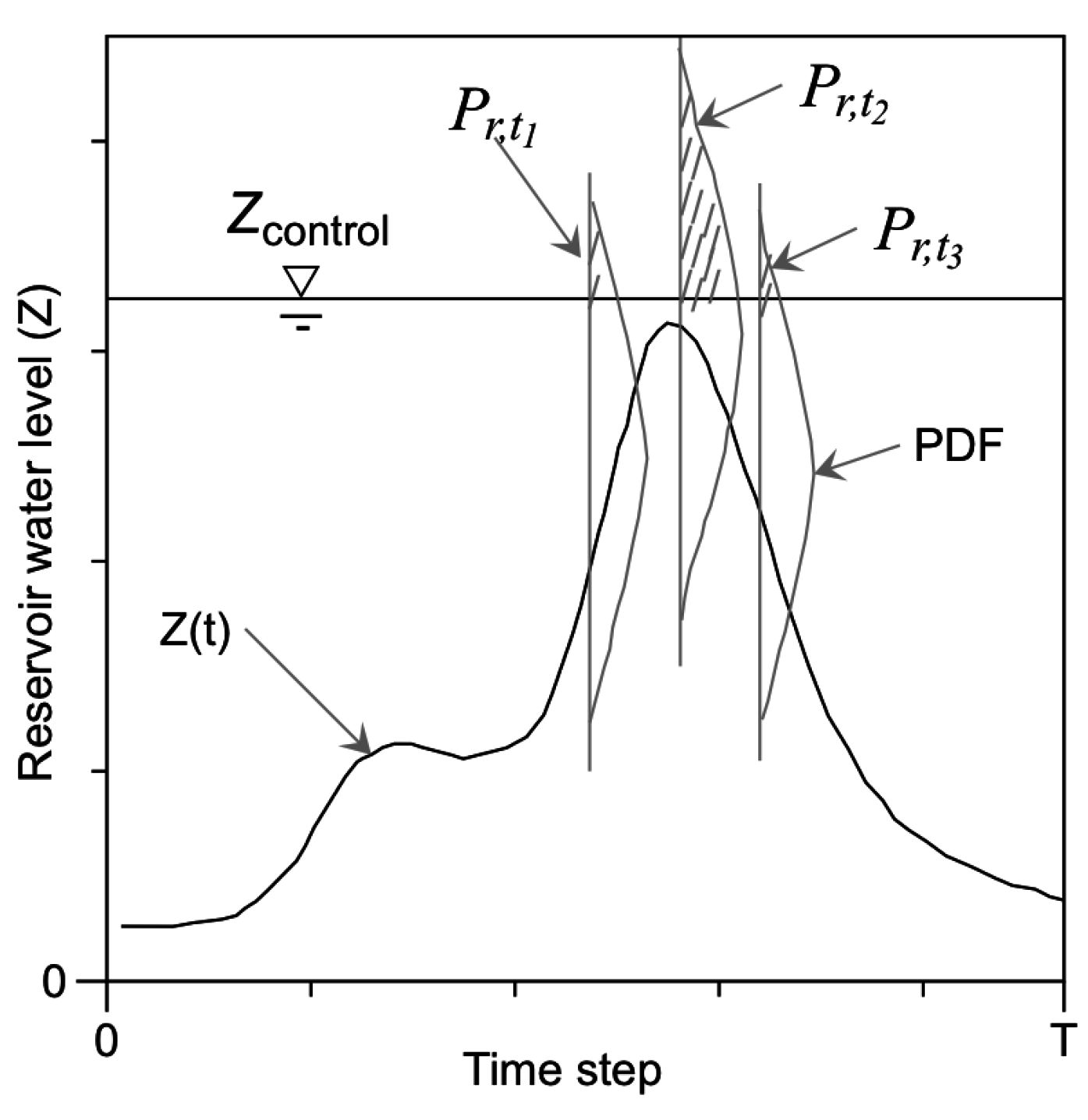
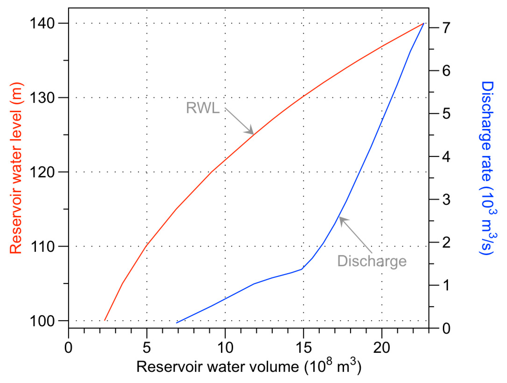
2.4. Risk Rate in Reservoir Flood Routing Calculation

The results of the reservoir flood routing calculation, such as RWL and discharge rate, can be viewed as the random variables when the inflow processes are random. Numerous inflow conditions can be extracted from the probabilistic inflow forecasts for the reservoir flood routing calculation, producing the RWL result that is described with a probability density function (PDF) form. Within one calculating time step ($\Delta t=t_2-t_1$), the water balance of reservoir can be expressed as:

$$\overline{Q}-\overline{q}=\frac{Q_1+Q_2}{2}-\frac{q_1+q_2}{2}=\frac{V_2-V_1}{\Delta t}=\frac{\Delta V}{\Delta t},$$

(9)

where Q₁, q₁, and V₁ are the inflow, discharge rate, and RWV at time t₁, respectively, while Q₂, q₂, and V₂ are the corresponding values at time t₂; $\overline{Q}$ and $\overline{q}$ are the average inflow and outflow of the reservoir in the time step $\Delta t$; and $\Delta V$ is the change of RWV in the time step $\Delta t$. This equation ignores the water traveling time from the points that the basin runoff flows into to the flow-releasing structures. Generally, the relationship between discharge (q) and water level (Z) or water volume (V) can be described with a single function:

q = f(Z) or q = f(V).

(10)

From the start time of reservoir flood routing calculation, Equations (9) and (10) can be solved jointly at each time step, and thus the processes of the RWL and outflow (discharge rate) can be obtained.

Based on the probabilistic inflow forecasts, numerous output conditions (such as RWL) can be calculated and then described in the PDF form at each time step. The risk rate of the reservoir flood routing calculation that describes the probability of RWL greater than a defined safety control water level is described as:

$$P_{r,t}=P\left(Z_t>Z_{control}\right),$$

(11)

where $P_{r,t}$ and Z_t are the risk rate and RWL at time t, respectively; and Z_control is the defined safety control water level that could be set as the characteristic reservoir water level. The generalized concept of “risk” involves not only the flooding probability (i.e., the hazard), but also the exposure loss. The risk rate used here describes the hazard, but no exposure loss was involved. The calculation of risk rates during a reservoir flood routing process is shown in Figure 3. Obviously, when using deterministic inflow process, Z(t), there would not be any risk during the reservoir flood routing calculation. However, there would be the probability of Z_t > Z_control described by PDF of water level at each time step. This probability is different during the reservoir flood routing calculation process, and the maximum value is defined as the risk rate for the entire process:

$$P_r=\max \left(P_{r,1},P_{r,2},\dots ,P_{r,T}\right).$$

(12)

3. Results and Discussion

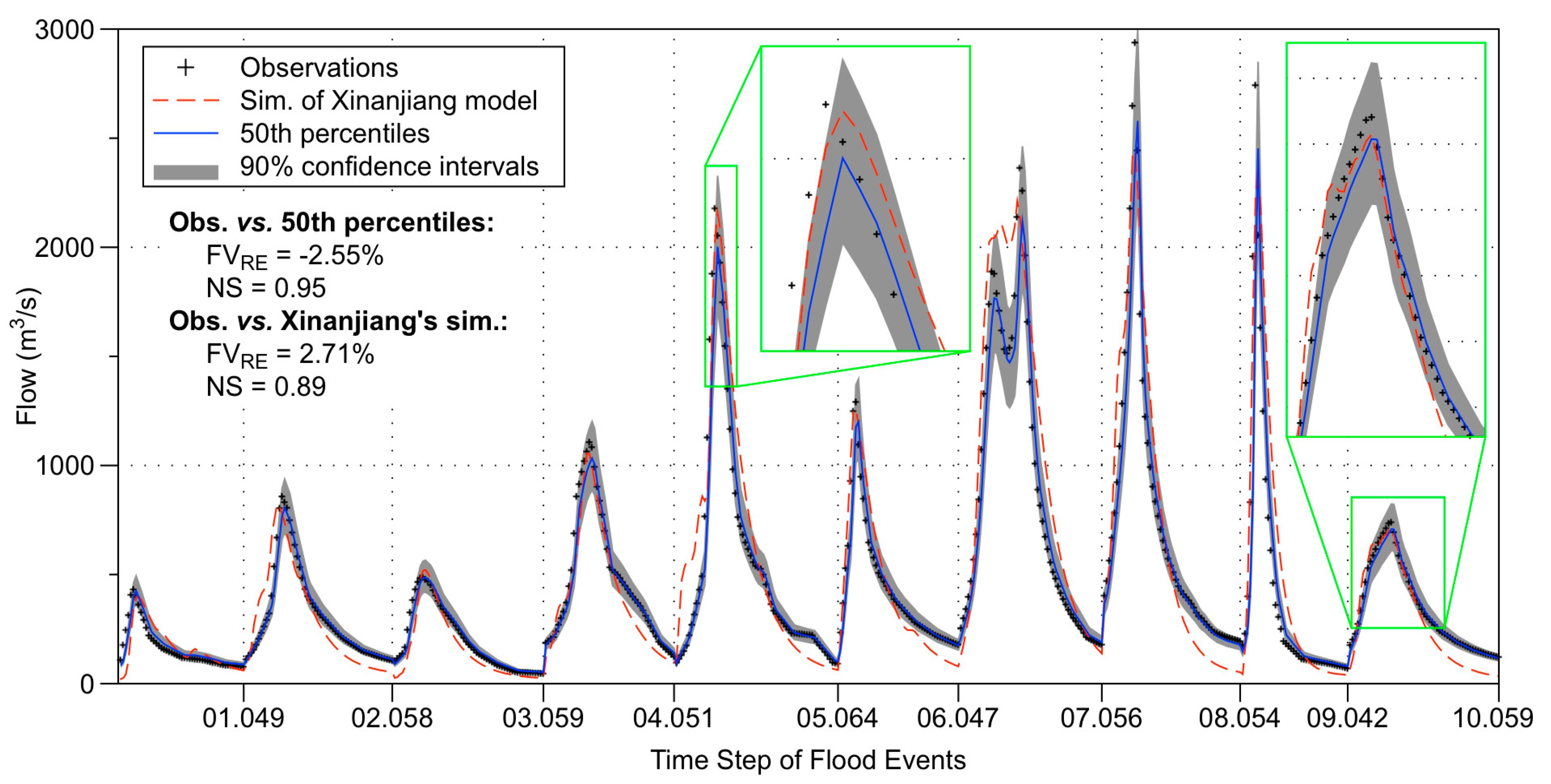
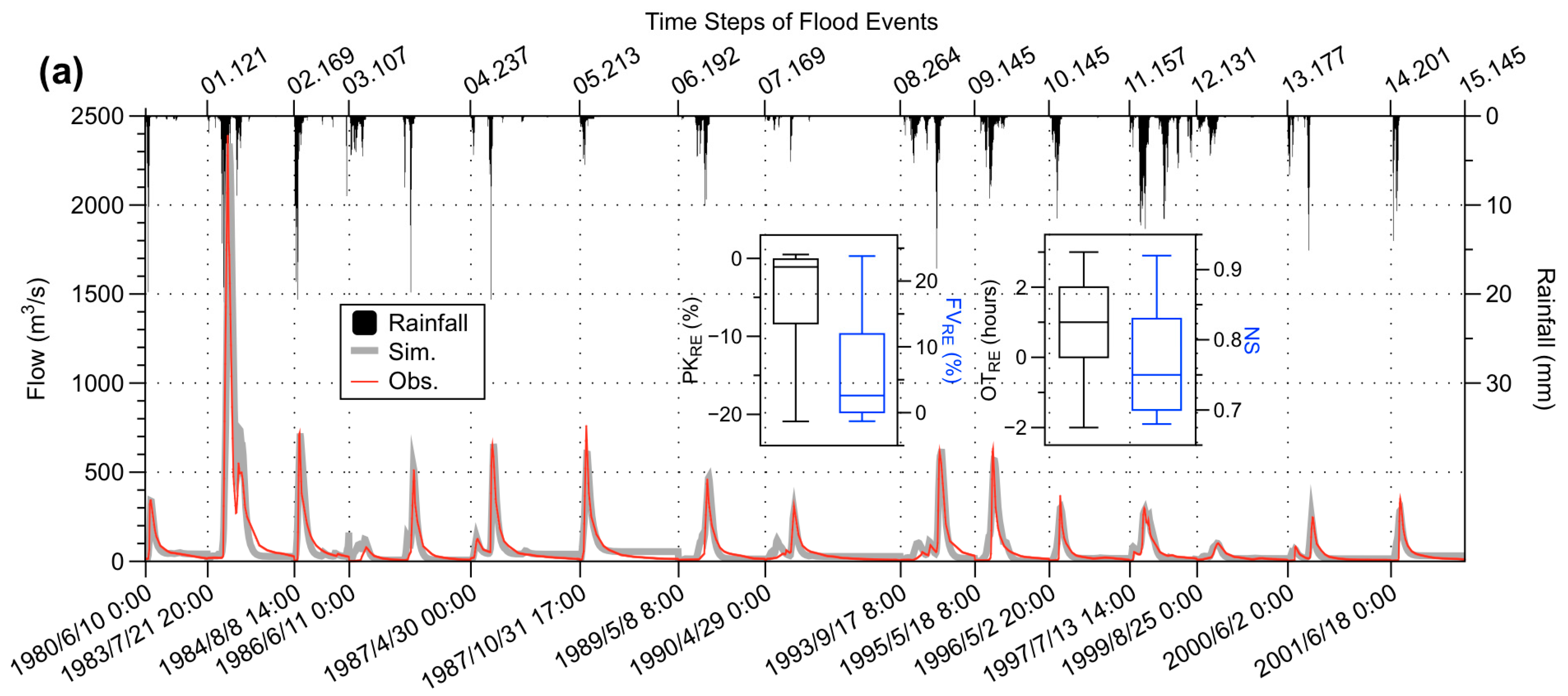
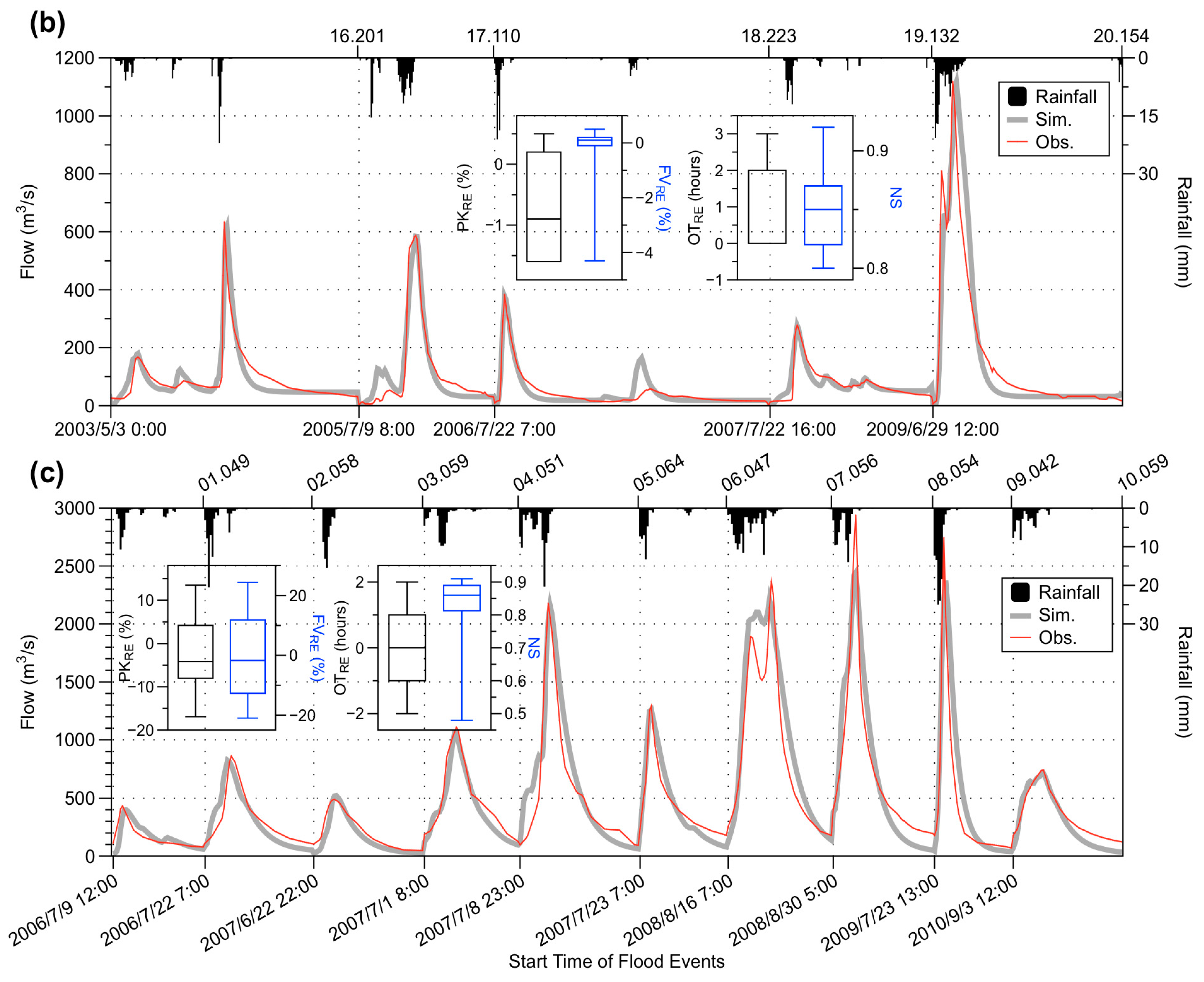
3.1. Calibration and Validation of Xinanjiang Model

Model parameters were calibrated and validated in the drainage area above the Huangnizhuang hydrologic station, and the parameter values are listed in

Table 1. Calibrated parameter values of the Xinanjiang model for flood events shown in Figure 4a.

Evapotranspiration	Runoff Production	Runoff Separation	Runoff Concentration
KC = 0.998	WM = 120 mm	SM = 10 mm	CI = 0.98
WUM = 20 mm	B = 0.4	EX = 1.2	CG = 0.85
WLM = 60 mm	IM = 0.1	KG = 0.45	CS = 0.01
C = 0.2		KI = 0.25	L 1

Notes: ¹ The “lag” parameter, L, is set to 3 h for two upstream sub-basins above the Huangnizhuang station (in the lower left zone of Figure 1), and to one hour for all other sub-basins.

. Figure 4 shows the comparisons between simulated and observed flows at the Huangnizhuang station and the whole Meishan basin. The selected floods for calibration or validation purposes can be identified with starting time and total time steps labeled in the bottom and top abscissae, respectively. The performance was examined with the statistics of peak flow error (relative error, PK_RE, %), flood volume error (FV_RE, %), peak flow occurrence time error (OT_RE, hours) and Nash–Sutcliffe coefficient (NS). In the calibration, the NS varies from 0.68 to 0.92, with an average of 0.78, showing a good agreement with the observed hydrographs (Figure 4a). In the detection of peaks, only one event does not meet the accuracy requirement of |PK_RE| < 20%, and most events have smaller peak errors. Furthermore, the simulated peak occurrence times were also close to the observation, with a maximum bias of 3 h. This proved the applicability of the model in peak detection. In addition, the FV_RE statistic also had acceptable accuracy when only one event moderately exceeded the limit line of |FV_RE| < 20%.

Figure 4b,c show the validation at the Huangnizhuang and Meishan stations, respectively. The validation shows that the average NS statistic of all flood events increased to 0.85 and 0.82 at these two hydrologic stations, respectively. In the validation of the Xinanjiang model at the Huangnizhuang station, the simulated peak flows were very close to the observations in terms of PK_RE and OT_RE measures. It is worth mentioning that PK_RE had a narrower range in validation than in calibration. This may be caused by the relatively smaller number of flood events in the validation than in the calibration period. In addition, the parameter uncertainty in the calibration (and random biases) may provide a better accuracy of a certain index (PK_RE in this case) in the validation. For the Meishan basin, the accuracy of peaks slightly decreased in the measure of PK_RE, but was still within the 20% limit. The difference of model performance between these two hydrologic stations could also be found in the measure of FV_RE. The maximum bias of flood volume at the Huangnizhuang station was FV_RE = −4.3% for the 16th flood event (Figure 4b), while the large biases of the Meishan basin could be found at the 3rd and 9th events (−21.0% and 24.4% for FV_RE, respectively, Figure 4c). As a whole, although there were several large biases in the validations, the calibrated parameters could be assumed reasonable for the Meishan basin with the consideration of all test results.

3.2. Inflow Forecast Uncertainty Analysis

The PFF results of ten flood events at the Meishan station (Figure 4c) can be obtained based on the posterior PDFs of inflow forecast generated by the HUP. Thus, at each time step of flood events, the HUP provides not only the median forecast results (i.e., 50th percentiles) but also the fundamental uncertainty information (e.g., 90% confidence intervals). Figure 5 shows the HUP forecasts and their comparisons with the observations and the simulations of Xinanjiang model in the Meishan basin. Results showed that the 50th percentile forecast strongly agrees with the observations with the performance statistics of FV_RE = −2.55% and NS = 0.95 for all ten flood events. The simulated peaks also showed high accuracies in both the value and corresponding occurrence time, while PK_RE ranged from −12.3% to −0.5% with an absolute value of 6.84%, and the average bias of occurrence time was one hour. Obviously, the mean forecast of HUP showed a better agreement than the Xinanjiang model, whose main biases could be found in low flows and the peak occurrence time.

The uncertainty band of 90% confidence intervals is a good measure for the PFF models. In general, from the whole accuracy of all time steps, we pursue a best uncertainty band that is as narrow as possible but contains as many observations as possible. Thus, two indices can be defined to measure the model forecast uncertainty: the average band width percentage of 90% confidence intervals (BR) and the percentage of the observations bracketed by this band (CR). The measure of BR is defined by averaging the ratios of the difference between 95% and 5% quantiles to observations for all time steps. The measure of CR is also estimated from all time steps. The calculated measures for flood events in Figure 5 were BR = 28.0% and CR = 77.2%. This indicated that most observed flows were contained within the 90% confidence intervals. The exceptions were mainly the high flows caused by the occurrence time biases, but these observations were very close to the uncertainty band. Results proved the applicability of HUP in the Meishan basin.

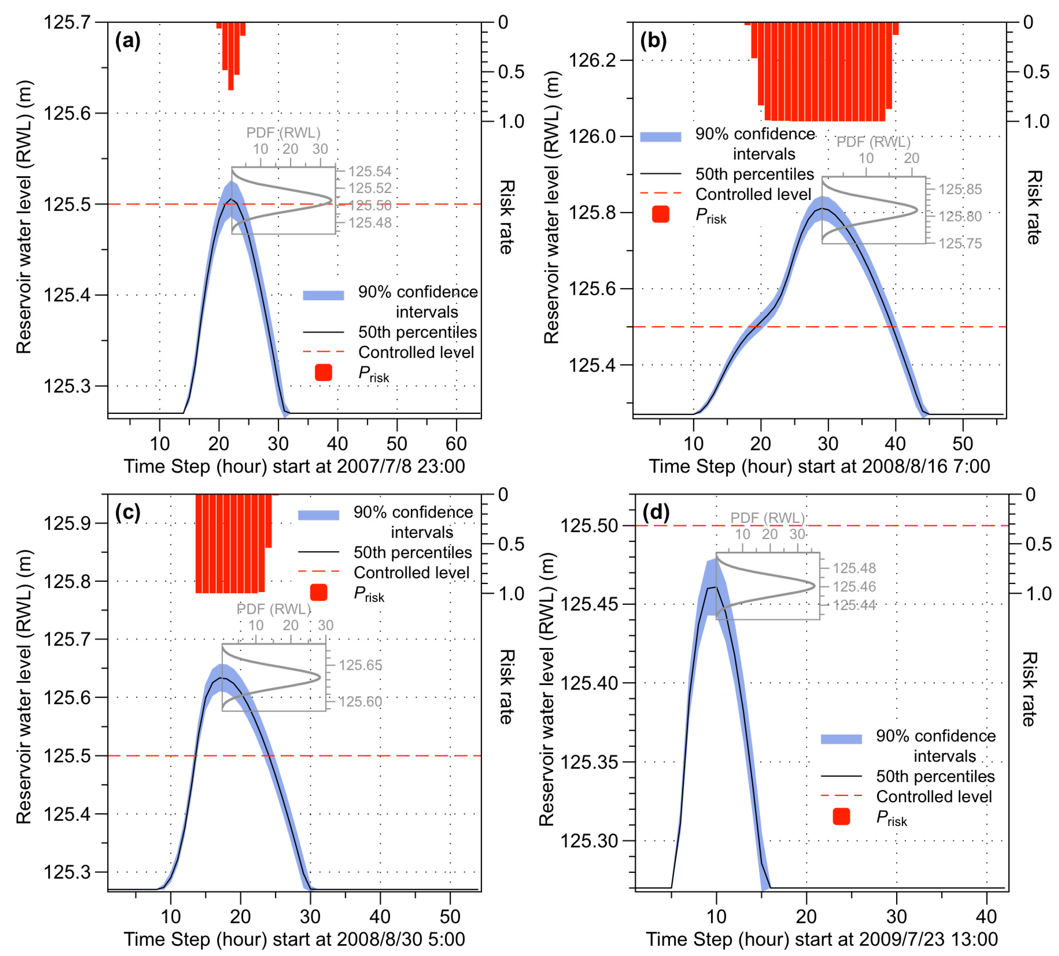
3.3. Risk Rate Calculation

In the operational reservoir scheduling, the flood routing calculation is conducted based on the forecasted inflow data. Thus, the forecasted inflow in the PDF form from the HUP model could be input for the reservoir flood routing calculation. In total, at each time step during a flood event, 1000 flow values were randomly sampled from the posterior PDF of forecasted inflow, and thus 1000 sets of inflow hydrographs were obtained for reservoir flood routing calculation. Furthermore, the corresponding 1000 sets of RWL could be simulated at each time step according to the regulation rules of the main flood season, and an initial RWL value that equals the FLWL (125.27 m) in most situations during flood seasons. Thus, the PDFs of RWL could be derived from the samples and be further used for risk rate calculation. Results showed that floods with low magnitude of flow cannot always cause the changes of RWL, because all inflow volume were released from the reservoir when inflow <1200 m³/s for all time steps. Thus, only four events with relatively large flows (i.e., the 5th, 7th, 8th, and 9th floods) are shown in Figure 6. At each time step, both deterministic and probabilistic forecasts (such as the 50th percentiles and 90% confidence intervals, respectively) could be obtained based on the PDFs of RWL. Results suggested that the forecast uncertainty increased from low to high RWL values, indicating by the width of uncertainty band.

Combined with the safety control water level (Z_control), the risk rates can be calculated. In general, the Z_control value is defined as a characteristic reservoir water level; e.g., top level of flood control, design flood level, or check flood level. For the cases in this study, however, the possible RWL values of all selected flood events (derived from its PDF) were far less than these characteristic levels; i.e., P_r = 0 (no risk). In order to demonstrate the risk rate calculation procedure, we defined the Z_control value as a relatively low water level (Z_control = 125.5 m) and calculated the risk rate at each time step (Figure 6). Results suggested that the risk rate largely depends on the forecast uncertainty of RWL. High flows and wide uncertainty bands were more likely to produce high risk rates, such as the 7th flood shown in Figure 6b. As a negative example, in the 9th flood, the PDF of RWL at peak time indicated that RWL had no possibility of reaching the safety control water level, and thus the risk rate for this flood was zero. The risk rates of the reservoir flood routing calculation could provide reliable references for flood control and reservoir regulation decision-making.

4. Conclusions

The complexity of hydrologic processes determines the objective existence and inevitability of hydrologic forecast uncertainties. Deterministic flood forecasts cannot lead to an objective evaluation of the possible risks in reservoir flood routing calculation. On the contrary, PFF could provide not only the median forecast results, but also the fundamental uncertainty information (such as the PDF of flow at each time), and further serves as the input of the calculations of reservoir flood routing and risk rate. In this paper, we presented a risk analysis of reservoir flood routing calculation based on inflow forecast uncertainty in the Meishan Reservoir of Huaihe River, China. The main conclusions can be drawn as follows. (1) The Xinanjiang model was used as a deterministic hydrologic model to simulate the flood inflows to the Meishan Reservoir. According to the data condition and hydrologic similarity, the Xinanjiang model was calibrated and validated at the Huangnizhuang station, and results showed that the performance measures of peak, volume, and process (PK_RE, OT_RE, FV_RE, and NS) meet the accuracy requirements. In addition, the validation in the entire Meishan basin also proved the model applicability in the reservoir inflow forecasts; (2) The total uncertainty (except for the input uncertainty) in the inflow forecasts was quantified by the HUP model, providing the PDF of inflow and corresponding PFF results (e.g., 90% confidence intervals) at each time step; (3) Based on the posterior PDFs of inflow forecasts derived by the HUP model, a large number of inflow samples that were randomly extracted from inflow’s PDF could generate the RWL (and its PDF) during flood events through the reservoir scheduling simulation. Thus, the risk rate of RWL exceeding the safety control level (Z_control) could be calculated for the references in the reservoir flood control and regulation decision-making.

References

1. Mendoza, P.A.; McPhee, J.; Vargas, X. Uncertainty in flood forecasting: A distributed modeling approach in a sparse data catchment. Water Resour. Res. 2012, 48, W09532. [Google Scholar] [CrossRef]
2. Beven, K.; Jim, H. Applied Uncertainty Analysis for Flood Risk Management; World Scientific: London, UK, 2014. [Google Scholar]
3. Ajami, N.K.; Duan, Q.; Sorooshian, S. An integrated hydrologic Bayesian multimodel combination framework: Confronting input, parameter, and model structural uncertainty in hydrologic prediction. Water Resour. Res. 2007, 43, W01403. [Google Scholar] [CrossRef]
4. Li, B.; Yu, Z.; Liang, Z.; Song, K.; Li, H.; Wang, Y.; Zhang, W.; Acharya, K. Effects of climate variations and human activities on runoff in the Zoige alpine wetland in the eastern edge of the Tibetan Plateau. J. Hydrol. Eng. 2014, 19, 1026–1035. [Google Scholar] [CrossRef]
5. Liu, Z.; Guo, S.; Zhang, H.; Liu, D.; Yang, G. Comparative study of three updating procedures for real-time flood forecasting. Water Resour. Manag. 2016, 30, 2111–2126. [Google Scholar] [CrossRef]
6. Li, B.; Liang, Z.; He, Y.; Hu, L.; Zhao, W.; Acharya, K. Comparison of parameter uncertainty analysis techniques for a TOPMODEL application. Stoch. Environ. Res. Risk Assess. 2016. [Google Scholar] [CrossRef]
7. Beven, K.; Binley, A. The future of distributed models: Model calibration and uncertainty prediction. Hydrol. Process. 1992, 6, 279–298. [Google Scholar] [CrossRef]
8. Krzysztofowicz, R. Bayesian theory of probabilistic forecasting via deterministic hydrologic model. Water Resour. Res. 1999, 35, 2739–2750. [Google Scholar] [CrossRef]
9. Bates, B.C.; Campbell, E.P. A Markov Chain Monte Carlo Scheme for parameter estimation and inference in conceptual rainfall-runoff modeling. Water Resour. Res. 2001, 37, 937–947. [Google Scholar] [CrossRef]
10. Kuczera, G.; Kavetski, D.; Franks, S.; Thyer, M. Towards a Bayesian total error analysis of conceptual rainfall-runoff models: Characterising model error using storm-dependent parameters. J. Hydrol. 2006, 331, 161–177. [Google Scholar] [CrossRef]
11. Xiong, L.; Wan, M.; Wei, X.; O’connor, K.M. Indices for assessing the prediction bounds of hydrological models and application by generalised likelihood uncertainty estimation. Hydrol. Sci. J. 2009, 54, 852–871. [Google Scholar] [CrossRef]
12. DeChant, C.M.; Moradkhani, H. On the assessment of reliability in probabilistic hydrometeorological event forecasting. Water Resour. Res. 2015, 51, 3867–3883. [Google Scholar] [CrossRef]
13. Todini, E. History and perspectives of hydrological catchment modelling. Hydrol. Res. 2011, 42, 73–85. [Google Scholar] [CrossRef]
14. Ouarda, T.B.M.J.; Labadie, J.W. Chance-constrained optimal control for multireservoir system optimization and risk analysis. Stoch. Environ. Res. Risk Assess. 2001, 15, 185–204. [Google Scholar] [CrossRef]
15. Ding, W.; Zhang, C.; Peng, Y.; Zeng, R.; Zhou, H.; Cai, X. An analytical framework for flood water conservation considering forecast uncertainty and acceptable risk. Water Resour. Res. 2015, 51, 4702–4726. [Google Scholar] [CrossRef]
16. Zhang, M.; Yang, F.; Wu, J.X.; Fan, Z.W.; Wang, Y.Y. Application of minimum reward risk model in reservoir generation scheduling. Water Resour. Manag. 2016, 30, 1345–1355. [Google Scholar] [CrossRef]
17. Jonkman, S.N.; van Gelder, P.H.A.J.M.; Vrijling, J.K. An overview of quantitative risk measures for loss of life and economic damage. J. Hazard. Mater. 2003, 99, 1–30. [Google Scholar] [CrossRef]
18. Zhao, R.J. Flood Forecasting Method for Humid Regions of China; East China College of Hydraulic Engineering: Nanjing, China, 1977. [Google Scholar]
19. Zhao, R.J. The Xinanjiang model applied in China. J. Hydrol. 1992, 135, 371–381. [Google Scholar]
20. Wang, J.; Liang, Z.; Jiang, X.; Li, B.; Chen, L. Bayesian theory based self-adapting real-time correction model for flood forecasting. Water 2016, 8, 75. [Google Scholar] [CrossRef]
21. Huaihe River Water Resources Commission. Handbook for Flood Control and Drought Relief of the Huaihe River Basin; Huaihe River Water Resources Commission: Bengbu, China, 2014. [Google Scholar]
22. Liang, X.; Lettenmaier, D.P.; Wood, E.F. One-dimensional statistical dynamic representation of subgrid spatial variability of precipitation in the two-layer variable infiltration capacity model. J. Geophys. Res. 1996, 101, 21403–21422. [Google Scholar] [CrossRef]
23. Todini, E. The ARNO rainfall-runoff model. J. Hydrol. 1996, 175, 339–382. [Google Scholar] [CrossRef]
24. Liang, Z.; Wang, J.; Li, B.; Yu, Z. A statistically based runoff-yield model coupling infiltration excess and saturation excess mechanisms. Hydrol. Process. 2012, 26, 2856–2865. [Google Scholar] [CrossRef]
25. Krzysztofowicz, R.; Herr, H.D. Hydrologic uncertainty processor for probabilistic river stage forecasting: Precipitation-dependent model. J. Hydrol. 2001, 249, 46–68. [Google Scholar] [CrossRef]
26. Krzysztofowicz, R.; Kelly, K.S. Hydrologic uncertainty processor for probabilistic river stage forecasting. Water Resour. Res. 2000, 36, 3265–3277. [Google Scholar] [CrossRef]
Figure 1. Location of the Meishan Reservoir and its drainage basin.
Water 08 00486 g001
Figure 2. Relationship between water level, water volume and discharge rate of the Meishan Reservoir. RWL: reservoir water level.
Water 08 00486 g002
Figure 3. Sketch of the calculation of risk rates during a reservoir flood routing process. PDF: probability density function.
Water 08 00486 g003
Figure 4. Comparisons between simulated and observed flows of flood events: (a) calibration at the Huangnizhuang station; (b) validation at the Huangnizhuang station; and (c) validation in the entire Meishan basin. The box-plots present the distributions of four statistics (peak flow error, PKRE; flood volume error, FVRE; peak flow occurrence time error, OTRE; and Nash–Sutcliffe coefficient, NS) for all considered flood events. The numbers on the top axes—with the two-digit format for flood ID and three-digit for ending time step—separate the artificially attached series of flood events.
Water 08 00486 g004aWater 08 00486 g004b
Figure 5. Hydrologic Uncertainty Processor (HUP) forecasts compared to the observations and the simulations of Xinanjiang model. Green boxes magnify the zone of peak time steps. The same flood events are used as shown in Figure 4c. The numbers on the bottom axes—with the two-digit format of for flood ID and three-digit for ending time step—separate the artificially attached series of flood events.
Water 08 00486 g005
Figure 6. Risk rate calculation of selected flood events for the Meishan Reservoir. The grey small graph is the probability density function (PDF) of reservoir water level (RWL) at the peak occurrence time step.
Water 08 00486 g006