Article

Nonlinear Changes in Land Cover and Sediment Runoff in a New Zealand Catchment Dominated by Plantation Forestry and Livestock Grazing

1
Department of Geography, Texas State University, San Marcos, TX 78666, USA
2
Landscape & Land Use Change Institute (LLUCI), Norman, OK 73069, USA
3
National Institute of Water and Atmospheric Research (NIWA), Hamilton, 3216, New Zealand
4
Department of Geography and Environmental Sustainability, University of Oklahoma, Norman, OK 73019, USA
*
Author to whom correspondence should be addressed.
Water 2016, 8(10), 436; https://doi.org/10.3390/w8100436
Submission received: 30 July 2016 / Accepted: 23 September 2016 / Published: 4 October 2016
(This article belongs to the Special Issue Land Use, Climate, and Water Resources)

Abstract

:
Land cover can change frequently on intensively managed landscapes, affecting water quality across different spatiotemporal scales. Multi-resolution datasets are necessary in order to assess the extent and trends of these changes, as well as potential cross-scale interactions. In this study, both spatial and temporal analyses of land disturbance (i.e., soil exposure from vegetation removal) and water quality were performed on datasets ranging from daily to yearly time scales. Time-series analyses of land disturbance were compared against the water quality variables of total suspended solids (TSS), turbidity, and visual clarity for the Hoteo River catchment on the North Island of New Zealand for the 2000–2013 period. During forest harvest and recovery phases, exotic forests were the dominant disturbance, up to five times the area of grassland disturbance; while after recovery, grasslands assumed the dominant role, for up to 16 times the area of forest disturbance. Time-series of TSS from field sampling (2000–2013) and TSS-event analyses (2012–2014) displayed distinct nonlinear patterns, suggesting that after major events, sediment that is stored in the landscape is exhausted and a period of sediment build-up follows until the next major event. Time-series analyses also showed a connection between trends in connected land disturbance and visual water clarity, with connected disturbance having the potential to be a water quality indicator. Future research should be conducted at even finer spatiotemporal scales over longer periods in order to identify effects of localized land disturbances on downstream water quality.

1. Introduction

Of all the landscape components, land use has had the greatest impact on water quality over the past couple of centuries [1,2]. Accordingly, a principal point of focus in water resources and fluvial geomorphic investigations is how land cover/land use change (LCLUC) affects water quality of freshwater ecosystems, particularly suspended sediment dynamics. Understanding how LCLUC affects sediment runoff requires three pieces of information: (1) how the land use affects available sediment for runoff; (2) how the land use interacts with other landscape components to mitigate or enhance sediment runoff; and (3) connectivity between available sediment from land use and the drainage network. When all three of these processes are considered together, the relationships between LCLUC and fluvial sediment regimes are likely to be nonlinear over both space and time [3,4].
While these nonlinearities have been theorized for geomorphic systems [5], rarely (if ever) have nonlinearities in suspended sediment (other than event-scale hysteresis effects) been empirically connected to LCLUC. The reasons are twofold. First, most studies only consider one—or at most two—of the “three pieces of information” mentioned above [6,7]. Second, the required data to capture these phenomena are usually not available at the appropriate spatio-temporal resolution. For example, temporal resolution of readily-available land cover datasets usually limits researchers to assessing land cover/use on decadal or semi-decadal time-scales [8,9], when in reality, it can change on a weekly to monthly scale [10,11]. Spatially, suspended sediment or the related optical water quality variables of turbidity and visual water clarity are usually measured only at the catchment outlet, which can hide the effects of specific land–water relationships [12], although there are exceptions where sub-catchment analyses were conducted [13,14]. Further, only a few monitoring programs worldwide have consistently measured fluvial sediment in short intervals over long periods.
Sediment production from the drainage basin occurs when the force of water (via precipitation or flow) encounters available sediment. If vegetation is removed from the soil surface, it is more likely to be eroded [15,16]. Two common land uses that remove vegetation are plantation forestry harvesting and livestock grazing. After harvesting in plantation forestry, the soil (which typically lacks understory vegetation in forests with dense canopy) is left exposed. It is then readily available to be washed off during the next high precipitation event, resulting in considerable amounts of sediment and other materials entering the stream [17,18,19]. Other major sources of erosion/runoff in plantation forests include roads (and their sidecast), landing sites, shallow landslides, and channel scouring/gullying [20,21,22]. Similar processes, but at a finer spatial scale, can take place with intensive grazing [23,24,25], particularly where rotational paddocks are cyclically grazed to bare ground and left to recover. The recovery time depends on weather conditions and soil moisture/fertility [26]. The likelihood of exposure to precipitation increases with recovery time; thus, the chances of transporting sediment to riverine systems increases as management-intensive grazing expands and intensifies.
The relationship between LCLUC and sediment production depends on additional landscape characteristics such as slope, aspect, drought, soil properties, and vegetation. The relationship between hillslope erosion potential and vegetation, in particular, is complex and likely involves cross-scale interactions (i.e., when processes at one spatial or temporal scale interact with processes at finer or broader scales [27]) because of their inherent interdependency [28]. However, in general, when vegetation cover increases, hillslope erosion potential decreases, and vice versa [15,28]. Aspect affects vegetation vigor and recovery time, as south-facing slopes receive less sunshine than north-facing slopes in the southern hemisphere (opposite for the northern hemisphere). Prolonged periods of drought may also increase hillslope erosion potential by causing vegetation die-off or slowing recovery times. Soil properties such as texture dictate fertility and moisture, with loamy soils usually being the most beneficial. However, loamy soils can be more erodible compared to sandy and clayey soils [29].
In order to understand the interaction between LCLUC and sediment production, river–landscape connectivity must be established, which requires an accurate stream channel network that includes even intermittent and ephemeral channels [30]. Once the stream channel network is properly characterized, critical source areas of sediment (CSAS) can be derived. The most common stream delineation methodology employed by watershed/catchment models is the minimum area threshold method; however, different landscape characteristics produce different channel initiation thresholds [31,32]. Uniformly applying the same area threshold across physiographically diverse landscapes can result in considerable under- or over-estimation of stream density [30,33]. After mapping an accurate channel network, landscape connectivity (via CSAS) is then determined by adjacent surface runoff from hillslopes and floodplains [31,32,34]. Previous attempts to assess landscape connectivity included computer- and field-based numerical assessments [35] and elaborate conceptual frameworks of hydrological and sediment connectivity [36,37]. However, there are simpler procedures to determine connectivity, such as the one from Palmer et al. [38] that is based on slope thresholds, flow direction, and proximity to the drainage network. When a connected area is disturbed, it is considered to be a CSAS. These catchment-scale hydrographic methods allow us to assess the impact of landscape disturbances on long-term trends in river water quality; specifically, total suspended solids (TSS), turbidity, and visual water clarity.
Our understanding of water cycles and sediment erosion/transportation has demonstrated that there is not always a linear relationship between water quality and land management practices [3,34]. For example, in order for elevated turbidity values to be recorded at a monitoring site, “adequate” amounts of precipitation must mobilize readily available sediment throughout the landscape. Not only is there variation in precipitation across the catchment, but also in antecedent soil moisture conditions, in water abstraction for irrigation, and in the spatiotemporal scale of the data analyzed [39]. Even after all the aforementioned are taken into consideration, not all available sediment is delivered to the channel immediately (i.e., it can be stored and released at a later time) [40,41]. These lag and legacy effects can further enhance nonlinear LCLUC–sediment runoff relationships. In order to capture these potentially nonlinear changes, high-resolution spatiotemporal data is needed.
In this study, we take advantage of a high temporal-resolution (8-day) land cover dataset over 14 years (2000–2014) and multiple water quality datasets with multiple sampling intervals (5-minute to monthly) over the same period, distributed throughout the catchment in order to examine connections among LCLUC, connectivity, and sediment runoff. The aim of this paper is fourfold: (1) understand how different land uses—specifically livestock grazing and forest harvesting—affect sediment runoff at the sub-catchment scale; (2) assess how land cover interactions with other landscape components influence sediment runoff regimes; (3) determine landscape connectivity between available sediment and the drainage network; and (4) characterize long-term trends in suspended sediment at the catchment scale. Suspended sediment data (interpolated from continuous turbidity records) was used to create time-series, derive suspended sediment budgets, and locate the sources and land uses responsible for increased sediment yields to the river system. Statistical analysis (i.e., piecewise regression) of water quality and land disturbance time-series at a monthly scale was then performed to assess the nonlinear trends and connections between landscape changes and river sediment regimes.

2. Materials and Methods
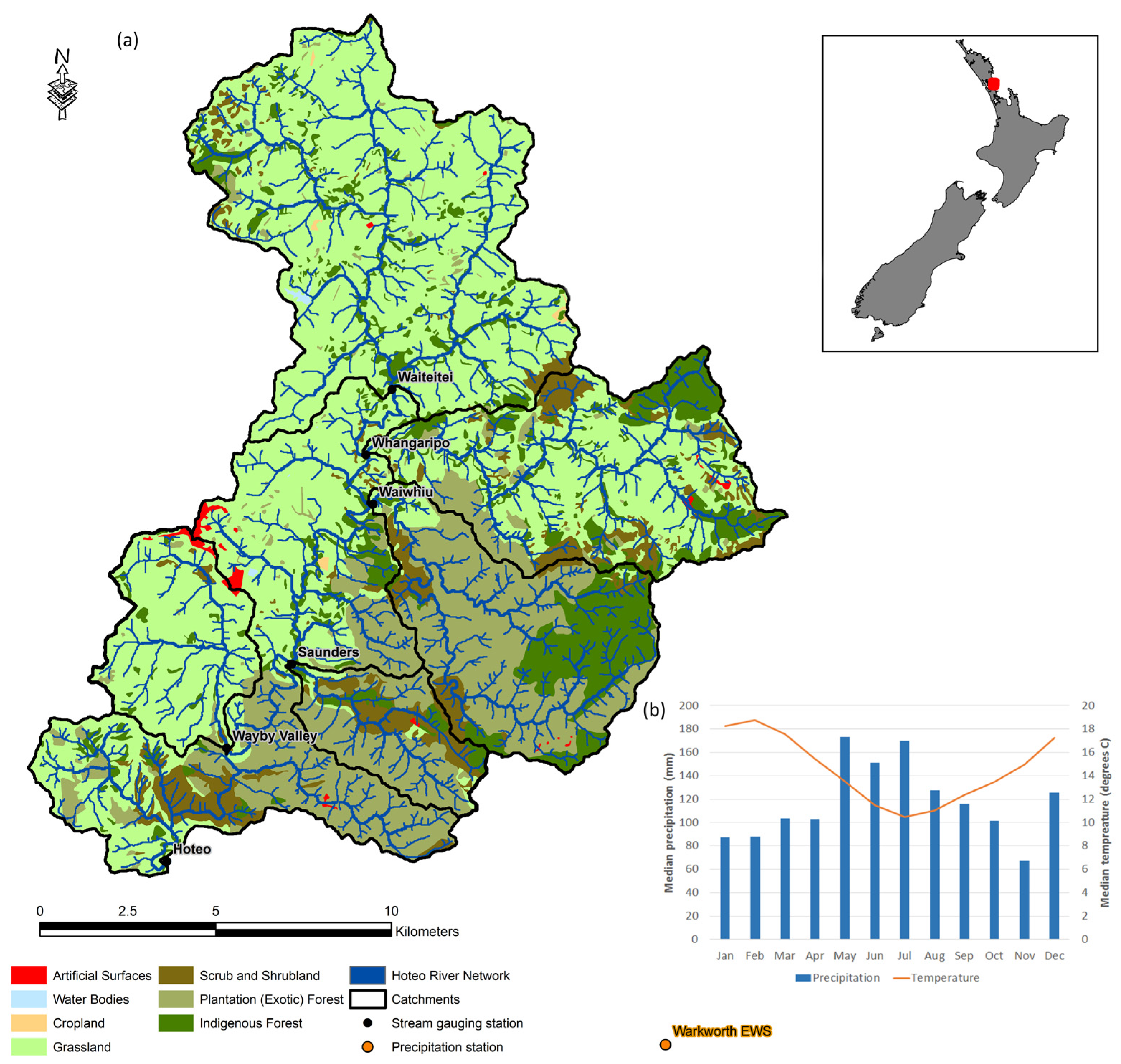
2.1. Study Area

For this study we selected a catchment with all of the previously described data requirements, in addition to having large areas of both plantation forestry and livestock grazing. The Hoteo River catchment is located in the northern part of New Zealand’s North Island, approximately 60 km north of Auckland (Figure 1), and drains to the Kaipara Harbor, which is a valuable and sensitive estuarine ecosystem that is experiencing considerable sediment infilling and associated environmental degradation. The climate of the region is “sub-tropical”, characterized by warm, humid summers and mild winters. Maximum and minimum daily air temperature averages 18.5 °C and 10.1 °C, respectively, with an average of 2129 sunshine hours/year. Most rainfall occurs in sustained events during the winter months of June (155 mm), July (180 mm), and August (152 mm), with an annual total rainfall of 1454 mm (1981–2010, The National Climate Database). Significant differences in precipitation patterns may occur within the catchment due to topography. Buikema (2012) [42] reported variations (±100 mm) in recorded precipitation between the Dome Ranges in the southeastern part of the catchment to the rolling hills in the northwest.
The study area has three distinct landscape units as defined by Buikema (2012): the uplands (with steep slopes, >26°), foothills/rolling foothills, and alluvial floodplains. The dominant soil type is silt- or clay-loams, with the rest silt/sands and silt/clay loams in the river valleys. The original land cover of the catchment has been highly modified since broad-scale European settlement/agriculture in the mid-1800s, with clearings of native forests and draining of wetlands. These clearings have resulted in an increase in gully/channel formation and thus greater landscape connectivity [42].
Present-day land use is characterized by three distinctive classes: (1) grasslands for livestock grazing (dairy/beef cattle, sheep); (2) plantation (exotic) forests; and (3) native forests. Plantation forests are exclusively Monterey pine (Pinus radiata), which are mechanically clear-cut every 28 years, on average. There are a variety of grasses, such as perennial ryegrass, cocksfoot, tall fescue, and kikuyu. Native forests are predominantly podocarp/broad leaf forest [42]. Wildfires in the Hoteo catchment are rare. Land use and other physiographic data for Hoteo and its sub-catchments examined here are summarized in Table 1, and described in detail below.
We divided Hoteo into five sub-catchments based on the locations of monitoring sites within the catchment, resulting in different elevation, slope, and land cover characteristics: Waiteitei, Whangaripo, Waiwhiu, Wayby Valley, and Saunders (Table 2). Waiteitei and Wayby Valley have flat-to-gentle slopes with grasslands being the dominant land cover (>90%). Whangaripo and Waiwhiu have steeper mean slopes (23.2° and 30.3°, respectively), but with different dominant land cover (grassland vs. exotic/native forest). Last, Saunders is also very steep, with an average slope of 28.1° and exotic forestry dominating the land cover.

2.2. Land Cover/Use and Disturbance Index

Land cover and use was characterized with the New Zealand Land Cover Database (LCDB) [8], which we also used to mask out areas other than forests and grasslands. In order to assess land disturbance (times and areas of bare ground), we used an 8 day, 450 meter land cover dataset developed by de Beurs et al. (2016) [10]. Details of the methodology can be found in their paper, but briefly, for each Moderate Resolution Imaging Spectroradiometer (MODIS) image, the Tasseled Cap transformation was calculated; by using the brightness, greenness, and wetness components based on the coefficients from Lobser and Cohen (2007) [43], a disturbance index (DI) (Table 1) was calculated for every pixel. Each component is associated with a landscape property: brightness is linked to albedo, greenness is linked to vegetation vigor, and wetness to the amount of water retained by vegetation. Next, the mean and standard deviation of each landcover and climatic region was calculated to standardize the DI values. The forest DI was calculated as the brightness minus the greenness and wetness; disturbed forests appear more bright but less green and wet compared to undisturbed forests. The grassland index was calculated by taking the negative sum of brightness, greenness, and wetness; disturbed grasslands appear less dark, green, and wet compared to healthy grasslands. The higher the DI, the more sparsely vegetated the pixel was, with a threshold value of three or higher indicating bare ground. We aggregated this dataset by sub-catchment so that our final product was an 8 day time-series (2000–2013) with the percentage of each sub-catchment disturbed (DI > 3).
The 8 day temporal and 450 m spatial resolution over 14 years resulted in a highly detailed land use/cover dataset adequate for the detection of weekly to monthly changes, particularly useful for assessing landscape changes associated with an intensively managed landscape. The index was calculated only on areas that were designated as high-producing grasslands or exotic forestry. Native forests were not assessed, because they were mixed in type and density, and thus displayed false disturbances. The rest of the classes—wetland/open water (0.30%), urban (0.25%), cropland (0.12%), and other (0.07%)—were masked out and not taken into account in DI calculations. For each exotic forest pixel, the time of harvest was identified based on an iterative script that recorded the first date that DI > 3, the sum of dates while DI > 3, and the first date after harvest that DI < 3. This process resulted in a dataset that showed the year of first harvest, duration of recovery, and year of recovery.

2.3. Physiographic Data

A 15 m DEM was acquired from Landcare Research from which slope, direction of flow, and flow accumulation were derived to model catchment connectivity. The DEM was resampled at 450 m to match the DI data. Soils data was obtained from the 1:63,360 Fundamental Soils Layers (FSL), which is maintained by Landcare Research [44]. Soil variables that we included in our analysis were texture and soil moisture.

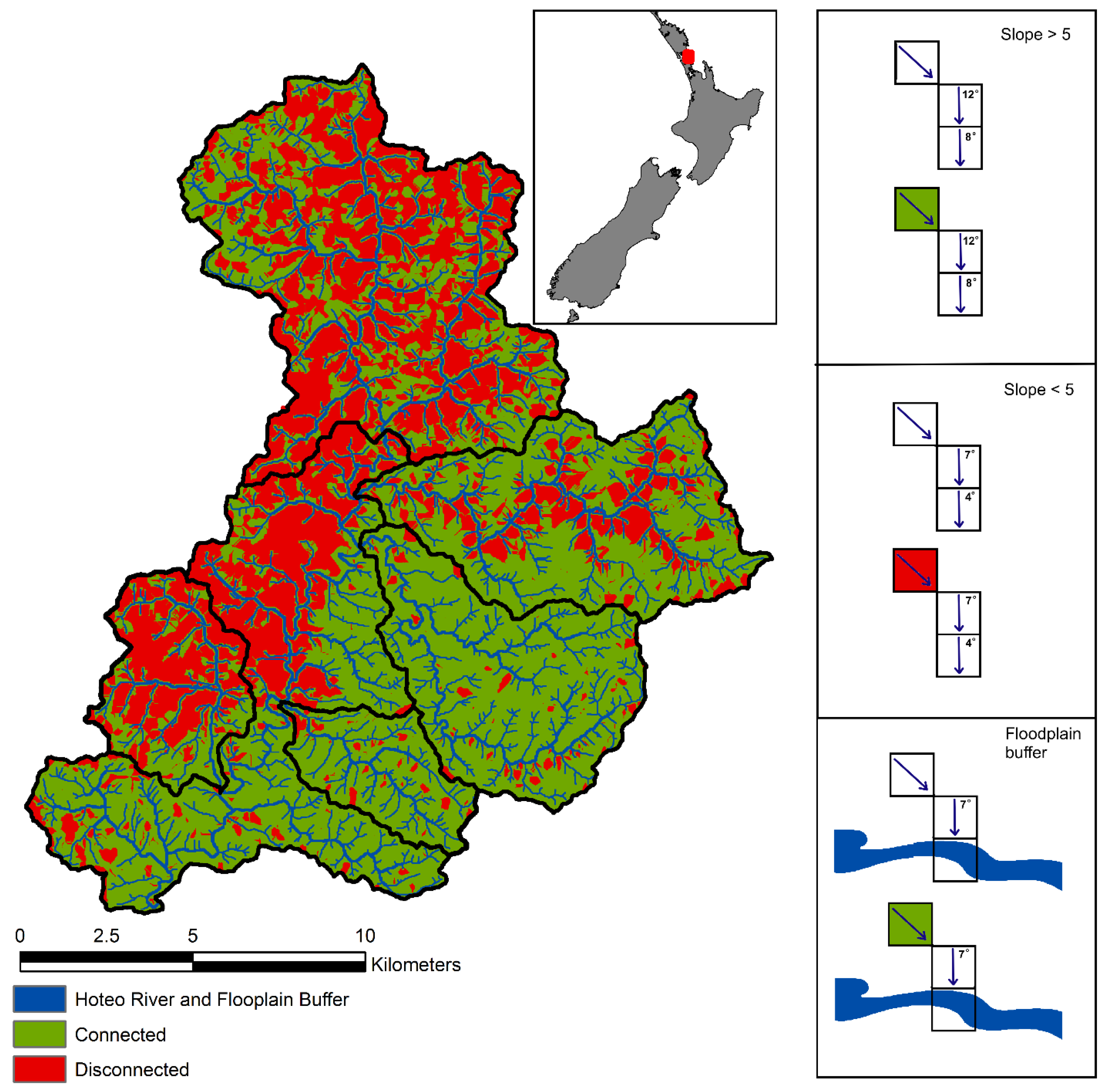
2.4. River Network and Connectivity

The River Environment Classification (REC) is a national-scale (for New Zealand) synthetic stream network derived from a hydrologically corrected DEM [45]. Utilizing “fixed” thresholds on flow accumulation layers to identify the location of channel heads (like REC) is computationally efficient over large areas, but with limitations on the accuracy of the headwater locations [30]. For that reason, we identified all channel heads of the Hoteo catchment using 0.5 m rural aerial photos from 2010–2012 (Land Information New Zealand; LINZ) as reference. Then, using a modified stream delineation algorithm (based on flow direction), we were able to delineate streams from their mapped headwaters to the watershed outlet. The newly-created stream network was used as input to inform the variables of our landscape connectivity model, described below.
We developed a landscape connectivity model in an effort to identify critical source areas of sediment (CSAS). The distinction between CSAS (connected) and areas not contributing to sediment runoff (disconnected) was made based on a sediment runoff model that utilized slope thresholds to allow for sediment movement [38]. Below, we provide a description of the rules applied to each 15 m pixel in order to derive the landscape connectivity mask:
  • Pixels with slope >5° along the flow direction were assigned a “connected” value.
  • If slope <5° for at least two 15 m pixels along the flow direction, then a “non-connected” value was assigned.
  • Pixels immediately adjacent to the river (within the floodplain buffer) were assigned a “connected” value, regardless of slope.
The floodplain buffer was simulated based on the Strahler stream order, and was defined as 30 m for 1st and 2nd stream orders, 60 m for 3rd and 4th stream orders, and 90 m for 5th and 6th stream order, on each side. These buffers were estimated based on the geomorphic mapping of rivers in the catchment by Buikema [42].

2.5. Hydrologic and Water Quality Data

Multiple water quality variables were assessed to estimate total suspended solids (TSS) loads. Monthly visual water clarity at the catchment outlet (Hoteo station) from the National River Water Quality Network (NRWQN) [46] was used because of its consistency and long record (1989–2014), and because it has been proven to be the best estimator of TSS in the absence of TSS samples [47]. Turbidity was used because it is conveniently monitored with in situ sensors that can estimate TSS with high temporal resolution. Although less correlated to TSS than visual water clarity, it is still strongly correlated [47]. Turbidity (in NTU) was monitored at three sites within the catchment (Waiteitei, Waiwhiu, Hoteo) with 5 min resolution for the period 2012–2014. Time-stamped turbidity values were averaged to daily values and converted to TSS based on turbidity–TSS relationships (Gubbs: n = 33, R2 = 0.96, SE = 29.7; Waiteitei: n = 142, R2 = 0.95, SE = 31.0; Waiwhiu: n = 47, R2 = 0.99, SE = 34.3) to ensure consistency and compatibility between datasets of different sources [48]. The turbidity–TSS relationships used here were derived from 2nd degree polynomial equations, and their performances (p-values) were comparable to the ones used in Hughes et al. (2014) [49]. Moreover, nine monthly TSS measurements collected at each of seven locations across the catchment (n = 63) were converted to daily loads (in t/day) by applying the concentration interpolation equation, which is described by Gray and Simões [48].
Monthly water clarity (2000–2013, National Institute of Water and Atmospheric Research, NIWA) was flow-adjusted to remove the effects of flow before its trend was assessed; this was achieved by applying local polynomial regression (LOESS) to the clarity time-series [50]. The lab method used for TSS was APHA 2540D [51], while the turbidity sensor was a Hach Solitax t-line SC, which is ISO7027 compliant. The flow data was obtained from the Auckland Council hydrometric sites.
Event-based analysis was performed on the daily TSS data, which were derived from the 5 min turbidity data. Indicators of Hydrologic Alteration (IHA) software was used to identify high flow pulses, small floods, and large floods for both daily TSS and flow. An event started whenever a daily TSS or flow value was classified as one of the three above classes and lasted until both returned to baseflow values. For each event, the duration (count of consecutive days), event peak (max value), and event magnitude (sum value) was calculated. The residuals from the relationship of TSS magnitude–flow magnitude were plotted against time to assess TSS response to different flows.
In order to assess the effects of drought on land cover and disturbance, the Standardized Precipitation Index (SPI) [52] was calculated. SPI was designed to show precipitation deficits over multiple scales [53], and is comparable between regions across the world. We used the 12 month timescale because it reflects long-term precipitation patterns, is tied to streamflow, and exhibits similar results with Palmer’s Drought Index [54]. The precipitation data were drawn from the Warkworth EWS climate station (NIWA, 1922–2014).

2.6. Time-Series and Statistical Analyses

Time-series analyses were performed on three monthly datasets for the 2000–2013 period: percentage of disturbed and connected watershed (% DI), visual water clarity, and total suspended solids (TSS). Changes in their trend were assessed using segmented (piece-wise) linear regression. Piece-wise regression using the “segmented” package in R [55] was chosen in order to assess the nonlinear changes in trend within the study period; evaluating the monotonic trend would have not yielded important findings on changes at a fine temporal scale. Initially, breakpoints (or points with an abrupt change in slope) were estimated from visual examination of the time series. Then, during the iterative phase of the process, were recalculated in order to minimize the mean squared error (MSE). The new breakpoint values may or may not have matched the ones initially provided and solely depended on minimized MSE, thus improving the fit.
Last, because the DI dataset did not exhibit normal distribution, a nonparametric test was chosen to test if DI varied significantly between land cover and slope classes. The Wilcoxon rank sum test, with the Bonferroni correction, was run for different land cover (exotic forest and grasslands) and slope classes (flat, undulating, rolling, strongly rolling, and steep). The latter were defined in the same way as in the Land Use Capability Handbook [56].

3. Results

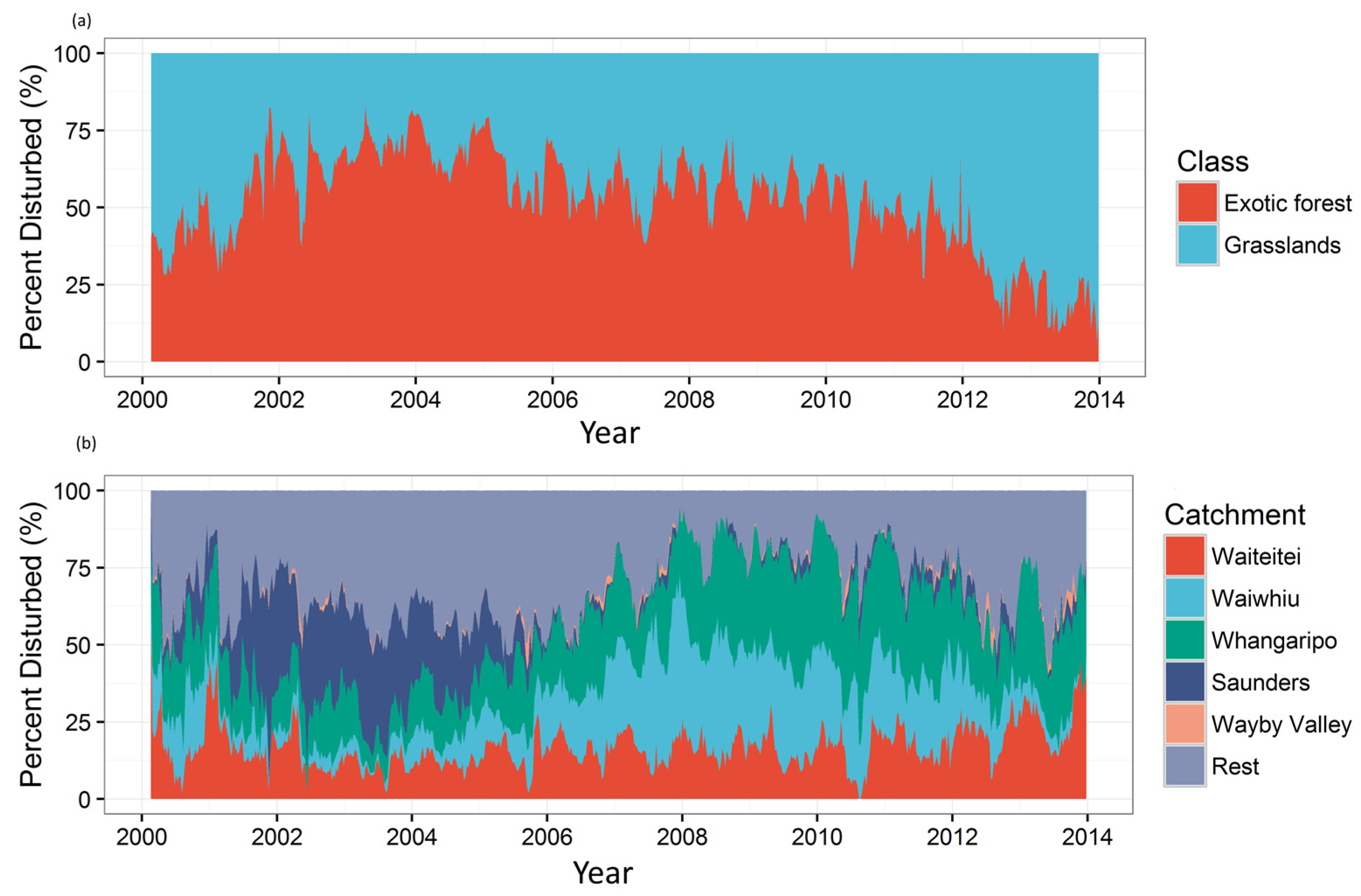
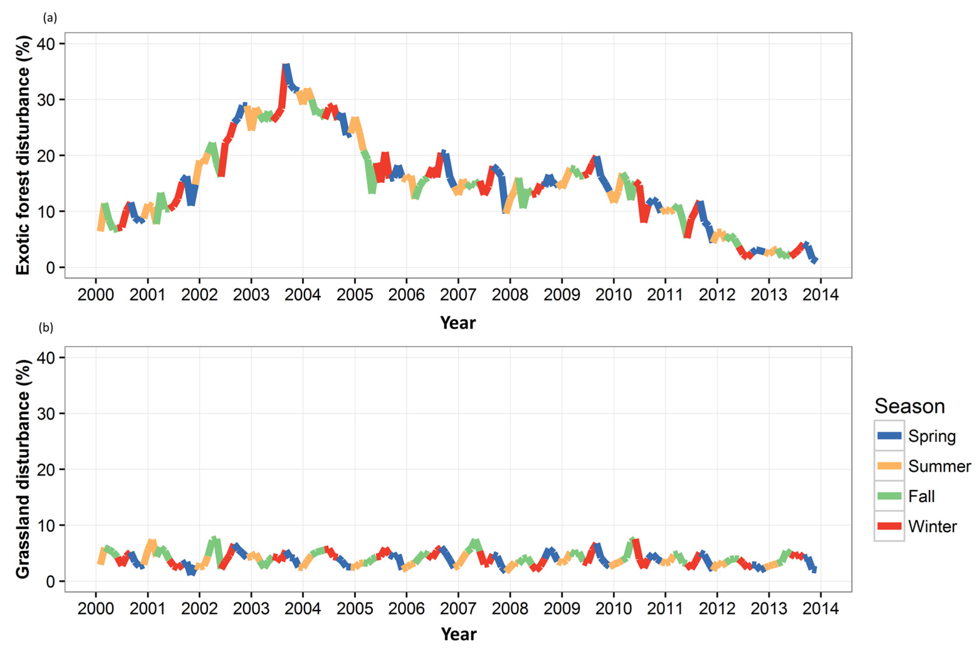
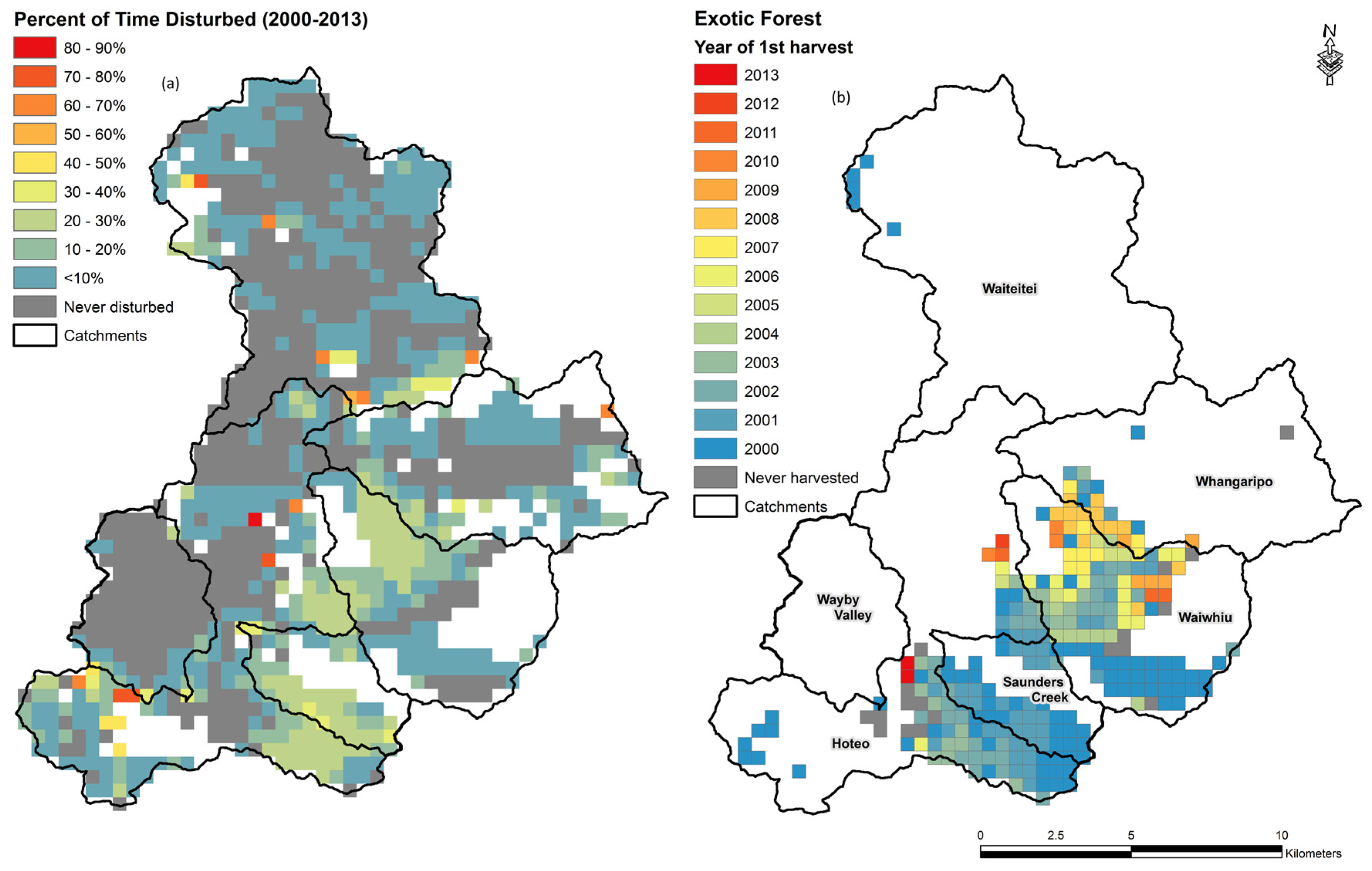
3.1. Land Use and Disturbance at the Sub-Catchment Scale

The spatial distribution of disturbances among high-producing grasslands and exotic forests was variable across the catchment (Figure 2a). Individual pixels were disturbed from 0–83% of the time. Moderate-to-high disturbance frequency (yellow-orange color) was found in Waiwhiu, Whangaripo, and Saunders, as well as near the Hoteo watershed outlet. Some very disturbed pixels (red color) were spread across the watershed, and are results of areas with mixed land cover (e.g., human structures like houses and roads in grassland pixels). By deriving the time of harvest of the exotic forests (Figure 2b), we found that most of the harvesting occurred from 2000–2004 (blue-green color), with 65% of that class being disturbed during the first four years of the record. Most of the exotic forestry was located in Waiwhiu, Saunders, and Whangaripo. The latest harvests occurred along the border of Waiwhiu–Whangaripo. Overall, the percentage of the Hoteo catchment disturbed ranged from 2.0%–13.7% at any given time with a mean of 7.3% for the 2000–2013 period.
The relative contribution to disturbance by land cover also varied over our study period (Figure 3a). Exotic forestry contributed most of the observed land disturbance from 2000–2010 and decreased significantly after 2012. In general, exotic forests were more disturbed, with a mean of 14.9% of the class being disturbed (max of 38% at 14 September 2003 and min of 0.4% on 19 December 2013). Grasslands were less disturbed with a mean of 4% (max of 11.2% at 1 May 2002 and min of 0.7% on 17 November 2001).
Sub-catchment contributions to overall DI formed 2 distinct groups (Figure 3b). Forested catchments such as Waiwhiu and Saunders displayed periods of high disturbance (harvest phase) followed by periods of low disturbance (recovery phase) and appear to be more disturbed (maximum values of 23.4% and 72.2%) at any given time. Pasture-dominated catchments such as Waiteitei and Wayby Valley, on the other hand, displayed a more seasonal pattern and appear less disturbed (maximum values of 17.9% and 13.9%) for a shorter time period (means of 3.9% and 1%). Whangaripo—with a 2-to-1 grassland-to-forest ratio—appears significantly disturbed with a max of 27% and a mean of 9.7%.

3.2. Landscape Connectivity

From the landscape connectivity model (Figure 4), 32% of Hoteo’s catchment was not connected to its stream channels, while 68% was connected either through hillslope runoff (54%) or adjacent floodplain (14%). Most of the connected areas were on the hilly uplands (Whangaripo, Waiwhiu, and Saunders), while the disconnected areas were located on the flat grasslands (Waiteitei and Wayby Valley). More specifically, the percentage of connected areas for each sub-catchment were: Waiteitei 49.6%, Whangaripo 78.4%, Waiwhiu 95.7%, Wayby Valley 45.6%, and Saunders 93.7%. Exotic forests were almost exclusively situated on areas of high elevation/steep slope and thus were more connected than grasslands (79% and 40.4%, respectively).

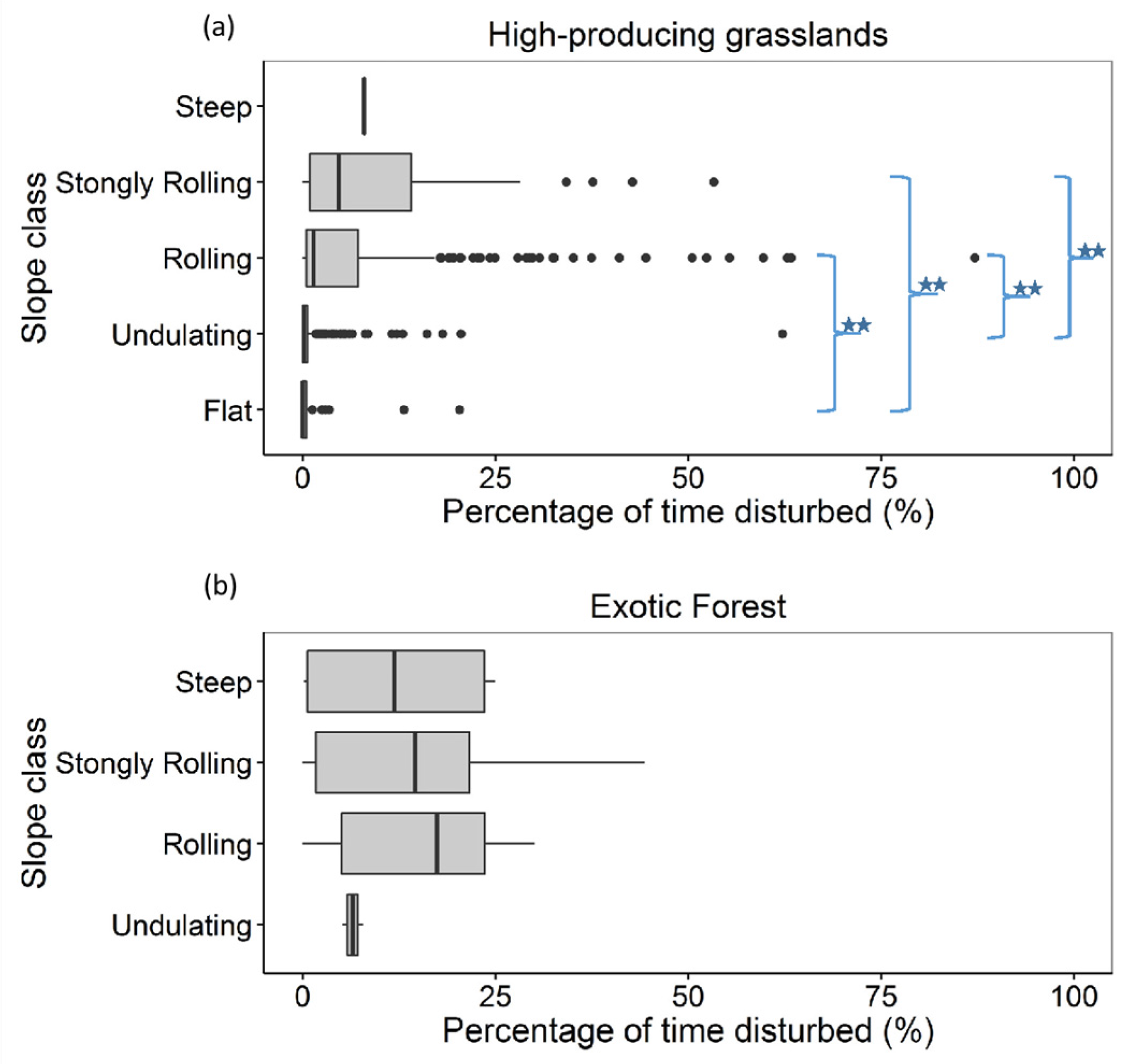
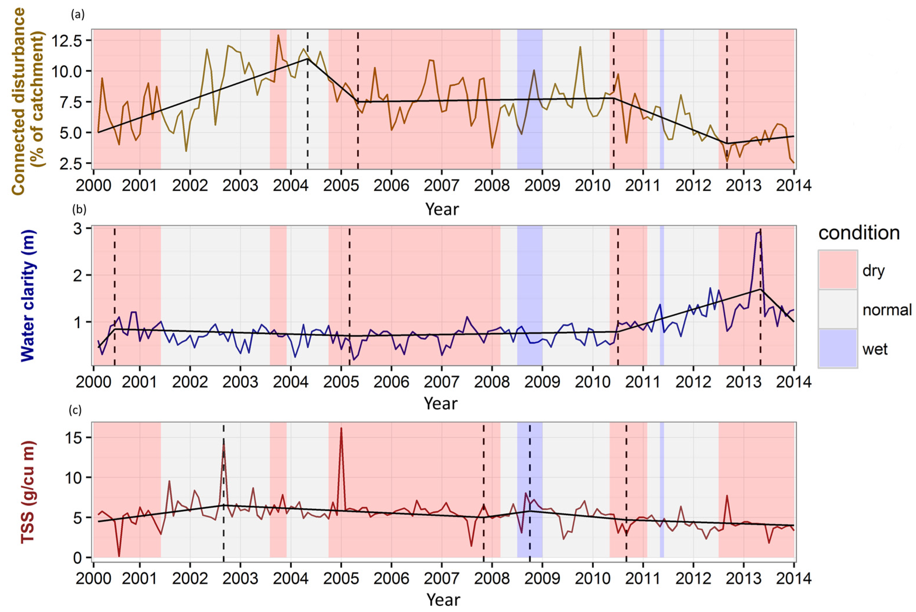
3.3. Physiographic and Hydrologic Effects on Land Disturbance

Results of pairwise comparison using the Wilcoxon rank sum test with the Bonferroni correction showed that areas with exotic forestry had significantly more disturbance than high-producing grasslands (p < 0.001). Steep slopes (≥8°) overall (including both grass and forest) had significantly higher disturbance than gentle slopes (0–8°; p < 0.001). Grasslands on steep slopes also had higher disturbance compared to grasslands on gentle slopes (p-value < 0.001; Figure 5).
There was not much variation in soil type across the catchment. Except for the recent soils in the alluvial floodplain, the vast majority of the catchment was composed of Ultic soils, which are strongly weathered, well-structured clayey soils. Accordingly, they have moderate-high soil moisture, but are poor-draining and susceptible to erosion. Forested areas were dominated by clay loams, whereas pastures had a mix of clay/clay loams.
The connection of long-term precipitation patterns was shown on the SPI vs. monthly connected disturbance time-series (Figure 6a). Drought occurs when SPI falls below −1 and continues until SPI becomes positive. The timing of DI breakpoints coincided with the occurrence of extended periods of drought; more specifically in 2005, 2010, and 2013, the latter being the most severe drought for Hoteo on record.
The percentage of grasslands disturbed varied seasonally, with typically higher values during Winter/Spring and lower during Summer/Fall (Figure 7). Exceptions occurred during extended droughts (2000–2001, 2005–2008, 2010, and 2013), when disturbance was highest during Summer/Fall. Exotic forests exhibited similar seasonal behavior, but disturbance increases or decreases (Figure 6) were mostly influenced by forest harvests (Figure 3b) or recovery, respectively—especially during the 2002–2005 period.

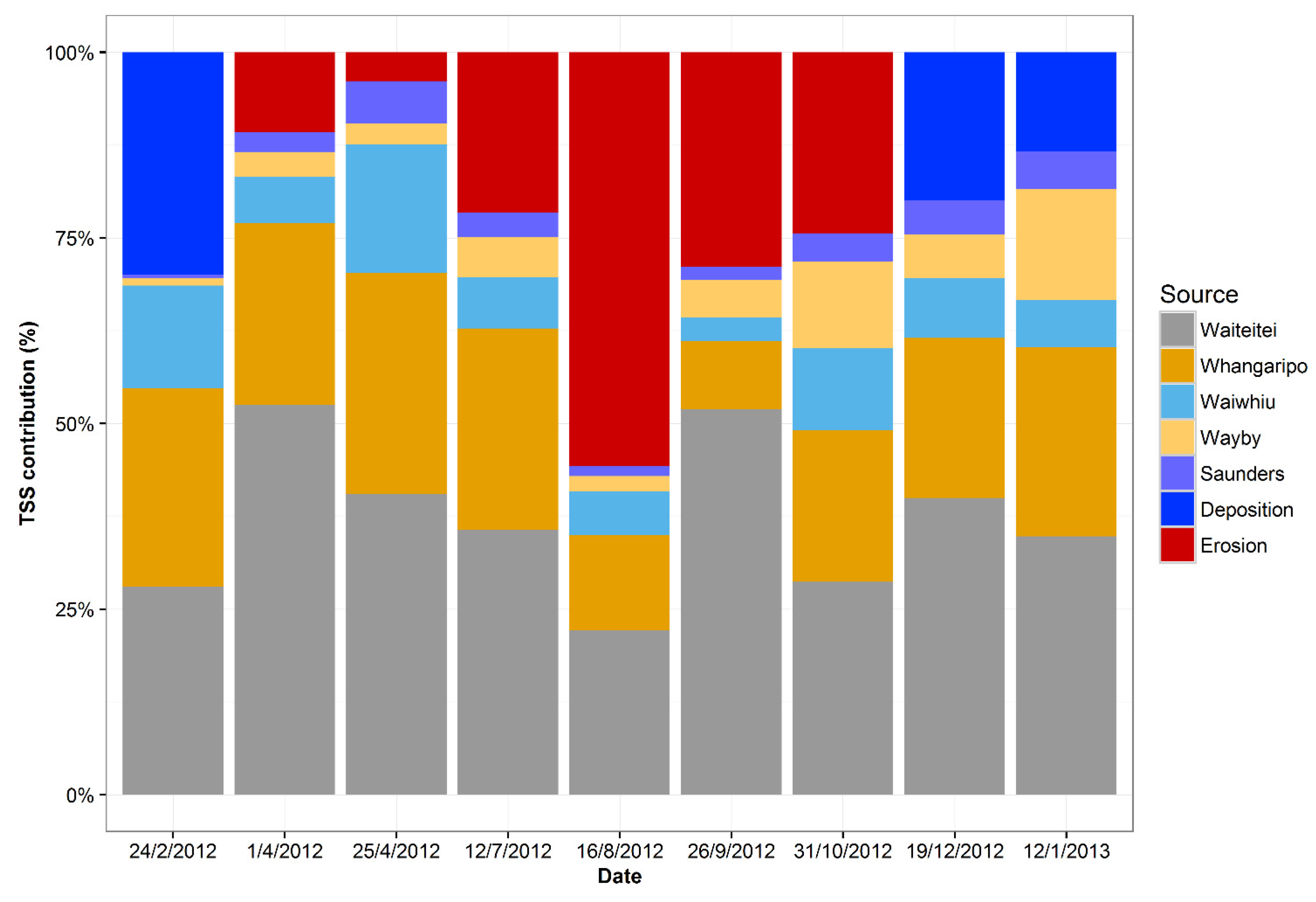
3.4. TSS Spatiotemporal Dynamics

The connected disturbance vs. flow-adjusted clarity time-series had a stronger relationship than connected disturbance vs. TSS (Figure 6). A piecewise regression analysis [57,58] was performed to identify the breakpoints of change in the trend on this set of time series. The regression breakpoints occurred at approximately the same time (2005, 2010, and 2013) for both connected disturbance and water clarity, with diverging trends. The piecewise regression for water clarity had an R2 of 0.55, while the connected disturbance regression had an R2 of 0.59. Breakpoints for TSS did not line up with breakpoints for connected disturbance and water clarity during 2002, 2007, and 2008, but did in 2010. Note that the regression fit for TSS was relatively weak, with an R2 of 0.26. All breakpoints and standard errors are summarized in Table 3.
When relative contributions of TSS by sub-catchment for a relatively normal year in terms of precipitation (2012) were analyzed, an interesting pattern emerged (Figure 8). Net loss erosion (more sediment coming from the main channel or lower catchment than delivered by the sub-catchments) occurred during the Winter (July–October), while net storage deposition (more sediment coming out of the sub-catchments than delivered to the catchment outlet) occurred during the Summer (December–February).
Ranking sub-catchments by their mean TSS daily loads resulted in Waiteitei (2.4 t/d) being the largest contributor, followed by Whangaripo (1.7 t/d), Waiwhiu (0.8 t/d), Wayby Valley (0.2 t/d), and Saunders (0.1 t/d). However, when normalized by area and expressed as specific sediment yields, Whangaripo ranked first, with 3.7 × 10⁻⁴ t/ha/d, followed by Waiteitei (3 × 10⁻⁴ t/ha/d), Waiwhiu (2.1 × 10⁻⁴ t/ha/d), Wayby Valley (0.9 × 10⁻⁴ t/ha/d), and Saunders (0.8 × 10⁻⁴ t/ha/d).
Event-scale TSS data at the Hoteo catchment outlet from 2012–2014 (via a continuously monitoring turbidity sensor) showed a distinct nonlinear pattern (Figure 9) where relative TSS (via LOESS residuals) declined after sediment-laden floods, but eventually recovered and increased until the next large flood. This sine-like wave with sediment pulses (peaks) and sediment exhaustion (troughs) had almost four cycles over this 3 year period.

4. Discussion

4.1. Connections among Land Use, Climate, Disturbance, and Sediment Runoff

While many studies have investigated sediment runoff effects of land uses such as forest harvesting [57,58] and livestock grazing [59,60] at the catchment scale over coarse time-scales, here we examined the more direct link to sediment runoff of connected disturbance (with 8 day resolution) at the sub-catchment scale. When comparing land use, connected disturbance, and sediment runoff, a clear pattern emerged: plantation forest areas were significantly more disturbed and more connected than high-producing grasslands, with correspondingly high TSS loads. Whangaripo and Waiwhiu contributed most of the landscape disturbance (Figure 2a), with an average of 23.5% and 17.2%, due to forest clearings on the area along their border that mainly occurred after 2006 (Figure 2b). They also both ranked very high on TSS, being the 1st and 3rd sediment runoff contributors in terms of t/year. Saunders was almost completely cleared during 2000–2002 (Figure 2b), an area that has since been reforested and now has relatively low specific sediment yields. On the contrary, Waiteitei, which is 94% pasture, consistently contributes 16.7% of the disturbance, on average, along with having the 2nd-highest specific sediment yield. Lastly, Wayby Valley (which is 97% pasture land) contributes only 0.7% of the disturbance on average with very low specific sediment yields. In summary, different land uses in the Hoteo catchment produced varying amounts of available sediment, and when land disturbance changed (from forest harvests, droughts, and possibly over-grazing), the magnitude and timing of sediment delivery to rivers also changed.
Climate and land cover are intricately connected with both positive and negative feedbacks affecting their relationship [15,61]. Extended periods of drought are expected to have a detrimental effect on vegetation, with significant vegetation die-off and increased areas of exposed soil [62]. This would result in an increase in land disturbance (measured as connected disturbance in this study) unless mitigated by management responses such as fertilization, irrigation, supplemental feed, and reduced grazing. While we were not able to thoroughly assess all of these management practices across the entire catchment, numerous field observations and discussions with local farmers indicate that some of these practices were occurring at various times in our study period. However, management intensity in this region is relatively minor compared to other parts of New Zealand [63], and thus most of the land–water relationships we observed were likely from biophysical processes. The main exception was plantation forest harvests. The connected disturbance increased up to 2004 can mostly be explained by forest clearings over relatively steep areas of the catchment (Figure 2, Figure 3, and Figure 6), especially Waiwhiu, Saunders, and Whangaripo. The drought—which began in late in 2004 and lasted until the start of 2008—kept land disturbance at moderate levels (Figure 6a), with 7.6% of the catchment being disturbed on average. Further, in January 2013, disturbed area doubled in response to a severe drought, which in turn led to a sharp decrease in water clarity (Figure 6a,b).

4.2. Landscape–River Connectivity

Determining landscape–river connectivity is crucial in the evaluation of whether land use changes have the potential to affect river water quality. Since the broad-scale European settlement of New Zealand, landscape connectivity has increased with the clearings of native vegetation, the addition of millions of sheep and cattle, and the consequent channel erosion and extensive gully formation [64]. The landscape connectivity model developed here is similar to the Highly Erodible Land (HEL) model [65] which used the largely perennial REC stream network. In order to advance this model and concept, we mapped the intermittent and ephemeral channels and thus accounted for the higher degree of connectivity present on the landscape. Given that most of a catchment’s sediment yield occurs during large storms [66,67,68] when ephemeral channels are active, it is important to account for these connected channels.
A more representative channel network map and a corresponding connectivity dataset is also useful for the identification and prioritization of sites for best management practices (BMPs) that improve water quality. Vegetation buffers, in particular, have been shown to filter sediment, nutrient, and other pollutant runoff before entering streams [69,70,71]; however, there is no consensus on the most effective location or size of these vegetation buffers [72]. Our connectivity map and land disturbance analyses could provide insight on ideal buffer placement, which would be between stream channels and connected areas that are frequently disturbed (Figure 2 and Figure 4). The size of these vegetation buffers could be determined based on contributing drainage area, slope, and amount of connected disturbance. Properly characterizing land disturbance and its connectivity to stream channels at the catchment scale is important for siting other BMPs, such as rain gardens and detention/retention ponds [73].

4.3. Nonlinear Changes

Using multiple resolutions of data at multiple scales, we found clear nonlinear changes in land disturbance, climate, and consequently sediment runoff (Figure 3, Figure 6, Figure 8 and Figure 9). The nonlinear patterns in TSS and water clarity appear to be the combined result of: (1) high sediment loadings to rivers from connected disturbed areas, which change in location and extent over time (Figure 2 and Figure 3); (2) sediment supply limitation following sediment-laden floods (Figure 9); and (3) shifts between erosion and deposition in the channels (Figure 8). From several years of observation by us and others [42], there are large stores of sediment along the mainstem Hoteo River, which change from flood to flood. While it is this in-channel sediment that makes the Hoteo River one of the most turbid rivers in all of New Zealand [63], this sediment has been derived from major landscape disturbances over the past 150 years [42]. These legacy effects also contribute to nonlinear changes in water quality and a level of complexity that was beyond the temporal scope of this study.
For the assessment of nonlinear water quality trends, the disturbance index (DI) demonstrated the potential to be a water quality indicator. The breakpoint analyses (Figure 6) showed that significant changes/trends of connected disturbance and water clarity coincide, suggesting a cause-and-effect relationship between them on the temporal dimension. TSS time-series showed weak connection with connected disturbance; however, suspended sediment budgets were very useful for connecting sediment runoff to specific sub-catchments on the space dimension. The suspended sediment budgets also provided insight on depositional/erosional processes in the river channel/floodplain (Figure 8). For the latter, it is very important to consider the value of riparian fencing that can greatly affect these erosional/depositional process along the channel. While some of the perennial channels on dairy farms (a small percentage of the drainage network) were fenced, the majority of the intermittent and ephemeral tributaries were unfenced, and thus are likely to be significantly contributing to sediment runoff during high-flow events.
The location and timing of forest harvests, coupled with TSS/water clarity data suggest that exotic forestry is the major contributor of disturbance and sediment to the rivers. On average, exotic forests are more disturbed than grasslands (18 months vs 3.8 months) [10], because the latter recover much faster. Connected disturbance increased significantly during the 2000–2004 period, where 65% of the forests in the Hoteo catchment were harvested. On the contrary, suspended sediment samples taken from all sub-catchments suggest that during periods of low disturbance (2012–2013), pasture watersheds contribute more sediment—anywhere from 25%–50% of the total suspended sediment measured. Over the course of seasons (Figure 8 and Figure 9) and years (Figure 3, Figure 6, and Figure 7), all of these cross-scale interactions among land cover/use, climate, and land disturbance (over both space and time) described throughout this Discussion have produced unique nonlinear patterns in sediment runoff that need to be explored further.

5. Conclusions

The purpose of this study was to assess nonlinear LCLUC–water quality relationships and locate the sources of sediment runoff across the Hoteo catchment in New Zealand. Suspended sediment budget analyses showed that exotic forests were the dominant sediment source in periods of forest harvesting, while grasslands assumed the dominant role once exotic forests recover. Further analyses showed that connected land disturbance and water clarity time-series exhibited similar breakpoints on their trends, suggesting a cause-and-effect relationship. When the sequence of flood events was assessed, these changes in supply and transport of sediment resulted in a cyclical pattern of sediment runoff. Future investigations on water quality changes would benefit from an assessment of connected land disturbance. It has definitely been a useful water quality indicator in this study, especially when combined with climate data. The connectivity layer developed here could also serve as a guide to place and prioritize BMPs, especially in the form of vegetation buffers to reduce sediment runoff into rivers. Reducing suspended sediment in impacted rivers such as the Hoteo would further benefit downstream receiving waters with sedimentation or water quality problems. Indeed, the Kaipara Harbour (in which the Hoteo River drains) is a valuable and sensitive estuarine ecosystem that is experiencing considerable sediment infilling and associated environmental degradation. The focus of this study was seasonal and yearly changes in sediment runoff. The next step in this line of research would be to investigate the changes and relationships among land cover/use, climate, land disturbance, and other water quality variables at even finer spatiotemporal scales over longer periods.

Acknowledgments

Julian and de Beurs (Co-PIs) were funded by NASA LCLUC grant NNX14AB77G and NSF Geography grants #1359970 and #1359948. Julian was also funded by a Fulbright Senior Scholar Fellowship, which was hosted by the National Institute of Water & Atmospheric Research (NIWA) in Hamilton, NZ. Hughes was funded by NIWAs Management of Cumulative Effects of Stressors on Aquatic Ecosystems Research Programme (MBiE Contract: CO1X1005). Auckland Council provided flow and continuous turbidity data. Thanks to Hugh and Anthea McKergow for accommodation during site visits.

Author Contributions

Julian, Kamarinas, and Hughes designed the study. Kamarinas performed most of the analyses. Julian and Hughes collected and analyzed field data. de Beurs and Owsley developed the disturbance dataset. Kamarinas prepared the manuscript with contributions from all co-authors.

Conflicts of Interest

The authors declare no conflict of interest.

References

  1. Foley, J.A.; DeFries, R.; Asner, G.P.; Barford, C.; Bonan, G.; Carpenter, S.R.; Chapin, F.S.; Coe, M.T.; Daily, G.C.; Gibbs, H.K.; et al. Global consequences of land use. Science 2005, 309, 570–574. [Google Scholar] [CrossRef] [PubMed]
  2. Vitousek, P.M.; Mooney, H.A.; Lubchenco, J.; Melillo, J.M. Human domination of Earth’s ecosystems. Science 1997, 277, 494–499. [Google Scholar] [CrossRef]
  3. Allan, J.D. Landscapes and riverscapes: The influence of land use on stream ecosystems. Annu. Rev. Ecol. Evol. Syst. 2004, 35, 257–284. [Google Scholar] [CrossRef]
  4. Tong, S.T.Y.; Chen, W. Modeling the relationship between land use and surface water quality. J. Environ. Manag. 2002, 66, 377–393. [Google Scholar] [CrossRef]
  5. Phillips, J.D. Sources of nonlinearity and complexity in geomorphic systems. Progress Phys. Geogr. 2003, 27, 1–23. [Google Scholar] [CrossRef]
  6. Quinn, J.M.; Cooper, A.B.; Davies-Colley, R.J.; Rutherford, J.C.; Williamson, R.B. Land use effects on habitat, water quality, periphyton, and benthic invertebrates in Waikato, New Zealand, hill-country streams. N. Z. J. Mar. Freshw. Res. 1997, 31, 579–597. [Google Scholar] [CrossRef]
  7. Schilling, K.E.; Isenhart, T.M.; Palmer, J.A.; Wolter, C.F.; Spooner, J. Impacts of land-cover change on suspended sediment transport in two agricultural watersheds. J. Am. Water Res. Assoc. 2011, 47, 672–686. [Google Scholar] [CrossRef]
  8. New Zealand Land Cover Database; Landcare Research (LCR): Lincoln, New Zealand, 2015.
  9. Homer, C.; Dewitz, J.; Yang, L.; Jin, S.; Danielson, P.; Xian, G.; Coulston, J.; Herold, N.; Wickham, J.; Megown, K. Completion of the 2011 national land cover database for the conterminous United States—Representing a decade of land cover change information. Photogr. Eng. Remote Sens. 2015, 81, 345–354. [Google Scholar]
  10. De Beurs, K.M.; Owsley, B.C.; Julian, J.P. Disturbance analyses of forests and grasslands with MODIS and Landsat in New Zealand. Inter. J. Appl. Earth Obs. Geoinfor. 2016, 45, 42–54. [Google Scholar] [CrossRef]
  11. Lambin, E.F.; Rounsevell, M.D.A.; Geist, H.J. Are agricultural land-use models able to predict changes in land-use intensity? Agric. Ecosyst. Environ. 2000, 82, 321–331. [Google Scholar] [CrossRef]
  12. Julian, J.P.; Davies-Colley, R.J.; Gallegos, C.L.; Tran, T.V. Optical water quality of inland waters: A landscape perspective. Ann. Assoc. Am. Geogr. 2013, 103, 309–318. [Google Scholar] [CrossRef]
  13. Abbaspour, K.C.; Yang, J.; Maximov, I.; Siber, R.; Bogner, K.; Mieleitner, J.; Zobrist, J.; Srinivasan, R. Modelling hydrology and water quality in the pre-alpine/alpine Thur watershed using SWAT. J. Hydrol. 2007, 333, 413–430. [Google Scholar] [CrossRef]
  14. Hunter, H.M.; Walton, R.S. Land-use effects on fluxes of suspended sediment, nitrogen and phosphorus from a river catchment of the great barrier reef, Australia. J. Hydrol. 2008, 356, 131–146. [Google Scholar] [CrossRef]
  15. Knox, J.C. Valley alluviation in southwestern Wisconsin. Ann. Assoc. Am. Geogr. 1972, 62, 401–410. [Google Scholar] [CrossRef]
  16. Milliman, J.D.; Syvitski, J.P.M. Geomorphic/tectonic control of sediment discharge to the ocean: The importance of small mountainous rivers. J. Geol. 1992, 100, 525–544. [Google Scholar] [CrossRef]
  17. Croke, J.C.; Hairsine, P.B. Sediment delivery in managed forests: A review. Environ. Rev. 2006, 14, 59–87. [Google Scholar] [CrossRef]
  18. Kreutzweiser, D.P.; Capell, S.S. Fine sediment deposition in streams after selective forest harvesting without riparian buffers. Can. J. For. Res. 2001, 31, 2134–2142. [Google Scholar] [CrossRef]
  19. Neal, C.; Reynolds, B.; Wilkinson, J.; Hill, T.; Neal, M.; Hill, S.; Harrow, M. The impacts of conifer harvesting on runoff water quality: A regional survey for Wales. Hydrol. Earth Sys. Sci. 1998, 2, 323–344. [Google Scholar] [CrossRef]
  20. Fahey, B.; Marden, M.; Phillips, C. Sediment yields from plantation forestry and pastoral farming, coastal Hawke’s Bay, North Island, New Zealand. J. Hydrol. 2003, 42, 27–38. [Google Scholar]
  21. Fransen, P.J.B.; Phillips, C.J.; Fahey, B.D. Forest road erosion in New Zealand: Overview. Earth Surf. Process. Landf. 2001, 26, 165–174. [Google Scholar] [CrossRef]
  22. Motha, J.A.; Wallbrink, P.J.; Hairsine, P.B.; Grayson, R.B. Determining the sources of suspended sediment in a forested catchment in southeastern Australia. Water Resour. Res. 2003, 39, 1056–1069. [Google Scholar] [CrossRef]
  23. Bartley, R.; Corfield, J.P.; Abbott, B.N.; Hawdon, A.A.; Wilkinson, S.N.; Nelson, B. Impacts of improved grazing land management on sediment yields, part 1: Hillslope processes. J. Hydrol. 2010, 389, 237–248. [Google Scholar] [CrossRef]
  24. Daniel, J.A.; Phillips, W.A.; Northup, B.K. Influence of summer management practices of grazed wheat pastures on runoff, sediment, and nutrient losses. Trans. ASABE 2006, 49, 349–355. [Google Scholar] [CrossRef]
  25. Quinn, J.M.; Stroud, M.J. Water quality and sediment and nutrient export from New Zealand hill-land catchments of contrasting land use. N. Z. J. Mar Freshw. Res. 2002, 36, 409–429. [Google Scholar] [CrossRef]
  26. McDowell, R.W. Grazed Pastures and Surface Water Quality; Nova Science Publishers: New York, NY, USA, 2008. [Google Scholar]
  27. Peters, D.C.; Bestelmeyer, B.; Turner, M. Cross-scale interactions and changing pattern-process relationships: Consequences for system dynamics. Ecosystems 2007, 10, 790–796. [Google Scholar] [CrossRef]
  28. Marston, R.A. Geomorphology and vegetation on hillslopes: Interactions, dependencies, and feedback loops. Geomorphology 2010, 116, 206–217. [Google Scholar] [CrossRef]
  29. Wischmeier, W.H.; Mannering, J.V. Relation of soil properties to its erodibility. Soil Sci. Soc. Am. J. 1969, 33, 131–137. [Google Scholar] [CrossRef]
  30. Elmore, A.J.; Julian, J.P.; Guinn, S.M.; Fitzpatrick, M.C. Potential stream density in mid-Atlantic U.S. Watersheds. PLoS ONE 2013, 8, e74819. [Google Scholar] [CrossRef] [PubMed]
  31. Montgomery, D.R.; Dietrich, W.E. Channel initiation and the problem of landscape scale. Science 1992, 255, 826–830. [Google Scholar] [CrossRef] [PubMed]
  32. Wohl, E. Rivers in the Landscape; WILEY Blackwell: Chichester, UK, 2014; p. 318. [Google Scholar]
  33. Julian, J.P.; Elmore, A.J.; Guinn, S.M. Channel head locations in forested watersheds across the mid-Atlantic united states: A physiographic analysis. Geomorphology 2012, 177–178, 194–203. [Google Scholar] [CrossRef]
  34. Gergel, S.E.; Turner, M.G.; Miller, J.R.; Melack, J.M.; Stanley, E.H. Landscape indicators of human impacts to riverine systems. Aquat. Sci. 2002, 64, 118–128. [Google Scholar] [CrossRef]
  35. Borselli, L.; Cassi, P.; Torri, D. Prolegomena to sediment and flow connectivity in the landscape: A GIS and field numerical assessment. Catena 2008, 75, 268–277. [Google Scholar] [CrossRef]
  36. Bracken, L.J.; Croke, J. The concept of hydrological connectivity and its contribution to understanding runoff-dominated geomorphic systems. Hydrol. Process. 2007, 21, 1749–1763. [Google Scholar] [CrossRef]
  37. Bracken, L.J.; Turnbull, L.; Wainwright, J.; Bogaart, P. Sediment connectivity: A framework for understanding sediment transfer at multiple scales. Earth Surf. Process. Landf. 2015, 40, 177–188. [Google Scholar] [CrossRef] [Green Version]
  38. Palmer, D.; Dymond, J.; Basher, L. Assessing Erosion in the Waipa Catchment Using the New Zealand Empirical Erosion Model (NZEEM®), Highly Erodible Land (HEL), and SedNetNZ Models; Landcare Research: Lincoln, New Zealand, 2013; p. 31. [Google Scholar]
  39. Uriarte, M.; Yackulic, C.B.; Lim, Y.; Arce-Nazario, J.A. Influence of land use on water quality in a tropical landscape: A multi-scale analysis. Landsc. Ecol. 2011, 26, 1151–1164. [Google Scholar] [CrossRef] [PubMed]
  40. Fryirs, K.A.; Brierley, G.J.; Preston, N.J.; Kasai, M. Buffers, barriers and blankets: The (dis)connectivity of catchment-scale sediment cascades. Catena 2007, 70, 49–67. [Google Scholar] [CrossRef]
  41. Walling, D.E. Scale problems in hydrology the sediment delivery problem. J. Hydrol. 1983, 65, 209–237. [Google Scholar] [CrossRef]
  42. Buikema, R. A Conceptualisation of Strategic Riparian Management Using Geomorphology and Spatio-Temporal Analysis: Hoteo River Catchment, Auckland. Master’s Thesis, The University of Auckland, Auckland, New Zealand, 2012. [Google Scholar]
  43. Lobser, S.; Cohen, W. MODIS tasselled cap: Land cover characteristics expressed through transformed MODIS data. Int. J. Remote Sens. 2007, 28, 5079–5101. [Google Scholar] [CrossRef]
  44. Webb, T.H.; Wilson, A.D. A Manual of Land Characteristics for Evaluation of Rural Land; Manaaki Whenua Press: Lincoln, New Zealand, 1995. [Google Scholar]
  45. Snelder, T.H.; Biggs, B.J.F.; Weatherhead, M. New Zealand River Environment Classification User Guide; National Institute of Water and Atmospheric Research: Wellington, New Zealand, 2004. [Google Scholar]
  46. Davies-Colley, R.J.; Smith, D.G.; Ward, R.C.; Bryers, G.G.; McBride, G.B.; Quinn, J.M.; Scarsbrook, M.R. Twenty years of new Zealand’s national rivers water quality network: Benefits of careful design and consistent operation. J. Am. Water Resour. Assoc. 2011, 47, 750–771. [Google Scholar] [CrossRef]
  47. Ballantine, D.; Hughes, A.; Davies-Colley, R. Mutual relationships of suspended sediment, turbidity and visual clarity in New Zealand rivers. Proc. IAHS 2015, 367, 265–271. [Google Scholar] [CrossRef]
  48. Gray, J.R.; Simões, F.J.M. Estimating sediment discharge. In Sedimentation Engineering; American Society of Civil Engineering Manuals and Reports on Engineering Practice: Reston, VA, USA, 2008; pp. 1067–1088. [Google Scholar]
  49. Hughes, A.; Davies-Colley, R.; Elliott, A. Measurement of light attenuation extends the application of suspended sediment monitoring in rivers. In Proceedings of the International Association of Hydrological Sciences, New Orleans, LA, USA, 11–14 December 2014; IAHS: New Orleans, LA, USA, 2014; Volume 367, pp. 170–176. [Google Scholar]
  50. Cleveland, W.S.; Devlin, S.J. Locally weighted regression: An approach to regression analysis by local fitting. J. Am. Stat. Assoc. 1988, 83, 596–610. [Google Scholar] [CrossRef]
  51. Eaton, A.D.; Franson, M.A.H. Standard Methods for the Examination of Water & Wastewater; American Public Health Association; American Water Works Association; Water Environment Federation: Washington, DC, USA, 2005. [Google Scholar]
  52. Moore, R.D.; Spittlehouse, D.L.; Story, A. Riparian microclimate and stream temperature response to forest harvesting: A review. J. Am. Water Resour. Assoc. 2005, 41, 813–834. [Google Scholar] [CrossRef]
  53. McKee, T.B.; Doesken, N.J.; Kleist, J. The relationship of drought frequency and duration of time scales. In Proceedings of the 8th Conference on Applied Climatology, Anaheim, CA, USA, 17–22 January 1993; American Meteorological Society: Anaheim, CA, USA, 1993; pp. 179–186. [Google Scholar]
  54. World Meteorological Organization. Standardized Precipitation Index User Guide; Svoboda, M., Hayes, M., Wood, D., Eds.; WMO-No. 1090; WHO: Geneva, Switzerland, 2012. [Google Scholar]
  55. Muggeo, V.M.R. Segmented: An R package to fit regression models with broken-line relationships. R News 2008, 8, 20–25. [Google Scholar]
  56. Lynn, I.; Manderson, A.; Page, M.; Harmsworth, G.; Eyles, G.; Douglas, G.; Mackay, A.; Newsome, P. Updating and Producing the Land Use Capability Survey Handbook, 3rd ed.; Landcare Research: Lincoln, New Zealand, 2009; p. 163. [Google Scholar]
  57. Arthur, M.A.; Coltharp, G.B.; Brown, D.L. Effects of best management practices on forest streamwater quality in eastern Kentucky. J. Am. Water Resour. Assoc. 1998, 34, 481–495. [Google Scholar] [CrossRef]
  58. Swank, W.T.; Vose, J.M.; Elliott, K.J. Long-term hydrologic and water quality responses following commercial clearcutting of mixed hardwoods on a southern Appalachian catchment. Forest Ecol. Manag. 2001, 143, 163–178. [Google Scholar] [CrossRef]
  59. McDowell, R.W. Phosphorus and sediment loss in a catchment with winter forage grazing off cropland by dairy cattle. J. Environ. Qual. 2006, 35, 575–583. [Google Scholar] [CrossRef] [PubMed]
  60. Monaghan, R.M.; Wilcock, R.J.; Smith, L.C.; Tikkisetty, B.; Thorrold, B.S.; Costall, D. Linkages between land management activities and water quality in an intensively farmed catchment in southern New Zealand. Agric. Ecosys. Environ. 2007, 118, 211–222. [Google Scholar] [CrossRef]
  61. Bonan, G.B. Forests and climate change: Forcings, feedbacks, and the climate benefits of forests. Science 2008, 320, 1444–1449. [Google Scholar] [CrossRef] [PubMed]
  62. Anderegg, W.R.L.; Kane, J.M.; Anderegg, L.D.L. Consequences of widespread tree mortality triggered by drought and temperature stress. Nature Clim. Change 2013, 3, 30–36. [Google Scholar] [CrossRef]
  63. Julian, J.P.; de Beurs, K.M.; Owsley, B.; Davies-Colley, R.J.; Ausseil, A.G.E. River water quality changes in New Zealand over 26 years (1989–2014): Response to land use and land disturbance. Hydrol. Earth Syst. Sci. Discuss. 2016, 2016, 1–69. [Google Scholar] [CrossRef]
  64. Glade, T. Landslide occurrence as a response to land use change: A review of evidence from New Zealand. Catena 2003, 51, 297–314. [Google Scholar] [CrossRef]
  65. Dymond, J.R.; Ausseil, A.-G.; Shepherd, J.D.; Buettner, L. Validation of a region-wide model of landslide susceptibility in the Manawatu–Wanganui region of New Zealand. Geomorphology 2006, 74, 70–79. [Google Scholar] [CrossRef]
  66. Basher, L.R.; Hicks, D.M.; Clapp, B.; Hewitt, T. Sediment yield response to large storm events and forest harvesting, Motueka River, New Zealand. N. Z. J. Mar. Fres. Res. 2011, 45, 333–356. [Google Scholar] [CrossRef]
  67. Milliman, J.D.; Meade, R.H. World-wide delivery of river sediment to the oceans. J. Geol. 1983, 91, 1–21. [Google Scholar] [CrossRef]
  68. Reid, L.; Page, M. Magnitude and frequency of landsliding in a large New Zealand catchment. Geomorphology 2003, 49, 71–88. [Google Scholar] [CrossRef]
  69. Dosskey, M.G.; Eisenhauer, D.E.; Helmers, M.J. Establishing conservation buffers using precision information. J. Soil Water Conserv. 2005, 60, 349–354. [Google Scholar]
  70. Lee, K.H.; Isenhart, T.M.; Schultz, R.C. Sediment and nutrient removal in an established multi-species riparian buffer. J. Soil Water Conserv. 2003, 58, 1–8. [Google Scholar]
  71. Lowrance, R.; Altier, L.S.; Newbold, J.D.; Schnabel, R.R.; Groffman, P.M.; Denver, J.M.; Correll, D.L.; Gilliam, J.W.; Robinson, J.L.; Brinsfield, R.B.; et al. Water quality functions of riparian forest buffers in Chesapeake Bay watersheds. Environ. Manag. 1997, 21, 687–712. [Google Scholar] [CrossRef]
  72. Fischer, R.A.; Fischenich, J.C. Design Recommendations for Riparian Corridors and Vegetated Buffer Strips; DTIC Document: Vicksburg, MS, USA, 2000. [Google Scholar]
  73. Martin-Mikle, C.J.; de Beurs, K.M.; Julian, J.P.; Mayer, P.M. Identifying priority sites for low impact development (LID) in a mixed-use watershed. Landsc. Urban Planning 2015, 140, 29–41. [Google Scholar] [CrossRef]
Figure 1. (a) The Hoteo catchment (located on the North Island, NZ) and its five sub-catchments (black lines) delineated based on the location of gaging stations. Land cover (LCDB v3.3) is shown for reference. Precipitation data were drawn from Warkworth EWS climate station, located 8 km south-east of Hoteo; (b) Climograph created from data drawn from Warkworth EWS climate station for the period 2000–2013.
Water 08 00436 g001
Figure 2. (a) Percent of time of every pixel being disturbed for the 2000–2013 period. White pixels were native forests, which were not assessed for disturbance. (b) The year of first harvest for each one of the exotic forestry pixels. Forests that were not harvested during the study period are shown as grey.
Water 08 00436 g002
Figure 3. (a) Relative contributions of exotic forest (orange) and pasture (blue) to overall watershed disturbance; (b) Disturbance contribution (%) of each sub-catchment relative to the total watershed disturbance.
Water 08 00436 g003
Figure 4. Landscape connectivity for the study area; connected areas (green color) are considered critical source areas of sediment (CSAS) and were used as a mask for land disturbance. A schematic of the rules (as described in Section 2.4) for developing the model are shown on the right side panel. The 1st pixel (upper left corner) is the one being evaluated for connectivity; the next two pixels down the flowpath must both have slope values >5° for the 1st pixel to be considered as connected (green color). If either one of the next two pixels has a slope value <5°, then the pixel being evaluated is considered disconnected (red color). Lastly, if either one of the next two pixels are classified as floodplain, then the pixel is connected (green color).
Water 08 00436 g004
Figure 5. Wilcoxon rank sum test (Bonferroni correction) on disturbance values for different slope (flat, undulating, rolling, strongly rolling, and steep) and land cover classes: (a) high-producing grasslands and (b) exotic forest. Statistical significance between classes is shown with blue stars (p-value < 0.001) on the boxplots.
Water 08 00436 g005
Figure 6. Monthly (a) percentage of catchment connected and disturbed; (b) water clarity (residuals from local polynomial regression (LOESS) + mean clarity; and (c) flow-adjusted TSS (residuals from loess + mean TSS) for the period 2000–2013. The timing of breakpoints (dashed lines) between connected disturbance and water clarity from 2005–2013 seem to coincide, suggesting a cause and effect relationship between the two. Wet (blue), normal (grey), and dry (red) periods were calculated from a 12 month standardized precipitation index (SPI). The segmented regression lines are shown in black.
Water 08 00436 g006
Figure 7. Seasonal variation of disturbance for (a) exotic forestry and (b) high-producing grasslands. Exotic forestry appears to be significantly more disturbed than grasslands from 2000–2010 and even three times more disturbed than grasslands from 2002–2005.
Water 08 00436 g007
Figure 8. Sub-catchment suspended sediment budgets for the 2012–2013 period. Total suspended solids (TSS) contributions were calculated in t/day and are expressed as percentage of total exiting the Hoteo catchment. Net storage (deposition) occurred when the sum of TSS of all sub-catchments exceeded TSS exiting the catchment outlet, while net loss (erosion) occurred when more TSS exited the catchment outlet than was delivered by the sub-catchments.
Water 08 00436 g008
Figure 9. (a) Flow event magnitudes; (b) TSS residuals event (n = 60) analysis from the period 2012–2014 for the Hoteo catchment outlet in order of occurrence showing periods of higher amounts of sediment than expected followed by lower amounts of sediment than expected. The sine-like wave (blue LOESS line with 95% confidence intervals) suggests that after major TSS events (concave), sediment in the landscape is exhausted (convex). Similar patterns were described in Knox’s (1972) [15] seminal paper occurring over thousand years or millennia. Our results show that these processes also take place on yearly or monthly time scales. The date (dd/mm/yyyy) is shown on extreme events.
Water 08 00436 g009
Table 1. Summary of landscape and water quality data used for this research.
DatasetVariable(s)/typeScale, PeriodSource
Disturbance Index (DI)%DI > 3/rasteraMODIS (8-day, 450 m), 2000–2014de Beurs et al., 2016 [10]
Land Cover v3.3Vector polygon1:50,000, 2001–2008Landcare Research
New Zealand Fundamental Soils LayersSilt-clay%/Vector polygon1:50,000, 2000Landcare Research
National Climate DatabaseMonthly precipitation totalsstation, 1922–2014bNIWA
Water quality dataClarity, Turbidity, dTSSMonthly, 2000–2014cNRWQN, bNIWA
dTSSnine monthly samples, 2012–2013Present study
Discharge, Turbidity5 min data, 2011–2014Auckland Council
River Environment Classification v2.0Stream segments/Vector line1:24,000, 2014bNIWA
eDEMElevation/raster15 m, 2012Landcare Research
Auckland 0.5 m rural aerial photosOrtho-photography0.5 m, 2010–2012eLINZ
aModerate Resolution Imaging Spectroradiometer; bNational Institute of Water and Atmospheric Research; cNational River Water Quality Network; dTotal Suspended Solids; eDigital Elevation Model; fLand Information New Zealand.
Table 2. Physiographic characteristics of the study area (Hoteo) and its sub-catchments. Land covers are native forest (NF), exotic forest (EX), high-producing grasslands (HG), and Rest (RE). Landscape connectivity refers to Connected (C), River and floodplain buffer (R), and Disconnected (D).
CatchmentDrainage density (km/km2)Area (km2)Elevation (m)
Min/Max
Mean/SD
Slope (degrees)
Min/Max
Mean/SD
Land Cover (%)
NF/EX
HG/RE
Landscape connectivity (%)
C/R/D
Hoteo1.6264.616.9/439.23.1 × 10−3/110.015.2/21.154.0/14.0/32.0
118.4/59.119.8/14.860.8/2.9
Waiteitei1.578.942.1/264.96.3 × 10−3/80.04.4/0.336.4/13.2/50.4
95.2/26.812.3/9.294.0/1.3
Whangaripo1.545.723.8/439.29.8 × 10−3/102.223.0/9.263.4/15.0/21.6
141.3/66.123.2/14.861.0/6.8
Waiwhiu1.538.833.9/401.913.4 × 10−3/110.040.4/55.879.0/16.7/4.3
194.7/72.230.3/14.62.8/1.3
Wayby Valley1.620.421.7/244.714.0 × 10−3/103.40.0/2.233.1/12.5/54.4
67.5/32.112.6/11.396.8/1.0
Saunders1.614.328.3/301.73.1 × 10−3/93.927.3/63.677.3/16.4/6.3
131.0/53.328.1/13.74.5/4.6
Table 3. Piecewise regression output.
VariableR2Breakpoints (SE in months)
Connected disturbance0.59March 2000 (±2), April 2005 (±3)
May 2010 (±5), August 2012 (±6)
Clarity0.55June 2000 (±2), February 2005 (±17)
June 2010 (±4), April 2013 (±2)
TSS0.26August 2002 (±6), October 2007 (±10)
July 2008 (±8), August 2010 (±18)

