3.1. Previous CGE Model Focusing on China’s Water Resources
The CGE Model as a good economic method for policy evaluation has been applied in many areas of water resource management and water pricing in China. The key question for employing the CGE model in these areas is how to make a connection between water resources and the whole social-economic system [
21]. The CGE models for water issues (water-CGE model) are generally developed from the classical CGE models, such as ORANI [
22], GTAP [
23,
24] and TERM [
25,
26]. There are quite a few water-CGE models in the literature. For example, Diao and Roe (2003) [
27] developed an inter-temporal CGE model for Morocco focusing on water and trade policies. Gómez, Tirado and Rey-Maquieira (2004) [
28] analyzed the welfare gains by improved allocation of water rights for the Balearic Islands. Horridge, Madden and Wittwer (2005) [
29] modeled the 2002–2003 Australian drought by employing the TERM and developed an estimation formula that computed the productivity loss for each agricultural industry in each region. Calzadilla, Rehdanz, and Tol (2008) [
23] considered the impact of increasing irrigation efficiency on global economic system based on the new version of GTAP-W. Watson and Davies (2011) [
30] examined the effects of medium-run, exogenously projected population and economic growth on the water demand in the economically large and diverse region of the South Platte River Basin in Colorado, Wittwer and Dixon (2012) [
26] made an analysis of the economic benefits of infrastructure upgrades or the economic costs of water buybacks based on TERM-H2O CGE modeling.
For water-CGE modeling studies in China, water resources are regarded as a constraint on production in estimating the marginal price of water by simulating the change in water supply [
31], or acts as the factor defined in the production function to evaluate the effects of water scarcity [
32]. Great potential in agricultural water saving was demonstrated in a case study of Jiangxi Province which defined water production and supply as a sector and water resources as factors with consideration of the subsidy of productive water [
33]. Water saving could be achieved by controlling the export of farming products [
34] or by raising water prices [
35]. Chou, Hsu, Huang
et al. (2001) [
22] constructed a WATERGEM model based on ORANI, where municipal water, surface water and ground water were involved; Berrittella, Rehdanz and Tol (2006) [
36] defined a “non-market solution” and “market solution” by contrasting three alternative groups to estimate the impacts of the South-North Water Transfer Project on the economy of China and the rest of the world. Feng
et al. (2007) [
37] used a recursive dynamic CGE model to assess the economic implications of the same project. Yu and Shen (2014) [
38] summarized the water-CGE studies and indicated that there are four types of formulating the water in CGE model: (1) Water as a constrain condition in production and/or consumption (e.g., [
31]); (2) Water as a factor (e.g., [
32]); (3) Water as an intermediate input (e.g., [
33]); and (4) Water as a factor and as an intermediate input according to different users (integrated formulation, e.g., [
30]).
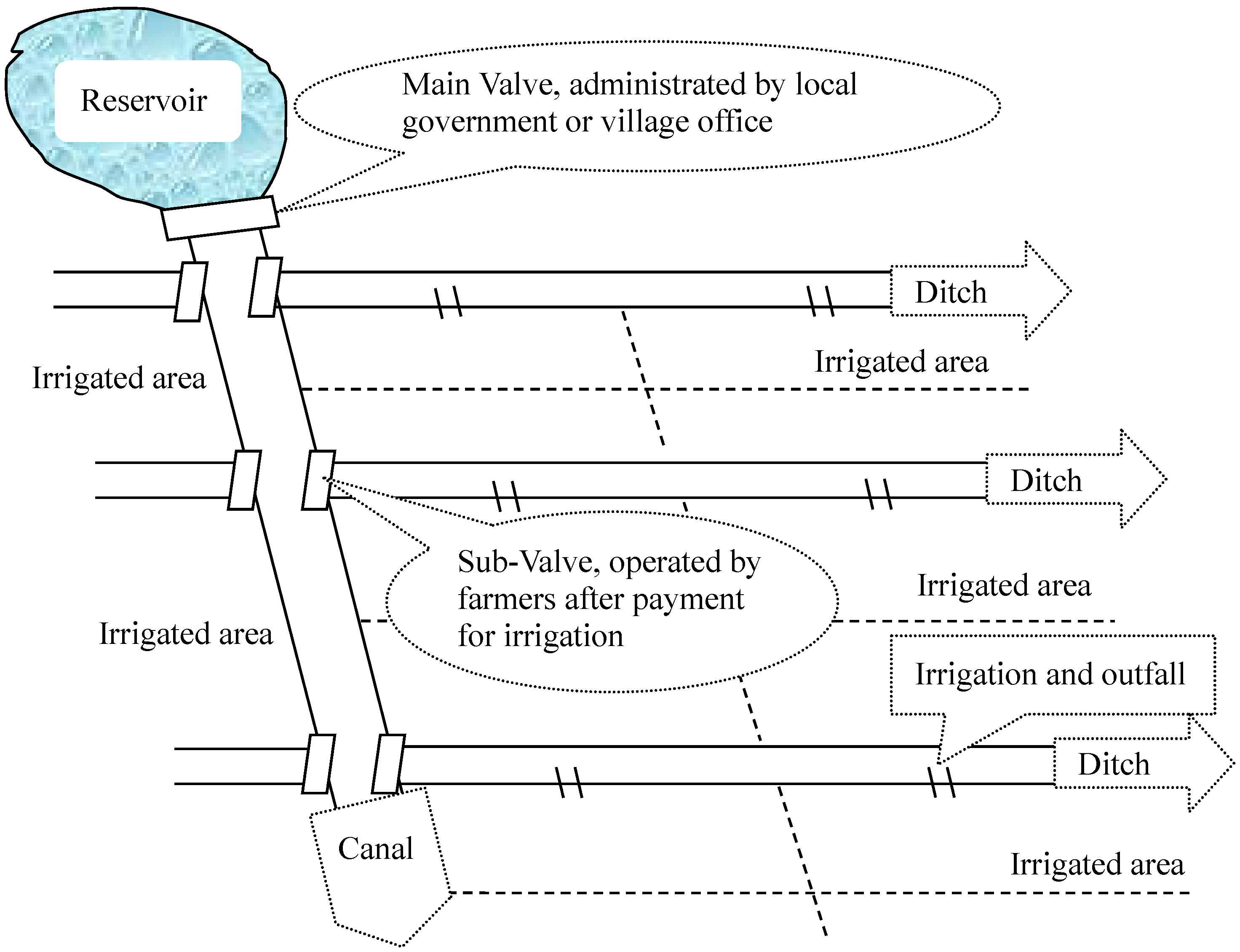
The reform of China’s water management is still in progress, and the pricing system is inadequate to the representation of the commodity attributes of water [
38]. The price distortion between agricultural water and non-agricultural water is usually neglected in previous water-CGE models of China. Moreover, little attention has been paid to China’s fragmented water management system, which is the main reason for the parallel pricing and separated supply for irrigation and pipe water. Previous CGE modeling studies involved China’s pricing system for water resources are rarely found in the literature.
3.2. Data and Modeling Framework
The water parallel pricing system is defined in both the dataset and model. This dataset essentially has the form of the 2007 Social Accounting Matrix (SAM) for China, which was contributed by Ge and Tokunaga (2011) [
39]. We introduced the 16 province’s equilibrium irrigation water inputs (from
Table 2) and their subsidies (from
Table 3) and also the production sector of pipe water into the SAM to construct the SAM with the irrigation waterfrom 16 provinces (SAM-16P, see
S1 in Supplementary Material File; for a simplified diagram, see
Table 4).
This model also refers to some agricultural CGE models to address the connection between agriculture and water, stated by Zhong, Okiyama and Tokunaga (2014) [
40], Akune, Okiyama and Tokunaga(2011) [
41], Okiyama and Tokunaga (2010) [
42] and Tokunaga
et al. (2003) [
43]. The detailed mathematical functions of this static CGE model with irrigation water from16 provinces (SCGE-16P) are presented in
Appendix.
The production module consists of 34 sectors, which were divided into two categories: (i) Agricultural sectors including farming and non-farming, allocated across agricultural labor, croplands and irrigation water from 16 provinces; (ii) Other sectors including industrial, construction and services, where pipe water are the inputs. It should be noted that non-farming agricultural sectors only employ agricultural labor but not croplands and irrigation water; and other non-agricultural sectors only employ non-agricultural labor and capital. The nested constant elasticity of substitution (CES) production structure is applied to all production sectors. Most of parameters in the SCGE-16P as in the standard CGE model were derived from calibration, with the exception of substitution elasticity (
) [
44].
Table 4.
Simplified social accounting matrix (SAM)-16P. Note: AGR = Agricultural sectors as activities/commodities, including paddy, wheat, corn, vegetable, fruit, oil seed, sugarcane, potato, sorghum and other crops and also animal husbandry, forestry, fishery and agriculture services; OTH = Other sectors as activities/commodities; WAP = Pipe water production sector as one of activities/commodities; 16WAR = 16 Provinces’ irrigation water as factor inputs; 16LAND = 16 Provinces’ croplands as factor inputs; 16AGRLB = 16 Provinces’ agricultural labor as factor inputs; NAGRLB = Non-agricultural labor as a factor input; CAP = Capital as a factor input; 16HHDRUAL = 16 provinces’ rural households; HHDURBN = Urban households; GOV = Government; ENT = Enterprise; S-I = Savings and Investment; DTAX = Direct tax; INDTAX = Indirect tax; 16SUBWAR = 16 Provinces’ subsidy for irrigation water; TAR = Tariff; ROW = Rest of the world.
| Unit: 0.1 billion yuan | Activities and Commodities | Factors | Institutions | Others | Total |
| AGR | OTH | WAP | 16WAR | 16LAND | 16AGRLB | NAGRLB | CAP | 16HHDRUAL | HHDURBN | GOV | ENT | S-I | DTAX | INDTAX | 16SUBWAR | TAR | ROW |
| Activities and Commodities | AGR | 6877 | 27,514 | 0 | | | | | | 6013 | 6301 | 342 | | 3581 | | | | | 666 | 51,294 |
| OTH | 13,348 | 503,647 | 590 | | | | | | 19,106 | 65,968 | 34,849 | | 109,503 | | | | | 94,875 | 841,886 |
| WAP | 9 | 837 | 41 | | | | | | 52 | 270 | | | −30 | | | | | | 1179 |
| Factors | 16WAR | 1823 | | | | | | | | | | | | | | | | | | 1823 |
| 16LAND | 157 | | | | | | | | | | | | | | | | | | 157 |
| 16AGRLB | 26,564 | | | | | | | | | | | | | | | | | | 26,564 |
| NAGRLB | 618 | 82621 | 244 | | | | | | | | | | | | | | | | 83,484 |
| CAP | 1115 | 115,819 | 229 | | | | | | | | | | | | | | | | 117,163 |
| Institutions | 16HHDRUAL | | | | | 157 | 26,564 | 5036 | 6651 | | | 793 | 8105 | | | | | | 905 | 48,211 |
| HHDURBN | | | | | | | 78,448 | 2328 | | | 5602 | 20,512 | | | | | | 2008 | 108,898 |
| GOV | | | | 1823 | | | | | | | | | 5700 | 11,965 | 38,519 | −1665 | 1433 | -12 | 57,761 |
| ENT | | | | | | | | 106,560 | | | | | | | | | | | 106,560 |
| Others | S-I | | | | | | | | | 22,013 | 34,199 | 16,053 | 69,163 | | | | | | −22,675 | 118,754 |
| DTAX | | | | | | | | | 1027 | 2158 | | 8779 | | | | | | | 11,965 |
| INDTAX | 48 | 38,396 | 75 | | | | | | | | | | | | | | | | 38,519 |
| 16SUBWAR | −1665 | | | | | | | | | | | | | | | | | | −1665 |
| TAR | 73 | 1360 | 0 | | | | | | | | | | | | | | | | 1433 |
| ROW | 2328 | 71693 | 0 | | | | | 1623 | | | 122 | | | | | | | | 75,766 |
| Total | 51,294 | 841,886 | 1179 | 1823 | 157 | 26,564 | 83,484 | 117,163 | 48,211 | 108,898 | 57,761 | 106,560 | 118,754 | 11,965 | 38,519 | -1665 | 1433 | 75,766 | |
Previous CGE models have provided a useful reference work for this study. Based on the CGE model with the croplands of 16 provinces [
39,
45], we incorporated irrigation water and pipe water by modeling the water parallel pricing system by means of integrated formulation where irrigation water acts as one of the factor inputs in the farming sectors and pipe water is consumed by all production sectors as an intermediate input and by households through their demand functions. Compared to previous CGE models, this model incorporates irrigation subsidy to indicate the price distortion between irrigation water and pipe water; irrigation water input and its subsidy are disaggregated into 16 groups for each of the 16 provinces. This gives the pipe water consumption of rural households. Thus, the water parallel pricing system is introduced into this model, in which irrigation water price is given at the level for which farmers are willing to pay and the subsidy is included. The supply of irrigation water is regulated by local government. Pipe water price is equal to the marginal cost of production, and pipe water supply is operated by its production sector. Therefore, the water parallel pricing system is represented by the parallel pricing processes of irrigation water and pipe water.
In China’s CGE modeling studies, the Cobb-Douglas function has been widely applied to represent the substitution between labor and capital in agricultural production (e.g., [
31,
32]); while in other production, the CES function is employed and its elasticity of this substitution has been estimated (e.g., [
46,
47,
48]). For the substitution between labor and capital (
), agricultural sectors have the Cobb-Douglas function, while non-agricultural sectors have the CES function with the elasticity given by Zhao and Wang (2008) [
46]. The substitution between non-agricultural labor and agricultural labor (
), as well as that among regional agricultural labor (
), are referred to Ge, Lei and Tokunaga (2014) [
45]. Furthermore, farming sectors employ the combinations of cropland and irrigation water (the land-water bundles) from 16 provinces following the Cobb-Douglas assumption [
45], and the irrigation subsidy is included in irrigation water price (see
Figure 4). We set
to denote that water pricing not a valid means of significantly reducing agricultural water consumption under water parallel pricing system [
49,
50]. Pipe water is combined with value-added input within the production function of non-farming agricultural sectors and other sectors, which faithfully reflects the characteristics of water-use efficiency in China. Water-use efficiency is highly relevant to value-added input, especially in industry, and therefore “water-use per unit of industrial value added” is used to represent water-use efficiency [
6] (see
Figure 5). We set
to represent a more direct influence of water pricing policy on the industrial production [
13]. The pipe water input in the farming sectors along with the irrigation water of “Other provinces” becomes the composite water demand of “Other provinces”. The reason for this setting is that those rural areas using pipe water for irrigation are very close to urban areas and thus were classified within “Other provinces”. We set
to assume that there is no difference between pipe water and irrigation water for farming production.
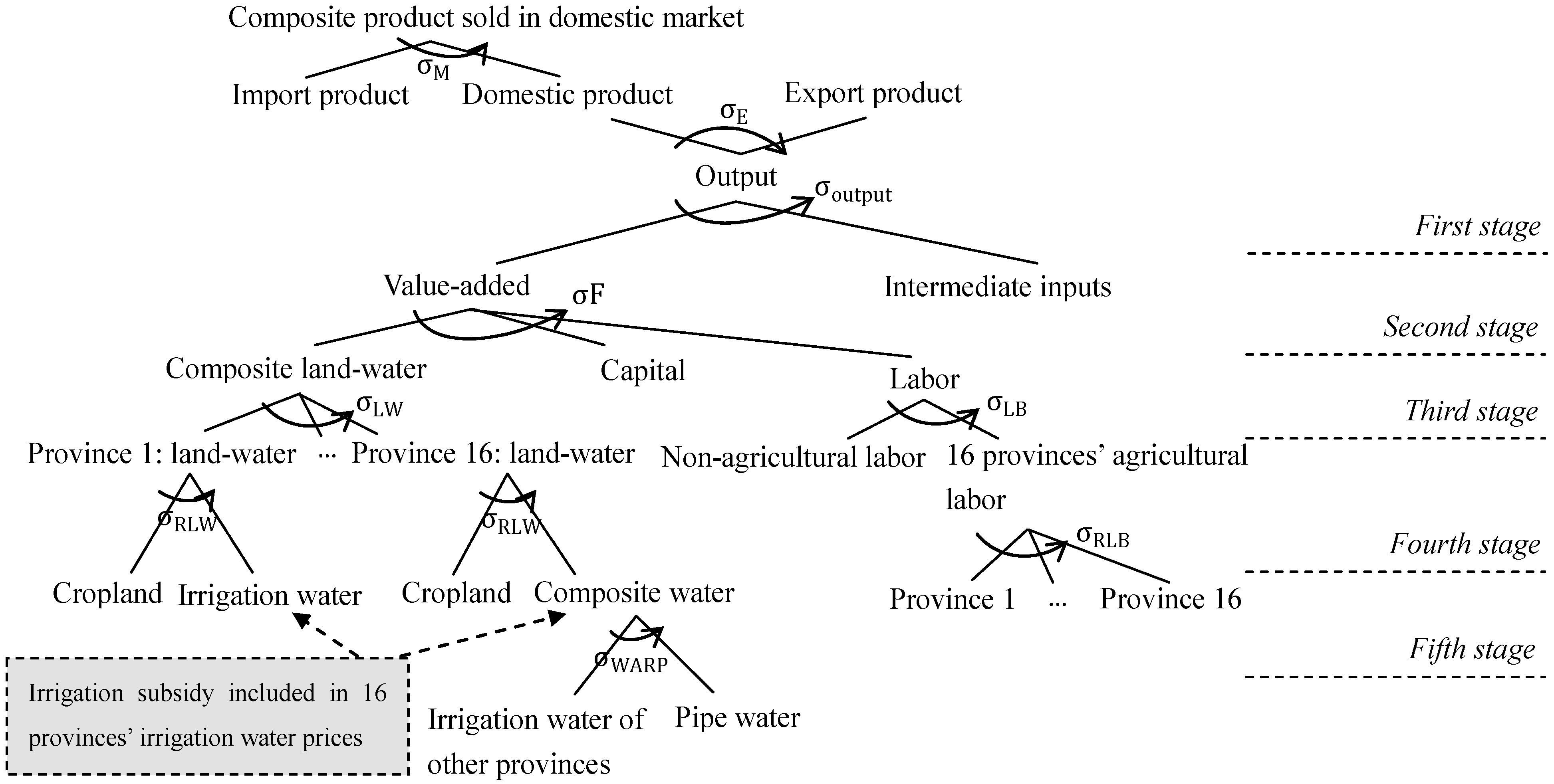
Figure 4.
Nested constant elasticity of substitution (CES) production structure of farming sectors. Notes: Province 1 = Guangdong; Province 2 = Jiangxi; Province 3 = Hainan; Province 4 = Yunnan; Province 5 = Guangxi; Province 6 = Henan; Province 7 = Jilin; Province 8 = Anhui; Province 9 = Heilongjiang; Province 10 = Hebei; Province 11 = Hubei; Province 12 = Chongqing; Province 13 = Sichuan; Province 14 = Inner Mongolia; Province 15 = Shandong; Province 16 = Other Provinces.
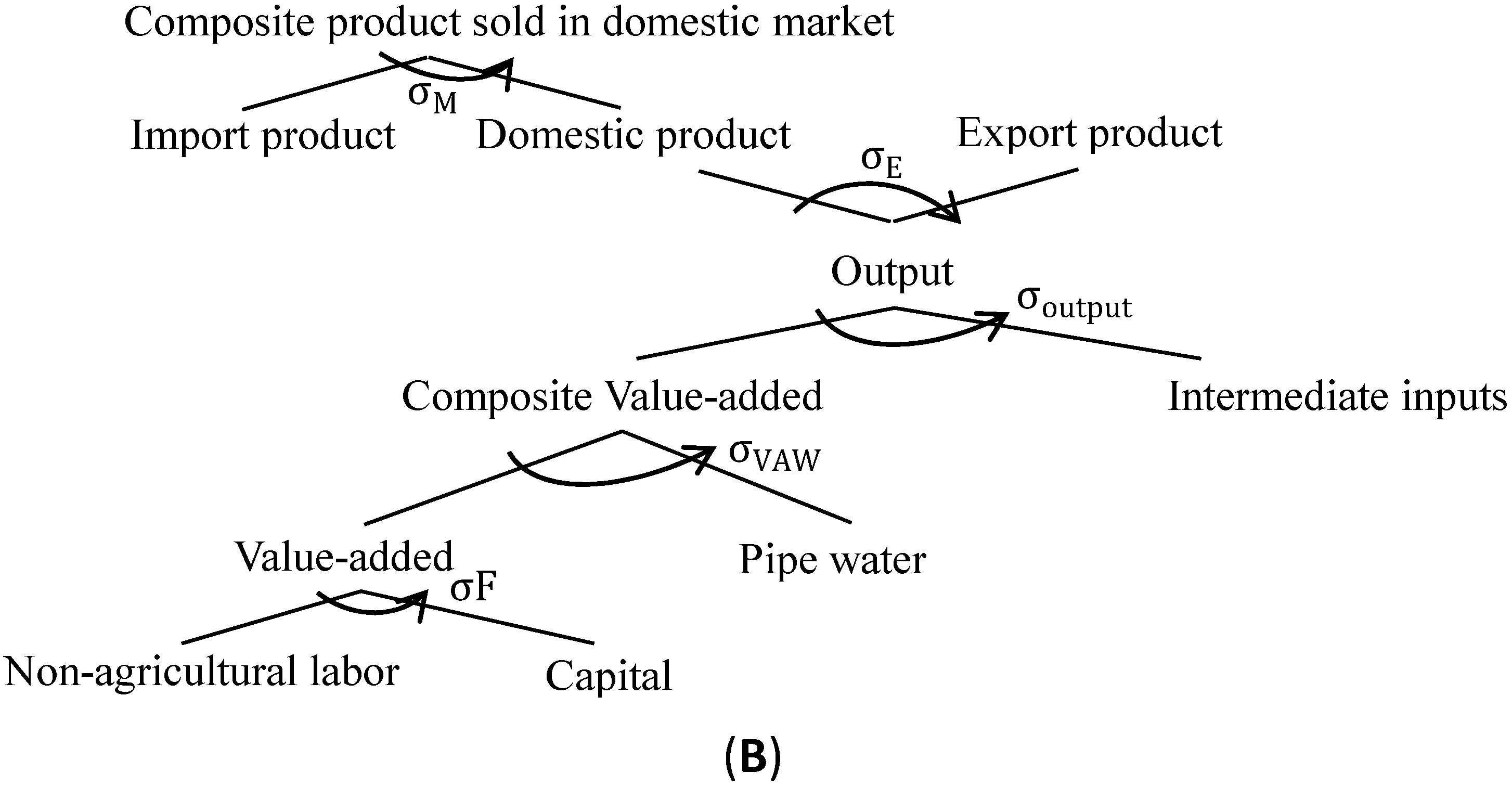
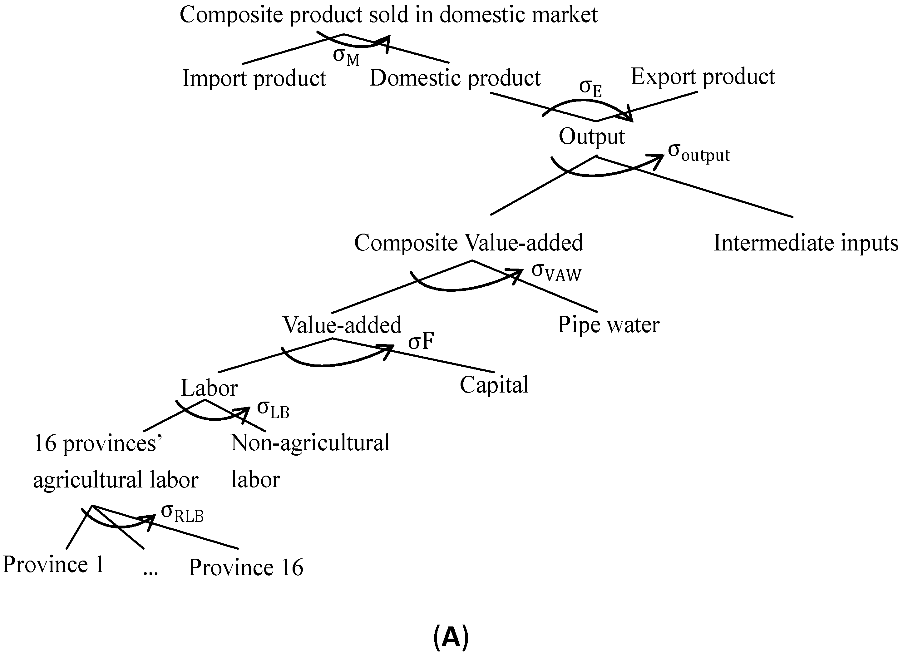
Figure 5.
Nested CES production structure of non-farming sectors. Note: Non-farming sectors including non-farming agricultural sectors (A) and Other sectors (B).
Figure 5.
Nested CES production structure of non-farming sectors. Note: Non-farming sectors including non-farming agricultural sectors (A) and Other sectors (B).
The total supply of irrigation water is exogenous to presenting the resource endowment owned by the government, and so the government receives total payments of the irrigation water supply from 16 provinces as a source of income. Total subsidies of irrigation water are also entered into the income function of the government with a negative value. However, pipe water supply is equal to the sum of the sectoral demand defined by a market clearing function.
Households are grouped by urban and the 16 province’s rural households (corresponding to the water, agricultural labor and land provinces). Their income comes from the payments of agricultural and non-agricultural labor, capital return, cropland’s return and the transfers from government and enterprises and also foreign countries. Their consumption behavior follows the Cobb-Douglas assumption. The Hicksian equivalent variation (EV) measures the changes in household welfare: if EV is positive, the simulation increases welfare; and if it is negative, the simulation decreases welfare.
SCGE-16P as an open-economy model follows a small-country assumption regarding that the world prices of imports and exports are exogenous. The domestic prices of imports and exports are in Chinese Yuan (RMB). Similar to most CGE models, domestic production of each commodity is divided into domestic and export products through a constant elasticity of transformation (CET) function (
, obtained from Zhai and Hertel (2005) [
47], is presented in
Figure 4 and
Figure 5). The domestic consumption of each commodity is composed of domestic and import products based on the Armington assumption (1969) [
51] (
, obtained from Willenbockel (2006) [
48], is presented in
Figure 4 and
Figure 5).Moreover, domestic consumption is separated by households, government and investment following the Cobb-Douglas assumption, respectively. Total investment is the sum of the savings obtained from households, enterprises and government, respectively. In particular, the model structure of farming products within the SCGE-16P is presented in
Figure 6.
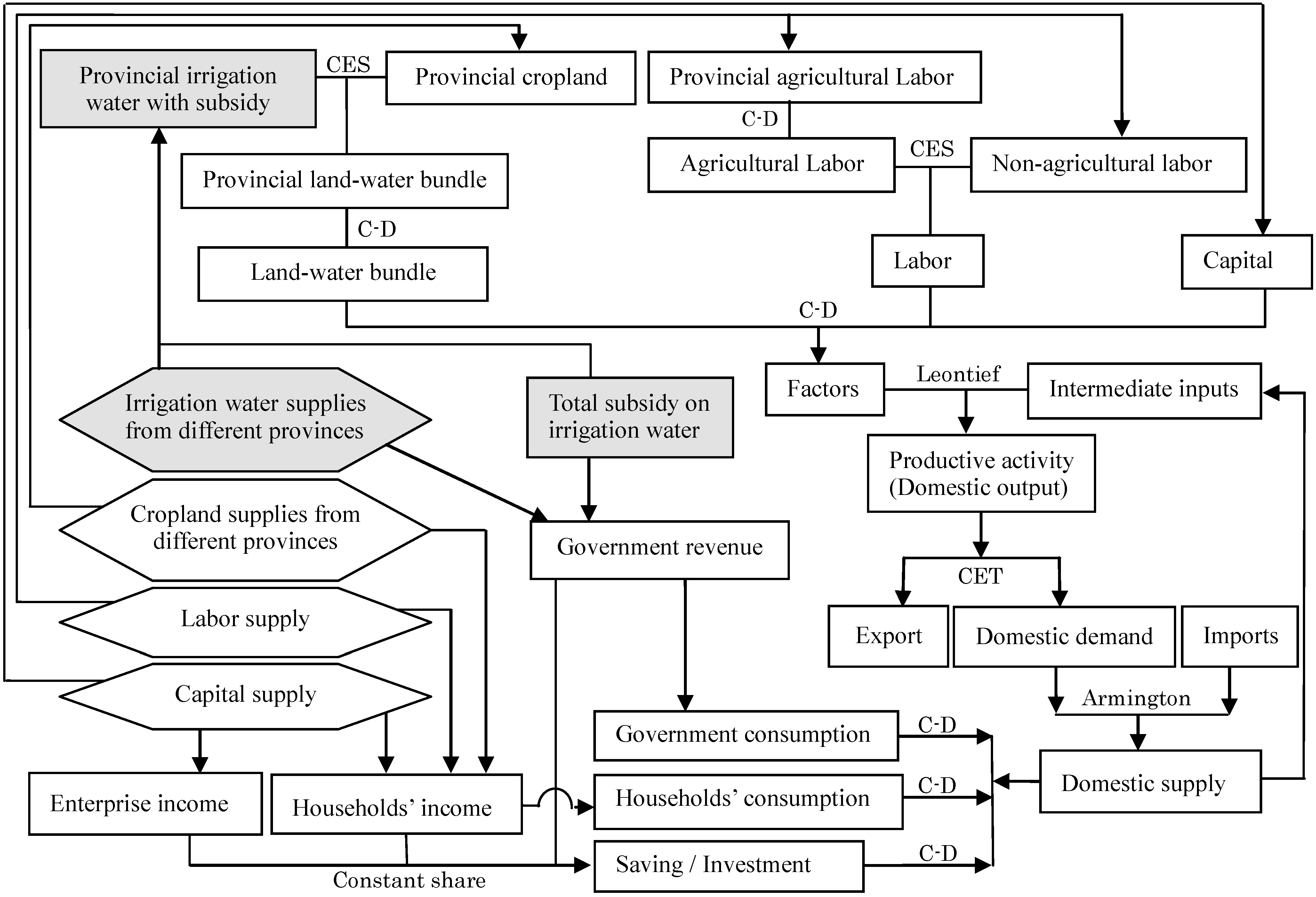
Figure 6.
Model structure for farming products in the SCGE-16P. Notes: C–D = Cobb–Douglas function; Leontief = Leontief function; CES (Armington) = the constant elasticity of substitution function; CET = the constant elasticity of transformation function; exogenous variables are circled by
![Water 07 03431 i001]()
; endogenous variables are circled by
![Water 07 03431 i002]()
.
Other assumptions are same as those for the standard CGE model [
44]. Moreover, all prices of commodities and factors in the base year are assumed to equal one. We excluded the non-agricultural labor market to follow Walras’ law, and the wage of non-agricultural labor is exogenously fixed as the numeraire price index. Sensitivity analysis, where abnormalities were not observed from the results, can be obtained from the authors upon request for the sake of brevity. This model was conducted within the GAMS (Generalized Algebraic Modeling System) software, and the GAMS codes can be found in another one of
Supplementary Material File, S2.


 ; endogenous variables are circled by
  .
.