Article

A Structurally Simplified Hybrid Model of Genetic Algorithm and Support Vector Machine for Prediction of Chlorophyll a in Reservoirs

1
State Key Laboratory of Water Environment Simulation, School of Environment, Beijing Normal University, Beijing 100875, China
2
Key Laboratory for Water and Sediment Sciences of Ministry of Education, School of Environment, Beijing Normal University, Beijing 100875, China
3
Chinese Academy for Environmental Planning, Ministry of Environmental Protection, Beijing 100012, China
4
Management Office of Miyun Reservoir, Beijing 101512, China
*
Author to whom correspondence should be addressed.
Water 2015, 7(4), 1610-1627; https://doi.org/10.3390/w7041610
Submission received: 13 January 2015 / Revised: 21 March 2015 / Accepted: 3 April 2015 / Published: 16 April 2015
(This article belongs to the Special Issue Hydro-Ecological Modeling)

Abstract

:
With decreasing water availability as a result of climate change and human activities, analysis of the influential factors and variation trends of chlorophyll a has become important to prevent reservoir eutrophication and ensure water supply safety. In this paper, a structurally simplified hybrid model of the genetic algorithm (GA) and the support vector machine (SVM) was developed for the prediction of monthly concentration of chlorophyll a in the Miyun Reservoir of northern China over the period from 2000 to 2010. Based on the influence factor analysis, the four most relevant influence factors of chlorophyll a (i.e., total phosphorus, total nitrogen, permanganate index, and reservoir storage) were extracted using the method of feature selection with the GA, which simplified the model structure, making it more practical and efficient for environmental management. The results showed that the developed simplified GA-SVM model could solve nonlinear problems of complex system, and was suitable for the simulation and prediction of chlorophyll a with better performance in accuracy and efficiency in the Miyun Reservoir.

1. Introduction

Water conflicts are key issues for sustainable water resources management. Under the dual effects of climate change and human activities, many water bodies are polluted to varying degrees, further exacerbating water conflicts [1,2]. Ecosystem studies such as water enhancement, water quality risk assessment, and early warnings have drawn much attention across the world [3]. As important engineering measures are developed to guarantee water supply, irrigation, electricity, and other functions, reservoirs can help solve these issues through the redistribution of runoff in both time and space; therefore, they are widely used throughout the world. Although water demands of each production department (e.g., industrial department, agricultural department, and so on) correspond to different water quality requirements, water quality always needs to be up to its appropriate standard in different water usage [4]. Accordingly, it is important to forecast water quality accurately, which could provide a scientific decision basis for reservoir management.
Chlorophyll a is an important component of algae organisms, and its concentration in water bodies is closely related to the type and the quantity of algae [5]. Therefore, as an important symbol of phytoplankton stock, concentration of chlorophyll a can reflect water nutritional status, making chlorophyll a one of the indicators in controlling the eutrophication of lakes and reservoirs. The minimum threshold concentration of chlorophyll a for eutrophic lakes identified by the Organization for Economic Cooperation and Development (OECD) is 0.008 mg/L. Consequently, there is a need to control the concentration of chlorophyll a in water to prevent potential eutrophication. For this reason, accurate prediction of chlorophyll a is a worldwide concern.
The generation mechanism of chlorophyll a in water is accordingly complex, which is closely related to ecological, environmental, and societal activities. Therefore, the elements involved in the prediction for chlorophyll a in water are complex accordingly. In the existing literature, prediction models for chlorophyll a mainly included two categories: statistical regression models [6] and mechanism models [7]. Statistical regression models were established with the applications of statistical correlation analysis theory and methods. This means that the sample size had a major influence on prediction accuracy. Moreover, these models usually applied a linear relationship to simplify complex problems, leading to unsatisfactory prediction results under the situation when the limiting factors of chlorophyll a changed. Mechanism models mainly included the nutrient model, phytoplankton model, and ecological dynamic models such as CE-QUAL-ICM, WASP, CAEDYM, AQUATOX, and ECOPATH [8,9,10]. Based on the principle of hydrodynamics and ecosystem dynamics, these models comprehensively considered the interaction mechanisms among indicators of water resources system and ecosystem, and then predicted the future development of the system accurately. However, these models also had a high demand for data quantity, which was inconvenient for model calibration and verification, leading to a decline in reliability and applicability. Furthermore, due to uncertainty factors such as the concentration of phosphorus input from non-point source pollution, the prediction of chlorophyll a based on deterministic differential equations was not reasonable [11]. For this reason, the uncertainty of input parameters and the nonlinearity of the system required further consideration when constructing models.
To improve the accuracy and efficiency of nonlinear system simulations, intelligent algorithms have been applied in recent years [12]. Widely used intelligent algorithms include the artificial neural network (ANN), the genetic algorithm (GA), the particle swarm algorithm, the wavelet theory, and the projection pursuit algorithm, etc.; these intelligent algorithms overcome the uncertainty to a certain extent with high simulation precision. In recent years, the support vector machine (SVM) algorithm, which is a new type of machine learning tool based on statistical learning theory, has drawn more attention [13]. This intelligent algorithm can solve nonlinear system problems and has reasonable generalization ability when using small samples, ameliorating the weaknesses of the above intelligent algorithms, e.g., large sample size requirements and being susceptible to underfitting and overfitting the data for the ANN. The SVM has demonstrated promise for applied studies of water environments, especially for the prediction of hydrologic factors, such as wave height [14], inflow [15], and water levels [16]. Previous studies of chlorophyll a based on the SVM algorithm often focused on the retrieval of chlorophyll a in water [17], although very few results of chlorophyll a prediction have been reported [18]. Furthermore, chlorophyll a is affected by many factors, and irrelevant and redundant information is often hidden in the time series of high dimensional feature vectors, leading to structurally complex models and a decrease of analysis precision and application efficiency of the SVM model when using conventional modeling processes [19]. To simplify the model structure and avoid the interference of redundant information in chlorophyll a forecasts, it is desirable to obtain more accurate and reliable prediction results by using SVM models with the most relevant influence factors as input vectors and simple structures. Feature selection is an important approach for getting structurally simplified model by removing those redundant parameters. Cho et al. [20] used principal component analysis (PCA) to extract variables for the prediction model of chlorophyll a. Compared to conventional parameter extraction approaches such as PCA, the GA has a distinct advantage in fast random search. Thus, the SVM model can be expected to get satisfactory prediction results through combing the GA to extract feature variables and simplify the model structure in such complex water bodies as reservoirs, whose water quality variations likely result from a combination of multiple factors. However, the GA-SVM hybrid model needs to be further developed for nonlinear water resources system.
This study developed a hybrid model of GA and SVM algorithms to predict chlorophyll a in the Miyun Reservoir of northern China. Based on the feature selection with the GA, we extracted appropriate input vectors, so that the redundant information was effectively eliminated with the simplified model structure. This model could analyze water quality and its change trend with reliable results, and was of great practical significance in preventing water pollution accidents.

2. Study Area and Data Description

The Miyun Reservoir is located in the Miyun County of Beijing City. Built in 1960, it is the largest reservoir and is a unique surface source of drinking water in Beijing City (Figure 1). In addition to functioning as a water supply, the Miyun Reservoir also provides irrigation, flood control, power generation, aquaculture, tourism, and other comprehensive benefits. The Miyun Reservoir’s surface area is 183.6 km2, its maximum depth is 153.93 m, and the maximum volume of reservoir storage is 3.349 × 10¹⁰ m3. Monitoring data shows that in recent years, the total phosphorus concentration in the reservoir fluctuated between 0.010 and 0.025 mg/L, which means the nutrition status of the water is at a mesotrophication to oligotrophication level. The total nitrogen concentration ranges between 0.62 and 1.43 mg/L, indicating that the nutrition status is at a mild or moderate eutrophication level. Planktonic algae have rich diversities, and the dominant population in various periods is different in the Miyun Reservoir. As for cyanobacterium, from 2001 to 2003 it was the dominant algae from September to October [21]; from 2008 to 2010, it was the dominant algae from June to September [22,23]. Considering the current water quality situation, we should take effective measures to alleviate adverse influences resulting from climate change and human activities on the reservoir.
Figure 1. The Miyun Reservoir in northern China.
Water 07 01610 g001
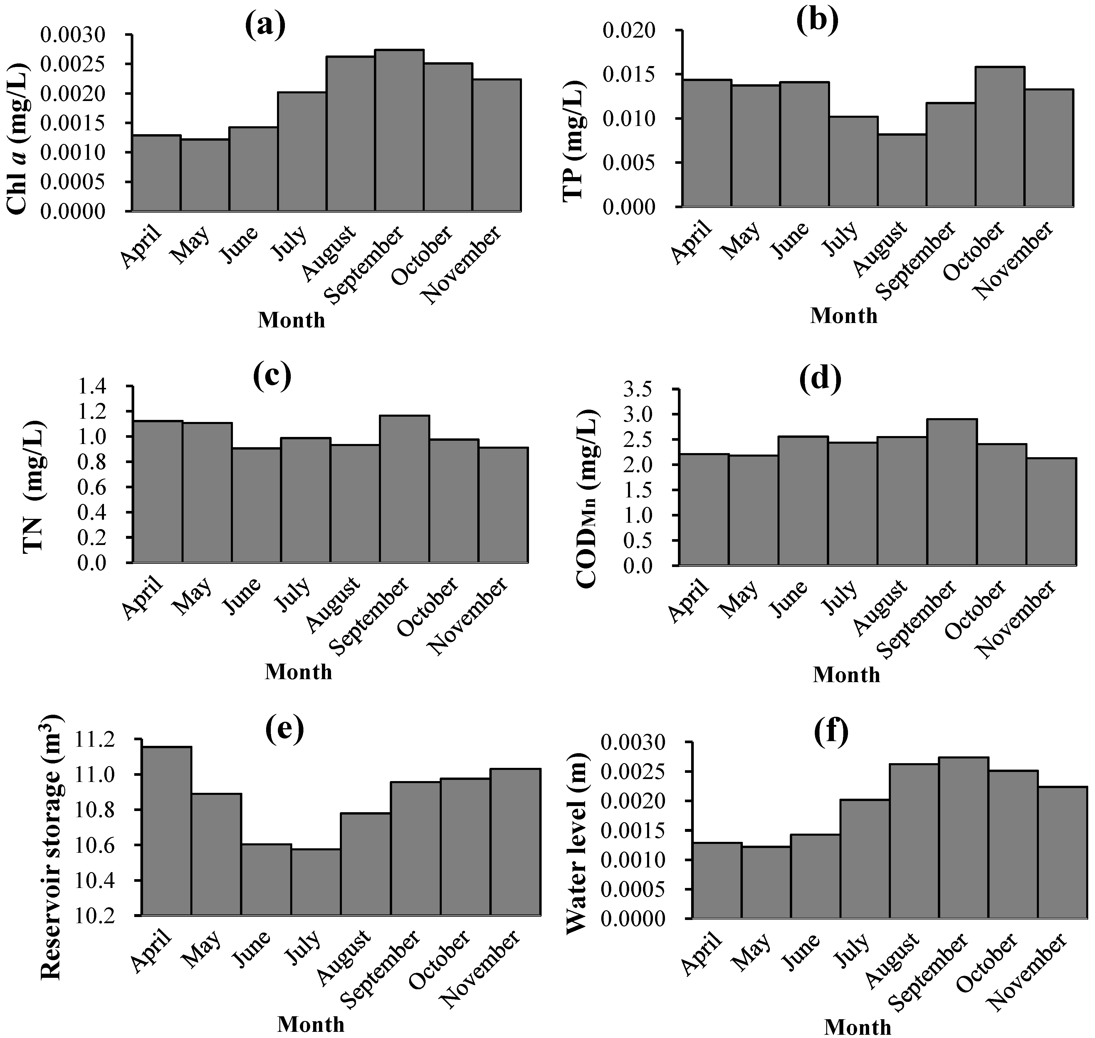
In this paper, the Baihe Key Dam in the Miyun Reservoir is taken as the research area. Data for the model establishment and calibration are from the monitored data, including water quality indicators (i.e., chlorophyll a in water, total nitrogen, total phosphorus, permanganate index, and dissolved oxygen), hydrological indicators (i.e., water temperature, pH, transparency, flow, reservoir storage, inflow, outflow, and water level), and meteorological indicators (i.e., precipitation and temperature). The monthly data from 2000 to 2010 were obtained from the Miyun Reservoir Management Office. Because the Miyun Reservoir is frozen for the period from December to March, the prediction of chlorophyll a focused on the period from April to November in each year, and other indicators in the SVM model corresponded to these months. The average monthly variations of parts of these indicators are shown in Figure 2.
Figure 2. Water environmental situation in Miyun Reservoir: (a) Concentration of chlorophyll a; (b) TP concentration; (c) TN concentration; (d) CODMn concentration; (e) reservoir storage; and (f) water level.
Water 07 01610 g002

3. Methods

Originally proposed in 1985 by Cortes and Vapnik, the SVM algorithm was widely used to solve highly nonlinear classification and regression problems with good generalizability [24]. The SVM algorithm can be easily applied to other machine learning problems such as function fitting. It is based on the VC dimension theory and the structure risk minimum principle of the statistical learning theory. By seeking the best compromise among the complexities in the model with a limited sample (i.e., learning accuracy of particular training samples) and learning ability (i.e., learning ability to identify random sample), the SVM algorithm can achieve the best generalization ability. There are many meteorological and hydrological parameters that influence chlorophyll a. To avoid blindness in selecting the input vector during the process of chlorophyll a prediction, this study firstly took feature selection to determine the best input vectors of prediction model with the GA, and then constructed the SVM model with a simplified model structure to achieve the purpose of improving prediction accuracy.

3.1. The Flow Chart for Developing a Simplified Structural GA-SVM Hybrid Model

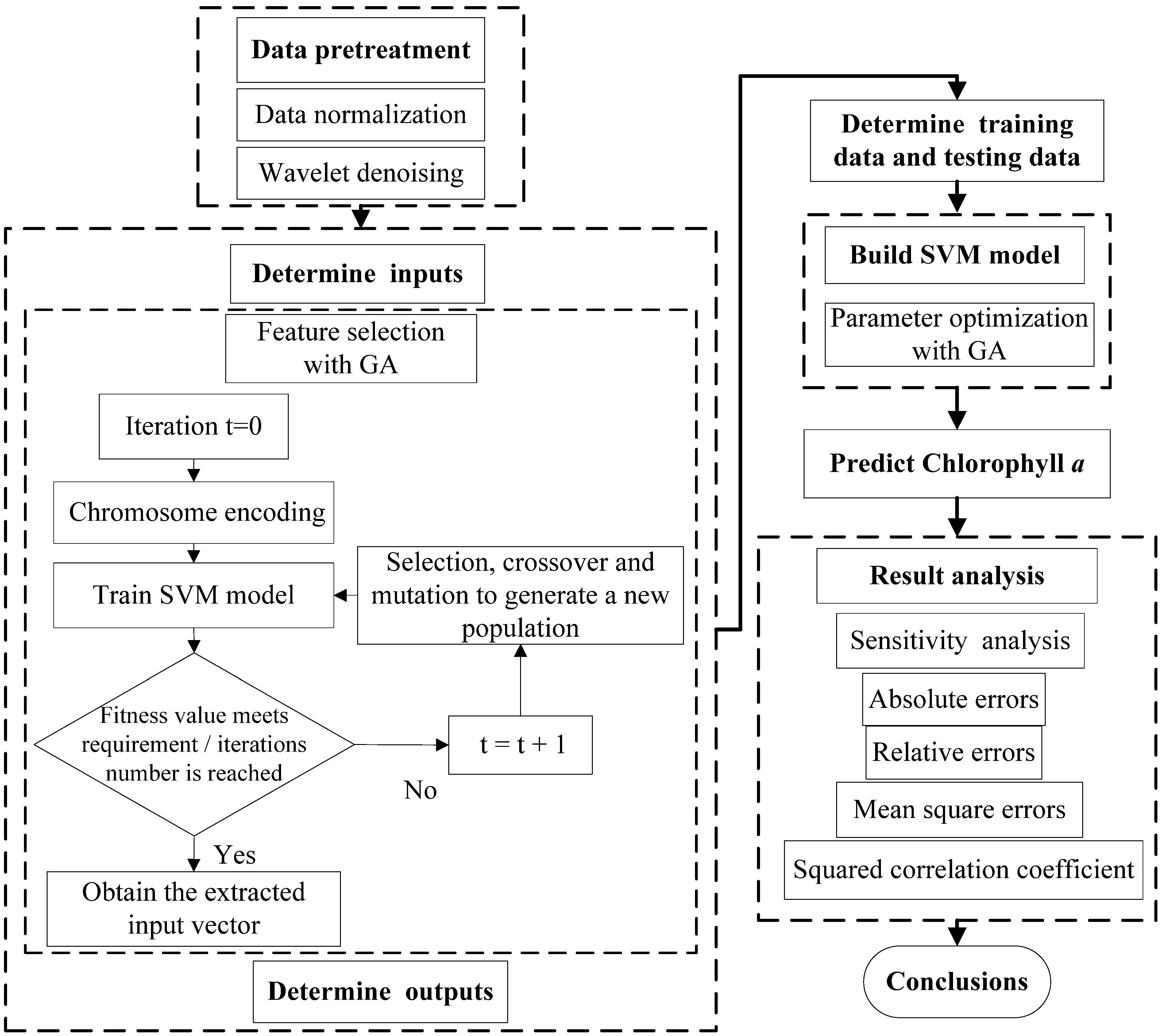
The penalty factor and kernel function parameters of the SVM model may directly influence simulation results. This study developed a SVM model by using the GA to optimize the input parameters in the SVM model and extract feature parameters with the aim of simplifying the model structure. The flow chart of the simplified structural SVM model based on the GA is shown in Figure 3. After data pre-treatment, the input and output vectors were determined, and the sample set was divided into a training data set and a testing data set. The GA was applied to optimizing the parameters of the SVM model and extracting input vectors. The SVM model was trained and calibrated with optimal parameters, then used to predict chlorophyll a in the water. This study applies the LIBSVM software package developed by Lin Chih-Jen et al., of Taiwan University to run the program on the MATLAB platform [25].
Figure 3. The flow chart for developing simplified structural GA-SVM hybrid model for chlorophyll a prediction.
Water 07 01610 g003

3.2. Construction of Chlorophyll a Prediction Model Based on the SVM Algorithm

This paper applied the principle of the SVM algorithm to establish a prediction model for chlorophyll a in the Miyun Reservoir. The basic principle of the SVM algorithm was to first select a nonlinear mapping algorithm as a kernel function, through which the input vectors were mapped into a high dimensional feature space, and in this space simpler linear regressions can replace complex nonlinear regressions of the original input space [26]. Then an optimal decision function was produced in the feature space to realize the nonlinear decision function of the original input space, and finally the linear learning method can be applied to solve the classification and regression problems in the input space. This process can be expressed as:
y = f ( x , w ) =   w ( x ) + b ,
where y is the output, y R; x is the input vector, x Rn; w is the matrix of the regression weight vector; is a non-linear function by which x is mapped into a high dimensional feature space; b is a bias; and b and w can be obtained with Equation (3). In the mapping process, a kernel function k ( * , * ) can be constructed by k ( x , x ' ) =   ( ( x ) ( x ' ) ) . Therefore, we only need to replace the x or xi of the original space with ( x )   or ( x i ) , while it is not necessary to know the explicit expression of nonlinear mapping . In this study, we selected radial basis function (RBF) as the kernel function:
K ( x , x i ) = e x p ( γ x x i 2 ) ,
where xi is the input vector, x Rn; and γ is the parameter of the RBF kernel function.
In Equation (1), the concentration of chlorophyll a in reservoir water was selected as y in the SVM model, whereas other water quality factors, hydrological factors, and meteorological factors were selected as x in the SVM model. In this way, the concentration of chlorophyll a was predicted based on the other factors. To solve Equation (1), the following regularized risk function (i.e., Equation (3)) was used. These constraints ensured the regression errors of the samples being within the area that was delineated by the error tolerance and the slack variables. Equation (3) can be solved with the Lagrange technique.
Minimize
1 2 w 2 + C n = 1 N ( ξ n + ξ n * )
subject to
{ y i W T ( X i ) b ε + ξ i W T ( X i ) + b y i ε + ξ i * ξ i ,     ξ i * 0 } i = 1 , 2 , , N ,
where C is a penalty parameter that determines the penalty degree for the sample classification errors in the optimization problem; N is the number of the samples of { x n , y n } n = 1 N ; ξ n and ξ n * are slack variables that penalize training errors by the loss function over the error tolerance (ε); ξ n represents the upper training errors subject to ε ; ξ n * represents the lower training errors subject to ε; ξ n and ξ n * can be calculated with Equation (3); and was normally set to 0.001.
Overall, the chlorophyll a simulation with the SVM model depended on the ability to learn the nonlinear causality between the historical data of the concentration of chlorophyll a and its influencing factors (i.e., other water quality factors, hydrological factors, and meteorological factors). The modeling process for the SVM model was introduced below.
Step 1. Determine chlorophyll a as the output value of the prediction model, with the other indicators as input values:
ρ C h l a = F ( S , W I , W O , L , T P , T N , C O D M n , D O , T W , p H , S D , T A , P ) ,
where S is reservoir storage, WI is inflow, W0 is outflow, L is water level, TP is the concentration of total phosphorus in water, TN is total nitrogen in water, CODMn is permanganate index in water, DO is the dissolved oxygen concentration in water, TW is water temperature, pH is hydrogenion concentration of water, SD is water transparency, TA is temperature, and P is precipitation.
Step 2. Before establishing the SVM model, to extract useful information in the original data and determine the most reasonable and relevant input vectors of the prediction model, this study applied data normalization, wavelet denoising, and feature selection for the data pre-treatment in the MATLAB software. To test the prediction ability of the SVM model, the sample set was divided into separate training and testing sets. Data between 2000 and 2004 were used as the training set, and those between 2005 and 2010 as the testing set. Thus, the testing set data were independent and not used to train the model. In the parameter optimization, the initial conditions of the GA were set: the biggest evolution generation was 100, the largest population was 20, the gap of genetic algorithm was 0.9, and the k-fold cross-validation number was 5.
Step 3. To determine the effect of each input indicator to the prediction model, we carried out sensitivity analysis of the chlorophyll a prediction model. The analysis method was to change a particular input variable (increase or decrease by 10%) while the other input variables remained fixed and then applied the established SVM model to re-predict; the variable of the sensitivity model was obtained by calculating the relative changes in chlorophyll a with the output value.
Step 4. To eliminate the irrelevant and redundant information hidden in the time series of high dimensional feature vectors, and reveal the more representative features that influenced the concentration of chlorophyll a in the Miyun Reservoir, we applied feature selection to the input vectors of the SVM model for chlorophyll a simulation by using the GA. Subsequently, we established the hybrid SVM model using the extracted feature vectors and improved prediction accuracy, generalization ability, and efficiency.

3.3. Feature Selection and Parameter Optimization Based on Genetic Algorithm Optimization

The feature means each attribute of the data set. Too many features will increase the complexity of the work, while the accuracy of data mining may not be improved. To pick out the most representative and effective feature vectors of the chlorophyll a prediction model, we used the GA for feature selection. In addition, considering that the SVM model did not provide a method for selecting the parameter in the RBF kernel function and the penalty parameter (C), we used the GA for optimizing these two parameters in the SVM model. The principle of the GA is based on a specific operation for the structure of objectives, according to a predefined criteria function, to improve the new population by comparing it with the original one. In the process of generation, proper coding was used and the operator was applied to imitate the path of natural selection. Reproduction, crossover, and mutation were taken to operators in the current population [27]. Procedures of feature selection and parameter optimization with applications of the GA were as follows.
Step 1. Chromosome encoding. In the selection and optimization process, the iterations were set to zero. Chromosomes were encoded with binary coding. Each operator was composed of N codes, where N is the number of characteristic vectors or SVM parameters that need to be optimized. When a number in the operator was 1, it represented the characteristic vector and the parameter was selected; otherwise it was not selected, and the initial population was generated randomly.
Step 2. Evaluation of the fitness function value. Determine the square of the root mean square error in the training phase as the objective function for the fitness value. Then, calculate the fitness function value of the current generation. Choose a certain adaptation level, retaining the individuals whose fitness function value is greater than the adaptation level; these individuals compose the next generation.
Step 3. Selection, crossover and mutation of operators. Apply genetic operation of selection, crossover, and mutation to individuals in the group; the next generation was produced after the genetic optimization.
Step 4. Termination judgment. If the iteration number was greater than the set value, or the accuracy of the fitness function value reached the expected value, then terminate the iteration [28]. The extracted features and the optimal model parameters were then determined.

3.4. Model Calibration

In order to analyze the performance of the model, four indicators—The absolute error (AE), relative error (RE), root mean square error (RMSE), and square of correlation coefficient (R2)—Were selected to evaluate the fit and prediction effect of the model. AE represented the deviation between monitoring and prediction values, and RE was the ratio of AE and monitoring values, reflecting the objective accuracy of measurement results. RMSE reflected the performance of the prediction model, i.e., generally, the smaller the RMSE the better the performance. R2 represented the degree of linear relevance among the variables, i.e., the closer R2 was to 1 the higher the relevance. The expressions of these four indicators were as follows:
AE = | y i y ^ i |
RE = A E y i × 100 %
RMSE = 1 n i = 1 n ( y i y ^ i ) 2
R 2 = 1 i = 1 n ( y i y ^ i ) 2 i = 1 n ( y i y ¯ ) 2
where yi is the real value of the data set, y ^ i is prediction value, y ¯ is the average of the original data, and n is the amount of data for the testing set.

4. Results and Discussion

4.1. Wavelet Denoising

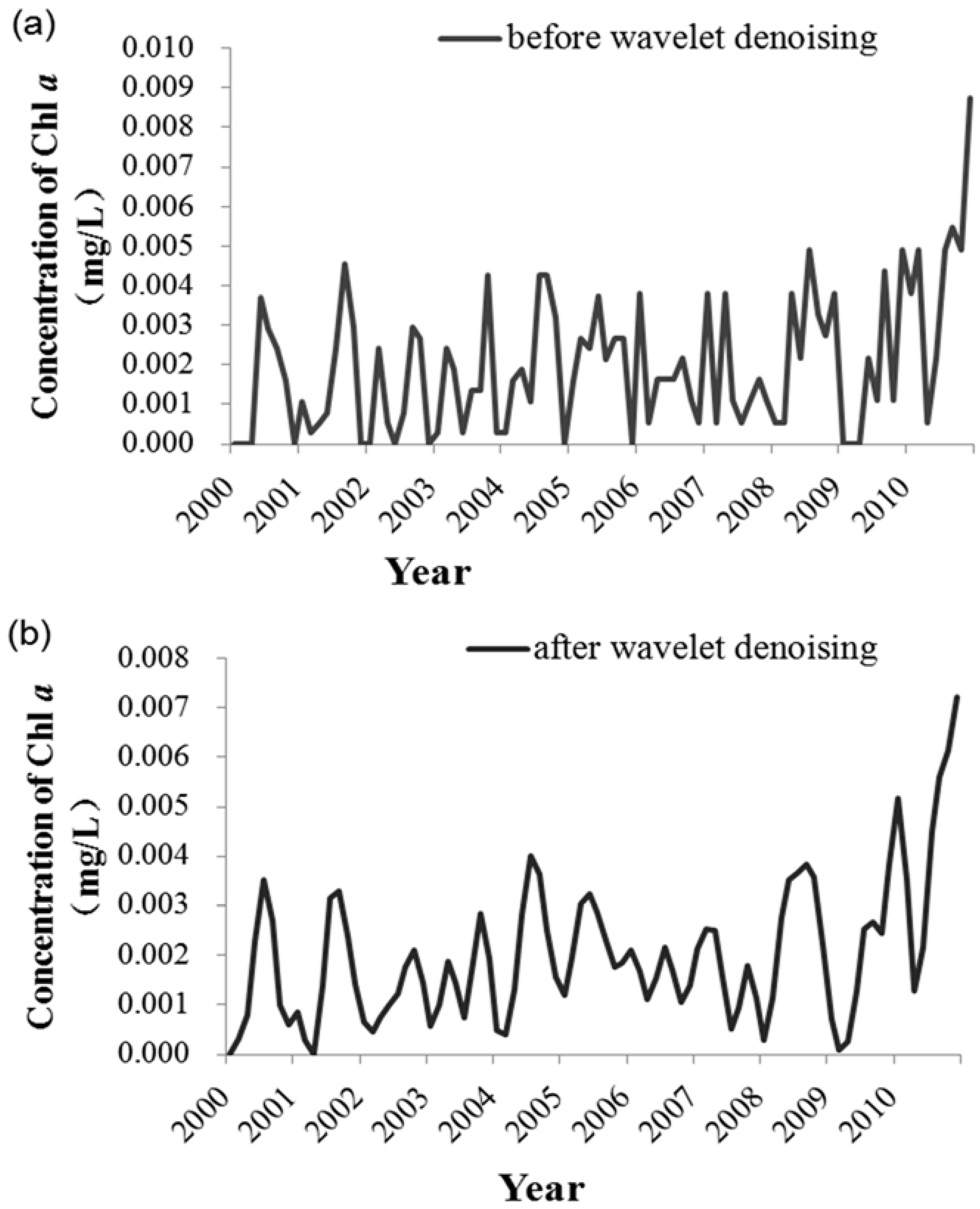
The results of applying the wavelet denoising method to the original data of chlorophyll a are shown in Figure 4. The upper and lower figures represented the time series data before and after the denoising, respectively. It was clear to see that after wavelet decomposition and reconstruction the low frequency characteristics of the original data were preserved, while eliminating the high frequency data. After this process, the abrupt change points of the time series data were smoothed, and the main information regarding the concentration of chlorophyll a was well preserved.
Figure 4. Comparisons of before and after the wavelet denoising.
Water 07 01610 g004
The noise of the original data about chlorophyll a was mainly caused by the errors in sampling and deviations in experiments due to unsuitable experimental conditions and improper operation caused by human errors. The wavelet denoising was realized through multi-scale decomposition of sequence data and reconstruction. The original signal was decomposed into a series of low frequency and high frequency components by using the wavelet decomposition, and the noise of chlorophyll a’s raw data was concentrated in the high frequency components. The high frequency components were processed with threshold, and the low frequency components were reconstructed to obtain the smooth data series. Because the low frequency components could preserve the details of the original data, excessive deviations can be avoided in data applications. Therefore, it was reasonable and concise to use the time series data of chlorophyll a after the wavelet denoising as input variables of the SVM model, without the loss of important information.

4.2. Results of Sensitivity Analysis and Feature Selection

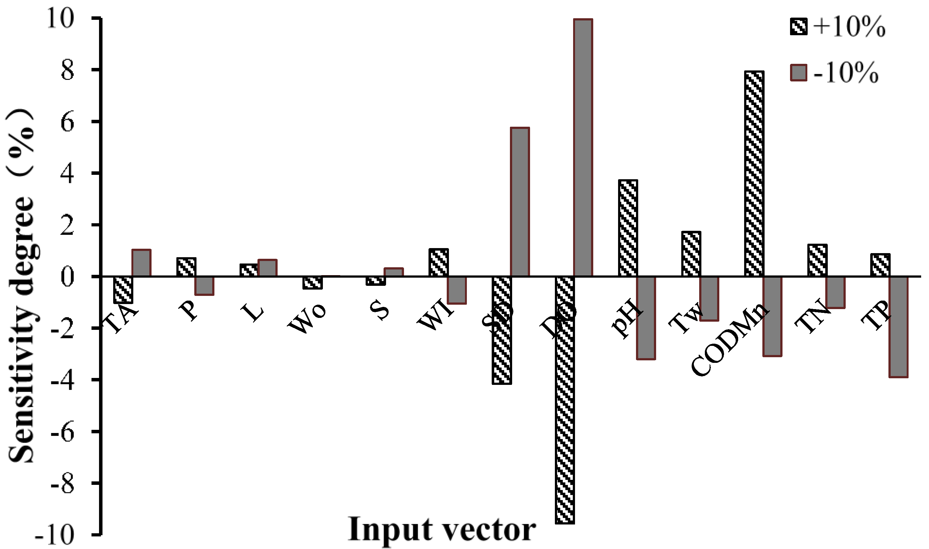
The use of the GA aimed to automate and enhance SVM designing process. The results of parameter optimization indicated that the optimal penalty factor C was 1.0737, and the optimal parameter γ in RBF kernel function was 1.0005. The final SVM model was established based on these results. Figure 5 shows sensitivity analysis results for input vectors of the SVM model. It can be seen that when the values of eight parameters (i.e., rainfall, water level, inflow, pH, water temperature, permanganate index, total nitrogen, and total phosphorus) increased by 10%, the sensitivity degree was greater than zero, which meant the prediction of chlorophyll a showed a positive correlation. Alternatively, when the values of the other five parameters (i.e., temperature, outflow, reservoir storage, dissolved oxygen, and transparency) increased by 10%, the sensitivity degree was less than zero, which meant the prediction of chlorophyll a showed a negative correlation. These correlations coincided with the mechanism of action for hydrology and water quality. Compared with other feature vectors, the prediction model for chlorophyll a in the Miyun Reservoir water had greater sensitivity to dissolved oxygen, transparency, permanganate index, pH, temperature, total nitrogen, and total phosphorus. It should be noted that the variations of transparency and dissolved oxygen were the results of the change in chlorophyll a.
Figure 5. Sensitivity analysis for input vectors of the SVM model.
Water 07 01610 g005
Four parameters, i.e., total phosphorus, total nitrogen, permanganate index, and reservoir storage, were extracted through feature selection. The results of the feature selection were consistent with those of the sensitivity analysis. Compared with other studies, although the influence factors of chlorophyll a were different for various research objects, two factors including the concentration of TN and TP were always main factors. For example, Canfield [29] applied statistical analysis to pick out the total phosphorus concentration and the total nitrogen concentration as the explanatory variables in their developed prediction model of chlorophyll a.
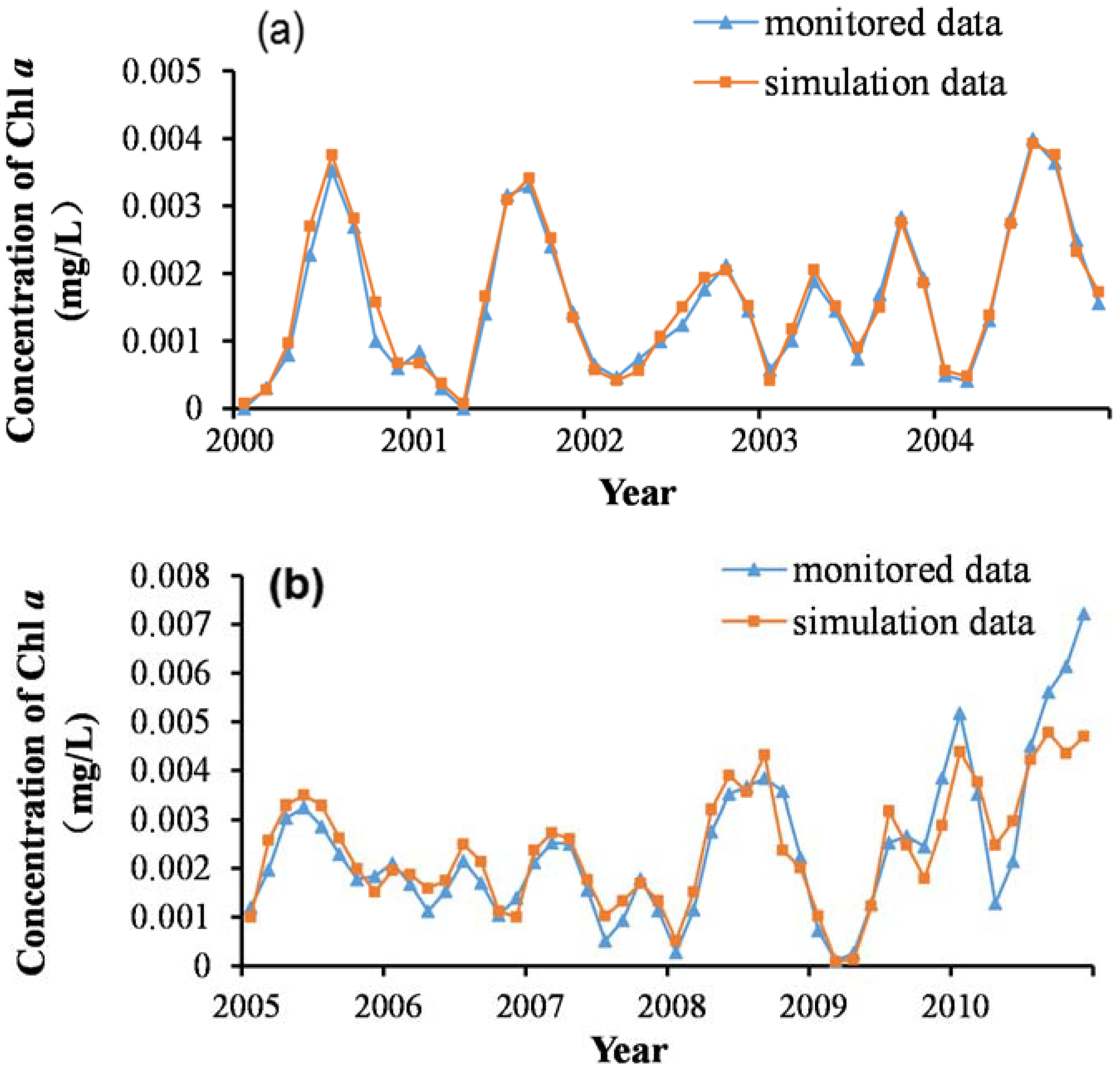
With these four parameters as the input vectors, the simplified SVM model was constructed. Figure 6a shows the results of the model training process. It can be seen that the simulation values are perfectly consistent with the monitored values, with the exception of a bias in the extreme points. Accordingly, the RMSE was only 0.00017, and the R2 was 97.33%. After the SVM prediction model was trained, chlorophyll a in the Miyun Reservoir was predicted for the period between 2005 and 2010. In Figure 6b, we can see that from 2005 to 2009, the simulation effect was passable. However, in 2010 the simulation effect was not satisfactory. Calculations showed that the RMSE of the testing set was 0.000641 and the R2 was 81.97%. From 2005 to 2009, the RMSE was 0.0004 and the R2 was 85.96%; however, in 2010, the RMSE was 0.0013 and the R2 was only 79.00%. This was primarily related to the fluctuations and periodicity of the monitored data. For the training data set, from 2000 to 2004, the concentration of chlorophyll a generally showed a peak in the middle of the year, but there was no obvious periodic trend for the concentration of chlorophyll a in the testing data set. In addition, in 2010 the concentration of chlorophyll a in the Miyun Reservoir was relatively higher compared with previous years. During April and for the period from August to November, the concentration of chlorophyll a was anomalously high, exceeding 0.004 mg/L, whereas in the training data set, the concentration of chlorophyll a had never achieved this level. Therefore, the SVM model was sensitive to the data. To explore which indicators were most relevant to chlorophyll a, sensitivity analysis for each input vector of the model was conducted.
Figure 6. Training and prediction results of the SVM model: (a) training results and (b) prediction results.
Water 07 01610 g006

4.3. Relative Errors of the SVM Model

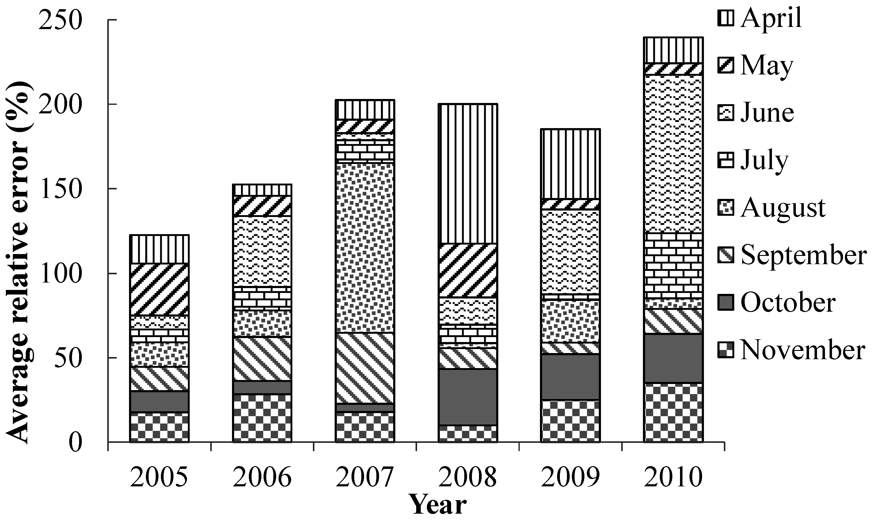
Figure 7 shows the relative errors in each testing year of the SVM prediction model. Overall, the relative error between 2005 and 2009 was smaller than that in 2010. This indicated that the model had improved prediction accuracy during the early part of the testing data. This result was related to the variations in the testing data. The first five years of the testing data were consistent with the training data with regard to the amplitude, cycle, and peak values. However, data in the last year did not exhibit regularity, as evidenced by the notable fluctuations in each month. Given the obvious fluctuation in the overall trend, the average relative error of the prediction in 2010 was the largest.
Figure 7. Average relative errors for each year.
Water 07 01610 g007
To analyze the errors of chlorophyll a prediction in different months, the monthly average relative error of the SVM model was compared between April and November (Figure 8). Prediction results showed that the average relative errors from April to November were 29.10%, 15.90%, 35.84%, 14.64%, 27.53%, 19.41%, 19.15%, and 22.24%, respectively. It can be seen that in these six years, the biggest relative error occurred in June, followed by April, August, November, September, October, May, and July. Differences among these months may be due to the precipitation during summer. Inflow to the reservoir increased with rainfall, augmenting the frequency of soil and water erosion and leading to more nutrients being deposited into the reservoir. It required a significant amount of time for these nutrients to be used by the microorganisms in the water. Considering the cumulative effect, in autumn the concentration of chlorophyll a fluctuated markedly. Therefore, due to the synergy of rainfall and inflow, as well as the cumulative effect of the nutrients, the prediction error of chlorophyll a in summer and autumn was larger.
Figure 8. Average relative errors for each month.
Water 07 01610 g008

4.4. Comparisons of Model with Feature Selection and Model without Feature Selection

To determine the effect of feature selection on the model, we also established a prediction model without feature selection. Table 1 shows the comparisons of model structure and prediction results between these two models. With feature selection, the input vectors were simplified from 13 to 4, and the extracted features were consistent with the sensitivity analysis. For the prediction results, in the training process, the mean AE, mean RE and R2 of the model with feature selection were slightly larger, and the RMSE was slightly smaller; in the testing process, the mean AE, mean RE, and RMSE of the model with feature selection were smaller, and the R2 was significantly higher than that of model without feature selection.
Table 1. Comparisons of model with feature selection and model without feature selection.
DescriptionModel with Feature SelectionModel without Feature Selection
Number of input vectors413
Input vectorsTP, TN, CODMn, STP, TN, CODMn, S, WI, W0, L, DO, TW, pH, SD, TA, P
Training processMean AE0.000142440.00013824
Mean RE12.35%10.64%
RMSE0.000170.00018
R297.33%97.19%
Testing processMean AE0.000451990.00057325
Mean RE22.98%26.16%
RMSE0. 0006410.000836
R281.97%69.36%
Notes: S is reservoir storage; WI is inflow; WO is outflow; L is water level; TP is the concentration of total phosphorus in water; TN is total nitrogen in water; CODMn is permanganate index in water; DO is the dissolved oxygen concentration in water; TW is water temperature; pH is hydrogenion concentration of water; SD is water transparency; TA is the temperature; and P is precipitation.
It can be seen that feature selection picked out the representative and effective feature vectors from the original features that were more related with the chlorophyll a, so the dimensions of feature space were reduced. When the redundant or irrelevant information was deleted and the data set was simplified, the model was more concise and understandable [30]. Though the simulation accuracy in the training process was similar or even smaller than that prior to feature selection, relevant input vectors and reasonable model structure led to better prediction results in the testing process. As a whole, the SVM model with feature selection showed better performance both in model structure and prediction effect, and this indicated the model with feature selection had great potential in prediction ability, which had close relation with the internal structure of the model. In brief, feature selection with the GA in this study played important roles in three specific aspects. Firstly, it determined the feature vectors that were most relevant to chlorophyll a concentration. Their information was preserved accordingly in the simplified model, leading to the accuracy improvement with the decreased amount of calculation. It was a rather feasible way to improve calculation efficiency, especially for large-scale computing with multiple parameters. Secondly, it reduced the dimensions of the input vectors to avoid dimension disaster (i.e., with the increase of the input vectors’ dimensions, the complexity of the calculation would greatly increase), while revealing the representative factors that influenced the chlorophyll a in the Miyun Reservoir. Thirdly, it was easy to combine with other algorithms (e.g., SVM) to improve the generalization ability of the SVM prediction model, reflecting good convergence and robustness.
Besides feature selection, the proposed SVM model showed good performance mainly due to the proper initial settings of parameters, which would affect the computational complexity and convergence rate directly. Although the GA used in the prediction model effectively avoided falling into a local optimal solution and producing a low convergence speed, the initial values of the GA’s parameters were determined through the trial method in this study. Recent research mainly used two advanced approaches to optimize the initial settings for the GA’s parameters: one approach was to optimize the initial population’s characteristics and quantity by combining other approaches, such as the heuristic algorithm [31]; another approach was to improve the crossover and mutation rates with adaptive GA [32], such as clustering-based adaptive GA [33]. In future research, the determination of reasonable initial values of the GA’s parameters would combine with these approaches.

5. Conclusions

A GA-based SVM model for predicting the monthly concentration of chlorophyll a of the Miyun Reservoir was constructed. We firstly carried out a sensitivity analysis of the prediction model, and identified that the concentration of chlorophyll a had great sensitivity to seven input indicators. With the GA being used for the removal of redundant features and the feature selection of input vectors, the four most relevant influence factors of chlorophyll a (i.e., total phosphorus, total nitrogen, permanganate index, and reservoir storage) were screened as new input vectors, which were consistent with the results of the sensitivity analysis. With these new input vectors, the prediction model had simpler structure and better prediction accuracy than the model without the feature selection. Due to the stronger correlation of the input vector structure, the simplified GA-SVM model showed improved calibration and prediction ability. This proved that the SVM prediction model was sensitive to the structure of the input variables. In brief, this study proposed an intelligent algorithm for predicting the concentration of chlorophyll a of the reservoir water, which provided an effective tool for the management of reservoirs, especially for an early warning of eutrophication. Besides, this model could solve practical problems with different nutritional load conditions, and its applications can be extended to other reservoirs. In future research, the interaction mechanism of influence factors should be further considered to optimize the parameters used in the developed hybrid model of GA-SVM algorithm to get more reliable results for the prediction of chlorophyll a, and empirical models will be explored to get better application performance in chlorophyll a prediction.

Acknowledgments

This study was supported by the Fund for Innovative Research Group of National Natural Science Foundation of China (No. 51421065), the National Science and Technology Support Program (No.2011BAC12B02) and the key project of National Natural Science Foundation of China (No. 51439001).We would like to extend special thanks to the editors and anonymous reviewers for all their detailed comments and valuable suggestions in greatly improving the quality of this paper.

Author Contributions

Xuan Wang determined the focus of this work; Jieqiong Su performed the numerical simulations and drafted the initial manuscript under the guidance of Xuan Wang; Shouyan Zhao provided the data of the Miyun Reservoir; Bin Chen and Chunhui Li reviewed the work and helped bring it to its final form; and Zhifeng Yang was supporting this work as an expert in model building and fault detection.

Conflicts of Interest

The authors declare no conflict of interest.

References

  1. Scholz, M. Sustainable water systems. Water 2013, 5, 239–242. [Google Scholar] [CrossRef]
  2. Cai, Y.P.; Huang, G.H.; Tan, Q.; Yang, Z.F. An integrated approach for climate-change impact analysis and adaptation planning under multi-level uncertainties. Part I: Methodology. Renew. Sustain. Energy Rev. 2011, 15, 2779–2790. [Google Scholar] [CrossRef]
  3. Cai, Y.P.; Huang, G.H.; Yang, Z.F.; Tan, Q. Identification of optimal strategies for energy management systems planning under multiple uncertainties. Appl. Energy 2009, 86, 480–495. [Google Scholar] [CrossRef]
  4. Tan, Q.; Huang, G.H.; Cai, Y.P. Radial interval chance-constrained programming for agricultural non-point source water pollution control under uncertainty. Agric. Water Manag. 2011, 98, 1595–1606. [Google Scholar] [CrossRef]
  5. Mulia, I.E.; Tay, H.; Roopsekhar, K.; Tkalich, P. Hybrid ANN-GA model for predicting turbidity and chlorophyll-a concentrations. J. Hydro-Environ. Res. 2013, 7, 279–299. [Google Scholar] [CrossRef]
  6. Liu, Y.; Guo, H.; Yang, P. Exploring the influence of lake water chemistry on chlorophyll a: A multivariate statistical model analysis. Ecol. Model. 2010, 221, 681–688. [Google Scholar] [CrossRef]
  7. Cerco, C.F.; Noel, M.R. Twenty-one-year simulation of Chesapeake Bay water quality using the CE-QUAL-ICM eutrophication model. J. Am. Water. Resour. Assoc. 2013, 49, 1119–1133. [Google Scholar]
  8. Blancher, E.C. Modeling nutrients and multiple algal groups using AQUATOX: Watershed management implications for the Braden River Reservoir, Bradenton Florida. Proc. Water Environ. Feder. 2010, 10, 6393–6410. [Google Scholar] [CrossRef]
  9. Rinke, K.; Yeates, P.; Rothhaupt, K.O. A simulation study of the feedback of phytoplankton on thermal structure via light extinction. Freshw. Biol. 2010, 55, 1674–1693. [Google Scholar]
  10. Seo, D.G.; Ahn, J.H. Prediction of chlorophyll-a changes due to weir constructions in the Nakdong River using EFDC-WASP modelling. Environ. Eng. Res. 2012, 17, 95–102. [Google Scholar] [CrossRef]
  11. Chen, Q.; Han, R.; Ye, F.; Li, W. Spatio-temporal ecological models. Ecol. Inform. 2011, 6, 37–43. [Google Scholar] [CrossRef]
  12. Gandomi, A.H.; Yun, G.J.; Yang, X.S.; Talatahari, S. Chaos-enhanced accelerated particle swarm optimization. Commun. Noulinear Sci. Numer. Simul. 2013, 18, 327–340. [Google Scholar] [CrossRef]
  13. Maity, R.; Bhagwat, P.P.; Bhatnagar, A. Potential of support vector regression for prediction of monthly streamflow using endogenous property. Hydrol. Process. 2010, 24, 917–923. [Google Scholar] [CrossRef]
  14. Malekmohamadi, I.; Bazargan-Lari, M.R.; Kerachian, R.; Nikoo, M.R.; Fallahnia, M. Evaluating the efficacy of SVMs, BNs, ANNs and ANFIS in wave height prediction. Ocean. Eng. 2011, 38, 487–497. [Google Scholar] [CrossRef]
  15. Karamouz, M.; Ahmadi, A.; Moridi, A. Probabilistic Reservoir Operation Using Bayesian Stochastic Model and Support Vector Machine. Adv. Water Resour. 2009, 32, 1588–1600. [Google Scholar] [CrossRef]
  16. Çimen, M.; Kisi, O. Comparison of Two Different Data-driven Techniques in Modelling Lake Level Fluctuations in Turkey. J. Hydrol. 2009, 378, 253–262. [Google Scholar] [CrossRef]
  17. Zhang, Y.C.; Qian, X.; Qian, Y.; Liu, J.P.; Kong, F.X. Application of SVM on Chl-a concentration retrievals in Taihu Lake. China Environ. Sci. 2009, 29, 78–83. (In Chinese) [Google Scholar]
  18. Xiang, X.Q.; Tao, J.H. Eutrophication Model of Bohai Bay Based on GA-SVM. J. Tianjin Univ. 2011, 44, 215–220. (In Chinese) [Google Scholar]
  19. Liu, C.; Tang, D. Spatial and temporal variations in algal blooms in the coastal waters of the western South China Sea. J. Hydro-Environ. Res. 2012, 6, 239–247. [Google Scholar] [CrossRef]
  20. Cho, K.H.; Kang, J.H.; Ki, S.J.; Park, Y.; Kim, J.H. Determination of the optimal parameters in regression models for the prediction of chlorophyll-a: A case study of the Yeongsan Reservoir, Korea. Sci. Total Environ. 2009, 407, 2536–2545. [Google Scholar] [CrossRef] [PubMed]
  21. Wang, L.; Yang, M.; Guo, Z.H.; Zhang, Y.; Jiang, Y.; Fan, K.P. Study on water quality transformation in Miyun Reservoir. China Water Wastewater 2006, 22, 45–48. (In Chinese) [Google Scholar]
  22. Jia, D.M.; Wang, J.S.; Xue, X.J.; Qi, Z.Y. Research on phytoplankton characteristics of Miyun Reservoir. Beijing Water 2013, 1, 12–15. (In Chinese) [Google Scholar]
  23. Pan, K.M.; Wang, J.M. Control and management of eutrophication of the Miyun reservoir. Beijing Water 2010, 6, 25–27. (In Chinese) [Google Scholar]
  24. Cortes, C.; Vapnik, V. Support-vector networks. Mach. Learn. 1995, 20, 273–297. [Google Scholar]
  25. Chang, C.C.; Lin, C.J. LIBSVM: A library for support vector machines. ACM Trans. Intell. Syst. Technol. 2011, 2, 1–39. [Google Scholar] [CrossRef]
  26. Maus, A.; Sprott, C. Neural network method for determining embedding dimension of a time series. Commun. Nonlinear Sci. Numer. Simul. 2011, 16, 3294–3302. [Google Scholar] [CrossRef]
  27. Pourbasheer, E.; Riahi, S.; Ganjali, M.R.; Norouzi, P. Application of genetic algorithm-support vector machine (GA-SVM) for prediction of BK-channels activity. Eur. J. Med. Chem. 2009, 44, 5023–5028. [Google Scholar] [CrossRef] [PubMed]
  28. Fernandez, M.; Caballero, J.; Fernandez, L.; Sarai, A. Genetic algorithm optimization in drug design QSAR: Bayesian-regularized genetic neural networks (BRGNN) and genetic algorithm-optimized support vectors machines (GA-SVM). Mol. Divers. 2011, 15, 269–289. [Google Scholar] [CrossRef] [PubMed]
  29. Canfield, D.E., Jr. Prediction of chlorophyll a concentrations in Florida lakes: The importance of phosphorus and nitrogen. J. Am. Water Resour. Assoc. 1983, 19, 255–262. [Google Scholar] [CrossRef]
  30. Noori, R.; Karbassi, A.R.; Moghaddamnia, A.; Han, D.; Zokaei-Ashtiani, M.H.; Farokhnia, A.; Gousheh, M.G. Assessment of input variables determination on the SVM model performance using PCA, Gamma test, and forward selection techniques for monthly stream flow prediction. J. Hydrol. 2001, 401, 177–189. [Google Scholar] [CrossRef]
  31. Besalatpour, A.A.; Ayoubi, S.; Hajabbasi, M.A. Feature selection using parallel genetic algorithm for the prediction of geometric mean diameter of soil aggregates by machine learning methods. Arid Land Res. Manag. 2014, 28, 383–394. [Google Scholar] [CrossRef]
  32. Zandieh, M.; Karimi, N. An adaptive multi-population genetic algorithm to solve the multi-objective group scheduling problem in hybrid flexible flowshop with sequence-dependent setup times. J. Intell. Manuf. 2011, 22, 979–989. [Google Scholar] [CrossRef]
  33. Halder, U.; Das, S.; Maity, D. A cluster-based differential evolution algorithm with external archive for optimization in dynamic environments. IEEE Trans. Cybern. 2013, 43, 881–897. [Google Scholar] [CrossRef] [PubMed]