
Chemical Analysis of Wastewater from Unconventional Drilling Operations

Abstract
:1. Introduction
2. Materials and Methods
2.1. Sampling
2.2. Reagents and Standards
2.3. Gas Chromatography-Mass Spectrometry

| Start Time (min) | End Time (min) | Acqu. Mode | Event Time (s) | m/z |
|---|---|---|---|---|
| 0.60 | 2.25 | Scan | 0.20 | 40.00–100.00 |
| 0.60 | 2.25 | SIM | 0.10 | 31.10, 55.10, 29.10 |
| 2.88 | 5.78 | Scan | 0.20 | 40.00–200.00 |
| 2.88 | 5.78 | SIM | 0.10 | 78.10, 56.10, 31.10, 45.10, 91.10, 44.10 |
| 5.78 | 6.35 | Scan | 0.20 | 40.00–200.00 |
| 5.78 | 6.35 | SIM | 0.10 | 91.10, 57.10, 29.10, 105.10, 44.00 |
| 6.35 | 7.30 | Scan | 0.20 | 40.00–250.00 |
| 6.35 | 7.30 | SIM | 0.10 | 45.10, 57.10, 59.10, 68.10, 73.00, 91.10, 105.15, 103.00 |
| 7.30 | 8.50 | Scan | 0.20 | 40.00–300.00 |
| 7.30 | 8.50 | SIM | 0.10 | 128.10, 142.15 |
| 8.50 | 11.00 | Scan | 0.20 | 40.00–400.00 |
| 8.50 | 11.00 | SIM | 0.10 | 45.10, 144.15, 213.10 |
| 11.00 | 13.00 | Scan | 0.20 | 40.00–400.00 |
| Compound | CAS Number | SIM Ion | Compound | CAS Number | SIM Ion |
|---|---|---|---|---|---|
| Acetaldehyde | 75-07-0 | 29.10 | Mesitylene | 108-67-8 | 105.15 |
| Acetophenone | 98-86-2 | 105.10 | Methanol | 67-56-1 | 31.10, 29.10 |
| Benzene | 71-43-2 | 78.10 | 1-Methylnaphthalene | 90-12-0 | 142.15 |
| Benzyl Chloride | 100-44-7 | 91.10 | 2-Methylnaphthalene | 91-57-6 | 142.15 |
| Bisphenol A | 80-05-7 | 213.10 | Naphthalene | 91-20-3 | 128.10 |
| 2-Butoxyethanol | 111-76-2 | 57.10 | 1-Naphthol | 90-15-3 | 144.15 |
| n-Butanol | 71-63-3 | 56.10 | 2-Naphthol | 135-19-3 | 144.15 |
| Cumene | 98-82-8 | 105.10 | 1,2-Propanediol | 57-55-6 | 45.10 |
| Dimethylformamide | 68-12-2 | 44.10 | n-Propanol | 71-23-8 | 31.10 |
| d-Limonene | 5989-27-5 | 68.10 | 2-Propyn-1-ol | 107-19-7 | 55.10 |
| Ethanol | 64-17-5 | 31.10, 29.10 | Toluene | 108-88-3 | 91.10 |
| Ethylbenzene | 100-41-4 | 91.10 | 1,2,4-Trimethyl Benzene | 95-63-6 | 105.10 |
| Ethylene Glycol | 107-21-1 | 31.10 | o-Xylene | 95-47-6 | 91.10 |
| 2-Ethylhexanol | 104-76-7 | 57.10 | m-Xylene | 108-38-3 | 91.10 |
| Glutaraldehyde | 111-30-8 | 44.10 | p-Xylene | 106-42-3 | 91.10 |
| Isopropanol | 67-63-0 | 45.10, 29.10 |
2.4. Inductively Coupled Plasma-Optical Emission Spectroscopy
2.5. High Performance Liquid Chromatography-High Resolution Mass Spectrometry
2.6. High Performance Ion Chromatography
2.7. Total Organic Carbon/Total Nitrogen Analysis
2.8. Conductivity and pH Analysis
3. Results and Discussion
3.1. Analytical Data
| Measurement | Sample 1 | Sample 2 | Sample 3 | SGPW | TGSPW | CBMPW | NGPW |
|---|---|---|---|---|---|---|---|
| pH | 7.98 | 7.06 | 6.54 | 1.21–8.36 | 5–8.6 | 6.56–9.87 | 3.1–7 |
| Conductivity (mS/cm) | 64.8 | 151.9 | 21.27 | - | up to 24.40 | 0.0948–145 | 4.2–586 |
| TOC (ppm) | 200. ± 7 | 8.6 ± 0.5 | 151 ± 11 | - | - | - | - |
| TN (ppm) | 247 ± 4 | 397 ± 6 | 31 ± 2 | - | - | - | - |
| Barium (ppm) | 3.48 | 15.4 | 8.90 | ND–4,370 | - | 0.01–190 | 0.091–17 |
| Beryllium (ppm) | 0.266 | 0.151 | 0.234 | - | - | - | - |
| Cobalt (ppm) | 2.46 | 3.04 | 4.14 | - | - | - | - |
| Chromium (ppm) | 1.35 | 1.38 | 2.33 | - | up to 0.265 | 0.001–0.053 | 0.002–0.231 |
| Copper (ppm) | 6.47 | 7.90 | 8.56 | ND–15 | up to 0.539 | ND-0.06 | 0.02–5 |
| Iron (ppm) | 2.34 | 7.52 | 14.9 | ND–2,838 | up to 0.015 | 0.002–220 | ND-1,100 |
| Molybdenum (ppm) | 2.13 | 2.20 | 5.06 | - | - | - | - |
| Nickel (ppm) | 3.06 | 3.19 | 4.78 | - | up to 0.123 | 0.0003–0.20 | 0.002–0.303 |
| Strontium (ppm) | 78.9 | 418 | 16.0 | 0.03–1,310 | - | 0.032–565 | 0.084–917 |
| Titanium (ppm) | 1.40 | 1.44 | 4.16 | - | - | - | - |
| Vanadium (ppm) | 3.44 | 4.40 | 4.51 | - | - | - | - |
| Zinc (ppm) | 1.00 | 1.45 | 2.04 | ND–20 | up to 0.076 | 0.00002–0.59 | 0.02–5 |
| Zirconium (ppm) | 7.16 | 6.64 | 8.76 | - | - | - | - |
| Acetate (ppm) | - | ND | ND | - | - | - | - |
| Bromide (ppm) | - | 851 | 15.9 | ND–10,600 | - | 0.002–300 | 0.038–349 |
| Chlorate (ppm) | - | ND | ND | - | - | - | - |
| Chloride (ppm) | - | 75,100 | 9000 | 48.9–212,700 | 52–216,000 | 0.7–70,100 | 1,400–190,000 |
| Dichromate (ppm) | - | ND | ND | - | - | - | - |
| Fluoride (ppm) | - | ND | ND | ND–33 | - | 0.05–15.22 | - |
| Formate (ppm) | - | ND | ND | - | - | - | - |
| Nitrate (ppm) | - | ND | ND | ND–2,670 | - | 0.002–18.7 | - |
| Perchlorate (ppm) | - | ND | ND | - | - | - | - |
| Sulfate (ppm) | - | 199 | 2600 | ND–3,663 | 12–48 | 0.01–5,590 | 1.0–47 |
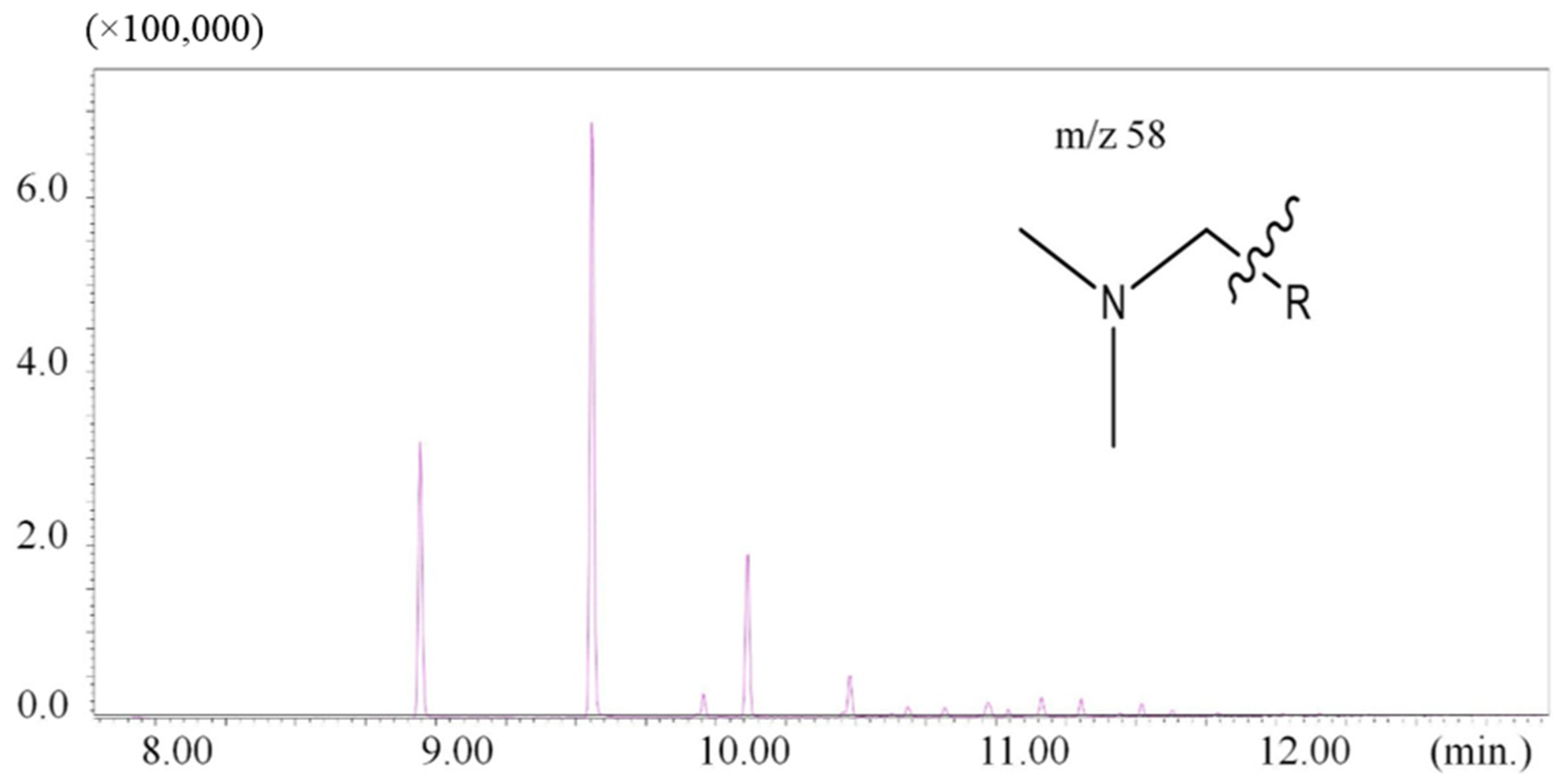
3.2. Organic Compounds Identified in Wastewater Samples
| Retention Time (min) | m/z | Compound | CAS | Samples Contained |
|---|---|---|---|---|
| 1.58 | 50 | Methyl Chloride | 74-87-3 | 1 |
| 1.97 | 76 | Carbon Disulfide | 75-15-0 | 1,3 |
| 4.54 | 91 | Toluene | 108-88-3 | 3 |
| 6.02 | 91 | o-Xylene | 95-47-6 | 3 |
| 6.10 | 57 | 2-Butoxyethanol | 111-76-2 | 3 |
| 8.94 | 58 | N-dodecyl-N,N-dimethylamine | - | 1 |
| 9.56 | 58 | N-tetradecyl-N,N-dimethylamine | - | 1 |
| 10.50 | 107 | Bisphenol F Isomer | - | 1 |
| 10.68 | 107 | Bisphenol F Isomer | - | 1 |
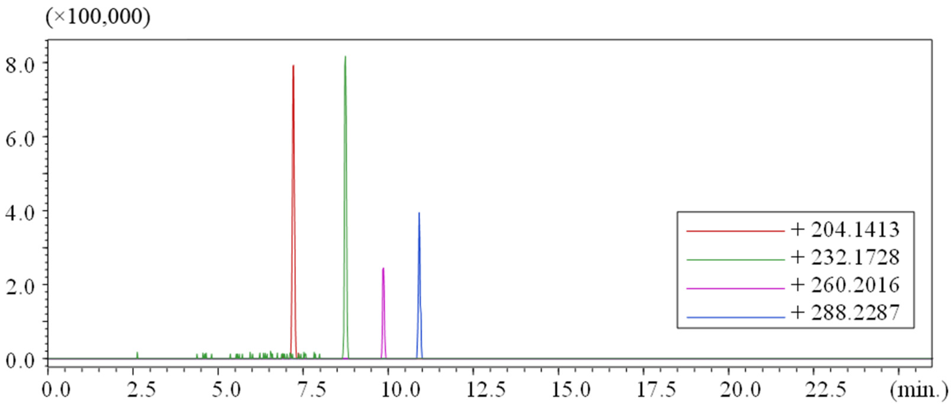
| R.T. (min) | Measured (M + H)+ m/z | Chemical Formula (M) | Error (ppm) |
|---|---|---|---|
| 7.20 | 204.1655 | C10H21NO3 | 26.6 |
| 8.70 | 232.1932 | C12H25NO3 | 7.8 |
| 9.78 | 260.2239 | C14H29NO3 | 4.6 |
| 10.87 | 288.2557 | C16H33NO3 | 5.9 |


3.3. Comparison of Results to Other Studies
4. Conclusions
Acknowledgments
Author Contributions
Conflicts of Interest
References
- Bomgardner, M.M. Cleaner Fracking. Chem. Eng. News. 2012, 90, pp. 13–16. Available online: http://cen.acs.org/content/dam/cen/static/pdfs/Article_Assets/90/09042-cover.pdf (accessed on 22 December 2014).
- Texas RRC. Hydraulic Fracturing. Available online: http://www.webcitation.org/6VSV528rP (accessed on 9 January 2015).
- Orem, W.; Tatu, C.; Varonka, M.; Lerch, H.; Bates, A.; Engle, M.; Crosby, L.; McIntosh, J. Organic substances in produced and formation water from unconventional natural gas extraction in coal and shale. Int. J. Coal Geol. 2014, 126, 20–31. [Google Scholar] [CrossRef]
- Clark, C.E.; Veil, J.A. Produced Water Volumes and Management Practices in the United States; United States Department of Energy,Argonne National Laboratory: DuPage County, IL, USA, 2009. [Google Scholar]
- Frohlich, C. Two-year survey comparing earthquake activity and injection-well locations in the Barnett Shale, Texas. Proc. Natl. Acad. Sci. USA 2012, 109, 13934–13938. [Google Scholar] [CrossRef] [PubMed]
- Hudak, P.F.; Wachal, D.J. Effects of brine injection wells, dry holes, and plugged oil/gas wells on chloride, bromide, and barium concentrations in the Gulf Coast Aquifer, southeast Texas, USA. Environ. Int. 2001, 26, 497–503. [Google Scholar] [CrossRef] [PubMed]
- Vidic, R.D.; Brantley, S.L.; Vandenbossche, J.M.; Yoxtheimer, D.; Abad, J.D. Impact of Shale Gas Development on Regional Water Quality. Science 2013, 340, 826–835. [Google Scholar] [CrossRef]
- Nicot, J.; Scanlon, B.R.; Reedy, R.C.; Costley, R.A. Source and Fate of Hydraulic Fracturing Water in the Barnett Shale: A Historical Perspective. Environ. Sci. Technol. 2014, 48, 2464–2471. [Google Scholar] [PubMed]
- Thiel, G.P.; Tow, E.W.; Banchik, L.D.; Chung, H.W.; Lienhard, J.H. Energy consumption in desalinating produced water from shale oil and gas extraction. Desalination 2015. [Google Scholar] [CrossRef]
- Maguire-Boyle, S.J.; Barron, A.R. Organic compounds in produced waters from shale gas wells. Environ. Sci. Process. Impacts 2014, 16, 2237–2248. [Google Scholar] [CrossRef] [PubMed]
- Thurman, E.M.; Ferrer, I.; Blotevogel, J.; Borch, T. Analysis of Hydraulic Fracturing Flowback and Produced Waters Using Accurate Mass: Identification of Ethoxylated Surfactants. Anal. Chem. 2014, 86, 9653–9661. [Google Scholar] [CrossRef] [PubMed]
- Harkness, J.S.; Dwyer, G.S.; Warner, N.R.; Parker, K.M.; Mitch, W.A.; Vengosh, A. Iodide, Bromide, and Ammonium in Hydraulic Fracturing and Oil and Gas Wastewaters: Environmental Implications. Environ. Sci. Technol. 2015, 49, 1955–1963. [Google Scholar] [CrossRef] [PubMed]
- Lester, Y.; Ferrer, I.; Thurman, E.M.; Sitterley, K.A.; Korak, J.A.; Aiken, G.; Linden, K.G. Characterization of hydraulic fracturing flowback water in Colorado: Implications for water treatment. Sci. Total Environ. 2015, 512–513, 637–644. [Google Scholar] [CrossRef] [PubMed]
- FracFocus Chemical Disclosure Registry. Available online: Fracfocus.org (accessed on 23 January 2015).
- Fontenot, B.E.; Hunt, L.R.; Hildenbrand, Z.L.; Carlton, D.C.; Oka, H.; Walton, J.; Hopkins, D.; Osorio, A.; Bjorndal, B.; Hu, Q.H.; et al. An Evaluation of Water Quality in Private Drinking Water Wells Near Natural Gas Extraction Sites in the Barnett Shale Formation. Environ. Sci. Technol. 2013, 47, 10032–10040. [Google Scholar] [CrossRef] [PubMed]
- Alley, B.; Beebe, A.; Rodgers, J., Jr.; Castle, J.W. Chemical and physical characterization of produced waters from conventional and unconventional fossil fuel resources. Chemosphere 2011, 85, 74–82. [Google Scholar] [CrossRef] [PubMed]
- McLafferty, F.W. Interpretation of Mass Spectra, 3rd ed.; University Science Books: Mill Valley, CA, USA, 1980; pp. 218–221. [Google Scholar]
© 2015 by the authors; licensee MDPI, Basel, Switzerland. This article is an open access article distributed under the terms and conditions of the Creative Commons Attribution license (http://creativecommons.org/licenses/by/4.0/).
Share and Cite
Thacker, J.B.; Carlton, D.D., Jr.; Hildenbrand, Z.L.; Kadjo, A.F.; Schug, K.A. Chemical Analysis of Wastewater from Unconventional Drilling Operations. Water 2015, 7, 1568-1579. https://doi.org/10.3390/w7041568
Thacker JB, Carlton DD Jr., Hildenbrand ZL, Kadjo AF, Schug KA. Chemical Analysis of Wastewater from Unconventional Drilling Operations. Water. 2015; 7(4):1568-1579. https://doi.org/10.3390/w7041568
Chicago/Turabian StyleThacker, Jonathan B., Doug D. Carlton, Jr., Zacariah L. Hildenbrand, Akinde F. Kadjo, and Kevin A. Schug. 2015. "Chemical Analysis of Wastewater from Unconventional Drilling Operations" Water 7, no. 4: 1568-1579. https://doi.org/10.3390/w7041568
APA StyleThacker, J. B., Carlton, D. D., Jr., Hildenbrand, Z. L., Kadjo, A. F., & Schug, K. A. (2015). Chemical Analysis of Wastewater from Unconventional Drilling Operations. Water, 7(4), 1568-1579. https://doi.org/10.3390/w7041568