3.1. Building Drag Resistance
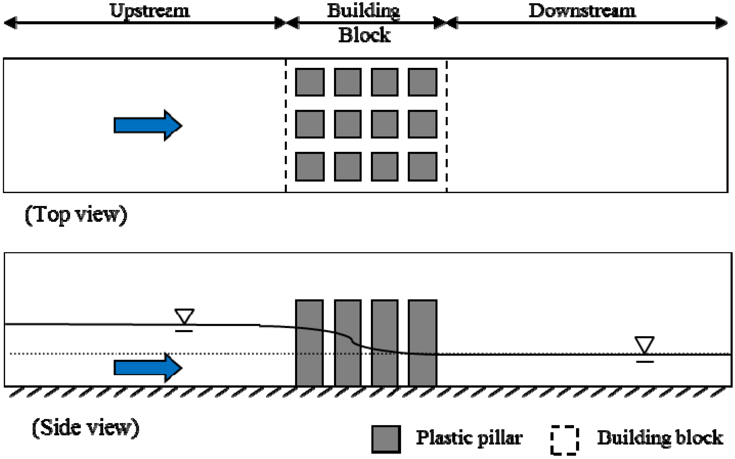
The flume was built in a smooth boundary channel so that the surface resistance is small compared with the drag resistance in the experiment. Assuming that the effect of surface resistance can be neglected, the experimental slope of the energy-grade line (
![]()
) contributed by drag resistance is expressed as follows:
where
Y1 and
Y2 are the upstream and downstream water depth; whereas Δ
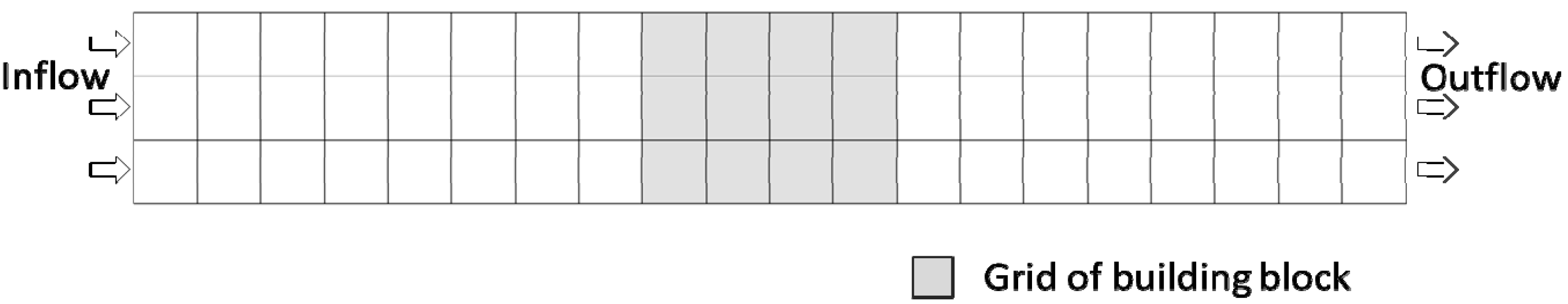
x is the length of the building block (1.33 m).
From Manning Equation, the experimental slope of the energy-grade line (
![]()
) due to the shape resistance can be used to obtain the experimental roughness,
n", which represents the building drag resistance:
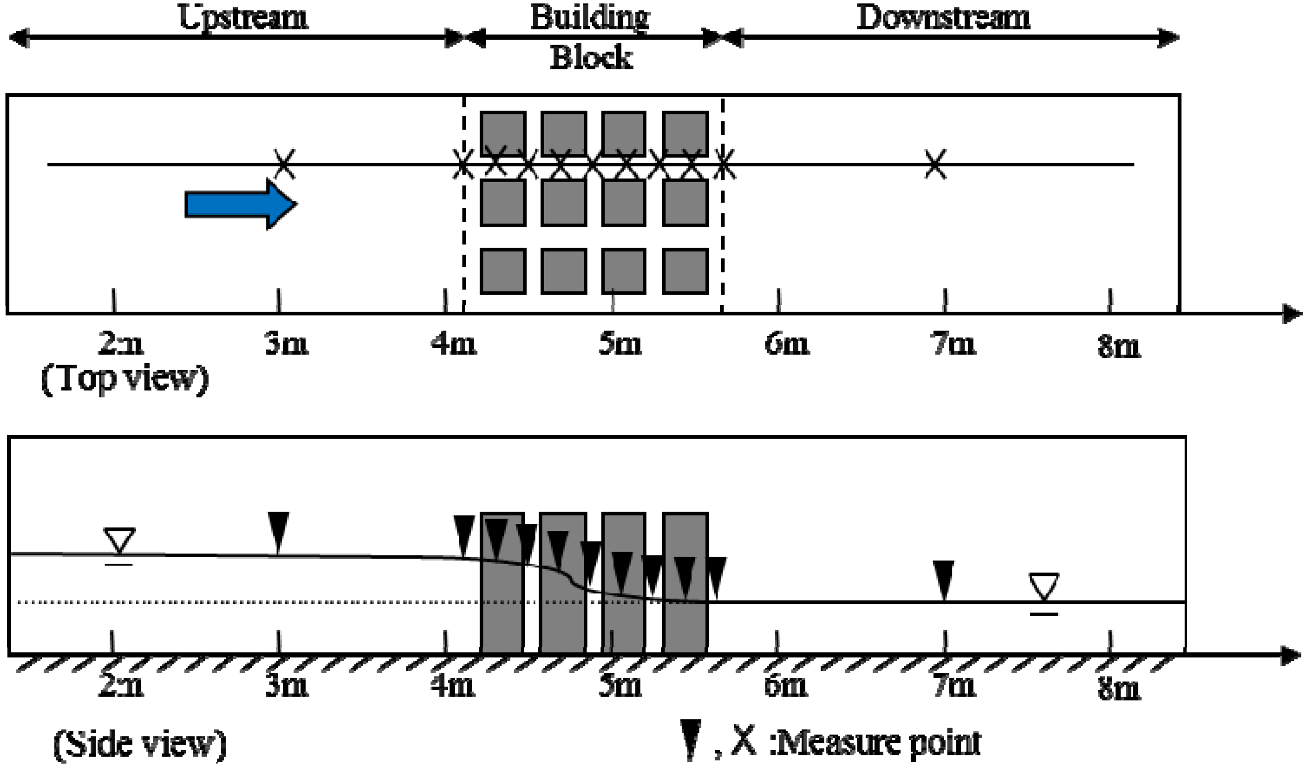
Considering the oscillation of water depth in the building block, d is defined as the mean value of upstream and downstream depth, i.e., d = (Y1 + Y2)/2, and V is also the mean value, V = (V1 + V2)/2.
Table 1 shows the mean water depth and velocity of each setting. While the upstream water depth
Y1 increases with BCR significantly, the downstream depth
Y2 remains unchanged. The results show that the downstream water depths remain unchanged, and there are only a few differences in downstream velocities. It indicates that the wave celerity is larger than the flow velocity in subcritical flow,
i.e., the wave travels in upstream direction and induces the backwater effect.
Table 1.
Water depths (unit: cm) and velocities (unit: cm/s) in different building coverage ratio (BCRs).
Table 1.
Water depths (unit: cm) and velocities (unit: cm/s) in different building coverage ratio (BCRs).
| BCR (α0) | 0.00 | 0.04 | 0.16 | 0.25 | 0.36 | 0.49 | 0.64 |
|---|
| Upstream mean water depth, Y1 | 8.50 | 8.80 | 9.00 | 9.30 | 9.55 | 10.20 | 11.70 |
| Downstream mean water depth, Y2 | 8.50 | 8.50 | 8.50 | 8.50 | 8.50 | 8.50 | 8.50 |
| Upstream mean water velocity, V1 | 13.74 | 13.33 | 13.25 | 12.59 | 12.29 | 11.53 | 9.85 |
| Downstream mean water velocity, V2 | 13.74 | 13.60 | 13.60 | 13.61 | 13.62 | 13.65 | 13.84 |
We can calculate
V,
d,
![]()
under different BCR values shown in
Table 2, and obtain
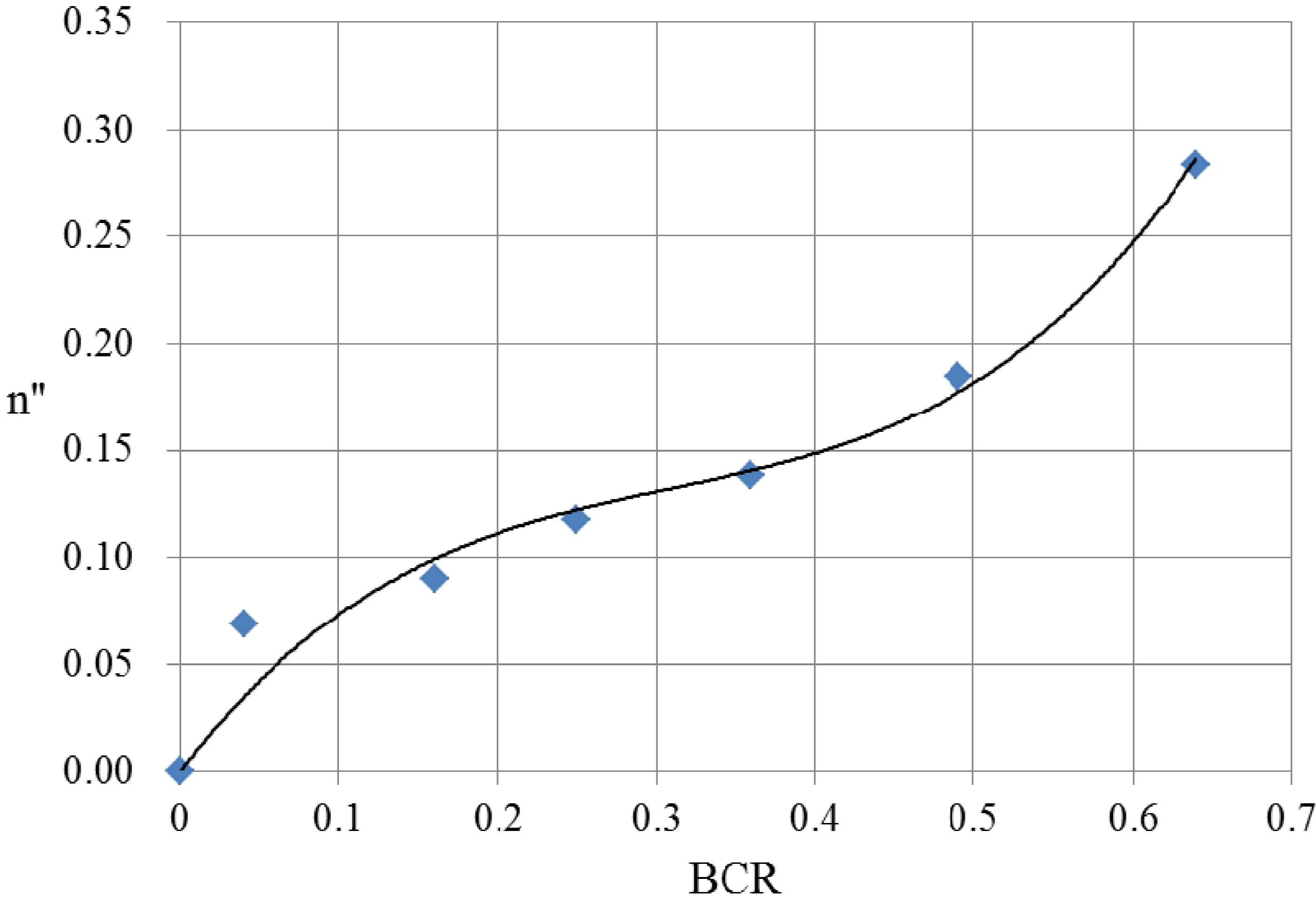
n" from Equation (12). The relationship between BCR and
n" is plotted in
Figure 6. By polynomial regression we can obtain the experimental roughness
n" as below.
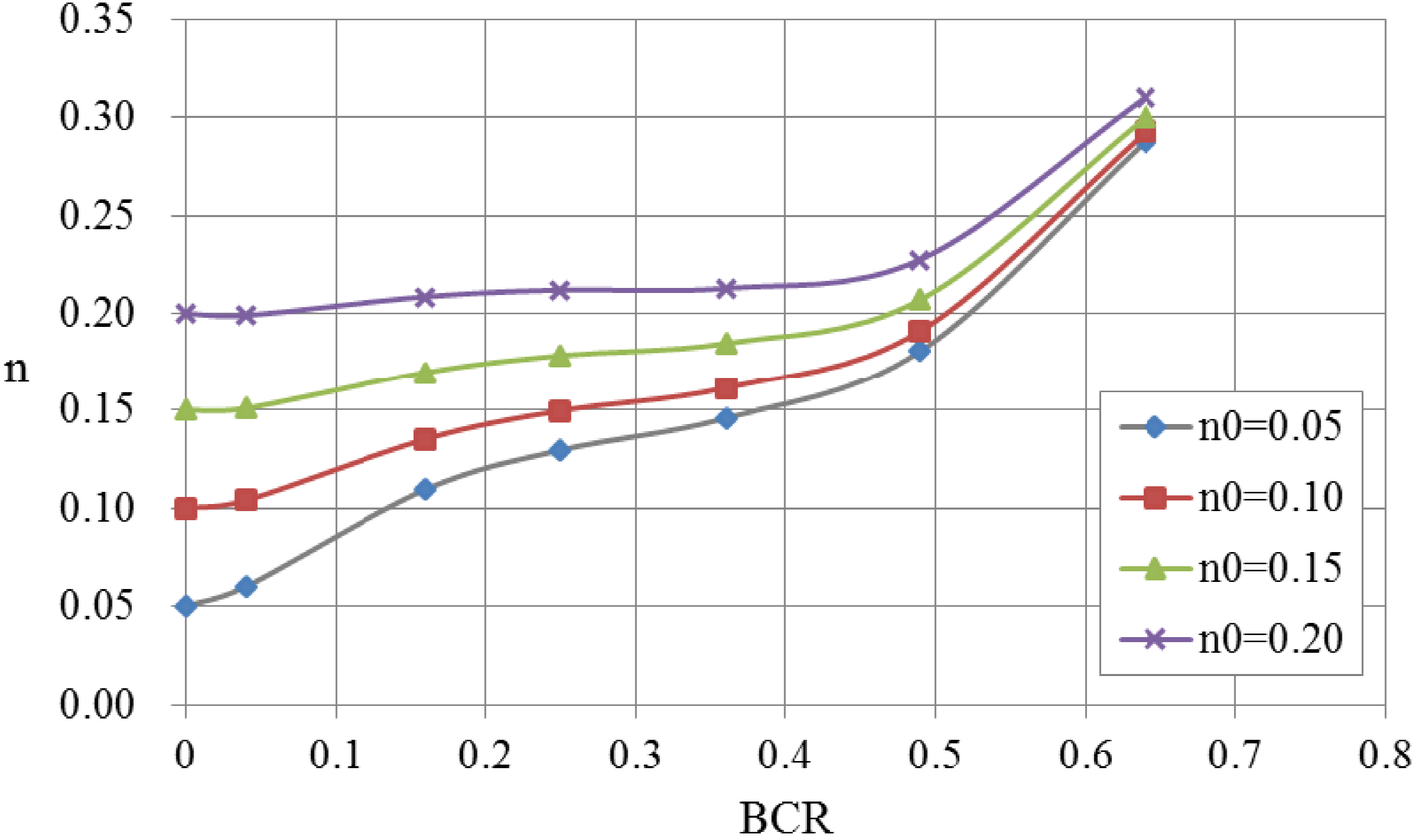
According to Equations (10) and (13), the roughness corresponding to the blockage effect can be obtained.
Different value of
n0 and BCR were inputted into Equation (14) to observe the relationship of BCR and
n, as shown in
Figure 7. It can be seen that roughness generally increased with BCR. For example, roughness
n increased mildly with BCR, but rapidly when BCR is greater than 0.45. The trend shows that surface resistance dominates the change of roughness when BCR is small. With increasing BCR, first roughness increased markedly and then, when BCR is close to 0.64, it remains approximately constant close to the value of 0.3. Further, this analysis indicates that BCR is the main factor influencing roughness for larger values of BCR.
Table 2.
Water depths in different BCRs (unit: cm).
Table 2.
Water depths in different BCRs (unit: cm).
| BCR (α0) | 0.00 | 0.04 | 0.16 | 0.25 | 0.36 | 0.49 | 0.64 |
|---|
| V | 13.74 | 13.46 | 13.43 | 13.10 | 12.95 | 12.59 | 11.85 |
| d | 8.50 | 8.65 | 8.75 | 8.90 | 9.03 | 9.35 | 10.10 |
![]() | 0.00000 | 0.00226 | 0.00376 | 0.00602 | 0.00789 | 0.01278 | 0.02406 |
| n" | 0.000 | 0.069 | 0.090 | 0.118 | 0.138 | 0.185 | 0.284 |
Figure 6.
Relationship between n" and BCR.
Figure 6.
Relationship between n" and BCR.
Figure 7.
Relationship between n and BCR under different n0.
Figure 7.
Relationship between n and BCR under different n0.
3.2. Scale Adjustment
Due to scale differences between the experiment and urban areas, roughness corresponding to the blockage effect in Equation (14) was modified by scale adjustment to allow applications in urban inundation modeling.
The ratio of simulation roughness of the urban area scale to the experimental scale (
![]()
) can be expressed as:
where
Sfr is the ratio of the slope of energy-grade line,
dr is the ratio of water depth (
dr =
d/0.085), and
Vr is the ratio of flow velocity.
While water flow passes through buildings, systematic and sudden widening and narrowing may occur. The slope of the energy-grade line in the longitudinal direction of the flow can be determined by Borda’s formula [
10]
where the length
L is the spatial typical scale of the widening and narrowing (
i.e., the grid side), and
k is the head loss coefficient.
Thus the ratio of the slope of energy-grade line is:
where
Lr is the ratio of the simulation grid cell size to the experimental grid cell size (
Lr = Δ
x/0.33).
By substituting
Sfr of Equation (17) into Equation (15), the ratio of roughness
![]()
can be obtained.
Experimental roughness
n" in Equation (14) has to be modified with
![]()
to represent the roughness in the urban inundation simulation.
3.4. Model Application
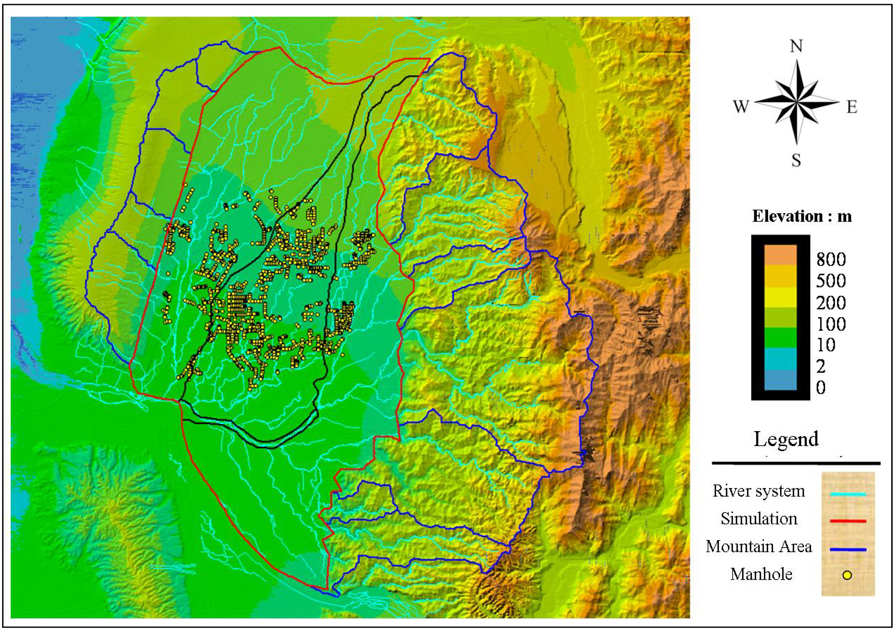
Taichung City in middle Taiwan has Dakeng Mountain on the east side and Dadu in the west side.
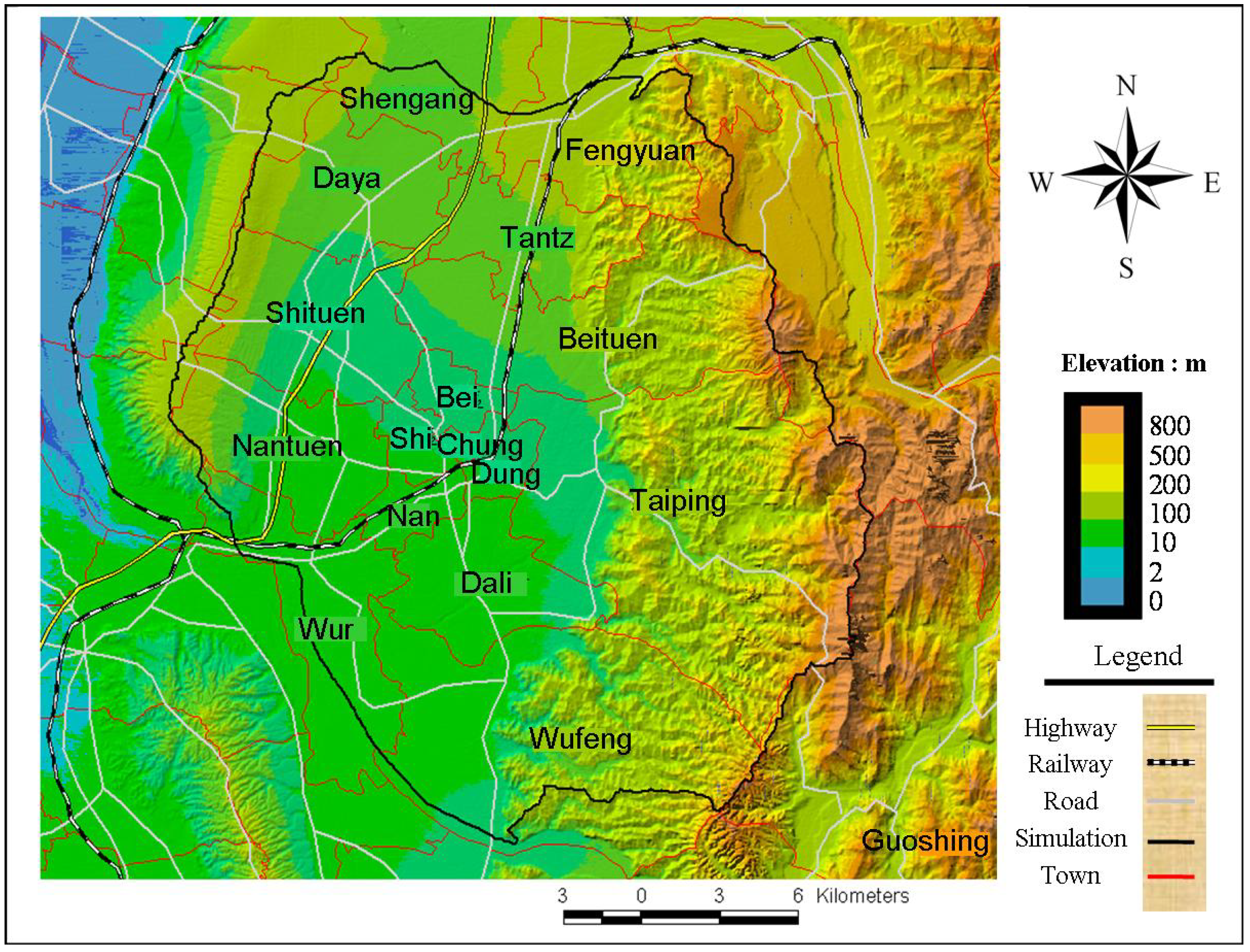
Figure 16 shows the topography and administrative borders of Taichung City. Taichung is a basin with the lowland in its southwest area. In the south, there are the Dali River and Wu River. The railway goes through the downtown, and the highway gets across the city along the Fazih River. The convenient traffic network consists of several importantly expressed ways, which encourage the centralization of the urban population.
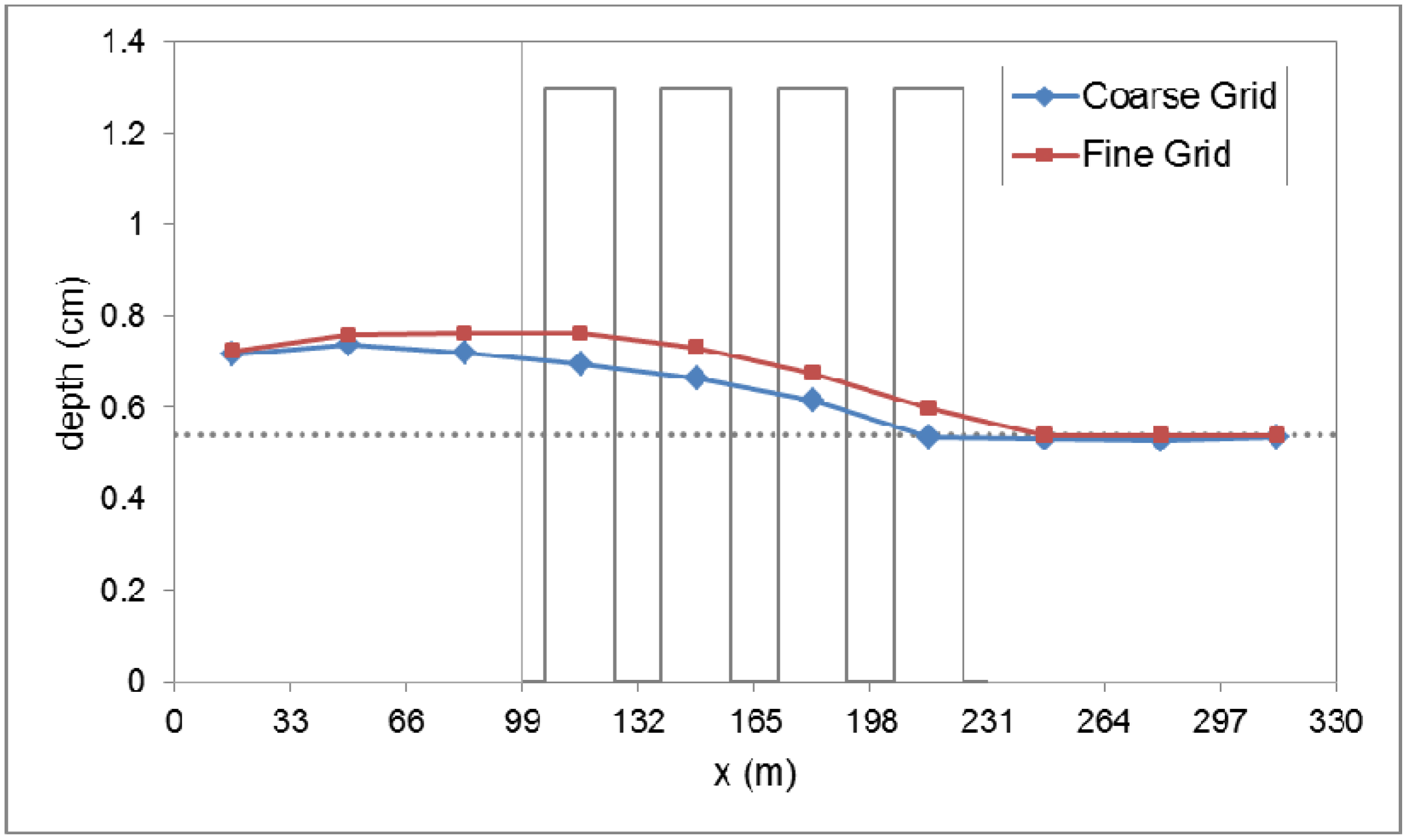
Figure 13.
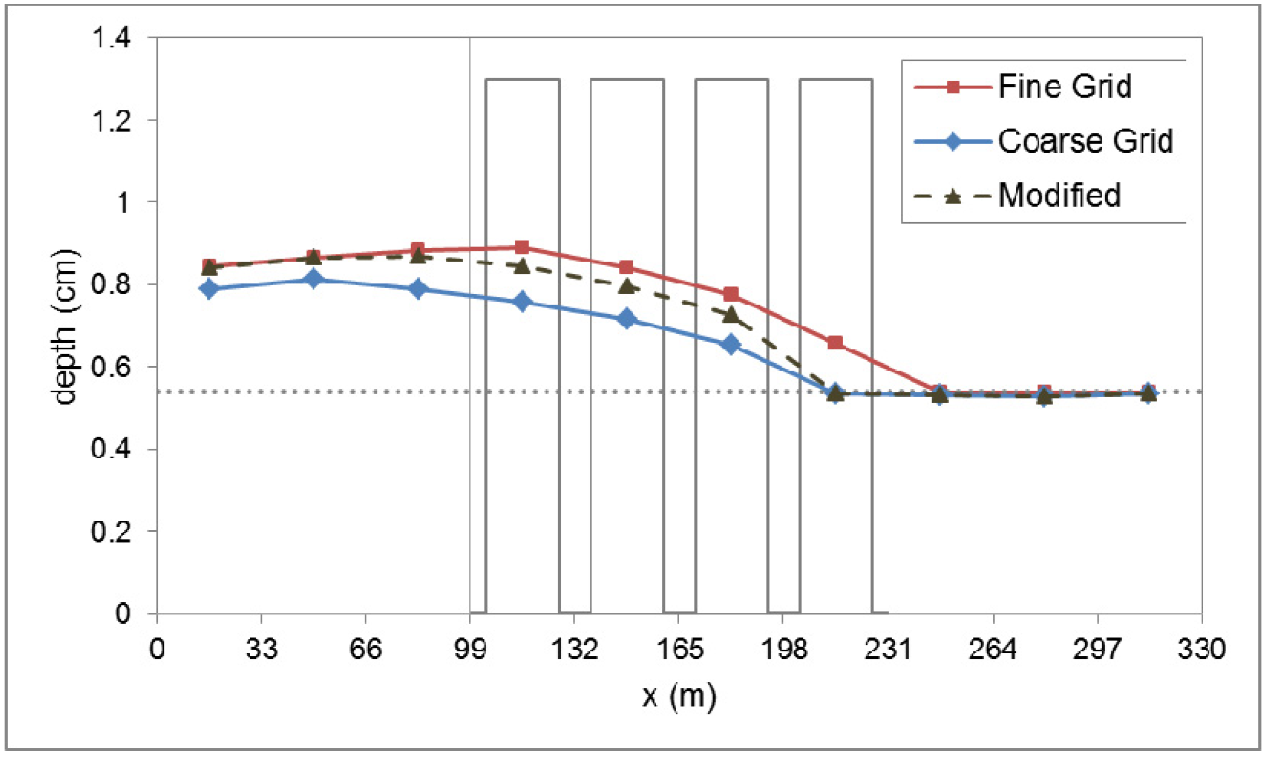
Water profile of experiment and simulation results in real scale (α0 = 0.36).
Figure 13.
Water profile of experiment and simulation results in real scale (α0 = 0.36).
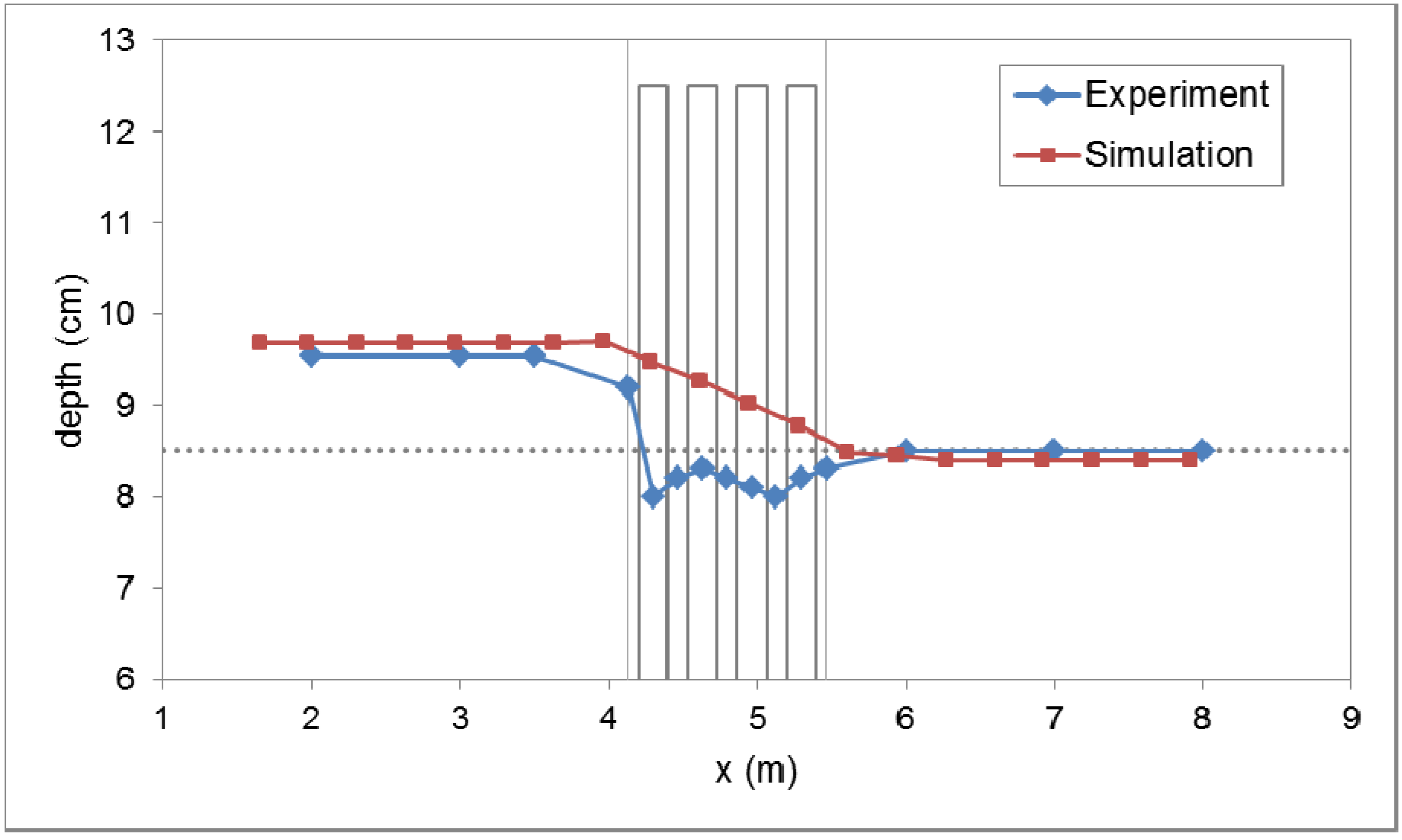
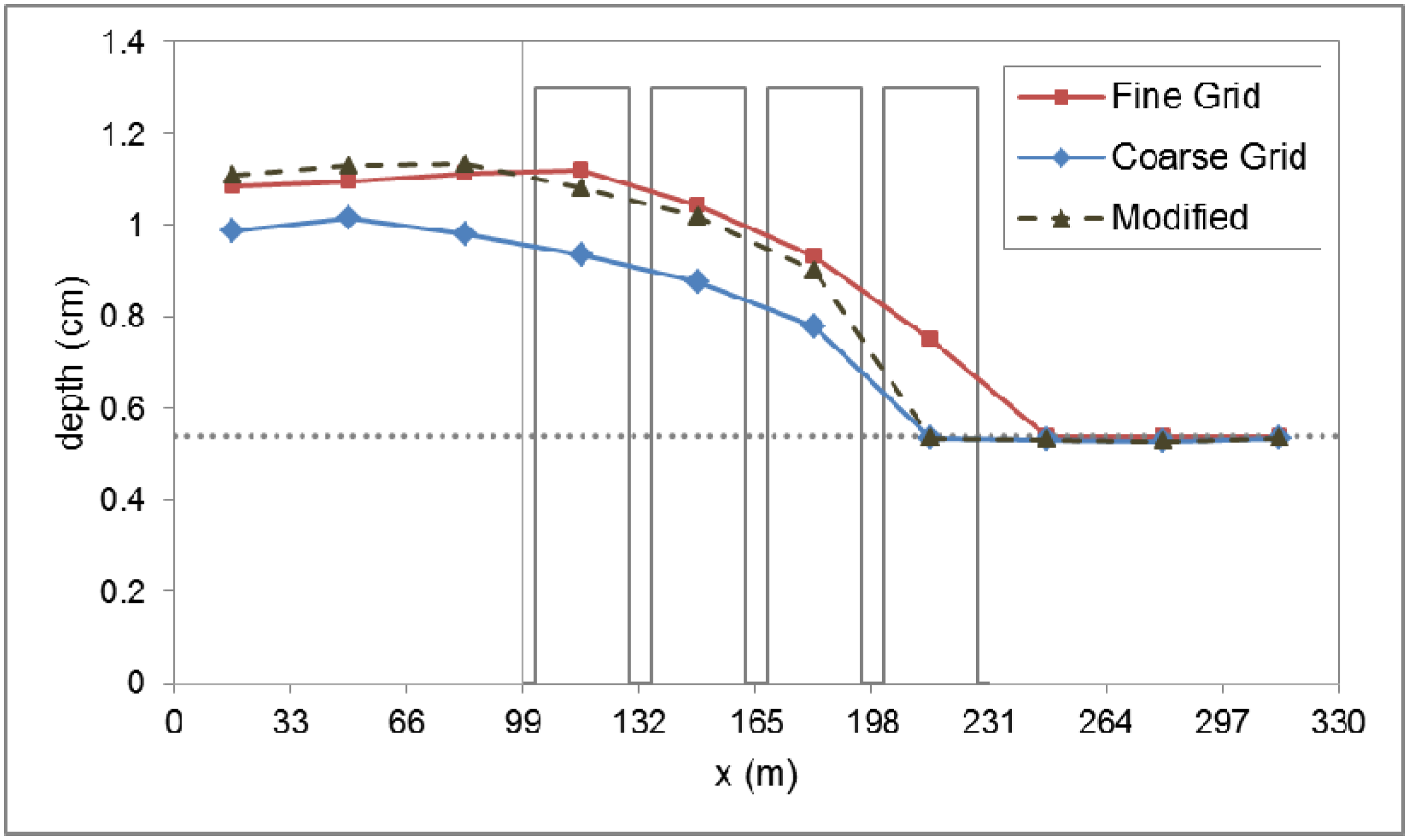
Figure 14.
Water profile of experiment and simulation results in real scale (α0 = 0.49).
Figure 14.
Water profile of experiment and simulation results in real scale (α0 = 0.49).
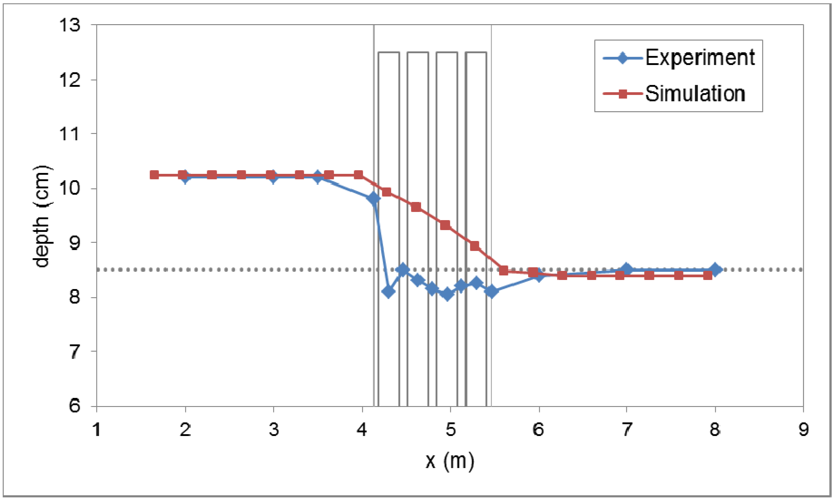
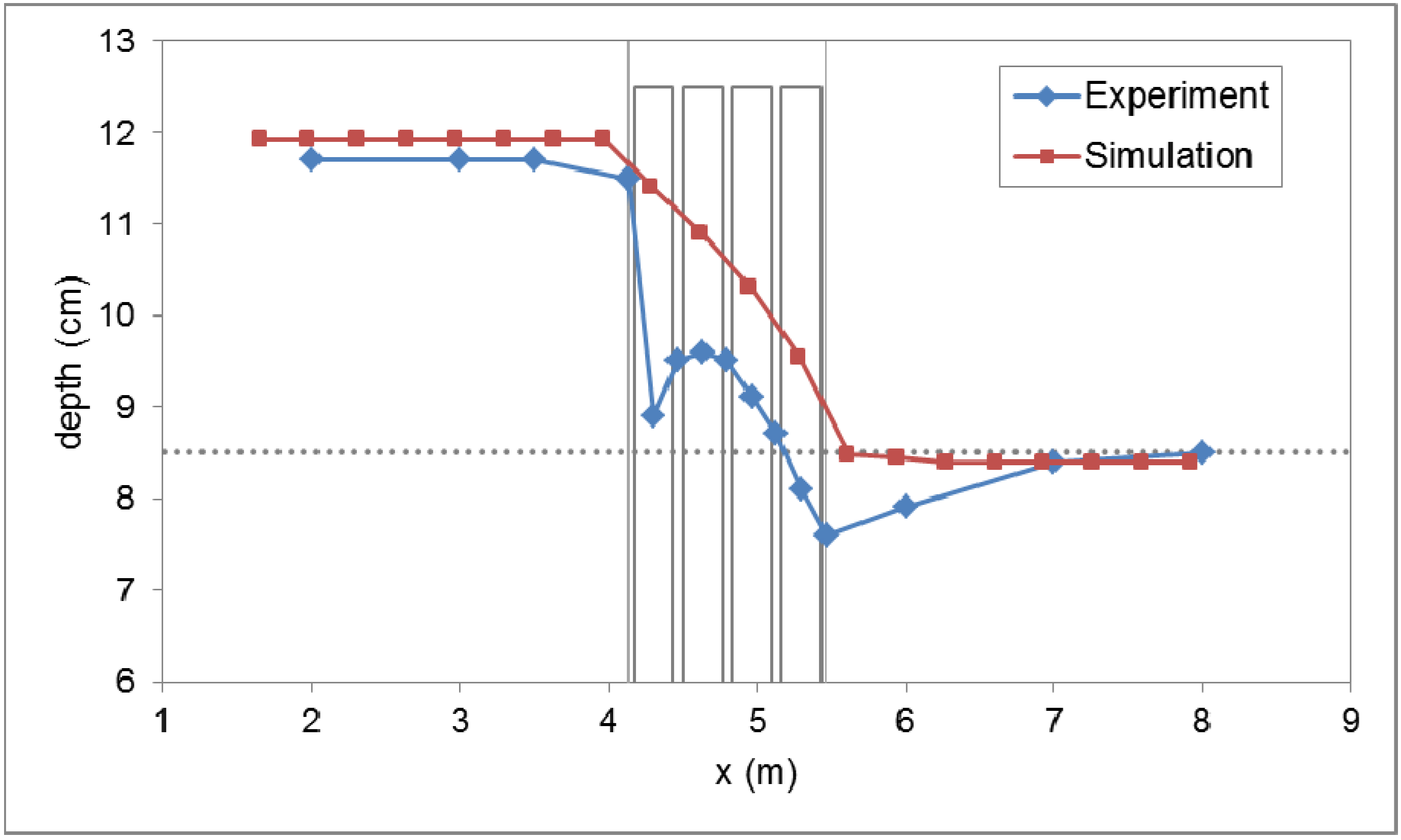
Figure 15.
Water profile of experiment and simulation results in real scale (α0 = 0.64).
Figure 15.
Water profile of experiment and simulation results in real scale (α0 = 0.64).
Figure 16.
Elevation, water system, and sewer manholes of Taichung city.
Figure 16.
Elevation, water system, and sewer manholes of Taichung city.
There are 174 sewers and 2018 manholes in Taichung City.
Figure 17 shows the distribution of the sewer manholes. In the sewer system, the pipe diameter is 600 mm. From higher to lower pipes, the diameter increases up to 2000 mm.
Figure 17.
Distribution of the sewer manholes of Taichung city.
Figure 17.
Distribution of the sewer manholes of Taichung city.
Typhoon Kalmaegi in 2008 was adopted for model application. Typhoon Kalmaegi intruded Taichung on 17 July 2008.
Table 5 shows the total amount and peak intensity of 24 h rainfall from 17 July 2008, 23:00, to 18 July 2008, 22:00. The peak intensity of most rain gauges exceeded the design standard (73 mm/h) of the sewer system in Taichung City.
Table 5.
Total amount and peak intensity of rainfall of Typhoon Kalmaegi in Taichung City.
Table 5.
Total amount and peak intensity of rainfall of Typhoon Kalmaegi in Taichung City.
| Rain gauge | Total rainfall (mm) | Peak intensity (mm/h) |
|---|
| Taichung | 478.9 | 120.0 |
| Dadu | 363.0 | 79.0 |
| Shhigang | 341.0 | 74.5 |
| Dakeng | 607.0 | 149.0 |
| Chungchulin | 567.0 | 91.0 |
| Tonlin | 409.5 | 82.5 |
| Shengang | 225.5 | 49.5 |
| Fenyuan | 377.5 | 78.5 |
| Changhua | 248.0 | 52.0 |
| Caotun | 295.0 | 71.0 |
The HEC-1 Model developed by the U.S. Army Corps of Engineers [
15] was used to calculate runoffs of the upstream catchments that in turn can be used as lateral inflows in the 2D inundation model. The Storm Water Management Model (SWMM) [
16] was adopted to solve the sewer system in Taichung City. The discharges drained by pumping stations are considered as the lateral outflows of the model, and the surcharges of manholes are regarded as point sources in the model [
17].
We compared two cases for reflecting building blockages in urban flood modeling with 80 m × 80 m cells. Case 1 only adopted the bare terrain elevation without roughness adjustment, and it is the traditional approach in urban flood modeling. The original Manning’s roughness of each grid cell was assumed according the land-use type of each cell and classified into the following three categories: 0.1 (waterway), 0.13 (agricultural, residential and traffic uses), and 0.20 (commercial and industrial uses). In Case 2, BCR values and adjusted roughness were used to represent the blockage effect. The BCR values were calculated from the occupied area of buildings in each cell. The Manning’s roughness of each cell was modified according to Equation (19) during the simulation. The average BCR values of all districts listed in
Table 6 are mean BCR values of all the cells located in the districts.
Table 6.
Inundation area of Taichung City (unit: ha).
Table 6.
Inundation area of Taichung City (unit: ha).
| District | Case 1 | Case 2 | Average BCR |
|---|
| Situn | 638.08 | 705.28 | 0.22 |
| Nantun | 556.80 | 566.40 | 0.20 |
| Beitun | 424.32 | 550.40 | 0.26 |
| East | 186.24 | 255.36 | 0.36 |
| South | 283.52 | 305.92 | 0.34 |
| West | 222.72 | 246.30 | 0.41 |
| North | 166.40 | 213.76 | 0.43 |
| Central | 27.52 | 33.92 | 0.53 |
| Total | 2505.60 | 2877.34 | |
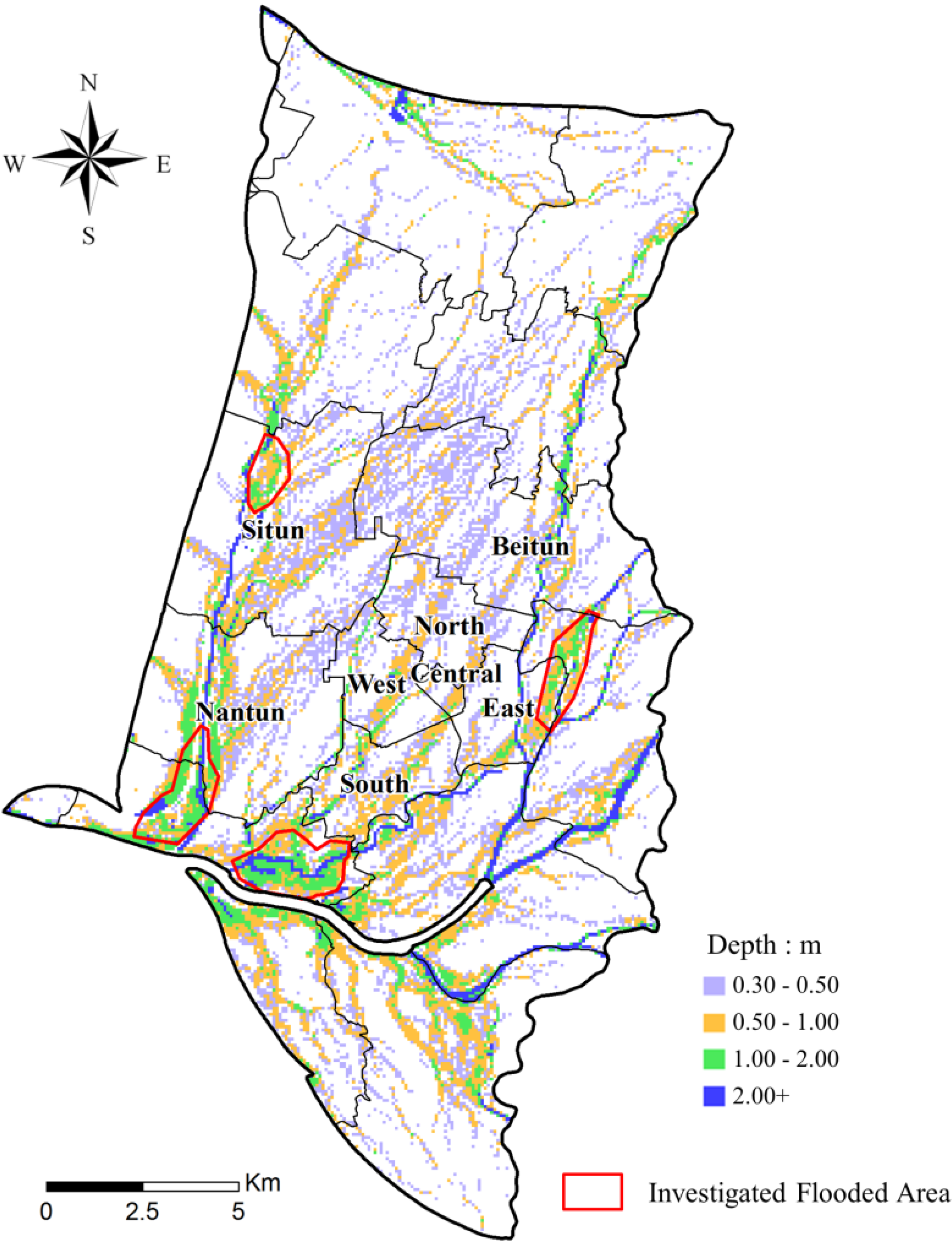
Figure 18 shows the simulated flooded area of Case 2 and investigated flooded area for Typhoon Kalmaegi surveyed by Taichung City Government. The torrential rainfall caused serious flood damage in Taichung city. The severe inundated area in Situn, Nantun, South, and East district can be simulated from the inundation model. The total inundation area was the summation of water depth above 0.5 m and shown in
Table 6. It can be found that according to the modifications of the surface roughness value with BCR, the inundated area was obviously increased from 2506 to 2877 ha due to densely distributed buildings. The inundation area of all districts had the same trend. The inundation areas of each district are shown in
Table 7. It is noted that the Nantun district had the smallest average BCR and the inundated area increased from 556.8 ha to 566.4 ha, which is an increase of about 1.7%. The Central district had the highest BCR and the increased ratio of inundated area reached 23.26%, which means that the water spread wider due to the existence of buildings. These results indicated that the blockage effect was more significant when the building occupancy on the surface was higher. From the results we can conclude that flood area increased due to the blockage effect of buildings, which indicates the flash flood in urban area will induce the severe inundation area and cause higher impact.
Figure 18.
Simulated and investigated flooded areas of Typhoon Kalmaegi with building blockage effect (Case 2).
Figure 18.
Simulated and investigated flooded areas of Typhoon Kalmaegi with building blockage effect (Case 2).
Table 7.
Inundation area of each districts of Taichung City (unit: ha).
Table 7.
Inundation area of each districts of Taichung City (unit: ha).
| Depth (m) | Situn | Nantun | Beitun | East |
|---|
| Case 1 | Case 2 | Case 1 | Case 2 | Case 1 | Case 2 | Case 1 | Case 2 |
|---|
| 0.5–1.0 | 453.76 | 500.48 | 339.20 | 349.44 | 345.60 | 437.76 | 131.84 | 139.52 |
| 1.0–2.0 | 126.08 | 144.00 | 176.00 | 176.00 | 32.64 | 66.56 | 52.48 | 89.60 |
| 2.0–3.0 | 34.56 | 36.48 | 8.96 | 8.32 | 28.80 | 26.88 | 1.28 | 11.52 |
| above 3.0 | 23.68 | 24.32 | 32.64 | 32.64 | 17.28 | 19.20 | 0.64 | 14.72 |
| Total | 638.08 | 705.28 | 556.80 | 566.40 | 424.32 | 550.40 | 186.24 | 255.36 |
| Depth (m) | South | West | North | Central |
| Case 1 | Case 2 | Case 1 | Case 2 | Case 1 | Case 2 | Case 1 | Case 2 |
| 0.5–1.0 | 201.60 | 216.32 | 128.00 | 140.47 | 159.36 | 198.40 | 22.40 | 20.48 |
| 1.0–2.0 | 61.44 | 69.12 | 69.76 | 72.23 | 6.40 | 14.72 | 5.12 | 13.44 |
| 2.0–3.0 | 18.56 | 17.92 | 10.24 | 17.28 | 0.64 | 0.64 | 0.00 | 0.00 |
| above 3.0 | 1.92 | 2.56 | 14.72 | 16.32 | 0.00 | 0.00 | 0.00 | 0.00 |
| Total | 283.52 | 305.92 | 222.72 | 246.30 | 166.40 | 213.76 | 27.52 | 33.92 |


 , where
  and n0 is Manning’s roughness without considering the building effect, and substituting τw in Equation (6), the reduced resistance force becomes as follows:


 ) contributed by drag resistance is expressed as follows:


 ) can be expressed as: