Identifying Major Factors Affecting Groundwater Change in the North China Plain with Grey Relational Analysis

Abstract

The North China Plain (NCP) is facing a water crisis under the dual impact of natural and anthropogenic factors. Groundwater levels have declined continuously since 1960, causing a series of environmental problems that have restricted sustainable development in the region. In the present study, we first utilized a previously developed 3D groundwater model to determine changes in groundwater level in the region over the past 50 years (1961–2010). We then applied grey relational analysis (GRA) to identify and ordinate major factors that have contributed to these changes. The results show an overall decreasing trend in groundwater levels in this region over the past 50 years and an increase in the water table depth at a rate of approximately 0.36 m/a. Groundwater exploitation showed the most significant correlation with the groundwater table decline, when compared with other factors including precipitation and river leakage. Therefore, human activities should be considered the primary force driving the groundwater level down. The results of this study have implications for developing criteria that consider changes in both climate and socio-economics. Furthermore, since the NCP is one of the most water-scarce and densely populated regions in the world, the analytical approach used in and the insights gained from this study are of international interest.

1. Introduction

Groundwater is directly related to human existence and to the sustainable development of a society, because it plays an important role as a water resource. More than two billion people worldwide depend on groundwater for their daily water supply, and a large proportion of the world’s agricultural and industrial water requirements are supplied by groundwater [1]. Due to an increasing demand for groundwater in response to rapidly growing urban, industrial, and agricultural water requirements, several countries, especially those in arid and semi-arid zones, are experiencing water shortages resulting from the imbalance between demand and supply [2].

Groundwater resources are influenced by both climate change and human activities [3,4]. For example, climate change has resulted in increasing global atmospheric temperatures, and has led to a modified precipitation pattern, which may have a direct impact on groundwater levels [5]. Previous studies investigating the response of groundwater systems to climate change have achieved considerable success [6,7,8]. It has been shown that groundwater systems have undergone changes due to human activities, including groundwater abstraction and reservoir construction. Since 1960, access to pumped wells has caused a rapid worldwide increase in groundwater development for municipal, industrial, and agricultural purposes [9]. The global use of groundwater was estimated to be 750–800 km³/a [10,11].

The combination of climate change and indiscriminate groundwater development has caused a general decline in groundwater levels, resulting in the depletion of groundwater, land subsidence, and saltwater intrusion in deltaic areas [12]. Lower groundwater levels are a threat to the environment and hinder economic development. Excessive groundwater depletion has affected vast regions, including Northwest India, North China, and the Central USA [13]. Thus, it is important to understand the evolution of groundwater systems, and the dual effects of climate change and anthropogenic activities.

The North China Plain (NCP) is an example of an area where groundwater levels have declined continuously since 1960. It is one of the most densely populated regions in the world, with a population of approximately 130 million in an area of about 140,000 km² [14]. As one of the most important social, economic, and agricultural regions in China, the NCP contributes approximately 25% of the total grain yield of China, and groundwater provides 70% of the water supply for this region [15]. As water demand has exceeded the natural renewable supply, many urban and irrigated areas in the NCP have come to experience regular water shortages. The indiscriminate exploitation of groundwater and decreasing precipitation over recent years has caused groundwater levels to continue to decline [16,17] with adverse environmental effects [18,19]. Therefore, it is particularly important to study the change of groundwater in the NCP and to analyze the factors influencing groundwater dynamics.

Groundwater is a complex system from recharge to discharge, and its analysis is often subject to large uncertainty owing to insufficient data. Groundwater can therefore be regarded as a grey system, i.e., one with insufficient information [20]. In the early 1980s, Deng [21] formally introduced the grey system theory to handle uncertainties in small data samples with imprecise information, and this field has expanded to include grey relational analysis (GRA), grey modeling (GM), and prediction theory [20,22]. To date, grey system theory has been applied extensively in many fields, including hydrology, manufacturing, and financial analyses [23,24,25]. For groundwater, Gau et al. [26] used GRA to identify factors for the selection of suitable groundwater recharge sites, using hydrogeological data obtained with a groundwater flow model. Similarly, Du et al. [27] adopted GRA to infer that surface water irrigation and groundwater mining are the main factors driving change in groundwater levels in both highland and lowland areas in the Baojixia Irrigation District. Yeh et al. [28] used grey theory to predict variations in the water level in observation wells on the Pingtung Plain. However, no study to date has used GRA to identify the major factors influencing groundwater levels in the NCP, which faces a water crisis.

In this study, we first apply a previously established 3D groundwater model based on MODFLOW to understand groundwater change since 1960 in the over-exploited area of the NCP. Then, we analyze variations in factors influencing groundwater levels and identify the major factors based on GRA.

2. Study Area and Hydrogeologic Setting

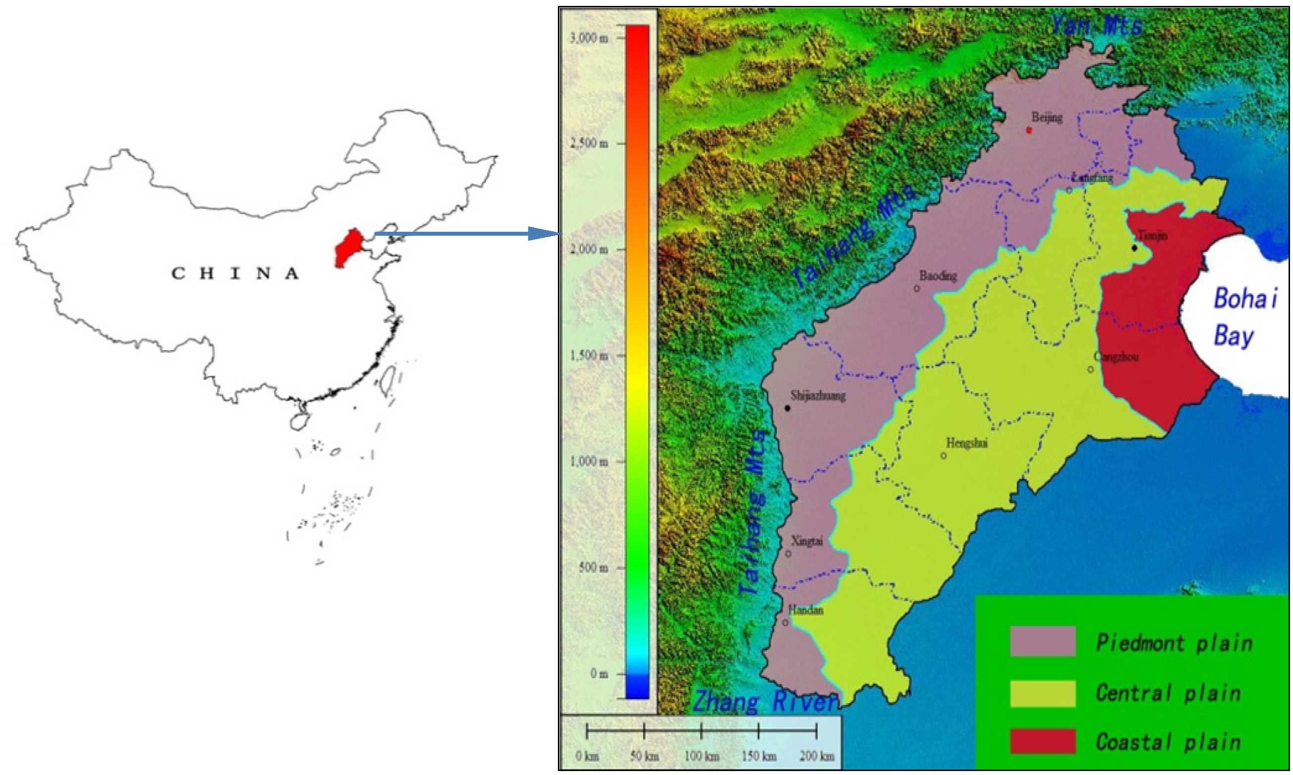
Our study region spans 114.2°–118.1° E and 36.0°–40.6° N, and includes two municipalities (Beijing and Tianjin) and one province (Hebei). We consider Beijing, Tianjin, and Hebei plains as three typical areas with depleted groundwater levels. The study region has an area of 80,592 km² and is bordered by the Taihang and Yan mountains, Bohai Bay, and the Zhang River to the west, north, east, and south, respectively (Figure 1). The landforms are typical of a plain landscape, with elevation less than 100 m. From west to east, the region can be divided into three principal zones: the piedmont, central, and coastal plains. This region experiences a semi-arid continental monsoon climate, with annual average precipitation of approximately 500–600 mm, 75% of which occurs in the summer (i.e., from July to September). Annual water surface evaporation ranges from 1100 to 2000 mm.

Figure 1. Location and topography of study area

Figure 1. Location and topography of study area

The stratigraphy of the study area consists mainly of unconsolidated Quaternary sediments. Based on this stratigraphy, the groundwater system is divided into four aquifer groups [29]; aquifers I and II are combined as shallow aquifers, whereas III and IV are deep aquifers (Figure 2).

Figure 2. Hydrogeological section of the study area [29].

Figure 2. Hydrogeological section of the study area [29].

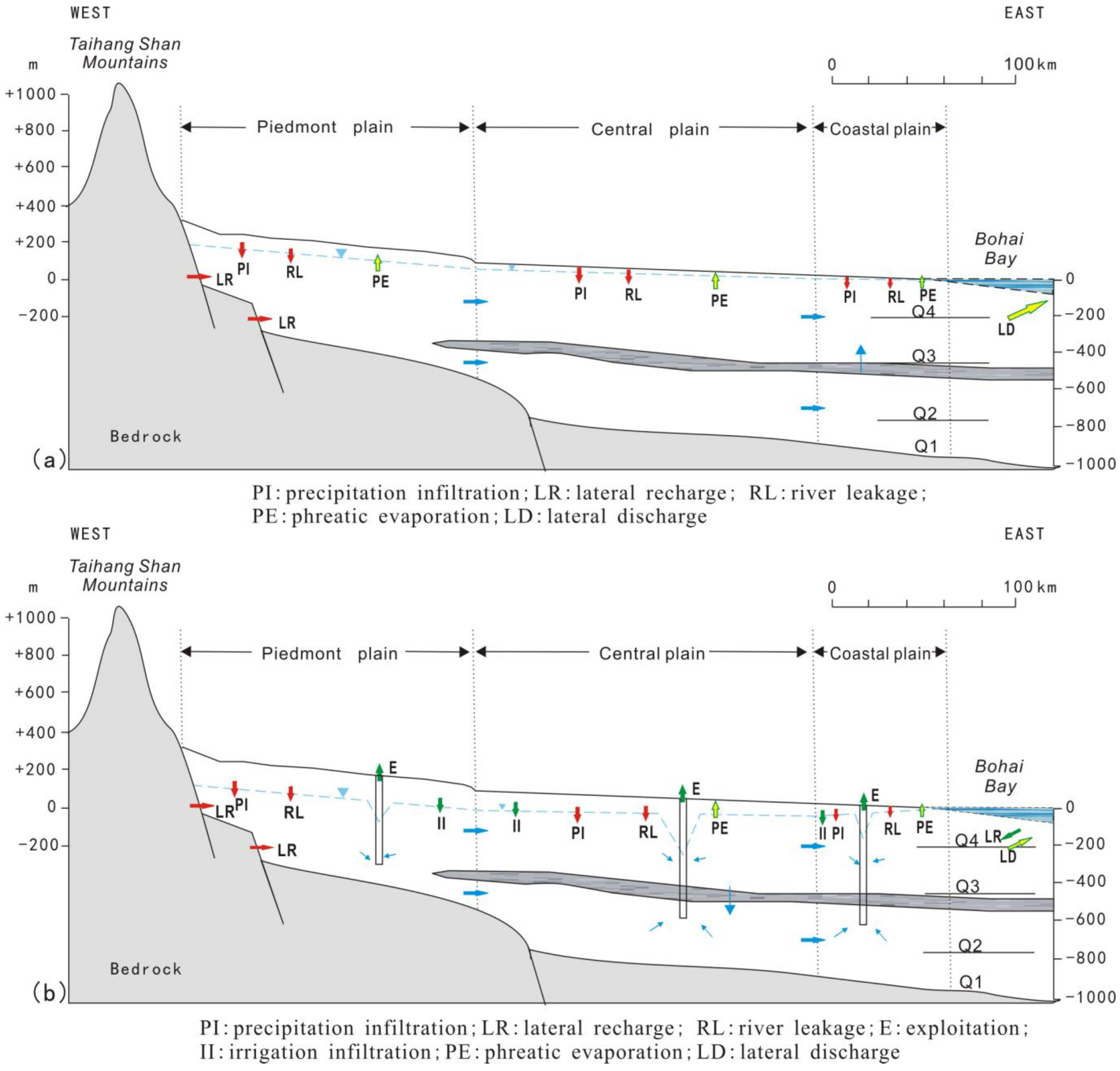
The recharge, runoff, and discharge of the system have changed over the past 50 years influenced by natural climate and human activities (Figure 3). Under natural conditions, recharge resulted primarily from precipitation infiltration, mountainous lateral flow, and river leakage, and discharge was primarily through phreatic evaporation. Groundwater flowed from west to east, and the deep water flowed into the shallow aquifers at the center and east of the plain. At present, irrigation return flow forms an additional recharge source, and exploitation has replaced phreatic evaporation as the main discharge. Groundwater now flows into the center of the cone, with shallow water flowing into the deep aquifers in the center and east of the plain.

Figure 3. Changes in groundwater recharge, runoff, and discharge in the study area (a) in the natural state; and (b) under natural climate and anthropogenic influence.

Figure 3. Changes in groundwater recharge, runoff, and discharge in the study area (a) in the natural state; and (b) under natural climate and anthropogenic influence.

3. Methods

3.1. Groundwater Flow Model

The groundwater flow model is based on MODFLOW (Modular Three-dimensional Finite-difference Ground-water Flow Model) [30], which incorporates a set of stress packages that enable the simulation of external flow stresses, such as those imposed by wells, areal recharge, evapotranspiration, drains, and rivers [31,32]. To apply a groundwater model to a specific site, the conceptual model must be identified [33,34]. Here, we generalized the groundwater flow in the study area as a heterogeneous, anisotropic, transient, and three-dimensional flow system.

The numerical model had 188706 active cells and each grid cell was 2 km × 2 km, based on the hydrogeological conditions and data obtained from the porous aquifers at the study site. The model included three layers: aquifer groups I and II (layer 1); group III (2); and group IV (3). The simulation was run from 1961 to 2010 at a temporal interval of 1 year. The observed field of groundwater in 1959 was taken as the initial flow field in the model. The model was calibrated using observations from historic water level contour maps for 1975, 1984, 1992, 2003, and 2005 [19,35], and observation wells between 2003 and 2008. Further information on the model is provided in a separate study [36].

3.2. Grey Relational Analysis

3.2.1. Basic Idea

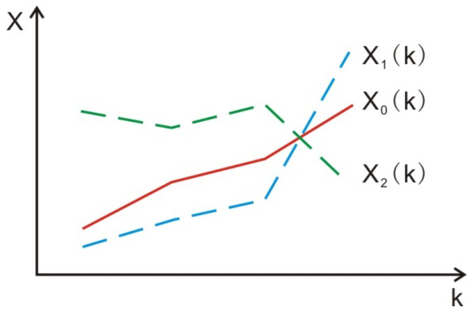
GRA is a calculation of the geometric proximity between different discrete sequences, a reference sequence, and at least one comparison sequence within a system. The proximity is described by the grey relational grade, which is a measure of the similarities of discrete data that can be arranged in sequential order. Further information on this concept and examples of its application are available in the literature [23].

The basic concept of the technique is illustrated with sample time series in Figure 4. The function X₀(k) denotes the reference series, and X₁(k) and X₂(k) denote the comparison series. The similarity between X₀(k) and X₁(k) is “greater” than that between X₀(k) and X₂(k). Thus, the relational grade between X₀(k) and X₁(k) can be regarded as higher and that between X₀(k) and X₂(k) as lower. This geometric consideration is effectively an analysis of the geometric proximity between different discrete series.

Figure 4. Similarity and difference of sequences.

Figure 4. Similarity and difference of sequences.

3.2.2. Basic Approach

The GRA method involves the following steps:

(1) Determining the reference and comparison series

The time series X₀’ is referred to as the reference series, which represents the characteristics of the system. The m time series X_i’ is a comparison series of factors influencing the characteristics of the system.

(1)

(2)

Here, k and i represent the period and evaluating factors, respectively.

(2) Data pre-processing

Pre-processing is typically required, because the range and units of one data sequence often differ from those of others. This processing is a way of transferring the original X₀’, X_i’ to comparable sequences X₀, X_i. Various methods have been proposed for processing of data for grey relational analysis [25], the most basic forms are listed below:

(3)

(4)

(5)

where, X_i’ denotes the original sequences; and X_i the sequences after data processing; X_i’ is the average value of sequence X_i’.

(3) Determining the deviation sequences Δ_0i

We determine the deviation sequences Δ_0i between the corresponding values in the reference and comparison series, and the maximum and minimum values, which are denoted by maxΔ_0i(k) and minΔ_0i(k), respectively.

Δ_0i(k) = |x₀(k) − x_i(k)|

(6)

(4) Calculation of the grey relational coefficient ξ_i(k) of each series

(7)

Here, ρ ∈(0, 1] is the distinguishing coefficient, which differentiates the degree of proximity of X₀ and X_i, such that ξ_i(k)∈[0,1]. This value can be adjusted based on the actual system requirements. Generally, ρ is taken as 0.5 based on the minimum information [37].

(5) Calculation of the grey relational grade γ_i

(8)

4. Results and Discussion

4.1. Groundwater Flow Dynamics

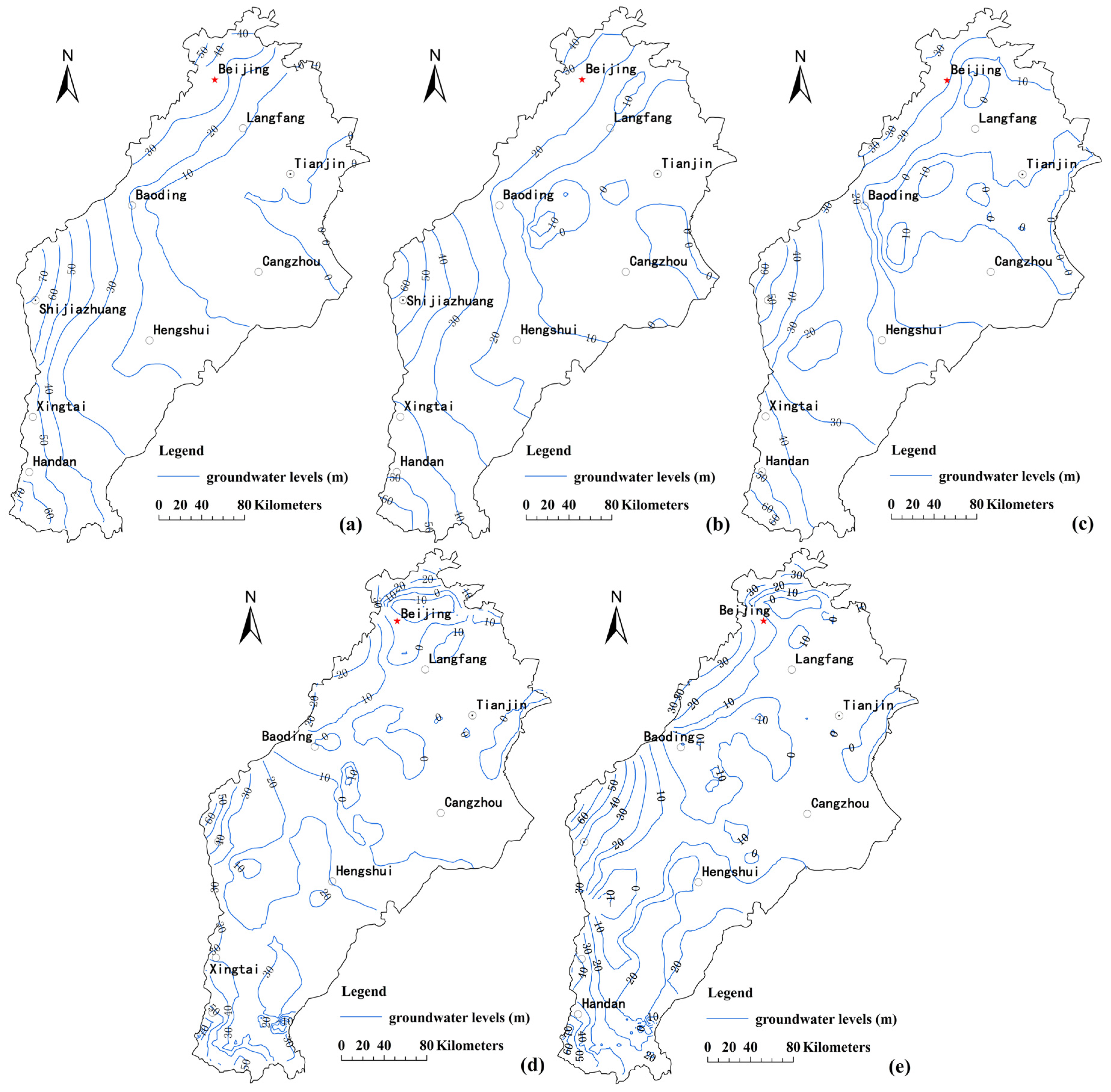
The simulated results were used to illustrate the groundwater change in the study area during the 50-year period. We selected the shallow groundwater levels in 1965, 1975, 1985, 1995, and 2005 as representative of their respective decades; these are presented in Figure 5.

In 1965, groundwater flow extended from the mountains to Bohai Bay, with groundwater levels of 70 m near Shijiazhuang (at the mountain) and 0 m near Tianjin (coastal area). The average water table depth was 10 m. Conversely, in 1975, cones of depression were observed in parts of Beijing and Baoding. The natural flow fields changed as the groundwater began to flow into the center of the cones. The groundwater level decreased to approximately 60 m near Shijiazhuang, whereas groundwater levels of 30 m expanded to the west, with an average water table depth of 11 m.

Overall groundwater levels had declined and additional cones of depression had formed by 1985. Regions with groundwater levels below 30 m continued expanding to the west, with an average water table depth of 16 m.

Further decline in groundwater levels was observed by 1995. In addition to the enhanced cones of depression in Beijing, Ning-Bo-Longin, and Xingtai, new cones formed in other locations (e.g., Handan). The groundwater levels below 30 m continued to expand westward, reaching the mountain front, with an average water table depth of 24 m.

By 2005, the overall decline of groundwater levels had stopped, and groundwater levels rose in the cone at Beijing. However, the cones of depression at Baoding, Lixian, and Bazhou merged, and the cone at Ning-Bo-Long expanded into the central plain. These results are in agreement with field investigations [16]. The region with groundwater levels below 30 m continued to shift westward, and the average water table depth was 22 m.

Figure 5. Simulated groundwater levels: (a) 1965; (b) 1975; (c) 1985; (d) 1995; (e) 2005.

Figure 5. Simulated groundwater levels: (a) 1965; (b) 1975; (c) 1985; (d) 1995; (e) 2005.

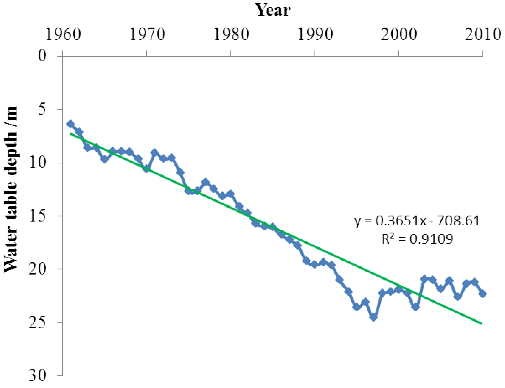
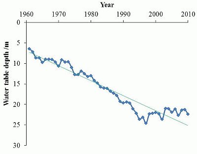
Based on these results, we conclude that the simulated groundwater table depths increased at an average rate of 0.36 m/a over the 50-year period studied (Figure 6). Similar results were obtained in the work of Cao [38], in which a rate of 0.3 m/a was determined for the NCP.

Figure 6. Change of annual average water table depth during 1961–2010.

Figure 6. Change of annual average water table depth during 1961–2010.

4.2. Factors Influencing Groundwater Levels

The flow fields in the study area have changed dramatically because of changes in climate and human activities: the former affects groundwater primarily via precipitation and evaporation, whereas the latter affect groundwater largely through exploitation and the construction of reservoirs.

4.2.1. Climate Change

In arid (and semi-arid) landscapes, climate change has a great impact on water resources. In particular, groundwater dynamics are affected by precipitation infiltration and phreatic evaporation, which result from changes in precipitation and temperature that affect evaporation indirectly. Over the past 50–100 years, the climate of the NCP has undergone obvious changes, with an increasing trend in temperature and decreasing trend in precipitation [39]. We measured these long-term trends in mean annual precipitation and temperature in the study area using a nonparametric technique (the Mann–Kendall test [40,41,42]).

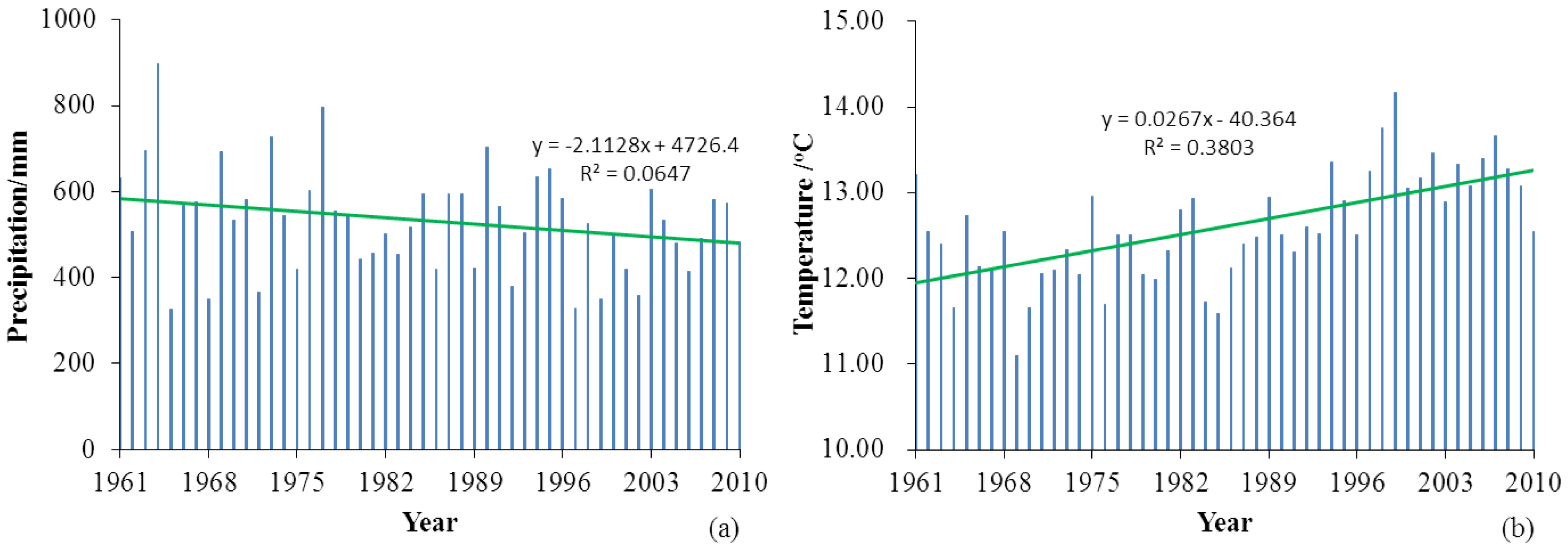
Based on the precipitation data series from the China Meteorological Data Sharing Service system, annual average precipitation in the study area was 531.39 mm in 1961–2010. We observed a clear inter-annual variation in precipitation, and what appears to be a 12-year trend (Figure 7a). Ip [43] found an inter-annual 4–7 year component and inter-decadal 19-year periodicity in North China, whereas Kuang [44] calculated periodicities of 6–7, 21–22, and 35–36 years. These different results could be caused by the length of the time series applied. The long-term trend for the precipitation series showed that the nonparametric Mann–Kendall test supported H₀ at the 5% significance level (Table 1), which means that precipitation had a decreasing trend that was not significant.

Figure 7. (a) Annual average precipitation and (b) annual average temperature in the study area in 1961–2010.

Figure 7. (a) Annual average precipitation and (b) annual average temperature in the study area in 1961–2010.

Table 1. Monotonic trend tests for the precipitation and temperature time series.

Item	Mann–Kendall test
	Z0	β	H0
Precipitation	−1.58	−1.78	S
Temperature	4.48	0.028	C

Notes: C Contradict; S Support; Significance level p=5%; Z₀ is statistics of Mann–Kendall test.

Table 1. Monotonic trend tests for the precipitation and temperature time series.

Item	Mann–Kendall test
	Z0	β	H0
Precipitation	−1.58	−1.78	S
Temperature	4.48	0.028	C

Notes: C Contradict; S Support; Significance level p=5%; Z₀ is statistics of Mann–Kendall test.

Based on the temperature data series from the China Meteorological Data Sharing Service system, annual average temperature in the study area was 12.6 °C in 1961–2010 (Figure 7b). The Mann–Kendall test for temperature change contradicts hypothesis H₀ (Table 1); that is, an increasing trend for the temperature series was found to be significant at the 5% level. Temperature increased at a rate of 0.28 °C/10 a, similar to results in previous studies [39,45]. This increasing trend in mean annual temperature resulted in an increase in water vapor capacity. Increased evaporation caused by the rise in temperature would have exacerbated the loss of groundwater through evaporation in the study area during the past five decades. Groundwater table depths declined over the study period, suggesting that climate change may have accelerated the decrease in groundwater levels.

4.2.2. Human Activities

Groundwater exploitation increases the discharge of groundwater, changing the natural flow field, and has become the most important discharge route for groundwater. Construction of reservoirs in the upstream areas has reduced groundwater recharge by surface water in the plain.

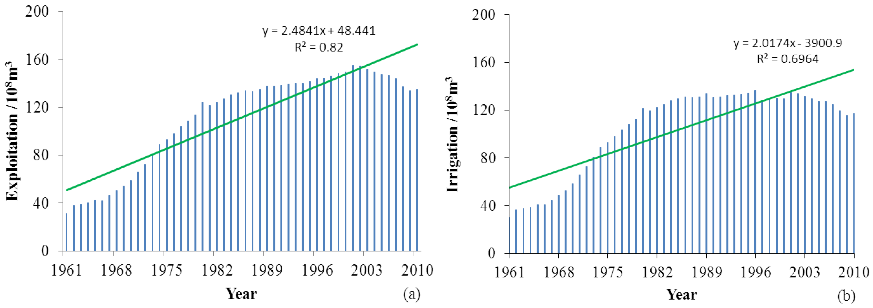
We obtained groundwater exploitation data from the Hydrological Bureau of each municipality and from previous field research [19,35,36,46,47,48]. During the study period, groundwater abstraction has progressed from a random and disorderly activity to a systematic process. Increasing volumes of water have been pumped from greater depths [29], especially since the 1970s (Figure 8a). In the study area, the total recharge was 14.4 billion m³/a from 1991 to 2003, whereas the total discharge was 16.6 billion m³/a; that is, groundwater was over-exploited with a net abstraction of 2.2 billion m³/a [19]. The annual average abstraction in the study area was estimated at 11.2 billion m³/a from 1961 to 2010 with agriculture accounting for an estimated 73%–84% of the total exploitation [49].

Figure 8. (a) Groundwater exploitation and (b) irrigation in the study area during 1961–2010.

Figure 8. (a) Groundwater exploitation and (b) irrigation in the study area during 1961–2010.

River leakage in the plains is one of the primary recharge sources for groundwater, and old channels with good permeability allow the passage of surface water to the groundwater system. However, many water projects built since the 1960s in the upstream regions of rivers retain runoff, reducing groundwater recharge by surface water in the plains. According to Zhang et al. [19], the total water released from the reservoirs was 53.0 billion m³/a from 1960 to 2002, 2.2 billion m³/a in the 1960s, and only 0.63 billion in the 1980s. The reasons for this are twofold: upstream water use increased with the development of society and economy; combined with changes in climate including decreasing precipitation (i.e., decreasing runoff) and increasing temperature. Groundwater levels were reduced further when the decreased runoff resulted in less groundwater recharge.

Irrigation return flow, following exploitation for agriculture and water release from reservoirs, has become a new source of groundwater recharge. Groundwater is the primacy source for irrigation, accounting for 81%–93% of total irrigation water in the NCP [50]. The total amount of groundwater used for irrigation in the study area was estimated based on the volume of groundwater abstracted for agriculture and the ratio above, giving an estimate of 10.5 billion m³/a from 1961 to 2010. The estimated volume exhibited a trend similar to that of groundwater exploitation (Figure 8b).

4.3. GRA between Water Table Depth and Influencing Factors

Declining groundwater levels pose many environmental and geological problems. Therefore, it is important to understand which of the several factors affecting groundwater levels are the true driving forces. Based on the simulated groundwater levels and the factors described above, we used GRA to rank the influence of the factors.

(1) Calculation of the reference and comparison series

X₀’ is the reference series, representing water table depth, and X_i’ is the comparison series, considered to be factors that influence water table depth. The study period was 50 years, and the series were as follows:

X₀′ = {x₀′(1),x₀′(2),…x₀′(50)} -----Water table depth

(9)

X₁′ = {x₁′(1),x₁′(2),…x₁′(50)} -----Precipitation infiltration

(10)

X₂′ = {x₂′(1),x₂′(2),…x₂′(50)} -----Phreatic evaporation

(11)

X₃′ = {x₃′(1),x₃′(2),…x₃′(50)} -----Groundwater exploitation

(12)

X₄′ = {x₄′(1),x₄′(2),…x₄′(50)} -----River leakage

(13)

X₅′ = {x₅′(1),x₅′(2),…x₅′(50)} -----Irrigation return flow

(14)

(2) Data pre-processing

The results of the sequences are presented in Table 2.

Table 2. The sequences after data pre-processing.

n	X0	X1	X2	X3	X4	X5
1	0.397	0.863	1.515	0.277	1.886	0.551
2	0.444	0.690	1.511	0.337	1.886	0.670
3	0.533	0.947	1.386	0.347	1.886	0.689
4	0.532	1.224	1.039	0.357	1.886	0.709
5	0.601	0.447	1.483	0.378	1.886	0.753
6	0.556	0.776	1.261	0.377	1.886	0.750
7	0.555	0.787	1.248	0.413	1.886	0.822
8	0.559	0.478	1.513	0.450	1.886	0.895
9	0.597	0.944	1.203	0.487	1.886	0.969
10	0.658	0.727	1.227	0.524	1.886	1.076
11	0.564	0.963	1.623	0.588	1.252	0.643
12	0.599	0.609	1.873	0.647	1.252	0.711
13	0.593	1.207	1.519	0.720	1.252	0.791
14	0.679	0.903	1.601	0.796	1.252	0.871
15	0.783	0.695	1.572	0.832	1.252	0.909
16	0.784	0.998	1.449	0.874	1.252	0.961
17	0.734	1.322	1.475	0.929	1.252	1.015
18	0.772	0.919	1.525	0.970	1.252	1.061
19	0.815	0.905	1.385	1.018	1.252	1.101
20	0.802	0.735	1.408	1.109	1.252	1.191
21	0.876	0.851	0.843	1.088	0.514	0.913
22	0.913	0.938	0.840	1.112	0.514	0.933
23	0.971	0.849	0.790	1.138	0.514	0.955
24	0.988	0.966	0.761	1.168	0.514	0.980
25	0.995	1.109	0.649	1.184	0.514	0.993
26	1.038	0.782	0.805	1.196	0.514	1.005
27	1.065	1.108	0.707	1.193	0.514	0.999
28	1.099	1.108	0.752	1.208	0.514	1.005
29	1.189	0.787	0.811	1.234	0.514	1.026
30	1.210	1.313	0.654	1.232	0.514	1.001
31	1.197	1.293	0.629	1.235	0.737	1.143
32	1.215	0.868	0.707	1.249	0.737	1.155
33	1.302	1.154	0.705	1.251	0.737	1.158
34	1.367	1.448	0.705	1.253	0.737	1.161
35	1.459	1.493	0.690	1.265	0.737	1.171
36	1.427	1.335	0.671	1.287	0.737	1.191
37	1.519	0.752	0.740	1.294	0.737	1.119
38	1.379	1.201	0.635	1.308	0.737	1.127
39	1.370	0.801	0.705	1.329	0.737	1.136
40	1.355	1.146	0.701	1.336	0.737	1.130
41	1.377	0.980	0.833	1.388	0.737	1.234
42	1.459	0.840	0.834	1.382	0.596	1.228
43	1.298	1.418	0.688	1.356	0.596	1.205
44	1.299	1.247	0.726	1.335	0.596	1.187
45	1.353	1.125	0.729	1.315	0.596	1.169
46	1.307	0.967	0.641	1.314	0.596	1.168
47	1.399	1.149	0.656	1.287	0.596	1.144
48	1.320	1.361	0.525	1.228	0.596	1.092
49	1.313	1.343	0.523	1.195	0.596	1.063
50	1.383	1.132	0.525	1.209	0.596	1.074

Table 2. The sequences after data pre-processing.

n	X0	X1	X2	X3	X4	X5
1	0.397	0.863	1.515	0.277	1.886	0.551
2	0.444	0.690	1.511	0.337	1.886	0.670
3	0.533	0.947	1.386	0.347	1.886	0.689
4	0.532	1.224	1.039	0.357	1.886	0.709
5	0.601	0.447	1.483	0.378	1.886	0.753
6	0.556	0.776	1.261	0.377	1.886	0.750
7	0.555	0.787	1.248	0.413	1.886	0.822
8	0.559	0.478	1.513	0.450	1.886	0.895
9	0.597	0.944	1.203	0.487	1.886	0.969
10	0.658	0.727	1.227	0.524	1.886	1.076
11	0.564	0.963	1.623	0.588	1.252	0.643
12	0.599	0.609	1.873	0.647	1.252	0.711
13	0.593	1.207	1.519	0.720	1.252	0.791
14	0.679	0.903	1.601	0.796	1.252	0.871
15	0.783	0.695	1.572	0.832	1.252	0.909
16	0.784	0.998	1.449	0.874	1.252	0.961
17	0.734	1.322	1.475	0.929	1.252	1.015
18	0.772	0.919	1.525	0.970	1.252	1.061
19	0.815	0.905	1.385	1.018	1.252	1.101
20	0.802	0.735	1.408	1.109	1.252	1.191
21	0.876	0.851	0.843	1.088	0.514	0.913
22	0.913	0.938	0.840	1.112	0.514	0.933
23	0.971	0.849	0.790	1.138	0.514	0.955
24	0.988	0.966	0.761	1.168	0.514	0.980
25	0.995	1.109	0.649	1.184	0.514	0.993
26	1.038	0.782	0.805	1.196	0.514	1.005
27	1.065	1.108	0.707	1.193	0.514	0.999
28	1.099	1.108	0.752	1.208	0.514	1.005
29	1.189	0.787	0.811	1.234	0.514	1.026
30	1.210	1.313	0.654	1.232	0.514	1.001
31	1.197	1.293	0.629	1.235	0.737	1.143
32	1.215	0.868	0.707	1.249	0.737	1.155
33	1.302	1.154	0.705	1.251	0.737	1.158
34	1.367	1.448	0.705	1.253	0.737	1.161
35	1.459	1.493	0.690	1.265	0.737	1.171
36	1.427	1.335	0.671	1.287	0.737	1.191
37	1.519	0.752	0.740	1.294	0.737	1.119
38	1.379	1.201	0.635	1.308	0.737	1.127
39	1.370	0.801	0.705	1.329	0.737	1.136
40	1.355	1.146	0.701	1.336	0.737	1.130
41	1.377	0.980	0.833	1.388	0.737	1.234
42	1.459	0.840	0.834	1.382	0.596	1.228
43	1.298	1.418	0.688	1.356	0.596	1.205
44	1.299	1.247	0.726	1.335	0.596	1.187
45	1.353	1.125	0.729	1.315	0.596	1.169
46	1.307	0.967	0.641	1.314	0.596	1.168
47	1.399	1.149	0.656	1.287	0.596	1.144
48	1.320	1.361	0.525	1.228	0.596	1.092
49	1.313	1.343	0.523	1.195	0.596	1.063
50	1.383	1.132	0.525	1.209	0.596	1.074

(3) Calculation of the deviation sequences Δ_0i

The deviation sequences were calculated using Equation 6: Δ₀₁(1) = |x₀(1)−x₁(1)| = |0.397–0.863| = 0.466, Δ₀₁(2) = |x₀(2)−x₁(2)| = |0.397–1.515| = 1.118. The same method was adopted for i = 1–5 and the results for all Δ_0i are presented in Table 3. Based on these results, maxΔ_0i(k) = 1.442 and minΔ_0i(k) = 0.002.

Table 3. The deviation sequences.

n	Δ01	Δ02	Δ03	Δ04	Δ05
1	0.466	1.118	0.120	1.489	0.154
2	0.246	1.068	0.107	1.442	0.226
3	0.415	0.854	0.186	1.354	0.157
4	0.692	0.507	0.175	1.354	0.177
5	0.154	0.883	0.222	1.286	0.152
6	0.220	0.705	0.179	1.330	0.194
7	0.231	0.692	0.142	1.331	0.267
8	0.081	0.954	0.109	1.327	0.336
9	0.347	0.607	0.110	1.289	0.372
10	0.069	0.569	0.134	1.228	0.418
11	0.399	1.059	0.024	0.688	0.079
12	0.009	1.274	0.048	0.652	0.112
13	0.614	0.926	0.127	0.659	0.198
14	0.224	0.922	0.117	0.573	0.192
15	0.088	0.789	0.048	0.469	0.126
16	0.214	0.665	0.090	0.468	0.177
17	0.588	0.741	0.194	0.517	0.281
18	0.148	0.753	0.199	0.480	0.290
19	0.091	0.571	0.203	0.437	0.287
20	0.068	0.606	0.307	0.449	0.389
21	0.026	0.033	0.212	0.362	0.037
22	0.025	0.074	0.199	0.399	0.020
23	0.122	0.181	0.167	0.456	0.016
24	0.022	0.227	0.180	0.473	0.008
25	0.114	0.346	0.188	0.481	0.002
26	0.257	0.233	0.158	0.524	0.034
27	0.044	0.358	0.128	0.550	0.066
28	0.008	0.347	0.109	0.585	0.094
29	0.403	0.379	0.044	0.675	0.164
30	0.103	0.556	0.022	0.696	0.209
31	0.096	0.567	0.039	0.459	0.054
32	0.347	0.508	0.034	0.477	0.060
33	0.148	0.597	0.050	0.564	0.144
34	0.080	0.662	0.114	0.630	0.206
35	0.034	0.769	0.194	0.722	0.288
36	0.092	0.756	0.140	0.690	0.236
37	0.767	0.779	0.225	0.782	0.400
38	0.178	0.744	0.071	0.642	0.252
39	0.570	0.665	0.041	0.633	0.234
40	0.209	0.654	0.019	0.617	0.224
41	0.397	0.544	0.011	0.640	0.143
42	0.619	0.625	0.077	0.863	0.231
43	0.120	0.610	0.058	0.702	0.093
44	0.052	0.573	0.036	0.703	0.112
45	0.228	0.624	0.038	0.757	0.184
46	0.340	0.666	0.008	0.710	0.139
47	0.250	0.743	0.112	0.803	0.256
48	0.041	0.795	0.092	0.724	0.228
49	0.030	0.790	0.118	0.717	0.251
50	0.251	0.858	0.175	0.787	0.309

Table 3. The deviation sequences.

n	Δ01	Δ02	Δ03	Δ04	Δ05
1	0.466	1.118	0.120	1.489	0.154
2	0.246	1.068	0.107	1.442	0.226
3	0.415	0.854	0.186	1.354	0.157
4	0.692	0.507	0.175	1.354	0.177
5	0.154	0.883	0.222	1.286	0.152
6	0.220	0.705	0.179	1.330	0.194
7	0.231	0.692	0.142	1.331	0.267
8	0.081	0.954	0.109	1.327	0.336
9	0.347	0.607	0.110	1.289	0.372
10	0.069	0.569	0.134	1.228	0.418
11	0.399	1.059	0.024	0.688	0.079
12	0.009	1.274	0.048	0.652	0.112
13	0.614	0.926	0.127	0.659	0.198
14	0.224	0.922	0.117	0.573	0.192
15	0.088	0.789	0.048	0.469	0.126
16	0.214	0.665	0.090	0.468	0.177
17	0.588	0.741	0.194	0.517	0.281
18	0.148	0.753	0.199	0.480	0.290
19	0.091	0.571	0.203	0.437	0.287
20	0.068	0.606	0.307	0.449	0.389
21	0.026	0.033	0.212	0.362	0.037
22	0.025	0.074	0.199	0.399	0.020
23	0.122	0.181	0.167	0.456	0.016
24	0.022	0.227	0.180	0.473	0.008
25	0.114	0.346	0.188	0.481	0.002
26	0.257	0.233	0.158	0.524	0.034
27	0.044	0.358	0.128	0.550	0.066
28	0.008	0.347	0.109	0.585	0.094
29	0.403	0.379	0.044	0.675	0.164
30	0.103	0.556	0.022	0.696	0.209
31	0.096	0.567	0.039	0.459	0.054
32	0.347	0.508	0.034	0.477	0.060
33	0.148	0.597	0.050	0.564	0.144
34	0.080	0.662	0.114	0.630	0.206
35	0.034	0.769	0.194	0.722	0.288
36	0.092	0.756	0.140	0.690	0.236
37	0.767	0.779	0.225	0.782	0.400
38	0.178	0.744	0.071	0.642	0.252
39	0.570	0.665	0.041	0.633	0.234
40	0.209	0.654	0.019	0.617	0.224
41	0.397	0.544	0.011	0.640	0.143
42	0.619	0.625	0.077	0.863	0.231
43	0.120	0.610	0.058	0.702	0.093
44	0.052	0.573	0.036	0.703	0.112
45	0.228	0.624	0.038	0.757	0.184
46	0.340	0.666	0.008	0.710	0.139
47	0.250	0.743	0.112	0.803	0.256
48	0.041	0.795	0.092	0.724	0.228
49	0.030	0.790	0.118	0.717	0.251
50	0.251	0.858	0.175	0.787	0.309

(4) Calculation of the grey relational coefficient ξ_i(k)

The parameters were calculated using Equation 7 and the results are presented in Table 4.

(5) Calculation of the grey relational grade γ_i of each series

The parameters were calculated using Equation 8, and the results are presented in Table 4.

Table 4. The calculated grey relational coefficient and grey relational grade for five comparison sequences

n	ξ1	ξ2	ξ3	ξ4	ξ5
1	0.609	0.393	0.860	0.327	0.827
2	0.748	0.405	0.874	0.334	0.764
3	0.637	0.460	0.798	0.349	0.824
4	0.512	0.589	0.807	0.349	0.806
5	0.827	0.451	0.767	0.361	0.829
6	0.769	0.508	0.803	0.353	0.791
7	0.760	0.512	0.838	0.353	0.732
8	0.902	0.432	0.872	0.353	0.685
9	0.677	0.545	0.871	0.360	0.662
10	0.915	0.561	0.846	0.371	0.635
11	0.646	0.406	0.972	0.514	0.905
12	0.990	0.363	0.941	0.527	0.868
13	0.542	0.439	0.853	0.524	0.788
14	0.765	0.440	0.863	0.559	0.792
15	0.894	0.479	0.940	0.608	0.854
16	0.774	0.522	0.892	0.609	0.805
17	0.553	0.495	0.791	0.584	0.722
18	0.833	0.491	0.787	0.602	0.716
19	0.891	0.560	0.783	0.625	0.718
20	0.917	0.545	0.704	0.618	0.652
21	0.969	0.959	0.776	0.668	0.955
22	0.970	0.910	0.786	0.646	0.977
23	0.858	0.802	0.814	0.614	0.982
24	0.974	0.764	0.803	0.606	0.993
25	0.867	0.678	0.796	0.602	1.000
26	0.740	0.758	0.823	0.581	0.959
27	0.946	0.671	0.852	0.569	0.919
28	0.992	0.677	0.872	0.554	0.888
29	0.644	0.658	0.945	0.518	0.818
30	0.878	0.567	0.974	0.511	0.778
31	0.885	0.562	0.952	0.613	0.934
32	0.677	0.589	0.958	0.604	0.926
33	0.833	0.549	0.938	0.563	0.836
34	0.903	0.523	0.867	0.536	0.781
35	0.958	0.486	0.791	0.501	0.717
36	0.890	0.490	0.840	0.513	0.756
37	0.486	0.482	0.765	0.482	0.645
38	0.805	0.494	0.914	0.531	0.743
39	0.561	0.522	0.949	0.534	0.757
40	0.778	0.526	0.978	0.541	0.765
41	0.647	0.572	0.988	0.532	0.837
42	0.540	0.538	0.906	0.457	0.760
43	0.861	0.544	0.929	0.509	0.888
44	0.935	0.559	0.955	0.508	0.868
45	0.762	0.538	0.953	0.490	0.800
46	0.682	0.522	0.993	0.505	0.841
47	0.745	0.494	0.868	0.475	0.741
48	0.949	0.477	0.890	0.501	0.762
49	0.964	0.479	0.862	0.503	0.744
50	0.744	0.458	0.808	0.480	0.702
γi	0.792	0.549	0.868	0.511	0.809
Grey relational order	3	4	1	5	2

Table 4. The calculated grey relational coefficient and grey relational grade for five comparison sequences

n	ξ1	ξ2	ξ3	ξ4	ξ5
1	0.609	0.393	0.860	0.327	0.827
2	0.748	0.405	0.874	0.334	0.764
3	0.637	0.460	0.798	0.349	0.824
4	0.512	0.589	0.807	0.349	0.806
5	0.827	0.451	0.767	0.361	0.829
6	0.769	0.508	0.803	0.353	0.791
7	0.760	0.512	0.838	0.353	0.732
8	0.902	0.432	0.872	0.353	0.685
9	0.677	0.545	0.871	0.360	0.662
10	0.915	0.561	0.846	0.371	0.635
11	0.646	0.406	0.972	0.514	0.905
12	0.990	0.363	0.941	0.527	0.868
13	0.542	0.439	0.853	0.524	0.788
14	0.765	0.440	0.863	0.559	0.792
15	0.894	0.479	0.940	0.608	0.854
16	0.774	0.522	0.892	0.609	0.805
17	0.553	0.495	0.791	0.584	0.722
18	0.833	0.491	0.787	0.602	0.716
19	0.891	0.560	0.783	0.625	0.718
20	0.917	0.545	0.704	0.618	0.652
21	0.969	0.959	0.776	0.668	0.955
22	0.970	0.910	0.786	0.646	0.977
23	0.858	0.802	0.814	0.614	0.982
24	0.974	0.764	0.803	0.606	0.993
25	0.867	0.678	0.796	0.602	1.000
26	0.740	0.758	0.823	0.581	0.959
27	0.946	0.671	0.852	0.569	0.919
28	0.992	0.677	0.872	0.554	0.888
29	0.644	0.658	0.945	0.518	0.818
30	0.878	0.567	0.974	0.511	0.778
31	0.885	0.562	0.952	0.613	0.934
32	0.677	0.589	0.958	0.604	0.926
33	0.833	0.549	0.938	0.563	0.836
34	0.903	0.523	0.867	0.536	0.781
35	0.958	0.486	0.791	0.501	0.717
36	0.890	0.490	0.840	0.513	0.756
37	0.486	0.482	0.765	0.482	0.645
38	0.805	0.494	0.914	0.531	0.743
39	0.561	0.522	0.949	0.534	0.757
40	0.778	0.526	0.978	0.541	0.765
41	0.647	0.572	0.988	0.532	0.837
42	0.540	0.538	0.906	0.457	0.760
43	0.861	0.544	0.929	0.509	0.888
44	0.935	0.559	0.955	0.508	0.868
45	0.762	0.538	0.953	0.490	0.800
46	0.682	0.522	0.993	0.505	0.841
47	0.745	0.494	0.868	0.475	0.741
48	0.949	0.477	0.890	0.501	0.762
49	0.964	0.479	0.862	0.503	0.744
50	0.744	0.458	0.808	0.480	0.702
γi	0.792	0.549	0.868	0.511	0.809
Grey relational order	3	4	1	5	2

The factors that control water table depth, in order of decreasing importance, are X₃ (groundwater exploitation), X₅ (irrigation return flow), X₁ (precipitation infiltration), X₂ (phreatic evaporation), and X₄ (river leakage) (i.e., γ₃ > γ₅ > γ₁ > γ₂ > γ₄). Exploitation and irrigation return flow represent human influence, whereas precipitation infiltration represents climate change. Therefore, human activities are the major factors responsible for declining groundwater levels in the study area. The correlation between river leakage and water table depth was the weakest of all factors studied, which could be caused by the small contribution of river leakage to groundwater recharge since the 1980s.

It was noted that data pre-processing caused some fluctuations of the grey relational grade. We therefore used two additional methods Equations (4) and (5) for data pre-processing to obtain grey relational grades. The three methods obtained the same grey relational order, indicating that the results are robust.

The GRA results, suggesting human activities (particularly exploitation) are the primary driving forces of groundwater change, are consistent with previous estimates using the projection pursuit regression (PPR) technique [51]. These analyses of historical groundwater level changes since 1960 have generally shown that groundwater is in a state of imbalance. The large cones of depression that have formed in the study area (likely caused by human activities) are representative of unsustainable groundwater exploitation.

The principle of sustainability, defined by the United Nations Commission on Sustainable Development in 1987, calls for satisfying current needs without compromising the needs of future generations, and has been adopted for the management of groundwater resources development. Sophocleous [52] noted that the sustainable yield of an aquifer must be considerably less than recharge if adequate amounts of water are to be available to sustain both the quantity and quality of streams, springs, wetlands, and groundwater-dependent ecosystems. In this context, sustainable exploitation involves compromise to ensure that resources can be maintained for an infinite time without causing serious environmental, economic, or social consequences. To maintain groundwater equilibrium, groundwater abstraction should not exceed the recharge rate minus other conditions.

Many previous studies have investigated ways to achieve groundwater sustainability, including liming groundwater abstraction, increasing groundwater recharge, conjunctive use of surface and groundwater, and better use of groundwater storage [53,54]. Several effective approaches have been attempted in the NCP [55]. The South-to-North Water Diversion Project (SNWDP) is proposed as a significant method to manage and prevent the continued shortage of groundwater resources in northern China. This route conveys water from Danjiangkou, which is located in a branch of Yangzi River, to Beijing and Tianjin in the north via a 1241.2 km long main canal [56]. The first phase of the project will be completed after the flood season in 2014, supplying the NCP with 5.7 billion m³/a of water [57]. This approach should remediate the groundwater cone to some extent; however, considerable time will be required to recover the groundwater environment [58].

5. Conclusions

We used a groundwater flow model to determine groundwater change in the NCP. Over the past 50 years, groundwater conditions have changed dramatically, with declining levels and the development of cones of depression. The primary factors influencing groundwater levels are precipitation, temperature, groundwater exploitation, and the construction of reservoirs. Both climate change and human activities contribute to the changes, although groundwater exploitation was found to be the major driving factor.

GRA was able to separate the influence of different factors associated with groundwater dynamics, calculate the grey relational order, and produce reasonable results. It is therefore suitable and sensitive enough to identify major and minor driving forces.

Many different sustainable development strategies will be required to stop the decline in groundwater levels. At present, the implementation of the SNWDP will significantly reduce water shortages and the deterioration of the groundwater ecological environment in the NCP. The project will also provide valuable information for groundwater sustainable development strategies in other hotspots facing water shortages.

Although the concept underpinning groundwater sustainability is clear, the criteria for developing current sustainability projects cannot yet be evaluated, because both climate and socio-economic patterns are changing. We describe a method that offers promise in identifying those criteria. In particular, the combination of numerical simulation and grey system theory will be useful in developing criteria to achieve sustainable development. The results presented here may be applicable for similar areas of water scarcity.

The scope of this study was restricted by the limited data available on climate change and human activities. We were not able to completely separate their respective influences on groundwater. Therefore, further study of the impact of human activities on climate change in the context of groundwater will be important in future.

References

1. Kemper, K. Groundwater—From development to management. Hydrogeol. J. 2004, 12, 3–5. [Google Scholar] [CrossRef]
2. De Vries, J.; Simmers, I. Groundwater recharge: An overview of processes and challenges. Hydrogeol. J. 2002, 10, 5–17. [Google Scholar] [CrossRef]
3. Chen, H.; Wang, S.; Gao, Z.; Hu, Y. Artificial Neural Network Approach for Quantifying Climate Change and Human Activities Impacts on Shallow Groundwater Level—A Case Study of Wuqiao in North China Plain; IEEE: New York, NY, USA, 2010. [Google Scholar]
4. Hsu, K.-C.; Yeh, H.-F.; Chen, Y.-C.; Lee, C.-H.; Wang, C.-H.; Chiu, F.-S. Basin-scale groundwater response to precipitation variation and anthropogenic pumping in Chih-ben watershed, Taiwan. Hydrogeol. J. 2012, 20, 499–517. [Google Scholar] [CrossRef]
5. Hao, X.; Chen, Y.; Xu, C.; Li, W. Impacts of climate change and human activities on the surface runoff in the Tarim river basin over the last fifty years. Water Resour. Manag. 2008, 22, 1159–1171. [Google Scholar] [CrossRef]
6. Bloomfield, J.P.; Gaus, I.; Wade, S.D. A method for investigating the potential impacts of climate-change scenarios on annual minimum groundwater levels. Water Environ. J. 2003, 17, 86–91. [Google Scholar] [CrossRef] [Green Version]
7. Scibek, J.; Allen, D.M. Modeled impacts of predicted climate change on recharge and groundwater levels. Water Resour. Res. 2006, 42, W11405. [Google Scholar]
8. Waibel, M.S.; Gannett, M.W.; Chang, H.; Hulbe, C.L. Spatial variability of the response to climate change in regional groundwater systems—Examples from simulations in the deschutes basin, oregon. J. Hydrol. 2013, 486, 187–201. [Google Scholar] [CrossRef]
9. Konikow, L.; Kendy, E. Groundwater depletion: A global problem. Hydrogeol. J. 2005, 13, 317–320. [Google Scholar] [CrossRef]
10. Shah, T.; Molden, D.; Sakthivadivel, R.; Seckler, D. Global groundwater situation: Opportunities and challenges. Eco. Polit. Wkly. 2001, 36, 4142–4150. [Google Scholar]
11. Wada, Y.; van Beek, L.P.H.; van Kempen, C.M.; Reckman, J.W.T.M.; Vasak, S.; Bierkens, M.F.P. Global depletion of groundwater resources. Geophys. Res. Lett. 2010, 37, L20402. [Google Scholar]
12. Manca, F.; Capelli, G.; La Vigna, F.; Mazza, R.; Pascarella, A. Wind-induced salt-wedge intrusion in the Tiber river mouth (Rome–Central Italy). Environ. Earth Sci. 2014. [Google Scholar] [CrossRef]
13. Custodio, E. Aquifer overexploitation: What does it mean? Hydrogeol. J. 2002, 10, 254–277. [Google Scholar] [CrossRef]
14. Zheng, C.; Liu, J.; Cao, G.; Kendy, E.; Wang, H.; Jia, Y. Can China cope with its water crisis?—Perspectives from the North China Plain. Ground Water 2010, 48, 350–354. [Google Scholar] [CrossRef]
15. Liu, C.; Yu, J.; Kendy, E. Groundwater exploitation and its impact on the environment in the North China Plain. Water Int. 2001, 26, 265–272. [Google Scholar] [CrossRef]
16. Fei, Y.; Zhang, Z.; Zhang, F.E.; Wang, Z.; Chen, Z.; Chen, J.; Qian, Y.; Li, Y. An analysis of the influence of human activity and climate change on water resources of the North China Plain. Acta Geosci. Sin. 2007, 28, 567–571. (In Chinese) [Google Scholar]
17. Fei, Y.; Miao, J.; Zhang, Z.; Chen, Z.; Song, H.; Yang, M. Analysis on evolution of groundwater depression cones and its leading factors in North China Plain. Resour. Sci. 2009, 31, 394–399. (In Chinese) [Google Scholar]
18. Zhu, L.; Gong, H.; Li, X.; Li, Y.; Su, X.; Guo, G. Comprehensive analysis and artificial intelligent simulation of land subsidence of Beijing, China. Chin. Geogr. Sci. 2013, 23, 237–248. [Google Scholar] [CrossRef]
19. Zhang, Z.; Fei, Y.; Chen, Z.; Zhao, Z.; Xie, Z.; Wang, Y.; Miao, J.; Yang, L.; Shao, J.; Jin, M.; et al. Investigation and Assessment of Sustainable Utilization of Groundwater Resources in the North China Plain; Geological Publishing House: Beijing, China, 2009. [Google Scholar]
20. Yo-Ping, H.; Chi-Chang, H. The integration and application of fuzzy and grey modeling methods. Fuzzy Sets Syst. 1996, 78, 107–119. [Google Scholar] [CrossRef]
21. Ju-Long, D. Control problems of grey systems. Syst. Control Letters 1982, 1, 288–294. [Google Scholar] [CrossRef]
22. Deng, J. The theory and method of socioeconomic grey systems. Soc. Sci. China 1984, 6, 47–60. (In Chinese) [Google Scholar]
23. Wong, H.; Hu, B.; Ip, W.; Xia, J. Change-point analysis of hydrological time series using grey relational method. J. hydrol. 2006, 324, 323–338. [Google Scholar] [CrossRef]
24. Lin, J.; Lin, C. The use of the orthogonal array with grey relational analysis to optimize the electrical discharge machining process with multiple performance characteristics. Int. J. Mach. Tools Manuf. 2002, 42, 237–244. [Google Scholar] [CrossRef]
25. Kung, C.-Y.; Wen, K.-L. Applying grey relational analysis and grey decision-making to evaluate the relationship between company attributes and its financial performance—A case study of venture capital enterprises in taiwan. Decis. Support. Syst. 2007, 43, 842–852. [Google Scholar] [CrossRef]
26. Gau, H.S.; Hsieh, C.Y.; Liu, C.W. Application of grey correlation method to evaluate potential groundwater recharge sites. Stoch. Environ. Res. Risk Assess. 2006, 20, 407–421. [Google Scholar] [CrossRef]
27. Du, W.; Wei, X.; Li, P.; Li, P.; Han, Y. Dynamic evolutionary tendency of groundwater in irrigationdistrict in changing environment and its driving factors. J. Drain. Irrig. Mach. Eng. 2013, 31, 993–999. (In Chinese) [Google Scholar]
28. Yeh, Y.; Su, M.; Tsou, I. Forecasting of groundwater level using grey modeling. J. Taiwan Water Conserv. 1995, 43, 66–73. [Google Scholar]
29. Chen, W. Groundwater in Hebei Province; Earthquake Publishing House: Beijing, China, 1999. [Google Scholar]
30. McDonald, M.G.; Harbaugh, A.W. A Modular Three-Dimensional Finite-Difference Ground-Water Flow Model; Scientific Publications Company: Reston, VA, USA, 1984. [Google Scholar]
31. Harbaugh, A.W.; Banta, E.R.; Hill, M.C.; McDonald, M.G. Modflow-2000, the US Geological Survey Modular Ground-Water Model: User Guide to Modularization Concepts and the Ground-Water Flow Process; US Geological Survey: Reston, VA, USA, 2000.
32. Harbaugh, A.W. Modflow-2005, the US Geological Survey Modular Ground-Water Model: The Ground-Water Flow Process; US Department of the Interior, US Geological Survey: Reston, VA, USA, 2005.
33. La Vigna, F.; Demiray, Z.; Mazza, R. Exploring the use of alternative groundwater models to understand the hydrogeological flow processes in an alluvial context (Tiber river, Rome, Italy). Environ. Earth Sci. 2014, 71, 1115–1121. [Google Scholar] [CrossRef]
34. La Vigna, F.; Mazza, R.; Capelli, G. Detecting the flow relationships between deep and shallow aquifers in an exploited groundwater system, using long-term monitoring data and quantitative hydrogeology: The Acque Albule basin case (Rome, Italy). Hydrol. Process. 2013, 27, 3159–3173. [Google Scholar]
35. Zhang, Z.; Shen, Z.; Xue, Y. Groundwater Environment Evolution in the North China Plain; Geological Publishing House: Beijing, China, 2000. [Google Scholar]
36. Zhang, Y.; Li, G. Long-term evolution of cones of depression in shallow aquifers in the North China Plain. Water 2013, 5, 677–697. [Google Scholar] [CrossRef]
37. Deng, J. The Primary Methods of Grey System Theory; Hua Zhong University of Science and Technology Press: Wuhan, China, 2005. [Google Scholar]
38. Cao, G.; Zheng, C.; Scanlon, B.R.; Liu, J.; Li, W. Use of flow modeling to assess sustainability of groundwater resources in the North China Plain. Water Resour. Res. 2013, 49, 159–175. [Google Scholar] [CrossRef]
39. Xia, J.; Liu, C.; Ding, Y.; Jia, S.; Lin, C. Water Issues Vision in China; Science Publishing House: Beijing, China, 2011. [Google Scholar]
40. Mann, H.B. Nonparametric tests against trend. Econometrica 1945, 13, 245–259. [Google Scholar] [CrossRef]
41. Kendall, M.G. Rank Correlation Methods; Oxford: Griffin, UK, 1955. [Google Scholar]
42. Partal, T.; Kahya, E. Trend analysis in turkish precipitation data. Hydrol. Process. 2006, 20, 2011–2026. [Google Scholar] [CrossRef]
43. Ip, W.C.; Zhang, L.; Wong, H.; Xia, J. Multi-scale variability and trends of precipitation in North China. Water Resour. 2011, 38, 18–28. [Google Scholar] [CrossRef]
44. Kuang, Z.; Ji, Z.; Lin, Y. Wavelet analysis of rainfall data in North China. Clim. Environ. Res. 2000, 5, 312–317. (In Chinese) [Google Scholar]
45. Tan, F.; Wang, J.; Song, Y. Characteristic of cliamte change in the North China Plain for recent 45 years. Meteorol. Mon. 2010, 36, 40–45. (In Chinese) [Google Scholar]
46. Fei, Y. Evolution and Conservation of Groundwater in Hebei Plain to the South of Beijing and Tianjin; Hohai University: Nanjing, China, 2006. [Google Scholar]
47. Xu, X. A Study of Numerical Simulation for Groundwater Flow in the Beijing Plain; China University of Geosciences (Beijing): Beijing, China, 2006. [Google Scholar]
48. Yang, Y.; Li, X.; Wang, L.; Li, C.; Liu, Z. Characteristics of the groundwater level regime and effect factors in the plain region of Tianjin city. Geol. Surv. Res. 2011, 34, 313–320. (In Chinese) [Google Scholar]
49. Zhang, G.; Fei, Y.; Wang, J.; Yan, M.; Yu, C.; Wang, G.; Wang, H.; Feng, H.; Liu, Z.; Liu, K.; et al. Adaptation between Irrigation Agriculture and Groundwater in North China Plain; Science Press: Beijing, China, 2012. [Google Scholar]
50. Zhang, G.; Fei, Y.; Liu, C.; Yan, M.; Wang, J. Adaptation between irrigation intensity and groundwater carrying capacity in North China Plain. Trans. Chin. Soc. Agric. Eng. 2013, 29, 1–10. (In Chinese) [Google Scholar]
51. Xu, Y. Evaluation of groundwater level drawdown driving forces in the Hebei plain to the south of Beijing and Tianjin. Prog. Geogr. 2003, 22, 490–498. (In Chinese) [Google Scholar]
52. Sophocleous, M. From safe yield to sustainable development of water resources—The Kansas experience. J. Hydrol. 2000, 235, 27–43. [Google Scholar] [CrossRef]
53. Alley, W.M.; Reilly, T.E.; Franke, O.L. Sustainability of Ground-Water Resources; US Department of the Interior, US Geological Survey: Reston, VA, USA, 1999.
54. Galloway, D.L. Evolving Issues and Practices in Managing Ground-Water Resources. US Department of the Interior, US Geological Survey: Reston, VA, USA, 2003. [Google Scholar]
55. Liu, J.; Zheng, C.M.; Zheng, L.; Lei, Y.P. Ground water sustainability: Methodology and application to the North China Plain. Ground Water 2008, 46, 897–909. [Google Scholar]
56. Wang, L.; Ma, C. A study on the environmental geology of the Middle Route Project of the South–North water transfer. Eng. Geol. 1999, 51, 153–165. [Google Scholar] [CrossRef]
57. Changjiang Water Resources Commission of the Ministry of Water Resources. The south-to-north water transfer project planning (2001 revision). Chin. Water Resour. 2003, 1, 48–55. (In Chinese) [Google Scholar]
58. Zhang, Y.; Li, G.-M. Influence of South-to-North Water Diversion on major cones of depression in North China Plain. Environ. Earth Sci. 2014, 71, 3845–3853. [Google Scholar] [CrossRef]