Future Climate Forcings and Olive Yield in a Mediterranean Orchard

Abstract

The olive tree is one of the most characteristic rainfed trees in the Mediterranean region. Observed and forecasted climate modifications in this region, such as the CO₂ concentration and temperature increase and the net radiation, rainfall and wind speed decrease, will likely alter vegetation water stress and modify productivity. In order to simulate how climatic change could alter soil moisture dynamic, biomass growth and fruit productivity, a water-driven crop model has been used in this study. The numerical model, previously calibrated on an olive orchard located in Sicily (Italy) with a satisfactory reproduction of historical olive yield data, has been forced with future climate scenarios generated using a stochastic weather generator and a downscaling procedure of an ensemble of climate model outputs. The stochastic downscaling is carried out using simulations of some General Circulation Models adopted in the fourth Intergovernmental Panel on Climate Change (IPCC) assessment report (4AR) for future scenarios. The outcomes state that climatic forcings driving potential evapotranspiration compensate for each other, resulting in a slight increase of this water demand flux; moreover, the increase of CO₂ concentration leads to a potential assimilation increase and, consequently, to an overall productivity increase in spite of the growth of water stress due to the rainfall reduction.

1. Introduction

The olive tree is considered one of the best adapted species to the semiarid environment [1]. Climatic conditions in Mediterranean areas are rapidly changing, and therefore, it is crucial to understand how photosynthesis, growth and yield are affected by these modifications.

One of the best documented global atmospheric changes due to human activities is the increase of atmospheric carbon dioxide (CO₂) concentration, which is widely expected to modify stomatal conductance, plant transpiration and, consequently, crop yields. Cure and Acock [2] summarized the literature base for modeling ten plant responses to a doubled CO₂ concentration. They made mention of yield increase (41% on average), conductance and transpiration decrease (20% and 23%, respectively, on average), caused by a doubling of CO₂ concentration. They also noticed that responses of most crops to a CO₂ increase are conditioned by nutrient concentration, light intensity and temperature.

It is also recognized that the primary effect of the response of plants to rising atmospheric CO₂ is to increase resource use efficiency. An elevated CO₂ concentration reduces stomatal conductance and transpiration and improves water use efficiency, and at the same time, it stimulates higher rates of photosynthesis and increases light-use efficiency and nutrient use efficiency [3,4].

Over the past decade, free-air CO₂ enrichment (FACE) experiments have been conducted on C3 and C4 plants [5]. Elevated CO₂ concentration increased photosynthesis, biomass and yield substantially in C3 species and, less significantly, in C4. It decreased stomatal conductance in both C3 and C4 species and greatly improved water-use efficiency in all crops. Phenology was slightly accelerated in most, but not all, species. Experiments, carried out using open-top chambers field-grown trees, suggest a continued and consistent stimulation of photosynthesis of about 60% for a 300 ppm increase in CO₂, and there is little evidence of the long-term loss of sensitivity to CO₂ [6].

There are also some specific FACE experiments on olive trees: for instance, Tognetti et al. [7] investigated five-year-old plants of two olive cultivars (Frantoio and Moraiolo) grown in large pots and exposed for seven to eight months to an ambient of elevated CO₂ concentration. Exposure to elevated CO₂ enhanced the net photosynthetic rate and decreased stomatal conductance, leading to greater instantaneous transpiration efficiency. Interestingly, five-year-old olive trees did not exhibit downregulation of leaf-level photosynthesis in their response to a high CO₂ concentration.

The production of olive tree crops is, of course, dependent on water availability given by winter rainfall or summer irrigation, and this is particularly true in the Mediterranean area, where the climate is typically characterized by high potential evaporation and low rainfall during the growing season. More specifically, it has been demonstrated how irrigation strategies affect olive productivity and, at the same time, crop evapotranspiration, which varies from less than 500 mm in the rainfed to about 900 mm under full irrigation conditions [8]. With regard to the Mediterranean regions, Viola et al. [9] and Pumo et al. [10] showed how the rainfall reduction and the temperature increase forecasted for these regions could likely increase vegetation water stress.

While initial studies of climate change on crops focused on the effects of an increased CO₂ level, global mean temperature, water and nutrient availability on crop production, it is worth considering also solar radiation and wind speed, because a temporal modification of such variables and a contemporary decline in evaporative demand, measured by pan evaporation, has been recognized in many world areas. Roderick and Farquhar [11] showed that the decrease in evaporation is consistent with what one would expect from the observed large and widespread decreases in sunlight resulting from increasing cloud coverage and aerosol concentration. Precisely, recent trends in solar energy and net radiation at the global scale, during the period 1980–2010, show a significant global decrease in solar energy and net radiation [12], even if land and ocean behave differently. Furthermore, Roderick et al. [13], using a generic physical model based on mass and energy balances, tried to attribute pan evaporation changes to modifications in radiation, temperature, humidity and wind speed, testing the approach at 41 Australian sites for the period 1975–2004. They concluded that changes in temperature and humidity regimes were generally too small to impact pan evaporation rates. The observed decrease in pan evaporation was instead mostly attributed to decreasing wind speed with some regional contributions from decreasing solar irradiance. Indeed, wind speed reduction has been reported in several world areas, such as China, Australia, the United States and Canada [14,15,16,17,18,19].

Given these premises, this work aims to investigate how climate changes could affect olive yield in a Mediterranean orchard using a crop model that has been recently proposed for simulating the olive biomass and yield in response to the available soil water dynamics in both rainfed and irrigated conditions [20]. Differently from common pollen-based models [21,22], which are used to forecast short-term yields, the model is structured to deal with external climatic forcings and provides as a result soil moisture and biomass dynamics, making them suitable for simulating the behavior of olive orchards in future climatic scenarios when the following variables could be altered from the current mean values: CO₂ concentration, rainfall amount, temperature, wind speed and solar radiation.

The crop model distinguishes between two different levels: the so-called well-watered conditions and the water-stressed conditions. First, potential evapotranspiration and assimilation are evaluated without any water availability limits, and then, the constraint effect of soil moisture dynamics is taken into account in the case of water stress. Daily evapotranspiration in well-watered conditions is calculated by the Penman–Monteith equation [23], in which the canopy stomatal conductance is calculated through Jarvis’ empirical formulation [24] using a multiplicative relationship, which takes into account solar radiation, atmospheric temperature, potential saturation deficit and CO₂ concentration. The coupled Farquar model [25] allows one to calculate the assimilation in well-watered conditions. Evapotranspiration and carbon assimilation are a strong nonlinear function of soil moisture [26,27]. Using a daily stepwise function relating soil moisture condition to actual evapotranspiration and assuming that this relation is also valid for the assimilation, the actual evapotranspiration and the assimilation can then be evaluated as a function of climate and soil moisture conditions [20]. Assimilation is then integrated over the entire growing season, obtaining the total biomass. The knowledge of the soil moisture dynamics through the growing season allows vegetation water stress evaluation, which, in turn, affects the amount of biomass allocated in fruits, namely olive yield, using the harvesting index. Full details about model components and parameter values are reported in Viola et al. [20], while the basic concepts are summarized in Section 2.1.

In order to assess future productivity, climate scenario derivation is needed to force the model. These scenarios have been generated using the stochastic Advanced Weather Generator (AWE-GEN) [28], which is briefly described in Section 2.2. This model provides rainfall and temperature hourly time series, which preserve the mean, the variance, the frequency of non-precipitation, the observed seasonality and the skewness of fine-scale precipitation (for each month), the coefficient of variation and the skewness of annual precipitation and the mean monthly air temperature. A downscaling procedure is then applied to an ensemble of climate model outputs deriving the frequency distribution functions of factors of change for several statistics of temperature and precipitation from a multi-model ensemble of general circulation model (GCM) outputs [28]. The stochastic downscaling is carried out using the data of twelve GCMs adopted in the fourth IPCC Assessment Report (4AR) for the future scenarios, 2046–2065 and 2081–2100. In the presented approach, only precipitation and air temperature are generated directly through GCMs, since other variables are not among conventional outputs available from GCMs. Solar radiation and wind speed variations needed to generate the scenarios are obtained from the literature and historical trends, respectively.

The case study, relative to a Mediterranean olive orchard, is presented in Section 3, while Section 4 provides results arising from three future climate scenarios.

2. Materials and Methods

2.1. Crop Model

The first part of the model is aimed at estimating evapotranspiration and assimilation in well-watered conditions. Potential evapotranspiration λE for olive trees is obtained using the big leaf Penman–Monteith equation:

(1)

where R_n is the net radiation; G is the soil heat flux; D represents the vapor pressure deficit of the air; ρ is the mean air density at constant pressure; c_p is the specific heat of the air; Δ represents the slope of the saturation vapor pressure-temperature relationship; γ is the psychrometric constant; g_a is the aerodynamic conductance and g_c is the canopy stomatal conductance. This last one is calculated through Jarvis’ empirical formulation [24] using a multiplicative relationship, which accounts for solar radiation ϕ, atmospheric temperature T, leaf water potential ψ_l, potential saturation deficit D and CO₂ concentration as follows:

g_c = g_cmaxf_ϕ(ϕ)f_T(T)f_ψl(ψ_l)f_D(D)f_CO2 (CO₂)

(2)

where g_cmax is the maximum canopy stomatal conductance when none of the other factors is limiting, here assumed equal to 15.4 mm/s, following [29].

The effects of light, temperature and water vapor deficit are taken into account using the function used by Daly et al. [30] and Villalobos et al. [29]. The direct effect of increasing light is expressed as an exponential function asymptotic to one. A simple quadratic function has been used to take into account the temperature effect on canopy stomatal conductance in which an optimal temperature is associated to the maximum canopy conductance. Regarding leaf water potential, it is assumed that in well-watered conditions, there is no control. Finally, since an increase in water vapor deficit reduces stomatal conductance, the stomatal sensitivity has been described as a reciprocal function of D. The effect of the CO₂ concentration increase has been taken into account through a linear reduction of maximum stomatal conductance.

The Penman–Monteith Equation (1) coupled with the canopy stomatal conductance calculation (2) allows for estimating the potential evapotranspiration under well-watered conditions.

In order to model potential assimilation A as a function of environmental conditions, regardless of the soil moisture conditions, the approach of [25] is used:

A = min(A_c, A_q, A_s) − R_d

(3)

where A_c (µmol/m²·s) is the rate of photosynthesis limited by the RuPB (ribulose bisphosphate) carboxylation activity of the enzyme, Rubisco; A_q (µmol/m²·s) is the assimilation rate when the photosynthetic electron transport limits RuPB regeneration; A_s (µmol/m²·s) is the assimilation rate when photosynthesis is limited solely by inorganic phosphate; while R_d is the daytime respiration, which is typically a small fraction of assimilation.

The photosynthesis and stomatal conductance models are coupled through a relation, which gives the net CO₂ flux per unit leaf area:

A = g_sc(c_a − c_i)

(4)

where c_a is the CO₂ concentration in the atmosphere; c_i is the intercellular CO₂ mole fraction and g_sc is the stomatal conductance to CO₂. It is usually assumed that g_sc = g_c/1.6, where the two conductances are expressed in mol_H2O/m²·s and mol_CO2/m²·s, respectively. Equations (3) and (4) represent a system of two equations in the two unknowns, A and c_i. The solution of this system allows one to obtain the potential value of assimilation, which is not limited by water or nutrient availability in the soil.

The second part of the model is aimed at reproducing water-stressed conditions. Soil moisture dynamics are simulated by using a simple numerical ecohydrological model [9,31] for Mediterranean areas. Following Rodriguez-Iturbe et al. [32] and Porporato et al. [33], this model considers a water balance vertically averaged over the root zone, under the simplifying assumption that the lateral water contributions, mainly due to topographic effects, can be neglected. The following soil water balance equation is solved numerically using a time step, Δt:

(5)

where φ_i and χ_i are the infiltration and the losses, both referring to the time, t_i. Both the porosity, n, dependent only on soil texture, and the rooting depth are assumed time invariant. The model works at a spatial scale of a few meters, considering homogeneous soil and vegetation. The model is forced by daily rain series; hence the infiltration, φ_i, is given by the input minus the water lost through canopy interception (modeled by a fixed threshold model) and the runoff. Water losses from the soil, χ_i, are given by the sum of evapotranspiration and leakage losses according to a stepwise function [34]. Soil moisture controls the actual rate of evapotranspiration, as well as the net assimilation [27,35], demonstrating how soil moisture and daily assimilation are, in turn, linked through a stepwise function, similar to the one linking soil moisture and evapotranspiration.

The decrease of soil moisture reduces the plant water potential, reducing also the transpiration and, thus, causing a reduction in the plant physiological functions and, finally, leading to a series of increasing damage for the plant. Plant water stress affects also the overall plant organization in terms of biomass allocation. For instance, if olive trees suffer severe water stress for a long time, they will preferentially allocate resources for creating roots and to survive rather than producing fruits. Thus, in order to translate this insight into the model, first, a vegetation water stress index is calculated and, then, the percentage of biomass transformed in yield is estimated as a function of seasonal water stress. The dynamic water stress, 〈θ〉, as defined by Porporato et al. [26], has been used to quantify the water stress suffered by plants during the growing season. This index takes into account the so-called “crossing properties”, which consider the temporal evolution of the soil moisture during the same season. With increasing water stress, when 〈θ〉 decreases from zero to one, vegetation progressively shifts from a condition of growth not limited by water availability, to stressed conditions, which limit evapotranspiration and assimilation, inducing a reorganization of the available resources allocation. Consequently, the harvesting index, HI, defined as the ratio between the biomass allocated in fruits and the total assimilated biomass, has been assumed as linearly proportional to the dynamic water stress according to the following relationship [20]:

HI = 0.35(1 - 〈θ〉)

(6)

This relationship provides HI close to 0.35 when plant water stress is not significative. This value is justified by experimental evidence, which showed that, in well-watered conditions, the accumulated biomass is typically 70% allocated aboveground [36] and 50% of these in fruits [37]. For increasing water stress, HI decreases linearly to zero when 〈θ〉 = 1.

2.2. AWE-GEN and Downscaling Procedure

The AWE-GEN [28] is an hourly stationary weather generator, able to reproduce low and high-frequency characteristics of hydro-climatic variables and their essential statistical properties. The weather generator employs both the physically-based and stochastic approaches and is a substantial evolution of the model presented by Ivanov et al. [38].

The main modules of the model are the following: the precipitation module based on the Poisson-cluster process, the module simulating vapor pressure, the wind speed module; the shortwave radiation module, the cloudiness and air temperature components and the atmospheric pressure module. Furthermore, a procedure accounting for non-stationary climate changes and based on a stochastic downscaling of GCM predictions [28,39] has been incorporated in the AWE-GEN framework.

Among the 25 GCMs used in the IPCC-4AR [40], only a subset of models are used here. The selection of models is based on two criteria: data availability (availability of daily precipitation time series as the main constraint) and a relative independence among the models. The realizations used here correspond to the A1B emission scenario [41], in which rapid economic growth, global population that peaks in the mid-century and an efficient use of technologies to reduce emissions are forecasted.

The GCM outputs exhibit a large spread, underlining inherent uncertainties in climate model predictions. This is particularly evident for precipitation, where factors of change are substantially different among the models. Air temperature is generally coherent among model outputs, and all of the factors of change are positive.

The stochastic downscaling methodology allows one to derive the distributions of factors of change (FOC) that can be calculated as ratios (FOCR) or “delta”, i.e., differences, (FOCD) of climate statistics for historical and future periods. The general equation, which, using FOCR, provides the statistical properties, S, at the time aggregation, h, in the future scenario, reads:

(7)

where the superscript, FUT, denotes the future scenario; OBS denotes observations and CTS denotes the control scenario, which is the GCM run representing the current climate. With regard to the mean monthly temperature, its statistical properties, S, are obtained by the following equation, which uses the “delta” factor of change FODC:

S(h)^FUT = S(h)^OBS + [S(h)^{GCM, FUT} − S(h)^GCM,CTS] = S(h) + FOCD

(8)

More specifically, a set of factors of change is computed at the station level to reflect changes in the mean monthly air temperature and several statistics of precipitation (e.g., mean, variance, skewness, frequency of no-precipitation) at different aggregation periods (24, 48, 72, 96 h), as a result of comparing historical and predicted climate. The factors of change derived from a GCM realization are subsequently applied to a set of statistics of observed climate in order to obtain statistics representative of future climate. Using these statistical properties, an updated set of AWE-GEN parameters is estimated. Each of these AWE-GEN parameters set is calculated assuming stationary climate for any considered period. Finally, the re-parameterized weather generator is used to simulate hourly time series of hydro-climatic variables that are considered to be representative of the predicted climate.

For a more detailed description of the model and the procedure, interested readers are referred to Fatichi et al. [28] and Fatichi et al. [39].

2.3. Case Study and Dataset

The case study, which has been already used and described by Viola et al. [20], is a 19-ha olive orchard located in Trapani, Southern Italy (37°55' N, 12°30' E). Climatic data, which have been used to characterize the baseline and to allow the downscaling of the GCMs, have been registered from SIAS (Servizio Informativo Agrometeorologico Siciliano) from January 2002, to December 2012, in the Trapani Fulgatore station (180 m a.s.l.). Wind speed data have been recorded by the Italian Air Force near the Trapani Birgi airport from 1962 to 2004 at a three-hour scale. Historical statistics show that in this area, the annual rainfall is around 650 mm/year, mainly concentrated during the winter season and subject to a strong interannual variability. Temperature is out of phase with rainfall, with a maximum during the summer season and an annual average of about 18.5 °C. Wind speed, highly variable at the daily and seasonal level, presents an average of 4.2 m/s, with some annual maxima reaching 50 m/s.

This is worth mentioning, as this area is characterized by a decreasing trend in annual precipitation, mainly concentrated in the winter season [42], and by an increasing trend in mean annual and monthly temperature [43]. Moreover, extreme events of short duration have increased, while the average intensity of daily pulses have decreased, leaving the frequencies almost unmodified [44].

The case study area is almost flat, coherently with the assumption of negligible soil moisture lateral redistribution, and the soil is clayish with porosity n equal to 0.5, measured in the field. The rooting depth, Z_r, has been estimated to be equal to 100 cm, since a similar depth was observed in a trench, and can be considered common for olive trees. The orchard constituted by mature plants of Nocellara del Belice and Cerasuola cultivars, spaced 6 m × 6 m, is cultivated in rainfed conditions.

The model presented in Section 2.1 has been previously calibrated on olive yield data collected by the farm owner for a long period (1997–2006). Olive productivity records for the Trapani province, available from ISTAT (Istituto Nazionale di Statistica) in the period 1999 to 2012, have been analyzed in order to obtain the productivity baseline for a wider area, which has almost 25,000 ha of olive orchards. The current mean olive yield is about 26 ql/ha, with a minimum of 16 ql/ha, a maximum of 40 ql/ha and a standard deviation of 7 ql/ha. The average productivity obtained from the statistical analysis carried out on the provincial ISTAT data is very close to the one measured on the study orchard. For this reason, the case study could be seen in a wider perspective, as representative for a larger Mediterranean area.

2.4. Present and Future Scenarios

Three climate scenarios have been created and investigated, namely 2010, 2050 and 2090. Coherently with the A1B emission scenario provided by the IPCC [41], a CO₂ concentration linear increase, from 350 to 700 ppm has been hypothesized.

For each of the three considered scenarios, 50 years of rainfall, temperature, solar radiation and wind speed have been generated. The previously discussed stochastic downscaling procedure of an ensemble of twelve GCMs has been carried out only to generate the precipitation and air temperature, because the other required variables (vapor pressure, solar radiation, cloudiness, wind speed and atmospheric pressure) are not among the conventional outputs available from GCMs.

The method is applied using the data of Trapani Fulgatore (SIAS) meteorological station. The downscaling procedure uses the GCM outputs of the grid cell containing the entire considered orchard. The scenario for 2010 is obtained with the AWE-GEN using the SIAS data. The future climate scenarios are based on GCM projections over the periods 2045–2065 and 2081–2100 for the scenarios for 2050 and 2090, respectively.

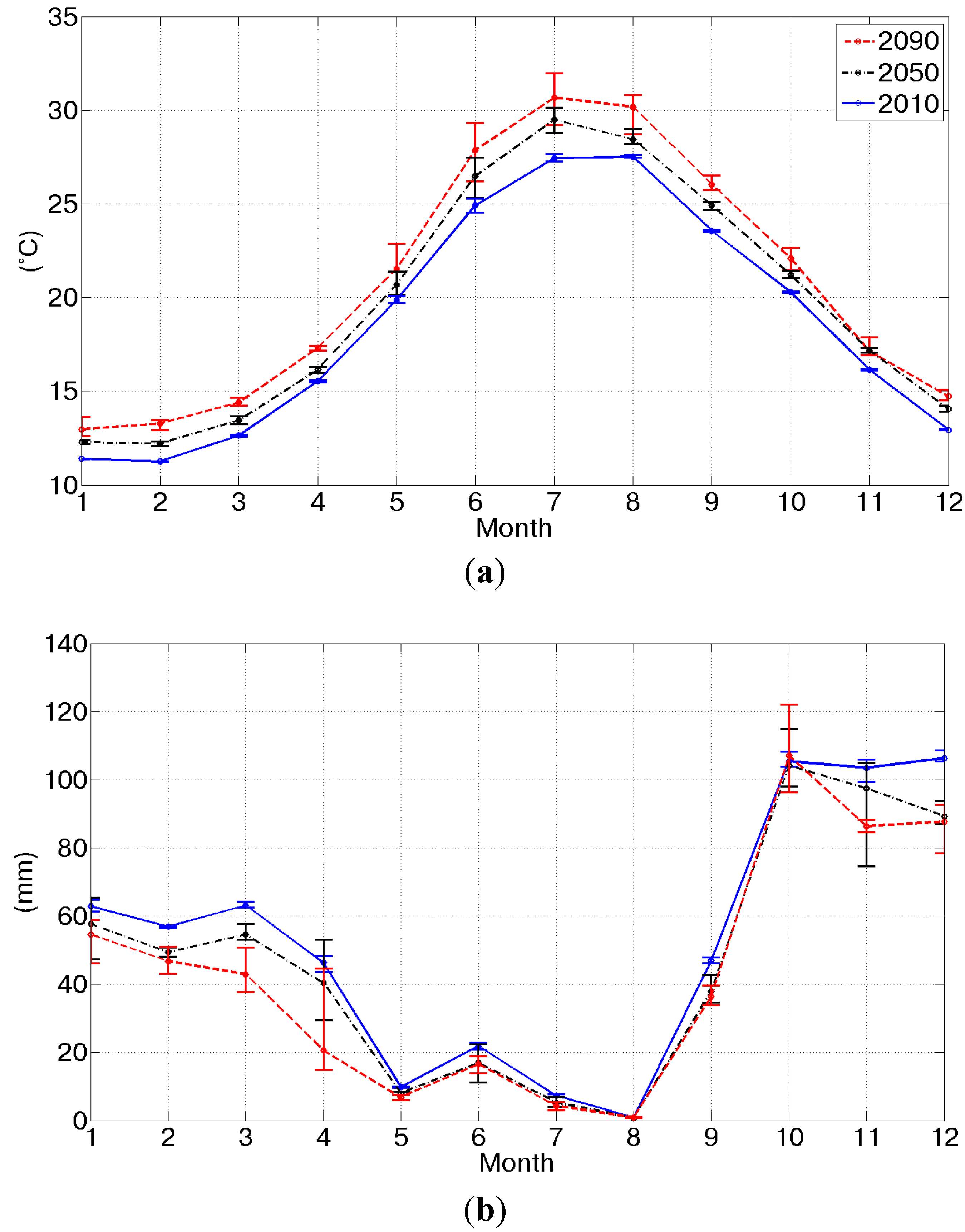
In this study, the weather generator is reparameterized using only the median of each factor of change, creating just one realization of the GCM ensemble. Figure 1 shows the monthly median of predicted future temperature and precipitation for the three considered scenarios, also including the 10–90 percentile values. As already mentioned, the interannual variability for the precipitation prediction is much higher than for air temperature. A reduction in the annual precipitation and an increase in the annual temperature can be inferred from these results, consistent with the findings of Cannarozzo et al. [42] and Viola et al. [43]. In particular, in the period 2010–2090, the mean annual precipitation decreases −123 mm and the mean annual temperature increases +2.2 °C. Significant decreases in monthly precipitation are predicted especially for March, −20.2 mm, April, −25.7 mm, November, −17.2 mm, and December, −18.7 mm. The maximum increase of temperature is predicted for the summer months, +2.9 °C in June and +3.2 °C in July; while the minimum temperature increase, +1 °C, is predicted for November.

Figure 1. The effect of the factors of change on the annual cycles of monthly temperature and precipitation. The monthly temperature (a) and precipitation (b) for the scenarios for 2010 (blue line), 2050 (black dashed line) and 2090 (red dashed line) and the 10–90 percentile intervals (vertical bars).

Figure 1. The effect of the factors of change on the annual cycles of monthly temperature and precipitation. The monthly temperature (a) and precipitation (b) for the scenarios for 2010 (blue line), 2050 (black dashed line) and 2090 (red dashed line) and the 10–90 percentile intervals (vertical bars).

Different procedures have been used to generate the future net solar radiation and wind speed series, since, as mentioned previously, factors of change for such variables were not available. Specifically, the factor of change for solar radiation has been derived from literature evidence, while the results of a trend analysis on wind speed have allowed the generation of future time series of this variable.

With regard to the solar radiation, Jiménez-Muñoz et al. [12] showed a net radiation reduction on world land of about −1 W/m² over the period 1980–2010 (−0.33 W/m² per decade). Vice versa, they demonstrated that this trend is not significant over the sea. Here, the same rate of −0.33 W/m² per decade has been assumed to occur in a constant way up to 2090. Consequently, the obtained net solar radiation decreases from 2010 (207 W/m²) to 2090 (204.3 W/m²), leading to a factor of change for each future scenario given by the ratio between future and present net solar radiation.

With regard to wind speed, a trend analysis has been performed on historical wind data collected by the Italian Air Force in order to investigate the existence of statistically significant tendencies through the Mann–Kendal test [45]. The results of such an analysis show a significant trend at the 99% confidence level with a magnitude of −0.255 m/s per decade, evaluated using the Hirsch et al. [46] estimate. This notwithstanding, wind velocity trends have been demonstrated to be highly variable in time and space within the Mediterranean basin [47]; the assumption of an average wind speed decrease, here equal to −0.255 m/s decade, is supported by a long time series analysis, which, of course, has local validity.

Finally, with regard to the relative humidity, the AWE-GEN simulated a decrease of the mean annual relative humidity from 65% in 2010 to 60% in 2090. This is due to statistical and casual relationships assumed by the AWE-GEN. The inferred change in relative humidity is mainly a result of the air temperature change.

The assumed CO₂ concentration growth affects olive physiology; in particular, olive maximum stomatal conductance has been linearly reduced, through the function, f_CO2, from 15.4 [37] to 12.32 mm·s⁻¹ in 80 years. As already mentioned, this 20% reduction is justified by several FACE experiments on a specific crops [3] and also from olive tree evidence [7]. Furthermore, when the effects of climate change on plant physiology are investigated, the conductance decrease is a common assumption [48]. Since the crop model works at the daily time scale, all these climatic data have been aggregated at such a scale and summarized in Table 1, which reports the mean annual values for the considered scenarios.

Table 1. Mean values for climatic scenarios generated by the Advanced Weather Generator (AWE-GEN) model or extrapolated by historical/literature data (italic).

Scenario	2010	2050	2090
Rain (mm/y)	649	570	526
Net Solar radiation (W/m2)	207.0	205.7	204.3
Mean Temperature (°C)	18.7	19.7	20.9
Relative humidity (%)	65	62	60
Wind speed (m/s)	4.26	3.22	2.19
CO2 (p.p.m.)	350	525	700

Table 1. Mean values for climatic scenarios generated by the Advanced Weather Generator (AWE-GEN) model or extrapolated by historical/literature data (italic).

Scenario	2010	2050	2090
Rain (mm/y)	649	570	526
Net Solar radiation (W/m2)	207.0	205.7	204.3
Mean Temperature (°C)	18.7	19.7	20.9
Relative humidity (%)	65	62	60
Wind speed (m/s)	4.26	3.22	2.19
CO2 (p.p.m.)	350	525	700

It is important to point out that the used GCM projections do not contain any information about other sources of uncertainty and are strongly affected by the hypothesized different CO₂ emission scenarios. Moreover, the variation of climate change predictions between different models is another meaningful measure of uncertainty. At the same time, however, the median factors of change between different models result, probably, in the most reliable prediction [39].

3. Results and Discussion

The model structure allows one to distinguish between a water unlimited condition, where potential fluxes are not influenced by water availability, and a soil moisture-driven condition, in which fluxes are limited by soil moisture. The first well-watered condition, even if highly unlikely in rainfed orchards, gives the opportunity for summarizing climate change effects on plant behavior, separating the water availability influence on water and CO₂ fluxes.

There are basically four main factors that drive potential evapotranspiration and assimilation. A CO₂ concentration increase determines stomatal conductance reduction and, hence, a reduction in water use. At the same time, a temperature increase makes the atmospheric water demand higher, and consequently, if it were the only climatic alteration, potential evapotranspiration would largely increase. The considered future climatic scenarios include also solar radiation and wind speed reduction: the latter acts on radiative and aerodynamic drivers of the hydrologic cycle, decreasing potential water fluxes. 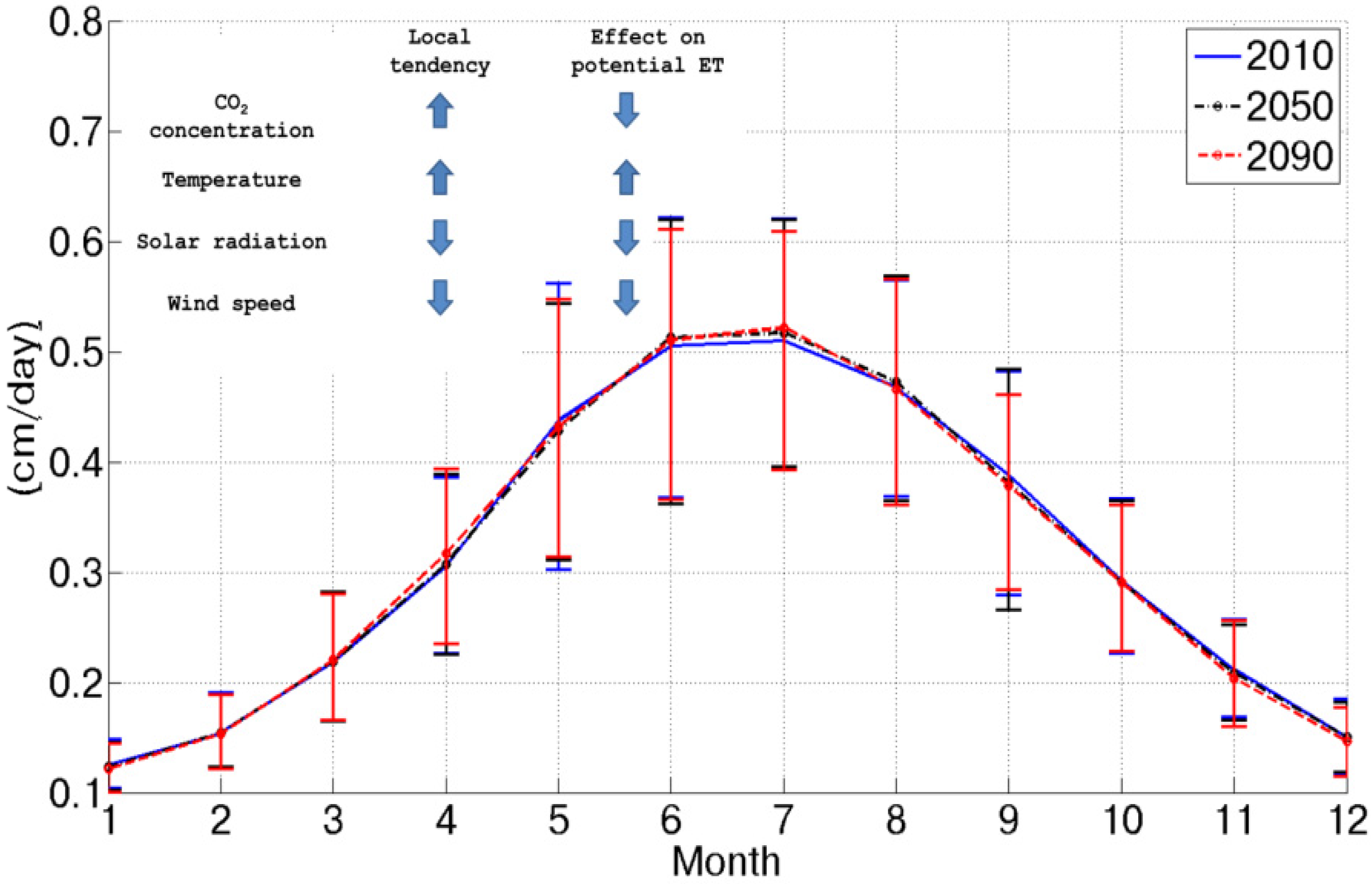Figure 2 shows the mean daily potential evapotranspiration for the three considered scenarios as obtained from the Penman–Monteith equation considering future climatic conditions as inputs. The combined effect of CO₂ concentration increase, temperature increase, wind speed decrease and net radiation decrease results in a slight potential evapotranspiration increase (+1% in the 2090 scenario). This is due to a counterbalance between causes that would increase this flux, as the temperature increase and climatic conditions and forcings, whose variation would imply a reduction (CO₂ concentration increase, solar radiation and wind speed decrease).

Figure 2. Mean daily potential evapotranspiration for each month in the three considered scenarios. The inset summarizes the local tendencies of the considered variables and the qualitative effect on potential evapotranspiration.

Figure 2. Mean daily potential evapotranspiration for each month in the three considered scenarios. The inset summarizes the local tendencies of the considered variables and the qualitative effect on potential evapotranspiration.

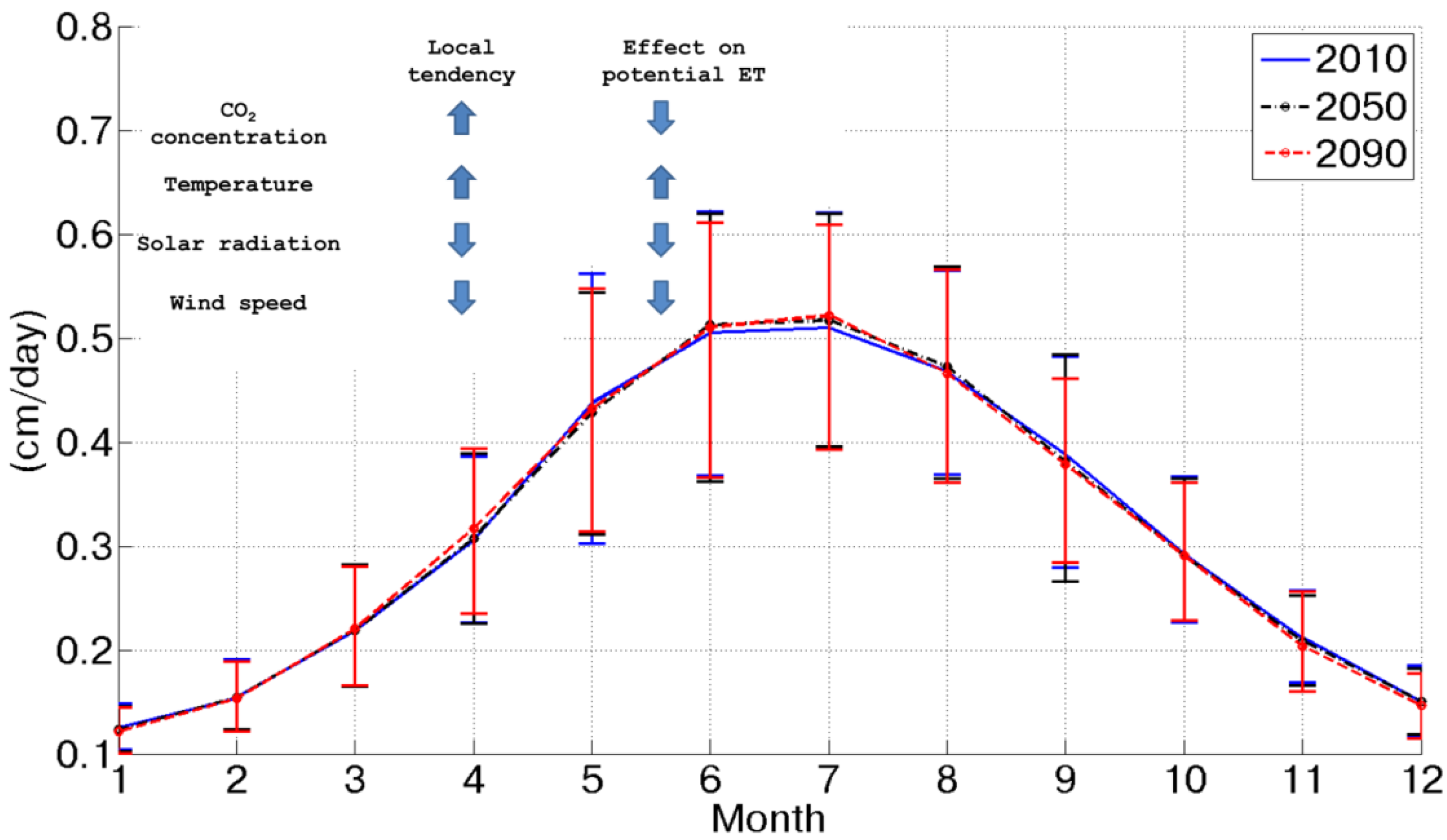
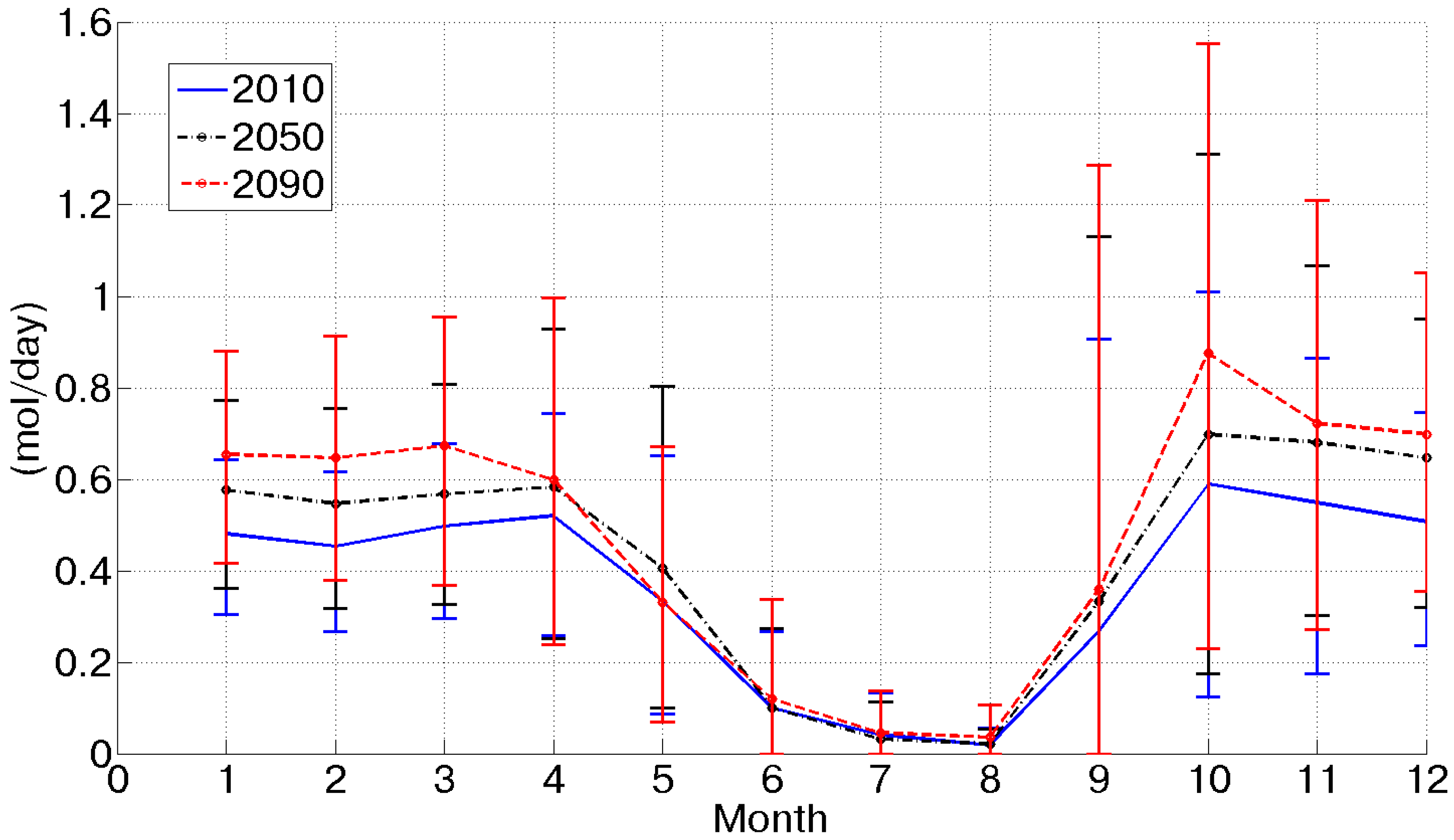
At the same time, potential assimilation experiences an important increase (more than +60% between 2010 and 2090), as shown in Figure 3. This is caused by CO₂ concentration doubling between 2010 and 2090 and a contemporary temperature increase. Considering the behavior of potential assimilation, it is possible to observe a progressive increase from the 2010 to 2090 scenario, which is amplified during the summer season, when energy is not a limiting factor, as during the winter. Of course, this forecasted tendency is intimately related and sensitive to the assumed CO₂ emission scenarios.

In order to investigate water limited conditions, soil moisture dynamics were evaluated in each considered scenario using vegetation, soil characteristics and daily climatic forcing, as given by the AWE-GEN model. It has been assumed that the initial value of soil moisture is close to the field capacity; this assumption can be considered realistic, because simulations start at the beginning of January. Moreover, this initial value does not significantly influence the final results, which are averaged over 50 years.

Figure 3. Mean daily potential assimilation for each month in the three considered scenarios.

Figure 3. Mean daily potential assimilation for each month in the three considered scenarios.

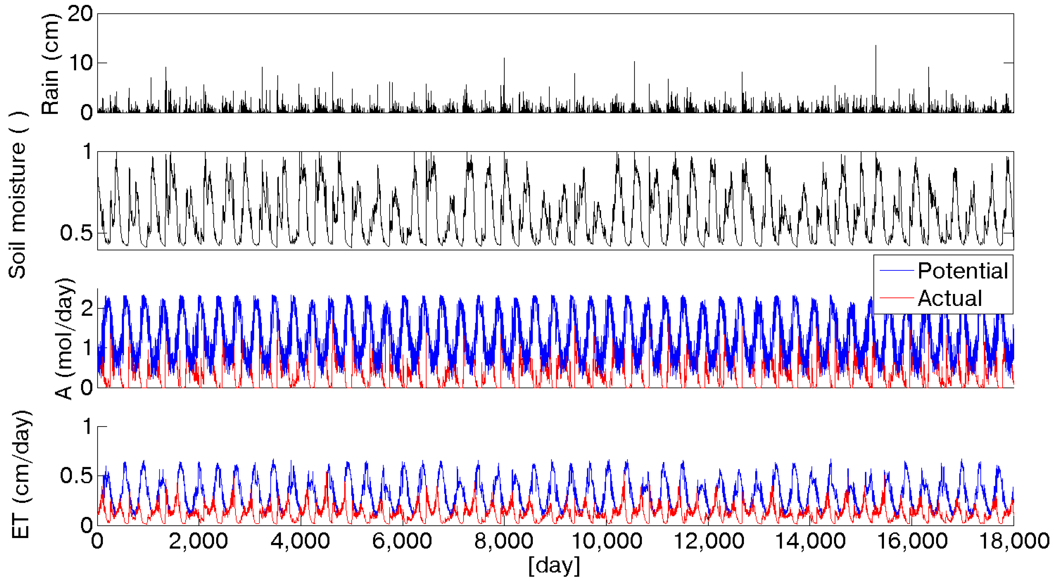
Actual evapotranspiration (ET) and assimilation (A) have been calculated at daily time scale as a function of soil moisture, as shown in Figure 4 for the 2090 scenario. A limitation induced by water availability is evident, especially during summer periods. In particular, it is possible to observe that at the beginning of the growing season, when soil moisture is still high, because of the winter recharge, evapotranspiration and assimilation are almost at their maximum level. Proceeding through the summer, the initial soil moisture is depleted, and the evapotranspirative demand continues to grow, causing an increasing gap between the potential and actual evapotranspiration and assimilation. 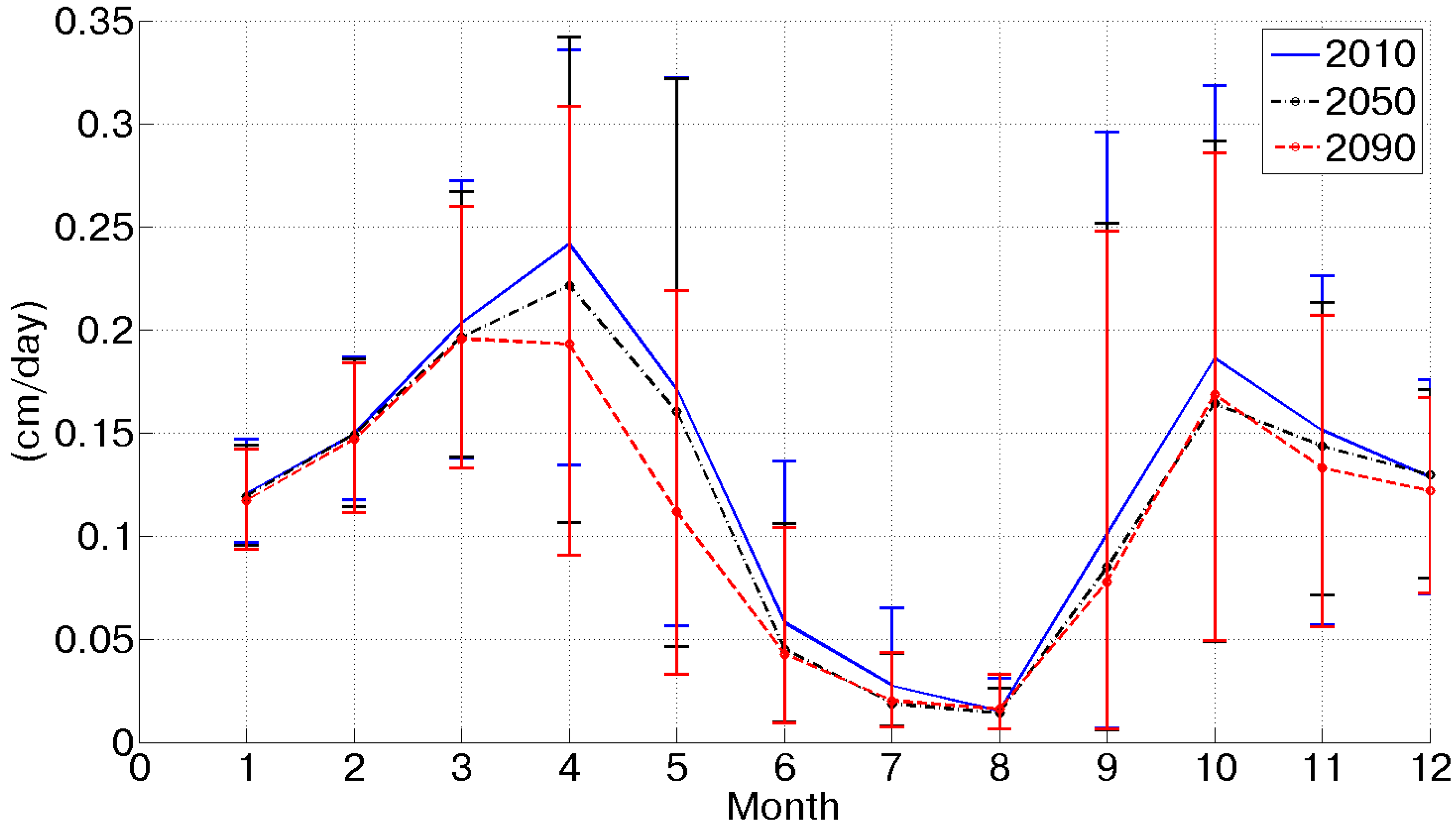Olive trees reduce their activity when this situation occurs, namely in August [49]. Usually at the beginning of September, the first autumn rainfall events occur, increasing the soil moisture content, so that trees can finalize the process of fruit development without water limitations. This alternation of dormancy and activation as a function of solar energy and soil moisture availability made the olive tree one of the best adapted species in Mediterranean ecosystems. It is interesting to compare the annual values of potential evapotranspiration and assimilation with the actual values under limited water availability conditions. The reduced rainfall input is reflected in soil moisture dynamics and, in turn, it affects evapotranspiration and assimilation rates. Because of the water availability reduction, evapotranspiration decreases from the current scenario to the 2090, from about 470 to 400 mm. An overall view of evapotranspiration limited by soil moisture availability is depicted in Figure 5 where the progressive reduction over the considered scenarios is represented by the downshifting of the curves ranging from the 2010 to the 2090 scenario. The seasonal traces of the mean daily actual evapotranspiration show two peaks, instead of the unique maximum characterizing potential fluxes (Figure 2), one during the spring and the second in the fall, coherently with soil moisture dynamics.

Figure 4. 50 years of daily stochastic rainfall and soil moisture series in the 2090 scenario. The two bottom rows show the comparison between potential (blue line) and water limited (red line) assimilation and evapotranspiration.

Figure 4. 50 years of daily stochastic rainfall and soil moisture series in the 2090 scenario. The two bottom rows show the comparison between potential (blue line) and water limited (red line) assimilation and evapotranspiration.

Figure 5. Mean daily actual evapotranspiration for each month limited by soil moisture availability in the three considered scenarios.

Figure 5. Mean daily actual evapotranspiration for each month limited by soil moisture availability in the three considered scenarios.

A similar behavior can be observed for actual assimilation (Figure 6). Interestingly, because of the increased potential assimilation, the actual assimilation grows from 2010 to 2090, as well. Soil moisture limitations during the summer make the actual assimilation differences in these months not relevant among the three scenarios; but an evident increase from 2010 to 2090 can be noticed in the September–October period, when the first rainfall events after the dry season occur.

Figure 6. Mean daily actual assimilation for each month limited by soil moisture availability in the three considered scenarios.

Figure 6. Mean daily actual assimilation for each month limited by soil moisture availability in the three considered scenarios.

Integrating actual assimilation over the vegetative growth period, which lasts for five months from June to November [49], it is possible to obtain the olive yield for each year within the considered scenario. It is worth noticing that annual yield is also influenced by the dynamic water stress [26] computed during the same year. The average values of this index vary in the three considered scenarios. It increases (from 0.52 in 2010 to 0.63 in 2090), because of more prolonged periods with soil moisture traces below the stomatal closure point as rainfall decreases; this behavior, in turn, influences the biomass partitioning according to Equation (6). Average values obtained in the three considered scenarios are reported in Table 2. The simulated olive yield amounts to 27 ql/ha in the 2010 scenario and progressively increases to 31 ql/ha in the 2090 scenario. The growth of productivity equal to about 14% in 80 years reflects the effects of the CO₂ concentration increase, but strongly smoothed by the rainfall reduction (−20%), which imposes a soil moisture limitation to transpiration and assimilation over the growing season.

Table 2. Modeled mean values in the three considered scenarios.

Scenario	2010	2050	2090
Potential ET (mm/y)	1135	1140	1146
Actual ET (mm/y)	472	440	409
Potential Assimilation (mol/m2)	0.80	1.08	1.32
Actual Assimilation (mol/m2)	0.37	0.43	0.48
Olive yield (ql/ha)	27.39	29.90	31.32

Table 2. Modeled mean values in the three considered scenarios.

Scenario	2010	2050	2090
Potential ET (mm/y)	1135	1140	1146
Actual ET (mm/y)	472	440	409
Potential Assimilation (mol/m2)	0.80	1.08	1.32
Actual Assimilation (mol/m2)	0.37	0.43	0.48
Olive yield (ql/ha)	27.39	29.90	31.32

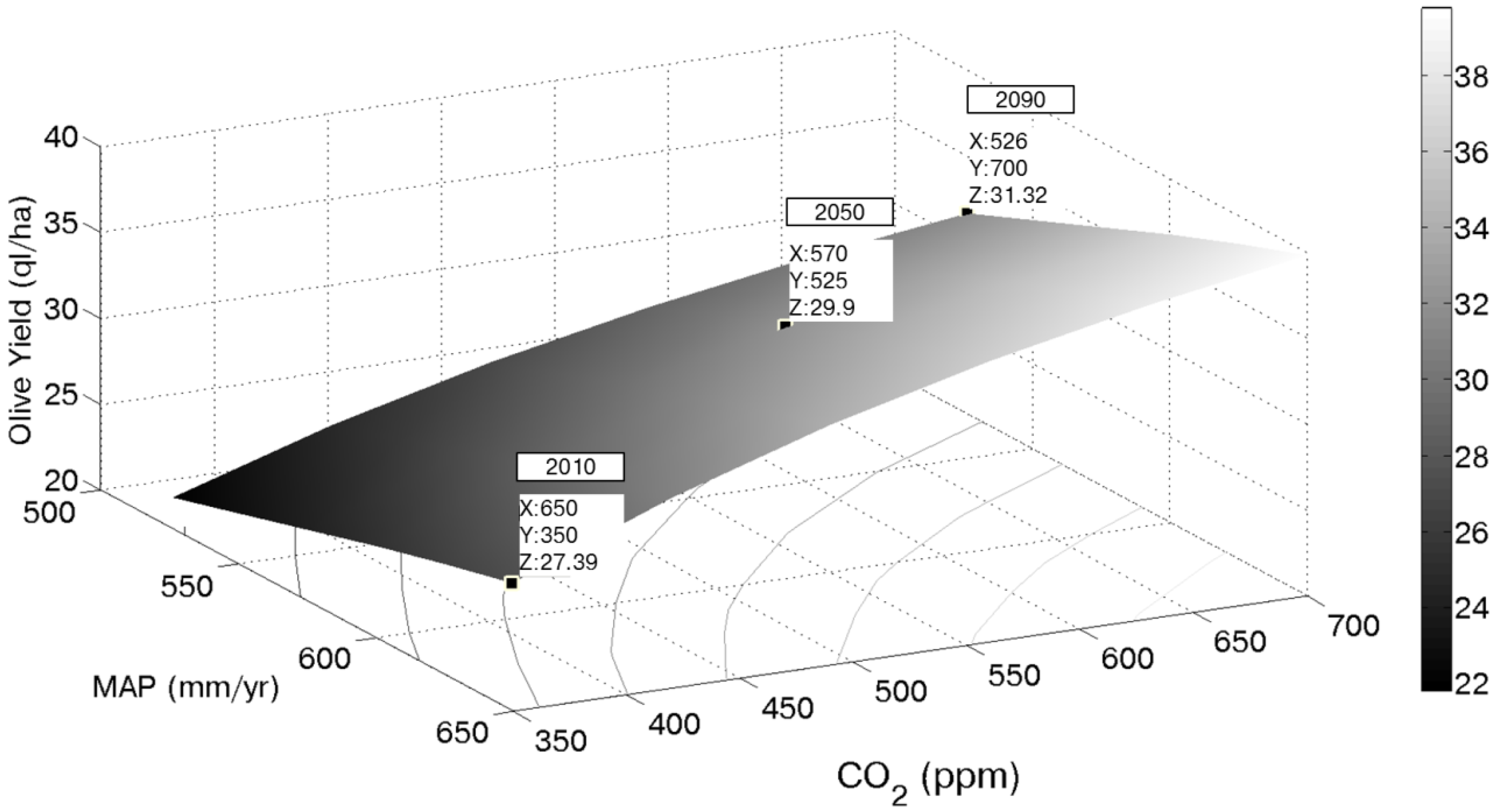
In order to give a wider view of the effect of the change of the main factors driving olive yield, the relationship among mean annual precipitation (MAP), CO₂ concentration and productivity has been investigated. The same three climate scenarios (2010, 2050 and 2090) obtained by the AWE-GEN model have been used. For each of the three climatic scenarios, the crop model has been run using ten different CO₂ concentrations varying from 350 to 700 ppm. These new model runs have provided thirty time series of olive productivity (ten for each climatic scenario). The thirty mean annual values of olive yield have been calculated from these time series and then interpolated as a function of MAP and CO₂ concentration to obtain the surface depicted in Figure 7 (or the isolines shown in the same figure). It is worth pointing out that just three points of such a surface can be considered as coherent with CO₂ scenarios and the corresponding GCMs’ rainfall forecast; namely, these three points correspond to the climatic scenarios summarized in Table 1.

Figure 7. Mean annual olive yields as a function of CO₂ concentration and mean annual precipitation (MAP). Results in the three considered future scenarios are highlighted. Iso-productivity lines are projected using the gray scale on the right.

Figure 7. Mean annual olive yields as a function of CO₂ concentration and mean annual precipitation (MAP). Results in the three considered future scenarios are highlighted. Iso-productivity lines are projected using the gray scale on the right.

A careful analysis of this figure shows that, keeping the current value of CO₂ concentration and reducing the annual rainfall, one could observe an olive yield reduction, coherently with the results shown by Viola et al. [50]. On the contrary, if the annual rainfall would remain constant and the CO₂ concentration would increase, olive yield could benefits from such a condition. The latter two behaviors give the opportunity of explaining the main drivers that determine an increase in olive yield in the considered scenarios. The CO₂ concentration increase would increase olive yield, but the water availability limitation controls and limits this tendency. As stated before, the productivity dynamics may be considered representative for a wide area located in the Northwest of the island. In the next 80 years, the model predicts an olive yield increase of about 4 ql/ha. Using a constant ratio between oil and fruits (one liter for seven kilos of fruits) and assuming as fixed the current price for olive oil (5 €/liter) the gross income for the whole Trapani province’s orchards could increase from about 50 to 56 M€. Of course, this result is influenced, besides the assumptions related to the CO₂ scenarios and to the uncertainties characterizing the GCM projections, also by the market dynamics, which can be even more unclear.

4. Conclusions

The interrelations between future climate scenarios and olive yield have been investigated for a Mediterranean orchard. The ecohydrological model used here emphasizes the fundamental processes involved in crop productivity and the dependencies on water deficits, both from a physiological and an agronomic perspective.

Three climate scenarios downscaled from an ensemble of climate model outputs, using the AWE-GEN weather generator, have been investigated. The impacts of the main local likely climatic modifications, namely the CO₂ concentration increase, the temperature increase, the net radiation decrease, the wind speed reduction and the rainfall decrease, have been investigated. The computation of potential fluxes, with full soil water availability, showed a slightly increase in potential transpiration, because different climatic tendencies can counterbalance each other, and a massive increase in potential assimilation. At the same time, potential assimilation encounters an increase mainly driven by the CO₂ concentration increase.

In order to account for water availability, evapotranspiration and assimilation have been assessed by a stepwise function of soil moisture at the daily time scale. Then, assimilation rates over the olive growth period have been obtained, integrating carbon and partitioning the biomass as a function of vegetation water stress.

Results are justified by the drought tolerance of olive trees, showing a local increase in olive yield for the considered scenarios, mostly due to the potential assimilation increase mitigated by rainfall reduction. The diminished water input affects soil moisture dynamics, which, in turn, limits evapotranspiration and assimilation. Furthermore, the vegetation water stress increase modifies the amount of carbon allocated in fruit production, implying a non-constant ratio between transpiration and yield.

A rough economic analysis has linked the increase in productivity with the local farmers’ gross income increase. This result deserves further attention for including the relationships linking vegetation water stress with oil quality and to reduce the uncertainties arising from CO₂ emission scenarios and the GCMs’ outputs.