Inexact Mathematical Modeling for the Identification of Water Trading Policy under Uncertainty

Abstract
:1. Introduction
2. Methodology

 is the expected value of the second-stage penalties [12]. However, the parameter of a model may fluctuate within a certain interval, and it is difficult to state a meaningful probability distribution for this variation. Interval-parameter programming (IPP) can deal with uncertainties in objective function and system constraints, which can be expressed as intervals without distribution information. An interval number, x±, can be defined as an interval with a known lower-bound and upper-bound, but unknown distribution information [34,35]. It can be expressed as [x−, x+], representing a number (or an interval), which can have a minimum value of x− and a maximum one of x+.


 be a fuzzy set of imprecise right-hand sides with possibility distributions. The triangular fuzzy membership function is the most popular possibility distribution, and it is adopted in this study, due to its computational efficiency. Accordingly, the credibility of the constraint Ax ≤ could be defined as follows [32]:


 when
when  ,
,  when
when  and λ- = the lower bound of the credibility level value.
  for j = 1 to q1,
  for j = q1 + 1 to n,
  for k = 1 to q2 and
  for k = q2 + 1 to m, can be obtained. Accordingly, the second submodel corresponding to the lower bound of the objective function value can be formulated as:


 for j = 1 to q1, for j = q1 + 1 to n, for k = 1 to q2 and for k = q2 + 1 to m. Therefore, by integrating the solutions of the two submodels, the solution of the TICP model can be generated.
- Step 1: Formulate the TICP model.
- Step 2: Transform the TICP model into two submodels, where the submodel corresponding to ƒ+ is desired first, since the objective is to maximize ƒ±.
- Step 3: Obtain the optimal solutions by solving the ƒ+ submodel under each λ.
- Step 4: Formulate and solve the ƒ- submodel by importing optimal solutions from the ƒ+ submodel into the ƒ-submodel under each λ.
- Step 5: Obtain the optimal solution interval value under each λ.
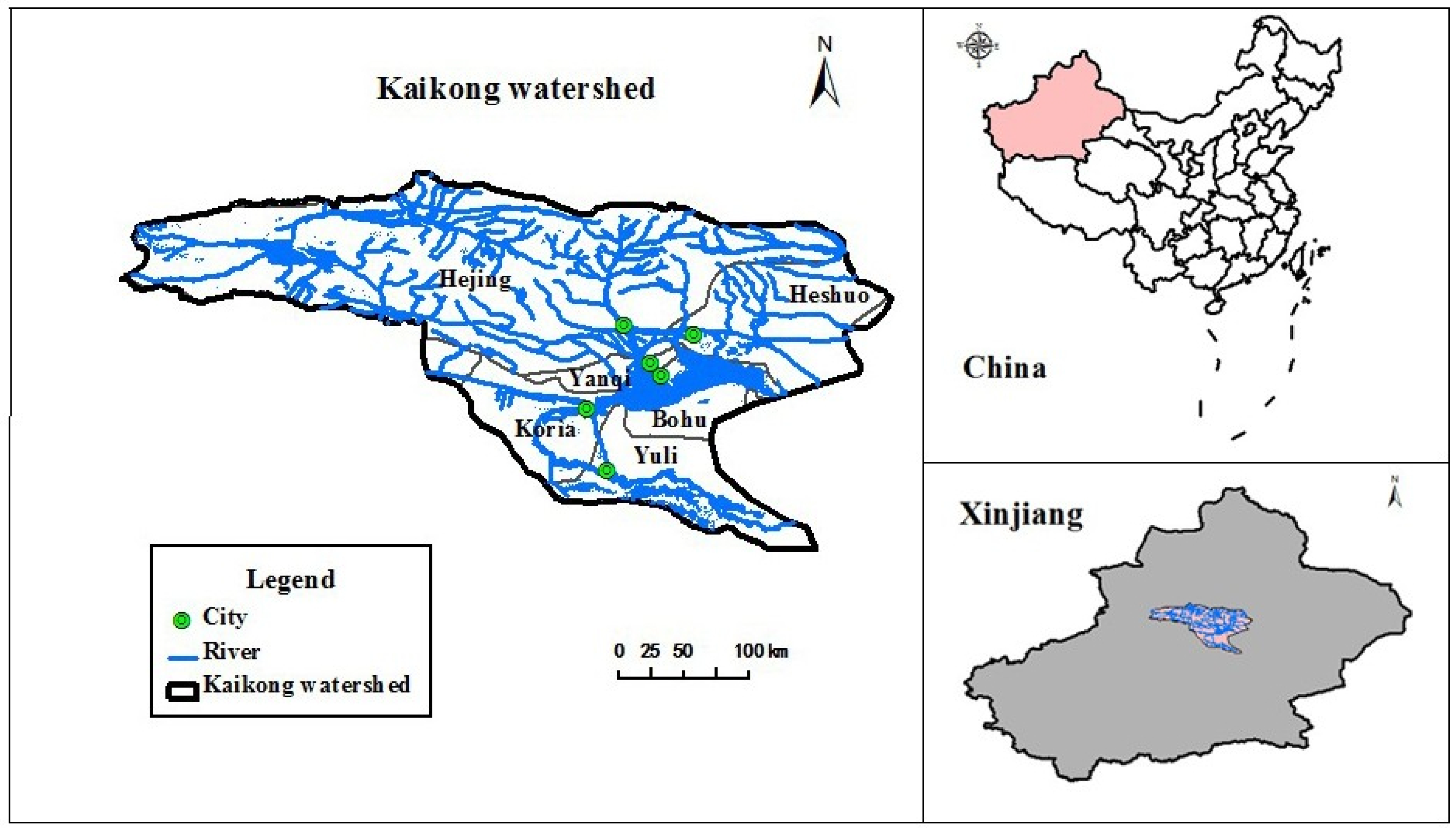
3. Case Study

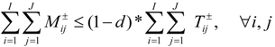
- (1)
- Constraints of water permit:
![Water 06 00229 i028]()
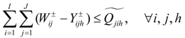
- (2)
- Constraints of water shortage:
![Water 06 00229 i029]()
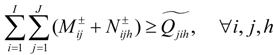
- (3)
- Constraints of water surplus:
![Water 06 00229 i030]()
- (4)
- Constraints of water trading:
![Water 06 00229 i031]()
![Water 06 00229 i032]()
- (5)
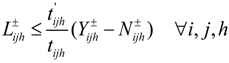
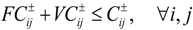
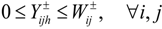
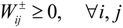
- Constraints of technical:
![Water 06 00229 i033]()
![Water 06 00229 i034]()
![Water 06 00229 i035]()

 presents the net benefit of the entire system with trading (US$),
  is net benefit to user i in district j per volume of water being delivered (US$/103 m3),
  is the water demand target for user i in district j (106 m3),
  is the total water availability of the entire system under probability Ph (106 m3), Ph denotes the probability of random water availability
  under level h (%),
  is the economic loss to user i in district j per volume of water not being delivered (US$/103 m3),
  is the water deficiency for user i in district j when demand is not met (106 m3),
  is the allocated allowable water permit to user i in district j (106 m3), λ is the credibility level, which measures the degrees of satisfaction of the constraints, d is the percentage of the reduced total allowable water allocation,
  is the water released to user i in district j when the total water availability exceeds the allowable water reallocation with trading scheme (106 m3),
  is the trading fixed cost to user i in district j with trading scheme (US$/103 m3),
  is the variable trading cost to user i in district j with trading scheme (US$/103 m3),
  is the amount of water trading from other water sources to user i in district j with trading scheme (106 m3) and tʹijh / tijh is the ratio of water trading from other water sources to user i in district j with the trading scheme. and are estimated according to different users’ gross national product in different counties indirectly, the upper bound values of which are estimated as the highest from the yearbook (2005–2010) and the lower bound values of which are the opposite. For example, the net benefit ( ) for the agricultural user in Hejing County is estimated by the gross amount of crops (i.e., wheat, corn, tomato, cotton and fruit) and the total water demand (net benefit = gross amount of crops/total water demand). From 2005 to 2010, the highest net benefit was 1860 US$/103 m3 in 2008, which was estimated by the gross amount of crops (i.e., wheat = 45.1 × 10⁶ US$; oil plant = 11.3 × 10⁶ US$; tomato = 15.93 × 10⁶ US$; cotton t = 44.02 × 10⁶ US$ and other crops = 47.33 × 10⁶ US$) and the water demand (i.e., wheat = 24.1 × 10⁶ m3; oil plant = 2.91 × 10⁶ m3; tomato = 3.41 × 10⁶ m3; cotton = 29.4 × 10⁶ m3 and other crops = 28.18 × 10⁶ m3). Meanwhile, the lowest net benefit was 1530 US$/103 m3 in 2005. Therefore, the interval value of the net benefit is acquired as [1530, 1860] US$/103 m3, which is on the basis of the highest and lowest value of the net benefit. The method calculated for the net benefit of the agricultural user in Hejing County can be applied to other users, districts and even other economic data. is a basic form of trading cost, which is estimated by the actual price of water exceed water permit in Kaidu-kongque Basin. is estimated according to the opportunity cost of water, which is affected by a number of factors, such as the scarcity of water resources, the relationship between supply and demand and the status of socio-economic development. Table 2 shows policy data , which are acquired from the water permits of the water authority of Uygur Autonomous Region from 2005 to 2010 directly. Additionally, water target is estimated by the users’ actual water usage in recent years, which takes the situation of economic development into consideration. The value of should be derived by conducting statistical analyses with the results of the annual streamflow of the Kaidu-kongque River (2005–2010). Due to the rainy seasons in the Kaidu-kongque River Basin, more than 80% of the total annual precipitation falls from May to September, and less than 20% of the total falls from November to the following April [37]. Therefore, the total water availability can be converted to several levels. Table 3 shows the total water availability of the Kaidu-kongque River Basin under several level probabilities. and are estimated according to different users’ gross national product in different counties indirectly, the upper bound values of which are estimated as the highest from the yearbook (2005–2010) and the lower bound values of which are the opposite. For example, the net benefit ( ) for the agricultural user in Hejing County is estimated by the gross amount of crops (i.e., wheat, corn, tomato, cotton and fruit) and the total water demand (net benefit = gross amount of crops/total water demand). From 2005 to 2010, the highest net benefit was 1860 US$/103 m3 in 2008, which was estimated by the gross amount of crops (i.e., wheat = 45.1 × 10⁶ US$; oil plant = 11.3 × 10⁶ US$; tomato = 15.93 × 10⁶ US$; cotton t = 44.02 × 10⁶ US$ and other crops = 47.33 × 10⁶ US$) and the water demand (i.e., wheat = 24.1 × 10⁶ m3; oil plant = 2.91 × 10⁶ m3; tomato = 3.41 × 10⁶ m3; cotton = 29.4 × 10⁶ m3 and other crops = 28.18 × 10⁶ m3). Meanwhile, the lowest net benefit was 1530 US$/103 m3 in 2005. Therefore, the interval value of the net benefit is acquired as [1530, 1860] US$/103 m3, which is on the basis of the highest and lowest value of the net benefit. The method calculated for the net benefit of the agricultural user in Hejing County can be applied to other users, districts and even other economic data. is a basic form of trading cost, which is estimated by the actual price of water exceed water permit in Kaidu-kongque Basin. is estimated according to the opportunity cost of water, which is affected by a number of factors, such as the scarcity of water resources, the relationship between supply and demand and the status of socio-economic development. Table 2 shows policy data , which are acquired from the water permits of the water authority of Uygur Autonomous Region from 2005 to 2010 directly. Additionally, water target is estimated by the users’ actual water usage in recent years, which takes the situation of economic development into consideration. The value of should be derived by conducting statistical analyses with the results of the annual streamflow of the Kaidu-kongque River (2005–2010). Due to the rainy seasons in the Kaidu-kongque River Basin, more than 80% of the total annual precipitation falls from May to September, and less than 20% of the total falls from November to the following April [37]. Therefore, the total water availability can be converted to several levels. Table 3 shows the total water availability of the Kaidu-kongque River Basin under several level probabilities.
| District | User | |||
|---|---|---|---|---|
| i = 1 | i = 2 | i = 3 | i = 4 | |
| Municipality | Agriculture | Industry | Ecology | |
| Net benefits (unit: US$/103 m3) | ||||
| j = 1 Kuerle county | [6030, 6670] | [2320, 2520] | [4530, 4670] | [1960, 2120] |
| j = 2 Yanqi county | [5500, 6040] | [1420, 1560] | [2600, 2930] | [1680, 1930] |
| j = 3 Hejing county | [4670, 4800] | [1530, 1860] | [3730, 3810] | [1540, 1780] |
| j = 4 Heshuo county | [5300, 5530] | [2010, 2340] | [3440, 3620] | [1660, 1940] |
| j = 5 Bohu county | [4910, 5100] | [1780, 2010] | [3620, 3740] | [1530, 1840] |
| j = 6 Yuli county | [4600, 5260] | [2230, 2460] | [3220, 3440] | [1690, 1990] |
| Penalties (unit: US$/103 m3) | ||||
| j = 1 Kuerle county | [9045, 10005] | [3480, 3765] | [6795, 7005] | [2940, 3180] |
| j = 2 Yanqi county | [8250, 9060] | [2130, 2340] | [3900, 4395] | [2520, 2895] |
| j = 3 Hejing county | [7005, 7200] | [2295, 2790] | [5595, 5725] | [2310, 2670] |
| j = 4 Heshuo county | [7950, 8295] | [3015, 3510] | [5160, 5430] | [2190, 2490] |
| j = 5 Bohu county | [7365, 7650] | [2670, 3015] | [5430, 5610] | [2295, 2760] |
| j = 6 Yuli county | [6900, 7890] | [3345, 3690] | [4830, 5160] | [2535, 2985] |
| Trading fix cost (unit: US$/103 m3) | ||||
| j = 1 to 6 | [3050, 3150] | [550, 650] | [2400, 2600] | [280, 350] |
| Trading variable cost (unit: US$/103 m3) | ||||
| j = 1 to 6 | [1200, 1350] | [700, 800] | [150, 200] | [100, 150] |
| District | User | |||
|---|---|---|---|---|
| i = 1 | i = 2 | i = 3 | i = 4 | |
| Municipality | Agriculture | Industry | Ecology | |
| Water target (unit: 106 m3) | ||||
| j = 1 Kuerle County | [8.80, 14.00] | [258.00, 275.00] | [53.30, 620.00] | [56.00, 76.00] |
| j = 2 Yanqi County | [6.00, 8.20] | [158.00, 165.00] | [28.00, 39.00] | [31.00, 47.00] |
| j = 3 Hejing County | [2.40, 4.30] | [81.00, 88.00] | [16.00, 20.10] | [14.70, 23.00] |
| j = 4 Heshuo County | [0.24, 0.50] | [9.70, 10.10] | [1.78, 2.25] | [1.28, 2.60] |
| j = 5 Bohu County | [2.20, 4.30] | [75.00, 85.00] | [15.60, 19.00] | [13.70, 23.00] |
| j = 6 Yuli County | [4.60, 6.00] | [110.00, 120.00] | [21.60, 27.00] | [24.00, 33.00] |
| Allocated allowable water permit (unit: 106 m3) | ||||
| j = 1 Kuerle County | [9.72, 13.75] | [261.60, 275.08] | [55.44, 61.89] | [59.56, 75.65] |
| j = 2 Yanqi County | [[6.64, 8.14] | [158.33, 162.87] | [30.31, 36.65] | [32.26, 44.79] |
| j = 3 Hejing County | [2.89, 4.23] | [82.22, 84.50] | [15.70, 19.01] | [17.08, 23.24] |
| j = 4 Heshuo County | [0.36, 0.53] | [9.11, 9.38] | [1.89, 2.11] | [1.69, 2.70] |
| j = 5 Bohu County | [2.56, 4.09] | [78.89, 81.84] | [15.78, 18.41] | [15.58, 22.58] |
| j = 6 Yuli County | [4.94, 5.87] | [110.56, 117.41] | [22.33, 26.42] | [25.56, 32.29] |
| District | Level | Probability | User | |||
|---|---|---|---|---|---|---|
| i = 1 | i = 2 | i = 3 | i = 4 | |||
| Municipality | Agriculture | Industry | Ecology | |||
| Total water availability (unit: 106 m3) | ||||||
| j = 1 Kuerle County | h = 1 (low) | 0.6 | [6.57, 10.67] | [202.32, 216.00] | [43.47, 49.96] | [42.30, 58.50] |
| h = 2 (medium) | 0.3 | [7.30, 11.85] | [224.80, 240.00] | [48.30, 55.51] | [47.00, 65.00] | |
| h = 3 (high) | 0.1 | [8.03, 13.04] | [247.28, 264.00] | [53.13, 61.06] | [51.70, 71.50] | |
| j = 2 Yanqi County | h = 1 (low) | 0.6 | [4.77, 6.38] | [124.02, 128.70] | [22.86, 29.41] | [22.95, 35.55] |
| h = 2 (medium) | 0.3 | [5.30, 7.09] | [137.80, 143.00] | [25.40, 32.68] | [25.50, 39.50] | |
| h = 3 (high) | 0.1 | [5.83, 7.80] | [151.58, 157.30] | [27.94, 35.95] | [28.05, 43.45] | |
| j = 3 Hejing County | h = 1 (low) | 0.6 | [1.89, 3.24] | [66.11, 68.40] | [12.96, 16.29] | [11.43, 17.82] |
| h = 2 (medium) | 0.3 | [2.10, 3.60] | [73.45, 76.00] | [14.40, 18.10] | [12.70, 19.80] | |
| h = 3 (high) | 0.1 | [2.31, 3.96] | [80.80, 83.60] | [15.84, 19.91] | [13.97, 21.78] | |
| j = 4 Heshuo County | h = 1 (low) | 0.6 | [0.19, 0.38] | [7.90, 8.19] | [1.40, 1.62] | [0.88, 1.90] |
| h = 2 (medium) | 0.3 | [0.21, 0.42] | [8.78, 9.10] | [1.55, 1.80] | [0.98, 2.11] | |
| h = 3 (high) | 0.1 | [0.23, 0.46] | [9.66, 10.01] | [1.71, 1.98] | [1.08, 2.32] | |
| j = 5 Bohu County | h = 1 (low) | 0.6 | [1.79, 3.33] | [58.50, 65.70] | [12.69, 15.38] | [11.16, 18.20] |
| h = 2 (medium) | 0.3 | [1.99, 3.70] | [65.00, 73.00] | [14.10, 17.09] | [12.40, 20.23] | |
| h = 3 (high) | 0.1 | [2.19, 4.07] | [71.50, 80.30] | [15.51, 18.80] | [13.64, 22.25] | |
| j = 6 Yuli County | h = 1 (low) | 0.6 | [3.69, 4.75] | [86.85, 93.82] | [17.64, 21.79] | [19.35, 26.10] |
| h = 2 (medium) | 0.3 | [4.10, 5.28] | [96.50, 104.25] | [19.60, 24.21] | [21.50, 29.00] | |
| h = 3 (high) | 0.1 | [4.51, 5.81] | [106.15, 114.67] | [21.56, 26.63] | [23.65, 31.90] | |
4. Result Analysis
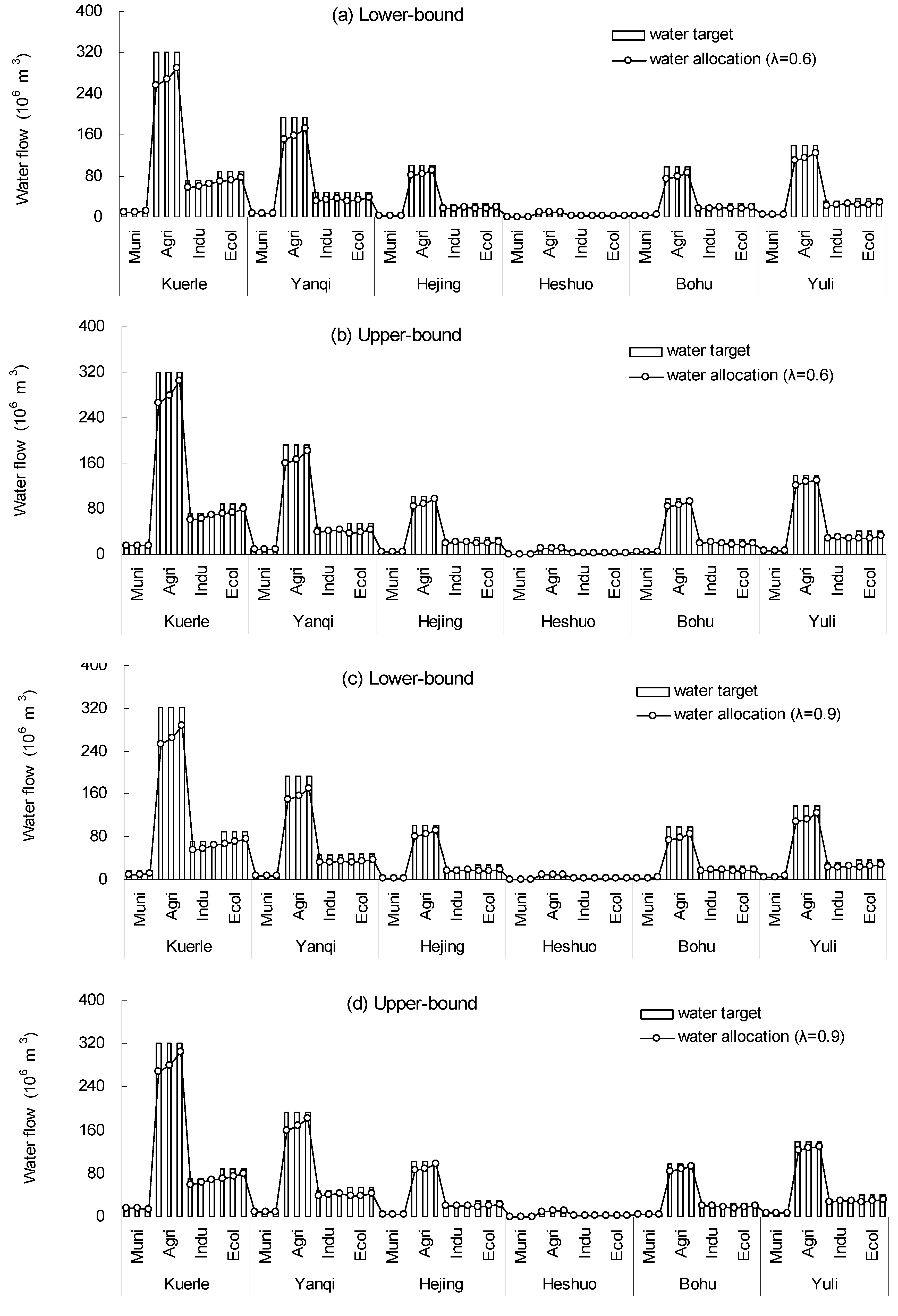
4.1. Results under Different Credibility Levels


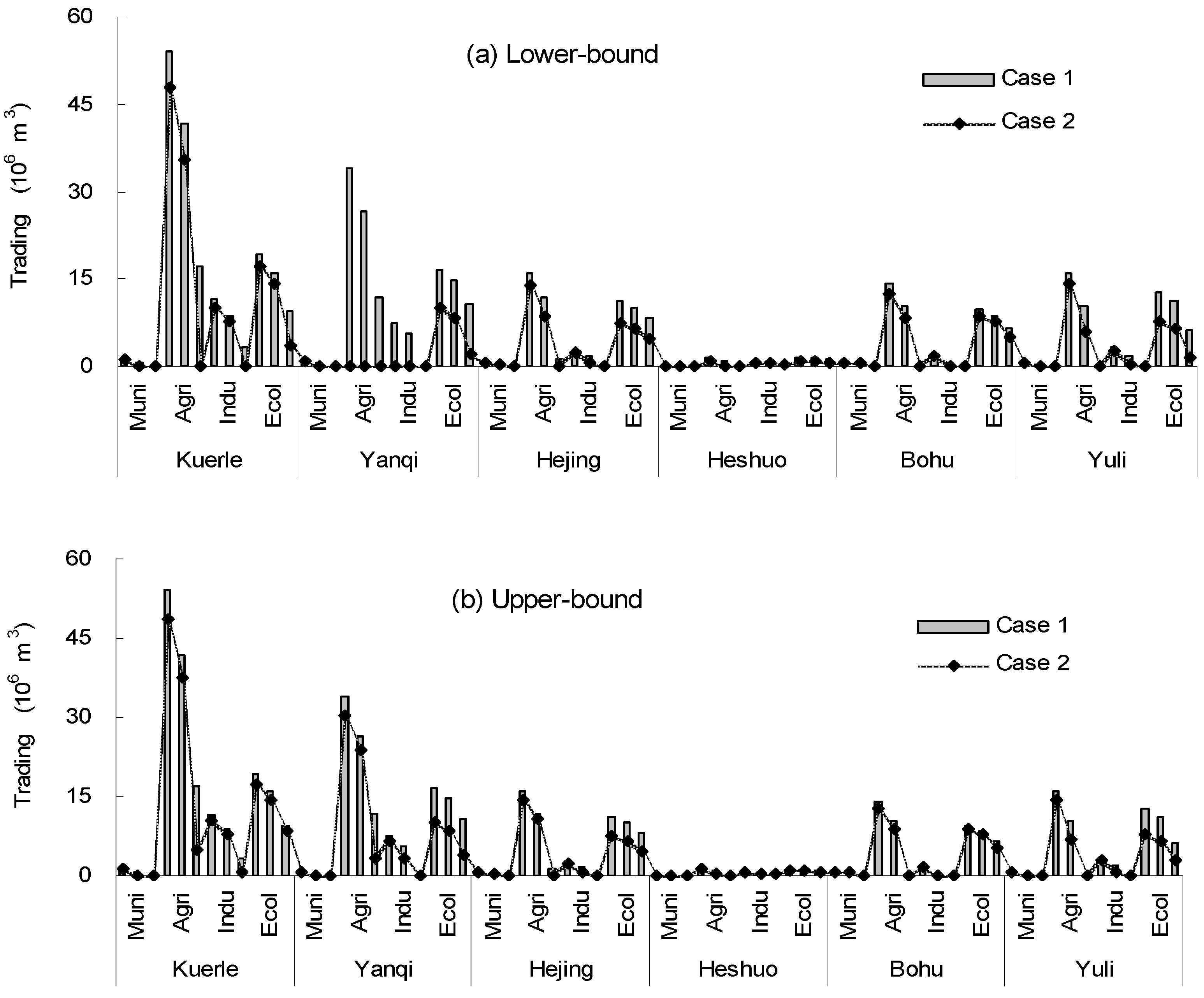
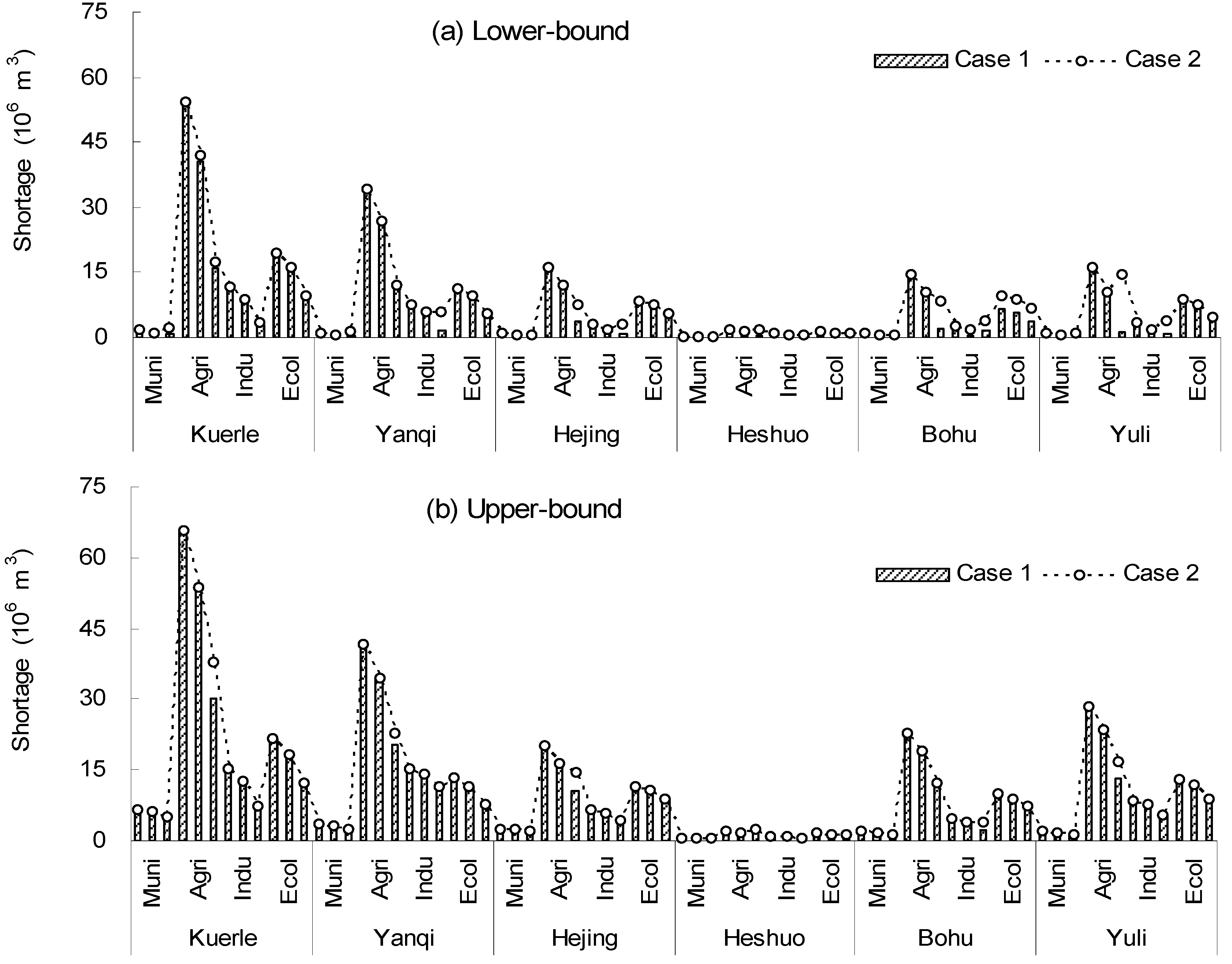
4.2. Comparison of Trading and Non-Trading Schemes


5. Conclusions
Acknowledgments
Conflicts of Interest
References
- Bates, B.C.; Kundzewicz, Z.W.; Wu, S.; Palutikof, J.P. Climate Change and Water. In Technical Paper of the Intergovernmental Panel on Climate Change; IPCC Secretariat: Geneva, Switzerland, 2008. [Google Scholar]
- Huang, Y.; Li, Y.P.; Chen, X.; Ma, Y.G. Optimization of irrigation water resources for agricultural sustainability in Tarim River Basin, China. Agric. Water Manag. 2012, 107, 74–85. [Google Scholar] [CrossRef]
- Hassan, Q.K.; Sekhon, N.S.; Magai, R.; McEachern, P. Reconstruction of snow water equivalent and snow depth using remote sensing data. J. Environ. Inform. 2012, 20, 67–74. [Google Scholar]
- Su, L.Y.; Christensen, P.; Liu, J.L. Comparative study of water resource management and policies for ecosystems in China and Denmark. J. Environ. Inform. 2013, 21, 72–83. [Google Scholar] [CrossRef]
- Calatrava, J.; Garrido, A. Spot water markets and risk in water supply. Agric. Econ. 2005, 33, 131–143. [Google Scholar] [CrossRef]
- Zaman, A.M.; Malano, H.M.; Davidson, B. An integrated water trading–allocation model, applied to a water market in Australia. Agric. Water Manag. 2009, 96, 149–159. [Google Scholar] [CrossRef]
- Youkhana, E.; Laube, W. Virtual water trade: A realistic policy option for the countries of the Volta Basin in West Africa? Water Policy 2009, 11, 569–581. [Google Scholar] [CrossRef]
- Luo, B.; Maqsood, I.; Gong, Y.Z. Modeling climate change impacts on water trading. Sci. Total Environ. 2010, 408, 2034–2041. [Google Scholar] [CrossRef]
- Dominguez, D.; Truffer, B.; Gujer, W. Tackling uncertainties in infrastructure sectors through strategic planning: The contribution of discursive approaches in the urban water sector. Water Policy 2010, 13, 299–316. [Google Scholar] [CrossRef]
- Li, Y.P.; Huang, G.H.; Chen, X. Multistage scenario-based interval-stochastic programming for planning water resources allocation. Stoch. Environ. Res. Risk Assess. 2009, 23, 781–792. [Google Scholar] [CrossRef]
- Ahmed, S.; Tawarmalani, M.; Sahinidis, N.V. A finite branch-and-bound algorithm for two-stage stochastic integer programs. Math. Program. 2004, 100, 355–377. [Google Scholar] [CrossRef]
- Li, Z.; Huang, G.; Zhang, Y.; Li, Y. Inexact two-stage stochastic credibility constrained programming for water quality management. Resourc. Conserv. Recycl. 2013, 73, 122–132. [Google Scholar] [CrossRef]
- Lu, H.W.; Huang, G.H.; Zeng, G.M.; Maqsood, I.; He, L. An inexact two-stage fuzzy-stochastic programming model for water resource management. Water Resour. Manag. 2008, 22, 991–1016. [Google Scholar] [CrossRef]
- Birge, J.R.; Louveaux, F.V. Introduction to Stochastic Programming; Springer-Verlag: New York, NY, USA, 1997. [Google Scholar]
- Maqsood, I.; Huang, G.H.; Huang, Y. ITOM: An interval-parameter two-stage optimization model for stochastic planning of water resources systems. Stoch. Environ. Res. Risk Assess. 2005, 19, 125–133. [Google Scholar] [CrossRef]
- Kenneth, W.H. Two-stage decision-making under uncertainty and stochasticity: Bayesian Programming. Adv. Water Resour. 2007, 30, 641–664. [Google Scholar] [CrossRef]
- Li, Y.P.; Huang, G.H. Interval-parameter two-stage stochastic nonlinear programming for water resource management under uncertainty. Water Resour. Manag. 2008, 22, 681–698. [Google Scholar] [CrossRef]
- Vidoli, F. Evaluating the water sector in Italy through a two stage method using the conditional robust nonparametric frontier and multivariate adaptive regression splines. Eur. J. Oper. Res. 2011, 3, 584–595. [Google Scholar]
- Li, Y.P.; Huang, G.H. Two-stage planning for sustainable water-quality management under uncertainty. J. Environ. Manag. 2009, 90, 2402–2413. [Google Scholar] [CrossRef]
- Freeze, R.A.; Massmann, J.; Smith, L.; Sperling, T.; James, B. Hydrogeological decision analysis: 1. A framework. Ground Water 1990, 28, 738–766. [Google Scholar] [CrossRef]
- Li, Y.P.; Huang, G.H. Fuzzy-stochastic-based violation analysis method for planning water resource management systems with uncertain information. Inf. Sci. 2009, 179, 4261–4276. [Google Scholar] [CrossRef]
- Nazemi, A.R.; Akbarzadeh, M.R.; Hosseini, S.M. Fuzzy-stochastic linear programming in water resources engineering. Stoch. Environ. Res. Risk Assess. 2002, 2, 167–174. [Google Scholar]
- Lee, C.S.; Chang, S.P. Interactive fuzzy optimization for an economic and environmental balance in a river system. Water Res. 2005, 39, 221–231. [Google Scholar] [CrossRef]
- Bertsimas, D.; Sim, M. The price of robustness. Oper. Res. 2004, 52, 35–53. [Google Scholar] [CrossRef]
- Doolse, G.; Kingwell, R. Robust mathematical programming for natural resource modeling under parametric uncertainty. Nat. Resourc. Modell. 2010, 23, 283–302. [Google Scholar]
- Liu, S.S.; Papageorgiou, L.G.; Gikas, P. Integrated management of nonconventional water resources in anhydrous islands. Water Resourc. Manag. 2012, 26, 359–375. [Google Scholar] [CrossRef]
- Vylder, F.D.; Sundt, B. Constrained credibility estimators in the regression model. Scand. Actuar. J. 1982, 1, 27–31. [Google Scholar]
- Liu, B.; Liu, Y.K. Expected value of fuzzy variable and fuzzy expected value models. IEEE Trans. Fuzzy Syst. 2002, 10, 45–50. [Google Scholar]
- Punyangarm, V.; Yanpirat, P.; Charnsethikul, P.; Lertworasirikul, S. A Credibility Approach for Fuzzy Stochastic Data Envelopment Analysis (FSDEA). In Proceedings of the 7th Asia Pacific Industrial Engineering and Management Systems Conference, Bangkok, Thailand, 17–20 December, 2006.
- Luo, S.X.; Li, F.C.; Qiu, J.Q.; Li, L.X. Credibility-Based General Hartley Measure and Its Application on Fuzzy Programming. In Proceedings of the IEEE 2004 International Conference on Machine Learning and Cybernetics, Shanghai, China, 26–29 August, 2004.
- Rong, A.; Lahdelma, R. Fuzzy chance constrained linear programming model for optimizing the scrap charge in steel production. Eur. J. Oper. Res. 2008, 186, 53–64. [Google Scholar]
- Zhang, Y.M.; Huang, G.H. Inexact credibility constrained programming for environmental system management. Resour. Conserv. Recycl. 2011, 55, 1–7. [Google Scholar]
- Li, Y.P.; Huang, G.H.; Nie, S.L. An interval-parameter multistage stochastic programming model for water resource management under uncertainty. Adv. Water Resour. 2006, 29, 776–1377. [Google Scholar] [CrossRef]
- Huang, G.H. A hybrid inexact-stochastic water management model. Eur. J. Oper. Res. 1998, 107, 137–158. [Google Scholar] [CrossRef]
- Fan, R.; Huang, G.H. A robust two-step method for solving interval linear programming problems within an environmental management context. J. Environ. Inform. 2012, 19, 1–12. [Google Scholar] [CrossRef]
- Xinjiang Uygur Autonomous Bureau of statistics. The statistical yearbook of Xinjiang Uygur Autonomous Region in Uygur Autonomous Region 2005–2011; Xinjiang Uygur Autonomous Bureau of statistics: Uruemqi, China, 2012; in Chinese.
- Huang, Y.; Li, Y.P.; Chen, X.; Bao, A.M.; Zhou, M. Simulation-based optimization method for water resource management in Tarim River Basin, China. Sci. Direct 2010, 2, 1451–1460. [Google Scholar]
- Abdelaziz, A.G.; Frank, A.W. Gains from expanded irrigation water trading in Egypt: An integrate basin approach. Ecol. Econ. 2010, 69, 2535–2548. [Google Scholar] [CrossRef]
- Richard, A.; Wildman, J.; Noelani, A.F. Management of water shortage in the colorado river basin: Evaluating current policy and the viability of interstate water trading. J. Am. Water Resourc. Assoc. 2012, 48, 411–422. [Google Scholar] [CrossRef]
- Luo, B.; Huang, G.H.; Zou, Y.; Yin, Y.Y. Toward quantifying the effectiveness of water trading under uncertainty. Environ. Manag. 2007, 83, 181–190. [Google Scholar] [CrossRef]
- Jiménez, M.; Arenas, M.; Bilbao, A. Linear programming with fuzzy parameters: An interactive method resolution. Eur. J. Oper. Res. 2007, 177, 1599–1609. [Google Scholar] [CrossRef]
© 2014 by the authors; licensee MDPI, Basel, Switzerland. This article is an open access article distributed under the terms and conditions of the Creative Commons Attribution license (http://creativecommons.org/licenses/by/3.0/).
Share and Cite
Zeng, X.; Li, Y.; Huang, G.; Yu, L. Inexact Mathematical Modeling for the Identification of Water Trading Policy under Uncertainty. Water 2014, 6, 229-252. https://doi.org/10.3390/w6020229
Zeng X, Li Y, Huang G, Yu L. Inexact Mathematical Modeling for the Identification of Water Trading Policy under Uncertainty. Water. 2014; 6(2):229-252. https://doi.org/10.3390/w6020229
Chicago/Turabian StyleZeng, Xueting, Yongping Li, Guohe Huang, and Liyang Yu. 2014. "Inexact Mathematical Modeling for the Identification of Water Trading Policy under Uncertainty" Water 6, no. 2: 229-252. https://doi.org/10.3390/w6020229
APA StyleZeng, X., Li, Y., Huang, G., & Yu, L. (2014). Inexact Mathematical Modeling for the Identification of Water Trading Policy under Uncertainty. Water, 6(2), 229-252. https://doi.org/10.3390/w6020229