Article

Real-Time Forecast of Hydrologically Sensitive Areas in the Salmon Creek Watershed, New York State, Using an Online Prediction Tool

1
Department of Land, Air and Water Resources, University of California at Davis, Davis, CA 95616, USA
2
Department of Physical Geography and Quaternary Geology, Stockholm University, Stockholm 10691, Sweden
3
Department of Biological Systems Engineering, Virginia Tech University, Blacksburg, VA 24061, USA
4
Department of Biological and Environmental Engineering, Cornell University, Ithaca, NY 14853, USA
*
Author to whom correspondence should be addressed.
Water 2013, 5(3), 917-944; https://doi.org/10.3390/w5030917
Submission received: 23 April 2013 / Revised: 20 June 2013 / Accepted: 20 June 2013 / Published: 2 July 2013
(This article belongs to the Special Issue Ecological Watershed Management)

Abstract

:
In the northeastern United States (U.S.), watersheds and ecosystems are impacted by nonpoint source pollution (NPS) from agricultural activity. Where agricultural fields coincide with runoff-producing areas—so called hydrologically sensitive areas (HSA)—there is a potential risk of NPS contaminant transport to streams during rainfall events. Although improvements have been made, water management practices implemented to reduce NPS pollution generally do not account for the highly variable, spatiotemporal dynamics of HSAs and the associated dynamics in NPS pollution risks. This paper presents a prototype for a web-based HSA prediction tool developed for the Salmon Creek watershed in upstate New York to assist producers and planners in quickly identifying areas at high risk of generating storm runoff. These predictions can be used to prioritize potentially polluting activities to parts of the landscape with low risks of generating storm runoff. The tool uses real-time measured data and 24–48 h weather forecasts so that locations and the timing of storm runoff generation are accurately predicted based on present-day and future moisture conditions. Analysis of HSA predictions in Salmon Creek show that 71% of the largest storm events between 2006 and 2009 were correctly predicted based on 48 h forecasted weather data. Real-time forecast of HSAs represents an important paradigm shift for the management of NPS in the northeastern U.S.

Graphical Abstract

1. Introduction

Nonpoint source pollution (NPS) from agricultural activity contributes substantially to surface water quality degradation in the United States (U.S.) [1,2,3,4]. During the last 30 years various environmental standards (e.g., NRCS 590 standard, Phosphorus Index) and watershed management practices have been implemented in an attempt to reduce NPS of surface water bodies but have been found in practice to be highly variable in their effectiveness [5,6,7]. This is partly because the effectiveness of watershed management practices is based on simplified watershed-scale models that neither consider the spatial variability of natural landscapes [8,9,10] nor the temporal dynamics of nutrient and pollutant transport processes from the landscape to the stream [11,12,13]. Thus, tools are needed that capture this spatiotemporal variability, which can help producers and watershed managers to better assess and plan NPS pollution-reducing management practices based on fundamental scientific principles.
In agricultural landscapes of the northeastern U.S., surface runoff is a dominant pathway of NPS pollutant transport to streams. This is a particular problem with surface-spread animal manures, i.e., without incorporation (e.g., in pasture and no-till systems) [4]. Thus, one of the main issues facing watershed managers and planners is the manner in which catchment hydrology and agricultural management tie-together at field and sub-field scales to influence water quality. Hydrological research since the 1950s [14,15] has shown that in humid, well-vegetated, topographically-steep landscapes much of the storm runoff, and associated NPS nutrients, pesticides, and pathogens, is exported from relatively small areas that frequently saturate during rainfall events. Saturation of these areas occurs as a result of the prevalence of shallow (<1 m depth), high-infiltration-capacity soils, which are restricted by subsoil layers (hardpans or bedrock) that prevent downward drainage, thus limiting soil storage and promoting saturation excess runoff generation [16,17]. These variable source areas (VSAs) also expand and contract from storm to storm, as well as seasonally [15,18,19,20,21,22]. Unfortunately, the dynamic nature of VSAs makes it difficult to consistently predict where (or when) they will occur. The concept of hydrologically sensitive areas (HSAs) was proposed to refer to parts of the landscape most prone to being VSAs [9,22,23]. HSAs are areas that saturate or generate saturation excess more often than some threshold (e.g., more than 30% of the days in a month). Previous efforts to identify HSAs have largely used distributed hydrological models such as SWAT-VSA (Soil and Water Assessment Tool re-conceptualized for VSA) [18,19] and the VSA water balance model [19,24,25,26,27]. Managers could potentially use the HSA concept to identify areas that are more likely to saturate or that are more hydrologically sensitive so that these areas could be protected from potentially polluting activities, such as animal manure applications to agricultural land (e.g., [9,22,28,29]).
Where VSAs coincide with potential pollutant sources (e.g., animal manures), there is a heightened risk of NPS pollution [22,30,31]. Tools such as the New York State (NYS) Phosphorus (P) Runoff Index (P-Index) were developed, e.g., [4,18,28,32] that support planners in creating farm level nutrient management plans (NMPs) and the risk assessment of P export from agricultural fields to streams [33]. However, there still exists a gap between the scientific understanding of processes controlling NPS nutrient transport in watersheds dominated by VSA hydrology and the tools used by watershed planners to determine these high-risk areas [4,9,14,22,34]. For example, the NYS P-Index currently considers HSAs based on distance from a stream (i.e., areas close to streams are more likely to saturate and generate runoff than areas farther from streams [28,30,35]) and the local soil’s flood frequency class, as defined in the Soil Survey Geographic (SSURGO) data base. The spatial definition of HSAs used in management tools, like the NYS P-Index, is often too static to adequately capture HSA dynamics, which are, rather, better described by topography and hydrometeorological processes. Several researchers have, for instance, proposed approaches for identifying HSA-locations more precisely in space and time on a month-to-month [22,29,35] or even storm-size basis [28,30,36,37]. However, these approaches have not been widely adopted, probably because they require GIS and sometimes, hydrological modeling expertise, which is not widely available to nutrient managers and conservation planners. Thus, there is a clear need for improved water management tools that are capable of capturing VSA hydrological and nutrient transport processes and are easy to use without requiring technical expertise.
Pollutant export from agricultural fields does not only depend on VSA location, but also the time between manure application and runoff-producing, high magnitude rainfall events. As research has shown, when increasing the time between manure application and the next rainfall-runoff event after application, both decreasing [38,39,40,41,42,43] and increasing [44,45,46,47] dissolved P concentrations have been observed in runoff. These differences in concentration trends are mainly explained by differences in the manure application techniques as well as adsorption processes [4,40,48]. However, Vadas et al. [48] found that manure P loss with runoff is not necessarily controlled by soil adsorption rates but rather by rainfall and runoff characteristics (i.e., the amount of rainfall that occurs and the rainfall-to-runoff ratio during an event). As a result, they [48] proposed to increase the time between manure application and the next rainfall-runoff event as a method to reduce runoff P loss. Thus, there is a need of providing tools that not only monitor past and current moisture conditions in a watershed (which ultimately control how quickly soils saturate) but also future moisture and runoff conditions that might guide farmers in scheduling manure applications.
This paper presents our prototype of a web-based HSA prediction tool that predicts areas of soil saturation and potential surface runoff-producing areas 24–48 h into the future. The tool is designed to assist producers and planners in making daily decisions by quickly identifying fields or portions of fields at high risk of generating storm runoff (i.e., HSAs), so that those areas can be protected from potentially polluting activities (e.g., manure, fertilizer or pesticide applications). The HSA prediction tool is intended for application in watersheds characterized by saturation-excess runoff generation, as is common in the northeastern U.S. HSA predictions are made using real-time measured Northeastern Regional Climate Center (NRCC) meteorological data and 24–48 h temperature and precipitation projections from the National Oceanic and Atmospheric Administration Global Forecast System Model Output Statistic (NOAA GFS MOS) ensemble data in a water balance model developed for VSA hydrology-dominated watersheds [24,25,49,50]. This ensures that locations and the timing of storm runoff generation are accurately predicted based on current moisture conditions rather than based on long-term average conditions such as the soil’s flood frequency class or drainage class as currently used in the NYS P-Index [9,22,35]. A prototype HSA prediction tool was developed for the Salmon Creek watershed in central NYS. In this paper we present the framework of the HSA prediction tool and its components in Section 2, including details on the VSA water balance model (Section 2.2), the forecast of hydrologic conditions (Section 2.3) and the user interface of the HSA prediction tool (Section 2.4). In Section 3 we present our prototype HSA prediction tool and results of testing the accuracy of VSA dynamics predicted with 24–48 h weather projections through the comparison with observed hydrometeorological data. In Section 4 we present our conclusions and management implication of using the HSA prediction tool for watershed planning.

2. The HSA Prediction Tool

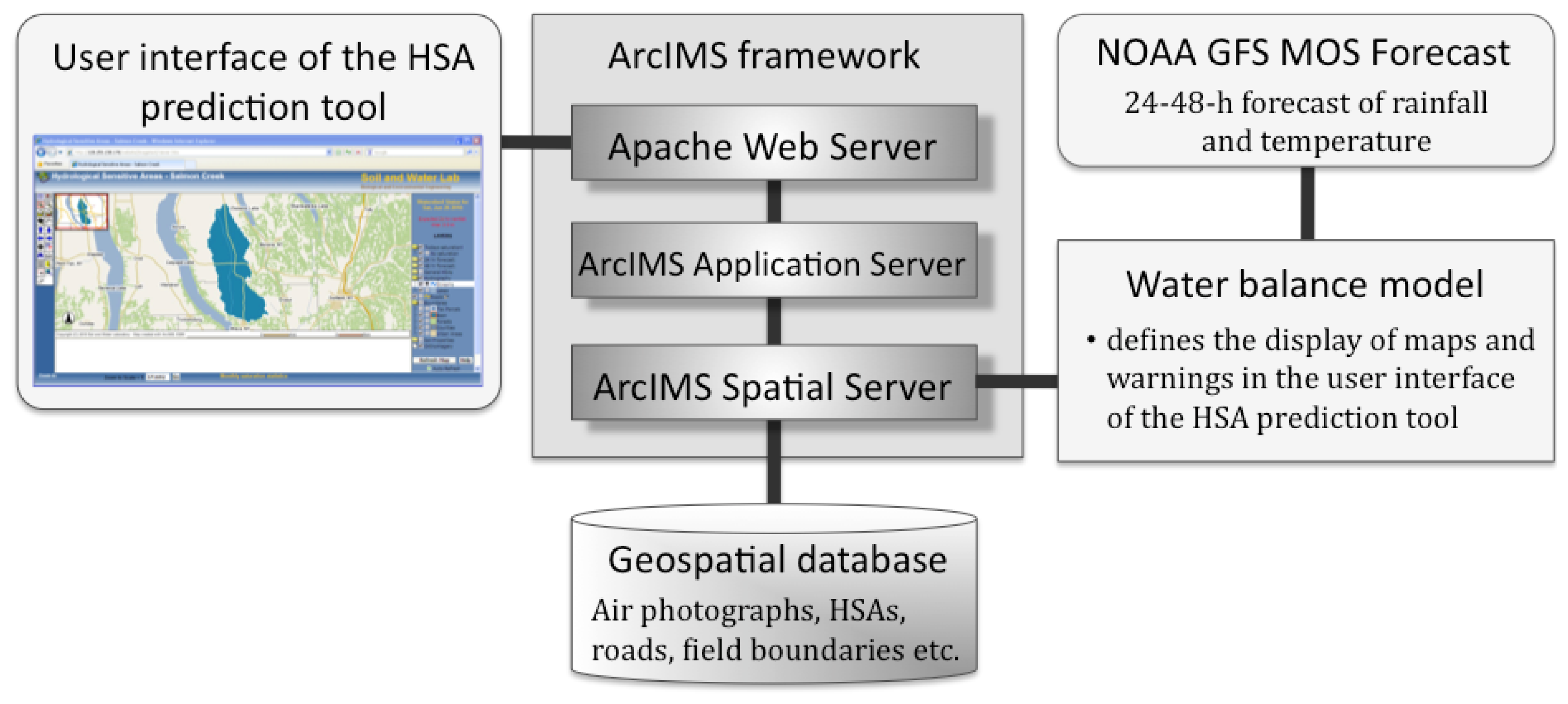
2.1. The Framework of the HSA Prediction Tool

The HSA prediction tool was developed using ArcIMS 9.2 software (ESRI Inc., Redlands, CA, USA). ArcIMS was chosen as a platform to provide a user-friendly, internet accessible interface that does not require the user to install software on a local computer. The HSA prediction tool integrates a pre-calibrated (watershed-specific) water balance model that represents the integration of several standard hydrologic models and four decades of VSA hydrology research [14,16,17,22,34,49]. This VSA water balance model is a semi-distributed model that is based on the Thornthwaite-Mather soil water budget model [51] and predicts the location of VSAs and the amount of runoff contributed from them during storm events. In the HSA prediction tool the VSA water balance model is used to make quantitative predictions of present day and future runoff amounts and HSA extents in space and time through the use of 24–48 h temperature and precipitation forecasts from the Global Forecast System Model Output Statistic (GFS MOS) ensemble data. The VSA model is run with a Python script that also handles the real-time and forecasted meteorological data input to the VSA water balance model and the output of predicted HSA maps on the webpage of the HSA prediction tool. Figure 1 provides an overview of the different components of the HSA prediction tool and their integration into the ArcIMS framework. One advantage of using the ArcIMS framework is that the web-based interface isolates all the water-balance-model-related complexity, such as the model calibration, from the user, thus, facilitating use by a wide audience. Currently, water managers, producers and farmers who retrieve information about current and predicted rainfall-runoff conditions and HSA locations from the web-interface of the HSA prediction tool do not have access to the HSA prediction tool components such as the VSA water balance model. In order to implement or calibrate the VSA water balance model for other watersheds in the region full access to the framework (e.g., the web server) is required, which could be given to state agents or extension specialists. The HSA prediction tool can be easily set up for other watersheds in a simple copy-and-paste process of the ArcIMS framework, requiring only updates of the geospatial data to be displayed and the watershed-specific calibration of the water balance model (see Section 2.2.3).
Figure 1. Integrated system components of the hydrologically sensitive area (HSA) prediction tool.
Water 05 00917 g001

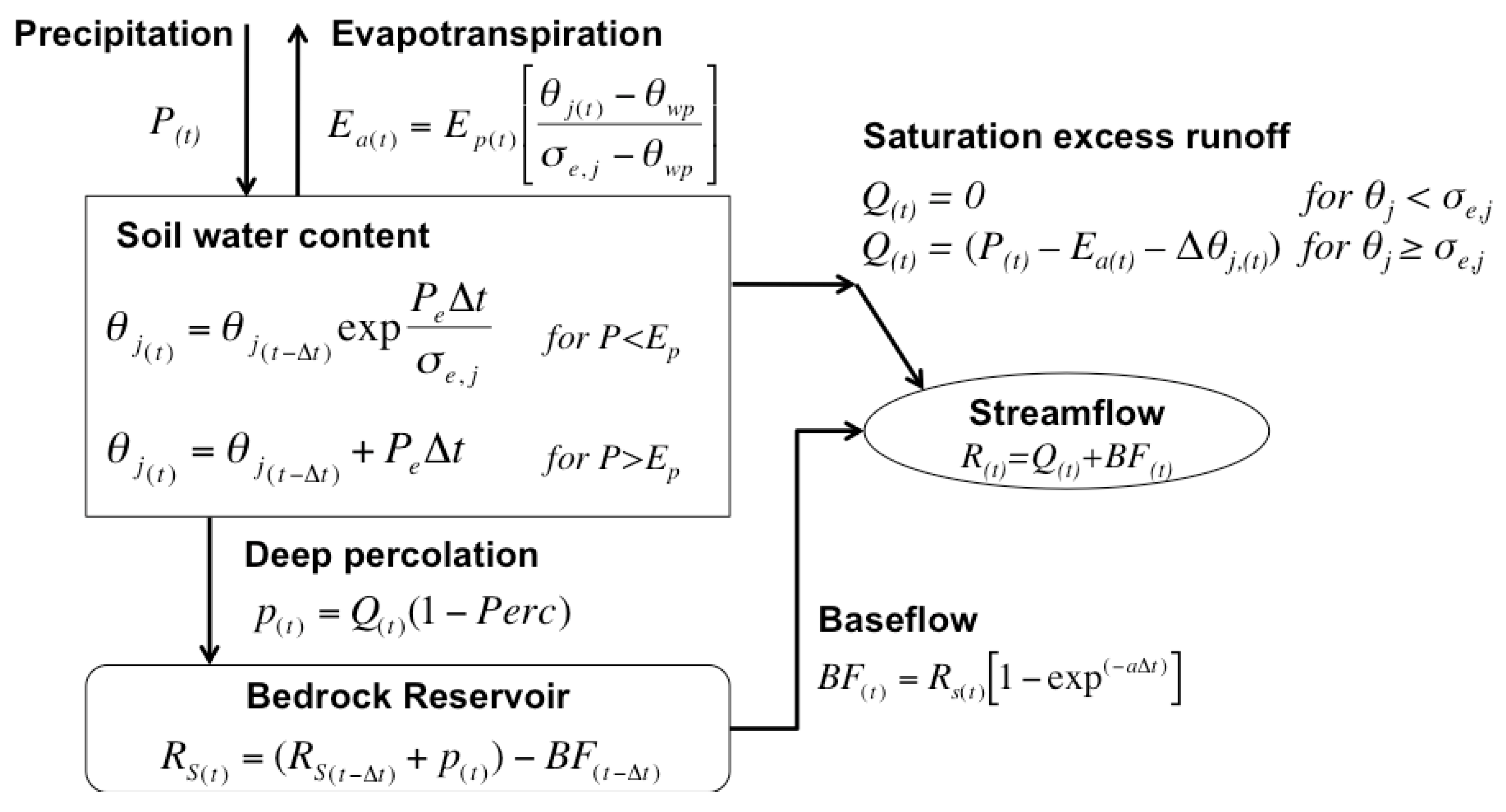
2.2. The Semi-Distributed VSA Water Balance Model

Hydrologically sensitive areas displayed by the HSA prediction tool are predicted with a pre-calibrated (i.e., watershed specific), semi-distributed water balance model that is invisible to the user. This VSA water balance model is based on the Thornthwaite-Mather soil water budget model [51] for which Steenhuis et al. [49] developed an adaptation to VSA hydrologic conditions using the Soil Conservation Service-Curve Number (SCS-CN). The model predicts the location of VSAs and the amount of runoff contributed from them during storm events. Thus, it is designed for applications in watersheds dominated by saturation-excess overland flow. The model has been developed and tested in various VSA hydrology-dominated watersheds [18,19,24,25,26]. The model operates on a daily time step and uses readily available inputs such as daily precipitation, minimum and maximum temperature, as well as topography (digital elevation model) and soil characteristics (soil depth and saturated hydraulic conductivity) to distribute and locate saturated areas in the landscape with the soil topographic index [10,18,25,35,52,53,54,55]. The soil topographic index provides a spatial means to determine relative propensities for saturation within watersheds where water distribution is strongly driven by topography and soils properties, such as depth-to and type-of flow restricting sub-soil layers (i.e., fragipan). The water balance model integrates several concepts presented in the following sub-sections. For a more detailed description of the model and its modifications see [19,24,25].

2.2.1. The VSA Hydrology Concept Based on the Soil Conservation Service (SCS)-Curve Number (CN)

For watersheds dominated by saturation excess overland flow, Steenhuis et al. [49] showed that the fraction of the watershed that produces runoff (Af) can be estimated from the ratio of the change runoff depth (ΔQ) to change in precipitation depth (ΔP). The SCS curve number equation is often used to predict storm runoff from a watershed. The form typically used is the following (USDA-SCS, 1972):
Water 05 00917 i002
where P (mm) is the total precipitation (and snowmelt), Ia (mm) is the initial abstraction, S (mm) is the depth of the watershed-wide storage of water in the soil profile, Pe (mm) is the depth of effective precipitation after runoff begins (PIa). The initial abstraction is the amount of water required to initiate runoff or in terms of VSA hydrology, Ia (mm) is the soil water deficit to be satisfied before complete effective saturation of the soil profile (e.g., water table within 10 cm of surface, [14]) is reached, after which additional rainfall becomes surface runoff. However, in the standard SCS-CN procedure Ia is generally taken as 0.2S, which implies that the fraction of rainfall retained by the watershed prior to the beginning of runoff is storm invariant. To consider variations in the watershed’s soil moisture balance and their impact on storm runoff generation, a modification developed by Dahlke et al. [25] was implemented that allows estimation of Pe based on the actual soil water deficit in the watershed prior to the storm. Specifically, Pe is calculated as the amount of precipitation and snowmelt on the day of the event minus the sum of the actual evapotranspiration (Ea) (mm) of all days (t) since the last rainfall event:
Water 05 00917 i003
If rainfall or snowmelt occurs on the previous day, the water deficit is calculated differently, because the watershed is not in equilibrium. In this case we subtract the previous day’s saturation excess runoff and the previous and current day’s evapotranspiration from the precipitation of the previous and current day.
Water 05 00917 i004

2.2.2. Model Discretization and Variable Source Area Prediction

As shown by Steenhuis et al. [49], the saturated fraction (Af) of the watershed contributing runoff can be estimated by integrating the SCS-CN runoff equation [56] [Equation (1)] with respect to the effective precipitation, Pe:
Water 05 00917 i005
where S (mm) is the depth of the watershed-wide storage in the soil profile, and Pe (mm) is the amount of rainfall that effectively generates runoff, or the total storm precipitation minus the moisture-deficit-dependent initial abstraction (Ia). When Pe = 0, Af equals zero and when Pe approaches infinity the contributing area, Af, equals 1.
In order to capture the spatiotemporal differences in the watershed-wide storage the water balance model considers spatial differences in the fractional contributing area for a storm event by estimating the maximum effective (local) available soil moisture storage, σe,j, for a given area based on the watershed-wide storage, S [26]:
Water 05 00917 i006
where σe,j is the maximum effective available soil water storage of a defined fraction j of the watershed, S is the depth of the watershed-wide storage, and As,j (%) is the percent of the watershed area that has a local effective soil water storage less than or equal to σe,j. In accordance with [26], areas with a high propensity of generating runoff are characterized by a small maximum effective storage, (σe,j), while areas of the watershed that are dryer have a greater maximum effective storage. At any time, the available water content in each wetness class varies between zero (wilting point) and σe,j.
In humid regions where water distribution in the landscape is strongly driven by topography, the soil topographic index, STI, derived from a digital elevation model (DEM) [53] has been shown to be a good predictor for locations of fractional runoff contributing areas, Af, within watersheds [25,35,54,55]. The STI is calculated based on the following equation:
Water 05 00917 i007
where a is the upslope contributing area (m2 per unit contour length), β is the local surface topographic slope (radians), D is the local soil depth (m), and Ks is the saturated hydraulic conductivity (m·day−1). The STI provides a means to locate areas with differing probabilities or risks of generating runoff within a watershed [22,35]. In order to translate saturated fractional area, Af, predictions from the water balance model into HSA risk maps the watershed is divided into 10 wetness classes of equal area using the STI. Wetness class 1 is associated with the largest 10% of STI values that cover the watershed area (Af-values of >0 to 0.1). Wetness class 1 denotes areas that are most prone to saturation and have the smallest maximum effective storage (σe,1). Wetness class 2 is associated with the next wettest 10% of the watershed (Af-values of 0.1–0.2), the second highest STI values and the second smallest maximum effective storage (σe,2), etc. These wetness classes reflect that different areas of the watershed begin contributing runoff at different times depending on the amount of rainfall the watershed receives and its relative storage. A spatial map of each wetness class is subsequently displayed on the web-interface of the HSA prediction tool, indicating potential runoff and pollutant source areas (also called HSA risk maps), if the water balance model predicts saturation-excess runoff generation for some parts of a watershed based on current and forecasted weather conditions. The spatial resolution of the wetness classes and HSA risk maps displayed by the HSA prediction tool is determined by the spatial resolution of the DEM used to calculate the STI.

2.2.3. Model Input, Output and Calibration Parameters

The water balance model estimates the soil water content, θj, in the topmost soil layer of each wetness class based on the Thornthwaite-Mather equation [51], the saturation excess runoff, Q, at the watershed outlet and the percentage of the watershed, Af, that is saturated and generating runoff during storm events using precipitation (and snowmelt), P (mm·day−1), and potential evapotranspiration, Ep (mm·day−1), as input parameters (Figure 2). Note, we use the term saturated areas and runoff generating areas interchangeably recognizing that the soil may not need to be fully saturated to generate storm runoff as shown by [14].
Figure 2. Conceptual diagram of the water balance model, which estimates the soil water content θj in each wetness class j and the saturation excess runoff, Q, at the watershed outlet using precipitation, P, and potential evapotranspiration Ep in each time step (t). Ea is the actual evapotranspiration, θfc and θwp are the soil water content at field capacity and at wilting point respectively, σe,j is the maximum effective soil storage of wetness class j, Pe is the effective precipitation (Pe =PEp), Perc is a percolation coefficient determining the amount of water, p, percolating to the bedrock reservoir, Rs and a is a recession coefficient controlling the rate at which baseflow, BF, is contributed from the bedrock reservoir to the watershed’s streamflow, R.
Water 05 00917 g002
Overall, the model requires calibration of only four parameters: S, Perc, and α for the summer and winter period. In the water balance model the depth of the watershed-wide soil water storage, S, [Equation (1)] becomes a calibration parameter that can be derived directly from baseflow-separated streamflow data [18,19,25] and not on the basis of averaging the curve numbers of the various land uses in the watershed [57]. During wet periods, when rainfall exceeds evapotranspiration or the moisture content exceeds field capacity, θj is determined from the previous day’s moisture plus the effective precipitation (PEp). During dry periods when evapotranspiration exceeds rainfall (i.e., P < Ep), the moisture content of the soil decreases by the actual daily evapotranspiration, Ea (mm). Ea is assumed to decrease linearly from the potential evapotranspiration rate when the soil is at (or above) field capacity, θfc, to zero at the wilting point, θwp. Ep could be calculated by a number of approaches, e.g., Priestley-Taylor [58], but here we simply used a sinusoidal function calibrated to observed Ep data. Since watersheds in the northeast U.S. show large runoff fractions resulting from snowmelt a snow energy balance model by Walter et al. [59] was incorporated into the water balance model. This means that measured or predicted precipitation is first processed in the snow energy balance, which estimates melt rates based on minimum and maximum temperature only, before being evenly distributed over the entire watershed. Any water added that exceeds the local soil storage of each wetness class is partitioned between saturation excess runoff Q (mm·day−1) and recharge to a bedrock reservoir using a percolation coefficient, Perc (mm·day−1). Streamflow, R (mm·day−1), is computed for each time step by adding the saturation excess runoff, Q, to the baseflow; the latter is calculated as a fraction of the bedrock reservoir using a calibrated baseflow recession coefficient, α (day−1), [19], which can have different values for the dry summer and wet winter period.
The water balance model uses a time series of daily measured temperature and precipitation data to simulate soil moisture patterns across a watershed until the present day. In addition, the model uses NOAA GFS MOS weather ensemble predictions, released on the present day for the next 192 h, to simulate soil moisture and associated storm runoff for “today”, and the following 24 h (“tomorrow”) and 48 h (“the day after tomorrow”). Based on the estimation of the saturated fractional watershed area for “today” (Af,t), “tomorrow” (Af,24 h) and the “day after tomorrow” (Af,48 h), the HSA prediction tool presents this information as HSA risk maps to the user in the form of red areas on top of georeferenced aerial photographs. To simplify the presentation, the calculated Af-values are categorized into 10 incremental classes (e.g., 10%, 20%, 30%, etc.) identical to the wetness classes described in Section 2.2.2.

2.3. Hydrologic Forecasting

For the 24 and 48 h forecasts of the saturated fractional watershed area, the water balance model is using forecasted temperature and precipitation estimates of the Model Output Statistics (MOS) [60] generated with the Global Forecast System (GFS). GFS forecasts are released through the National Weather Service via online providers such as NOAA. The messages contain forecasts/projections of a set of meteorological parameters such as maximum daytime and minimum nighttime temperature, wind speed, probability and quantity of precipitation, snow, and mean total sky cover that are valid over at least a 12 h period. The GFS MOS guidance data used in the HSA prediction tool result from the Medium Range Forecast (MRF) run of the NCEP’s (National Centers for Environmental Prediction) Global Spectral Model [61], which has been referred to as the Global Forecast System (GFS) model since 2002 [62]. The medium range MOS guidance provides projections of 24 to 192 h for most weather elements either as graphical maps or as alphanumeric messages. The alphanumeric message containing medium range MOS GFS projections is published twice a day at 0000 and 1200 UTC (Universal Time Coordinate) for approximately 1693 sites, mostly airport locations, within the contiguous United States and Alaska [62].
From the alphanumeric message three parameters, the 24 h quantitative precipitation (Q24), the 24 h probability of precipitation (P24), and the maximum daytime and minimum nighttime temperature (X/N) data are used in the hydrologic forecast module of the HSA prediction tool. The MOS guidance provides exact (i.e., unit true) projections for the minimum and maximum temperature; however, precipitation amounts in the 192 h projection are only given in categorical form in the alphanumerical message (Table 1). We decided to use the maximum value of the predicted precipitation category as input to the water balance model on grounds of estimating the “worst case scenario” HSA extents for a predicted storm event. In the HSA prediction tool the temperature and precipitation projections from the GFS MOS ensembles are automatically retrieved from the alphanumeric message via a direct URL link using a python script. This python script runs on a daily basis at 4:00 AM local time and adds the forecasted temperature and precipitation data to a time series data file used as input for the VSA water balance model. At the same time the temperature and precipitation records of the previous day, which exist from the GFS MOS query made on the previous day, are replaced with measured data from a climate station located within the watershed, to which the VSA water balance model is calibrated. If the real-time climate station data has missing data points, then the GFS MOS data are used to fill existing gaps.
The probability of precipitation (P24) is extracted daily from the alphanumerical message and disseminated to the user in a separate browser window. A summary of the expected hydrological conditions in the watershed and the likelihood of occurrence of a storm event within the next 24 h and 48 h are provided in a short text message. The P24 forecast provides an estimate of the probability of precipitation (PoP) for a projected 24 h period. Values range from 0 to 100%. Both PoP projections for the next 24 h and 48 h are provided to the user in the summary of expected hydrologic conditions (Figure 3).
Table 1. Categories of the quantitative precipitation forecast provided with in the Global Forecast System (GFS) alphanumerical message and its usage in the water balance model.
CategoriesGFS precipitation scale (in.)Precipitation (mm) used in the VSA water balance model
000.0
10.01–0.092.3
20.10–0.246.1
30.25–0.4912.5
40.50–0.9925.2
51.00–1.9950.6
6≥276.2
Figure 3. Daily updated status report showing the forecasted rainfall amounts, the probability of precipitation for each projected 24 h period, and the expected percent area of the watershed that could saturate or generate runoff.
Water 05 00917 g003

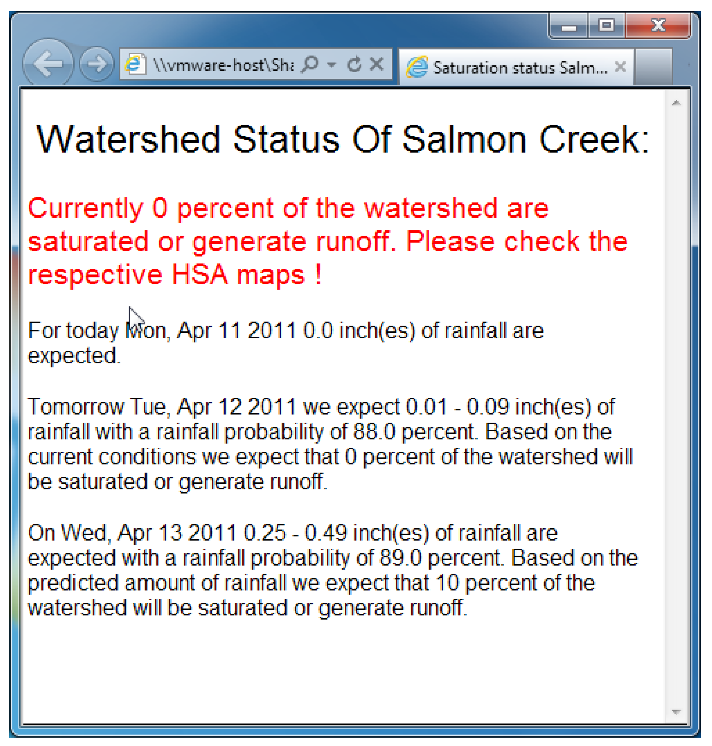
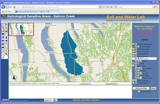
2.4. User Interface of the HSA Prediction Tool

The HSA prediction tool is a map service that is accessible through a web browser. The tool is designed to be used by producers and stakeholders on a daily basis. The main page for the watershed used in the presented prototype application [63] is shown in Figure 4, which provides standard interface features such as a large map of the area of interest, an overview map, a navigation tool bar, and features that allow information retrieval on the displayed geographical data (e.g., query, feature identification). Information regarding the current (“Today’s forecast”) and forecasted ( “24 h forecast” and “48 h forecast”) hydrologic conditions and saturated area extents are displayed in the upper part of the right layer frame (Figure 5). Below these three layers the tool provides a list of watershed-specific geographical data containing the potential HSA risk maps, infrastructure (i.e., hydrography, roads), administrative boundaries and soils properties. The user can query information contained in these geospatial data sets for a specific site using the query tool. The query results are displayed at the bottom of the window (Figure 5). Above the layer list the user is presented with a short summary of the hydrological conditions (e.g., “Expected 24 h rainfall: max. 0.0 in.”) (Figure 4) and a link (highlighted in yellow) that opens a separate “status report” window summarizing the expected rainfall amounts, rainfall probabilities and the estimated percentage of the watershed that is predicted to saturate or generate runoff within the next 24–48 h (Figure 3); note, English units are displayed because most users are less familiar with SI units.
Figure 4. Start page and user interface of the HSA prediction tool.
Water 05 00917 g004
Figure 5. User interface of the HSA prediction tool. Red areas show HSA predicted with the semi-distributed water balance model. A daily update of forecasted weather conditions and HSA dynamics in Salmon Creek watershed is given in the top, right frame.
Water 05 00917 g005

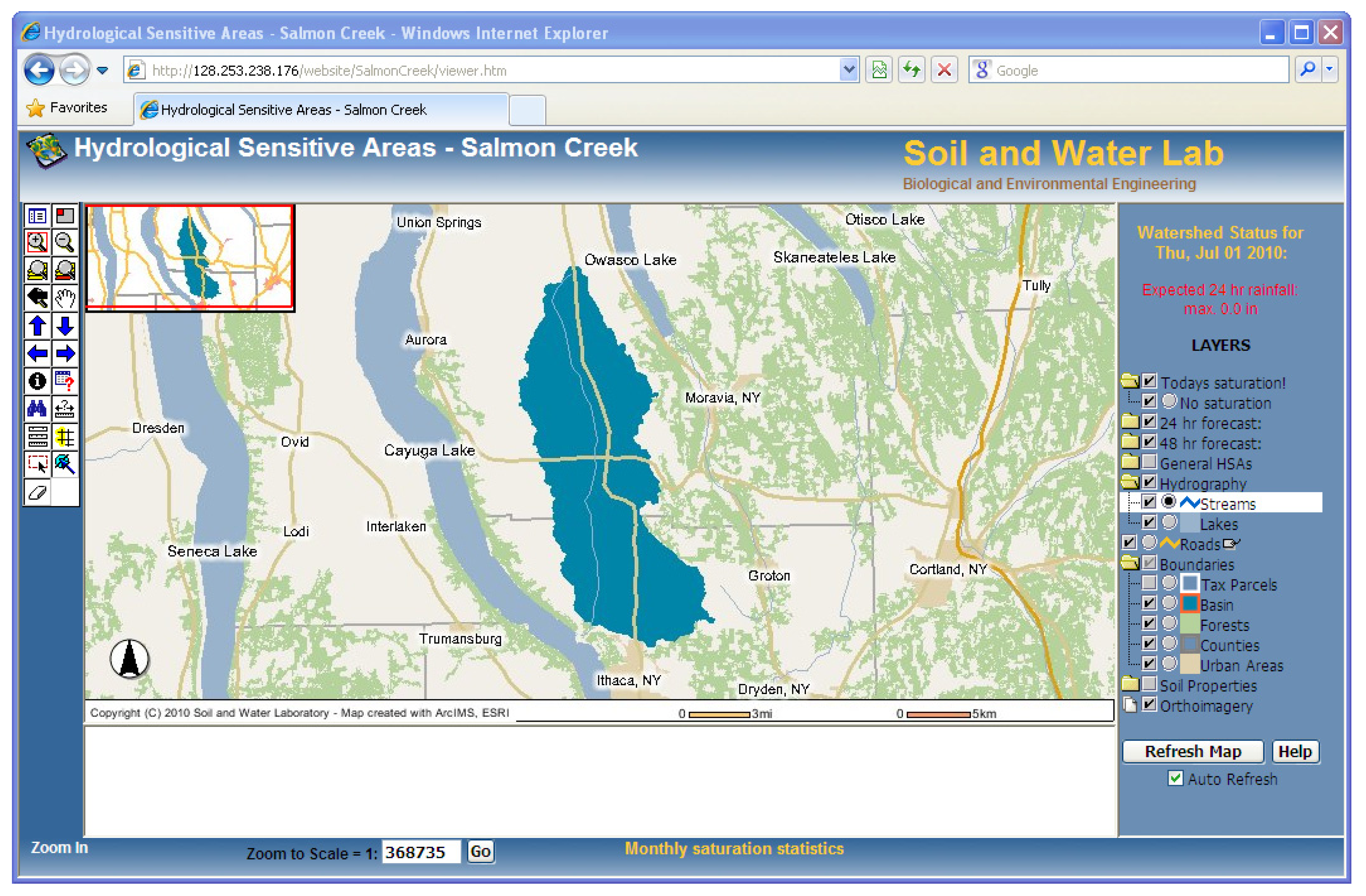
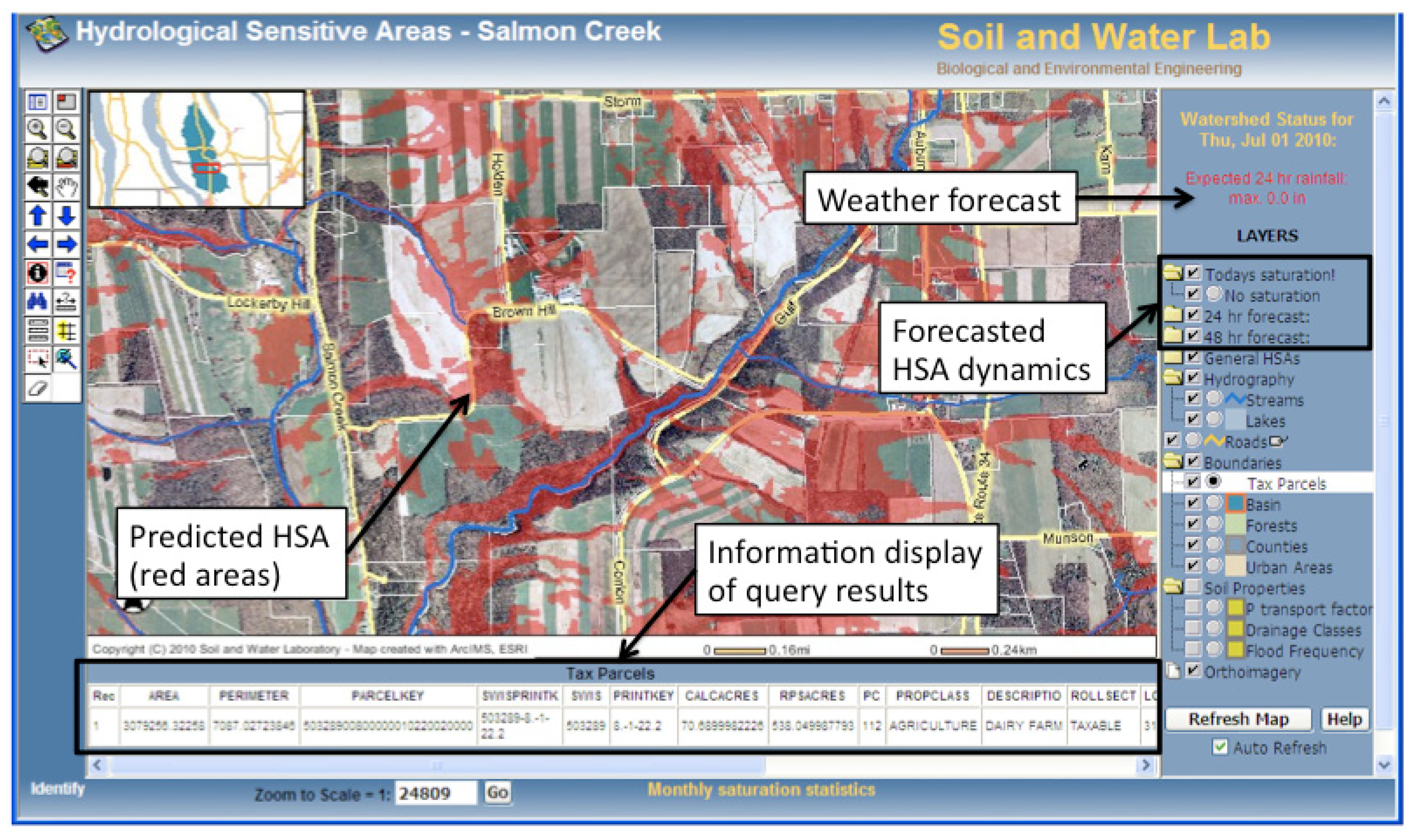
2.4.1. Graphical Output of Predicted HSA Risk Maps

Based on the water balance model output, the top three layers listed in the right-hand-side frame display maps of the predicted percentage of the watershed that is currently or expected to be saturated within the next 24–48 h. These areas are highlighted in red and ultimately visible to the user when the user has zoomed into an area of interest with a scale of greater than 1:100,000 (Figure 5). If no saturated areas are predicted by the water balance model, the message “no saturation!” is displayed in the right-hand-side frame and the red HSA maps are not displayed in the main map. For more general risk information, the user can also view each potential 10% (see Section 2.2.2) runoff risk class (e.g., 90%) in the watershed, which is provided by separate “General HSA” layers in the layer frame of the HSA prediction tool (Figure 5).

2.4.2. Geospatial Data

The HSA prediction tool uses a set of various geospatial data sets to inform and educate planners and producers about the current and forecasted risk of occurrence of runoff source areas. For the developed prototype of the HSA prediction tool, the geospatial database is comprised of raster and vector data sets (i.e., shapefiles) that help the user locate their area of interest (e.g., a specific farm) and retrieve property and field boundary information for orientation (e.g., via tax parcel code). The displayed data sets include the local stream network, lakes, roads, urban areas, county and tax parcel boundaries, land cover information as well as aerial photographs of the watershed and surrounding areas. In addition, the web-based tool displays soil classification information from the Soil Survey Geographic (SSURGO) database [64], in particular the flood frequency and soil drainage class. These geospatial data sets are provided to assist producers and planners in the calculation of the NYS P-Index and the estimation of the nutrient loss risk from specific fields. The database further contains the watershed-specific HSA risk maps, which are derived from a 10 m USGS digital elevation model (DEM) using the method described in Section 2.2.2.

3. Application of the HSA Prediction Tool: Proof of Concept
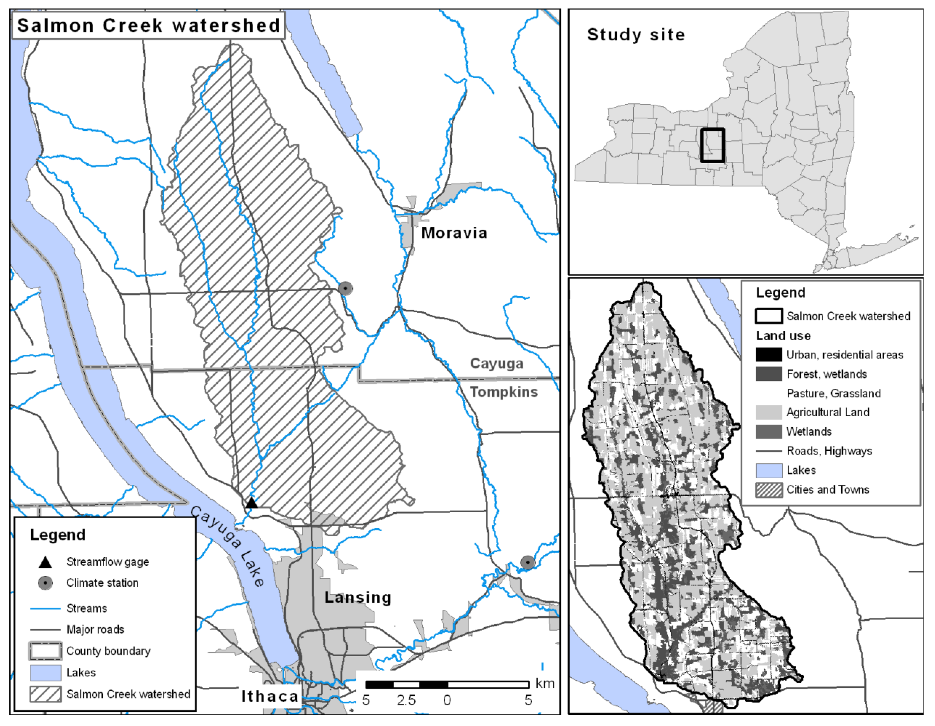
As a proof of concept, a prototype HSA prediction tool was developed for the 230 km2 Salmon Creek watershed (Figure 6), located north of Ithaca in NYS. The watershed is located in the glaciated Allegheny Plateau physiographic region. The annual average temperature is 8 °C; average annual precipitation is 93 cm, with 173 cm of snowfall annually. Land use consists of 70% agricultural land, 28% mixed forest, and the remaining 2% is residential, commercial, and urban (Figure 6). Soils are generally 200 cm deep, with well to somewhat poorly drained silt loams and gravelly silt loams [64]. Elevations range from 320 to 378 m. The watershed exhibits typical HSA type hydrology due to the shallow highly permeable soils overlaying a dense fragipan at a shallow depth [29].
Figure 6. Location and characteristics of Salmon Creek watershed.
Water 05 00917 g006

3.1. Input Data

3.1.1. Geospatial Database

A geospatial database was developed for the Salmon Creek watershed (76.54° W, 42.54° N) that is comprised of image raster and vector data required for the development of the watershed-specific HSA prediction tool. Table 2 provides a summary of the geospatial data sets and sources used in the Salmon Creek HSA prediction tool. All data displayed in the geographic area of Salmon Creek are projected in UTM coordinates, Zone 18 with the North American Datum 1983.
Table 2. Multisource geospatial and hydro-meteorological database developed for the HSA prediction tool.
DataResolution/ScaleSourceDescription
Air photographs2 mNY State GIS Clearinghouse [65]Natural color image. Cayuga County 2007, Tompkins County 2006.
DEM10 mNYS DEC, USGS [66]Elevation, slope, flow direction, flow accumulation, HSAs
Forest30 mMulti-Resolution Land Characteristics (MRLC) Consortium [67]Land Use, Land Cover data set, 2001
Lakes1:2,000,000National Atlas, New York State [66]Lakes and surface water bodies
Roads1:100,000U.S. Census Bureau [66]
Soils1:15,840 (Cayuga County)
1:20,000 (Tompkins County)
SSURGO (USDA-NRCS Soil Data Mart) [64]Soil depth, saturated hydraulic conductivity, drainage class, flood frequency
Streams1:100,000U.S. Census Bureau [66]Hydrography
Tax Parcels1:10,000Tompkins County and Cayuga County Clerkʼs Office [66]Municipal Tax Parcels (year 2000)
Urban areas1:100,000U.S. Census Bureau [66]Urbanized areas and municipalities
Meteorological data Northeastern Regional Climate Center [68]Daily minimum and maximum temperature and total daily precipitation
Streamflow data U.S. Geological Survey [69]Daily streamflow data
GFS MOS forecast data NOAA National Weather Service [70]Extended range GFS-Based Model Output Statistics (MOS)

3.1.2. Weather Data

Precipitation and temperature data for Salmon Creek were downloaded from two Northeast Regional Climate Center (NRCC) weather stations located in Locke, (42.67° N, 76.47° W, station ID 304836) and Freeville (42.52° N, 76.33° W, station ID 303050), NY (Figure 6). For the 24–48 h forecast of HSA dynamics in Salmon Creek temperature and precipitation projections from the closest GFS MOS site, the Ithaca airport station (station ID KITH) (42.48° N, 76.47° W) located approximately 10 km south of the Salmon Creek stream gage, is used. Minimum and maximum potential evaporation varied between 0 and 4 mm [71]. Daily streamflow data were available for the period 22 July 2006 until 31 December 2009 measured by the U.S. Geological Survey (USGS, station ID 0423401815) at the outlet of Salmon Creek watershed in Ludlowville, NY (42.55° N, 76.53° W).

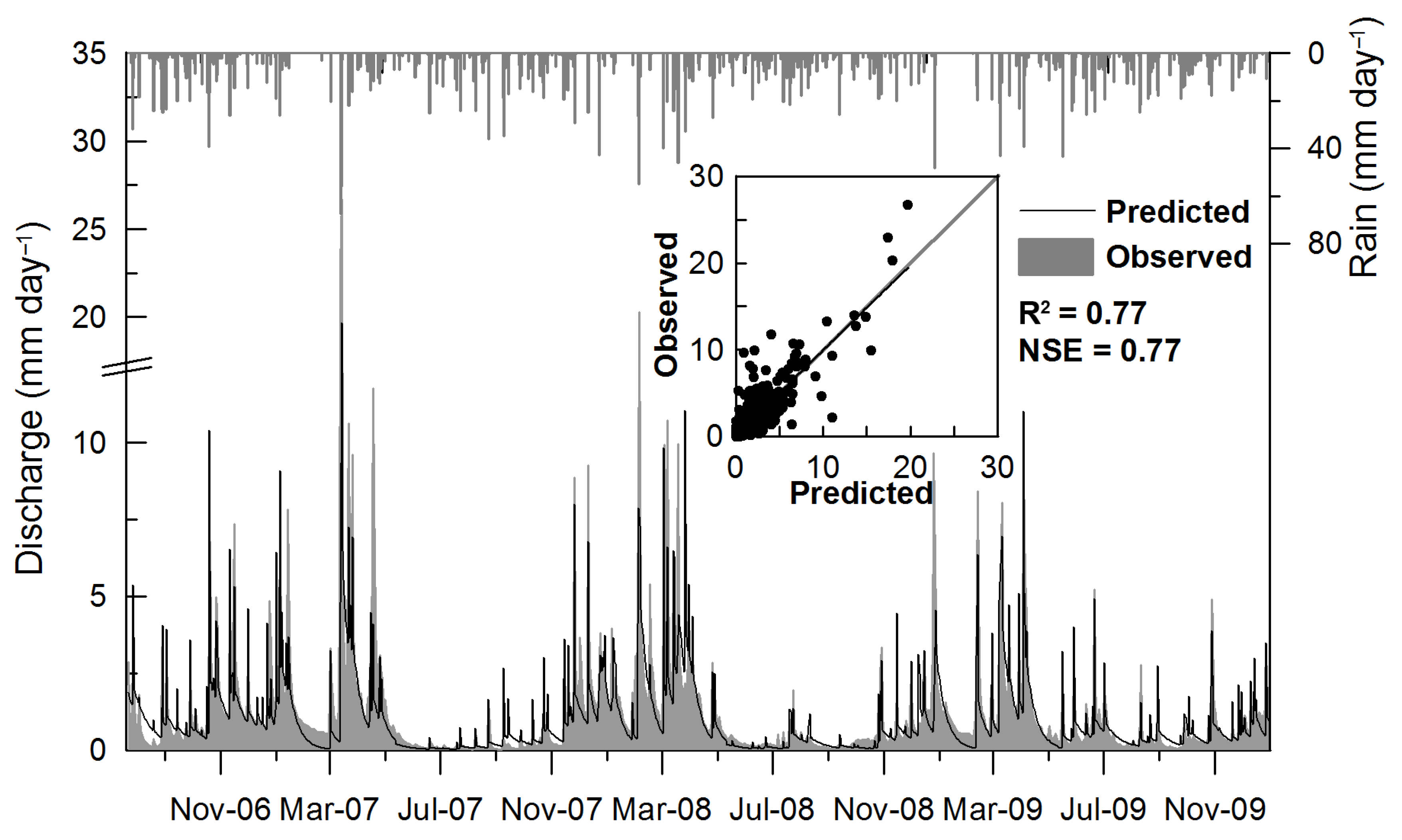
3.2. VSA Water Balance Model Calibration and Validation

The water balance model requires calibration of four parameters, the effective watershed storage, S, the baseflow recession coefficients for summer and winter, αs and αw, and the percolation coefficient, Perc. The overall effective storage of the watershed was calibrated to baseflow-separated runoff (S = 20 cm). Based on S the maximum effective soil moisture storage, σe,j, for each wetness class was determined using Equation (5). The baseflow recession coefficients for the summer (May–October) and winter season (November–April) were calibrated from baseflow separated streamflow [17] and equaled αs = 0.06 (day−1) for summer and αw = 0.09 (day−1) for winter. The percolation fraction was calibrated to Perc = 0.74 (mm·day−1) by maximizing the Nash-Sutcliffe efficiency over the calibration period using a nonlinear optimization algorithm (e.g., Microsoft Excel Solver). The model was calibrated using precipitation from Locke, temperature from Freeville and streamflow data measured at the outlet of Salmon Creek watershed for the period 22 July 2006 to 21 July 2008. Streamflow data observed for the period 22 July 2008 until 31 December 2009 were used to validate the model performance.
The coefficient of determination, R2, for the linear regression between daily measured and modeled streamflow for the calibration period is R2 = 0.76 and Nash-Sutcliffe efficiency (E) [72] is E = 0.76 and, for the validation period, R2 = 0.79 and E = 0.78. Table 3 gives summary statistics for measured and modeled average streamflow amounts for each year of the entire modeling period. Daily streamflow was generally well predicted during the entire modeling period (Figure 7). Streamflow was more accurately predicted during the wet winter months when the majority of total and dissolved P is exported from watersheds in the humid northeastern U.S. [73,74,75,76] than during the generally drier summer months. Major storm events were particularly well predicted during 2007 and 2009 but slightly under-predicted in 2008. Summer storm runoff was generally over-predicted, likely because catchment connectivity and runoff potential during the drier summer months is reduced and not sufficiently represented by the simple approach of a watershed-wide storage parameter S (Figure 7).
Figure 7. Precipitation (bars) and daily streamflow predicted by the water balance model plotted against the measured streamflow at the catchment outlet of Salmon Creek for the time period 22 July 2006–31 December 2009. The inset shows the linear 1:1 relationship. The coefficient of determination (R2) and Nash-Sutcliffe efficiency (E) are calculated based on the entire modeling period. Table 3 summarizes uncertainty statistics for the calibration and validation period.
Water 05 00917 g007
Table 3. Summary of measured and modeled, annual and seasonal streamflow statistics and goodness-of-fit measures for Salmon Creek watershed. The calibration and validation periods range from 22 July 2006–21 July 2008 and 22 July 2008–31 December 2009, respectively.
PeriodModeledMeasuredGoodness of fit
Minimum (mm·day−1)Mean (mm·day−1)Maximum (mm·day−1)Minimum (mm·day−1)Mean (mm·day−1)Maximum (mm·day−1)E aR² b
20060.371.4510.410.111.4113.250.740.74
20070.021.0921.390.021.3026.710.800.82
20080.041.1217.900.041.2020.300.680.71
20090.060.9913.740.050.9612.720.820.83
Calibration period0.371.4510.410.111.4113.250.760.76
Validation period0.040.8714.850.040.8813.780.780.79
Entire Period c0.021.1121.390.021.1926.710.770.77
Notes: a Nash-Sutcliffe comparison with measured streamflow; b Coefficient of determination comparison with measured streamflow; c The entire modeling period ranges from 21 July 2006 until 31 December 2009.

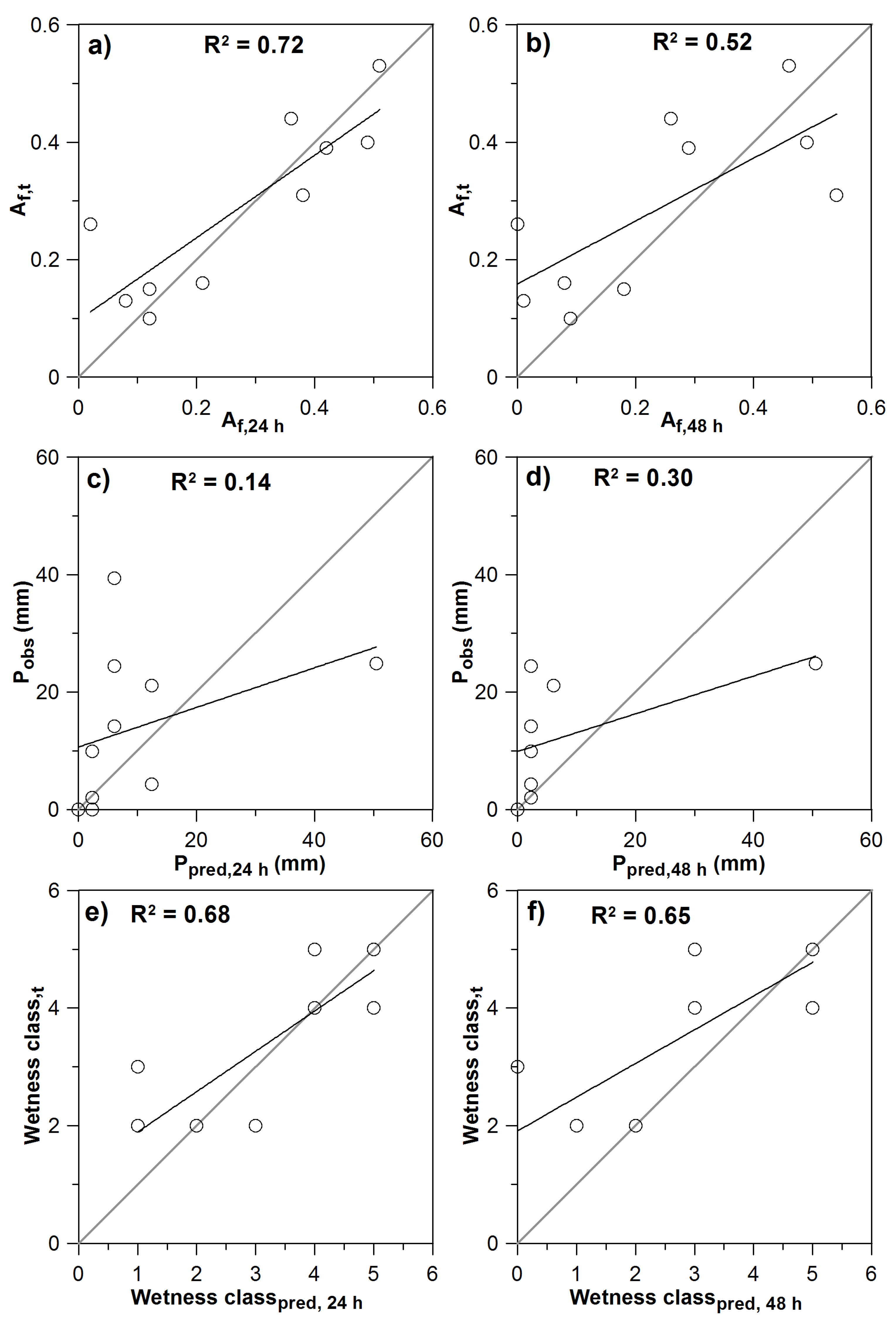
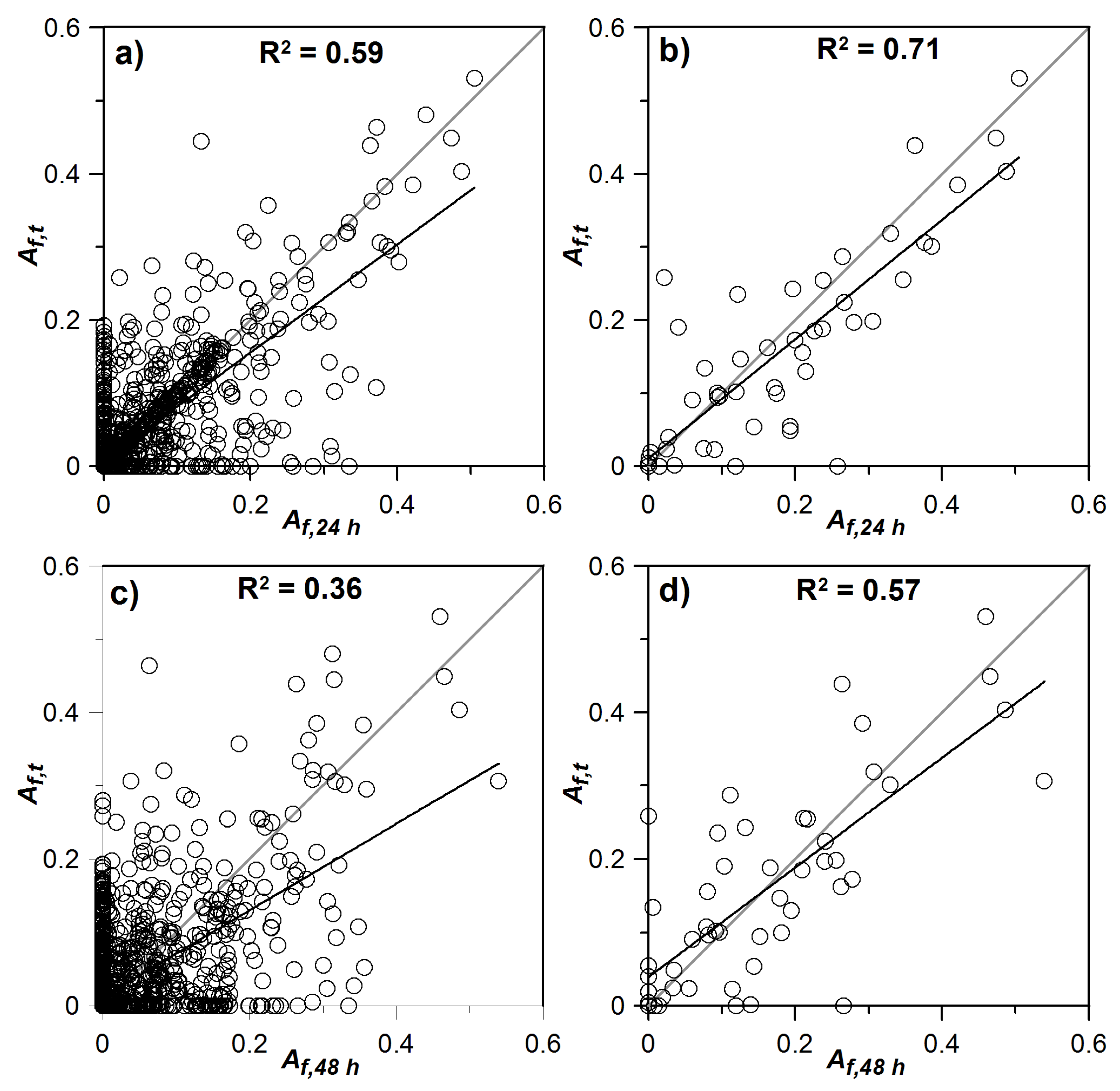
3.3. Accuracy of HSA Predictions for Salmon Creek Watershed

The HSA prediction tool is only of value to watershed managers if runoff and HSA dynamics are correctly and reliably predicted based on the 24–48 h temperature and precipitation projections of the GFS MOS ensemble data. Thus, we compared the fractional saturated areas predicted for the next 24 h and 48 h, denoted by Af,24 h and Af,48 h for the remainder of this article, to Af-values computed based on actual measured temperature and precipitation data from the NRCC climate stations for a given day (denoted by Af,t). In other words, for each day of the modeling period, for example 24 July 2007, we compare the Af-values (Af,t) computed by the water balance model with measured weather data from Locke and Freeville on that day to Af-values computed with GFS MOS weather projections released for 24 July 2007 on the previous day (Af,24 h) and the day before the previous day (Af,48 h).
Figure 8 and Table 4 show the results of the statistical comparison for data pairs of Af-values computed with measured weather data to either the 24 h predicted (Af,t vs. Af,24 h) or 48 h predicted Af-values (Af,t vs. Af,48 h). The coefficient of determination, R2, calculated based on all Af-values estimated with the water balance model for the record period (i.e., including days where no saturation was predicted) was R2 = 0.59 for Af,t vs. Af,24 h and R2 = 0.36 for Af,t vs. Af,48 h. Note, we expect diminished agreement with more distant forecasts because weather forecast uncertainty increases with increased time into the future.
Figure 8. Correlation of saturated fractional areas (Af-values) predicted using observed weather data (Af,t) versus Af-values predicted with 24 h (Af,24 h) forecasted (a,b) and 48 h (Af,48 h) forecasted weather data (c,d). Plots (a) and (c) compare Af-values on a daily basis for the entire record period. Plots (b) and (d) show the correlations for storm events with observed discharges greater than 5 mm·day−1. Grey lines indicate the 1:1 relationship and black lines show fits of a simple linear regression.
Water 05 00917 g008
Table 4. Percentage of days where Af-values predicted based on the 24 h (Af,24 h) and 48 h (Af,48 h) weather projections agree with Af-values computed with measured weather data (Af,t) over the record period of 22 July 2006–31 December 2009.
Comparison setsWetness classes
Alln.s.12345678910
Af,t vs. Af,24 h0.810.920.660.540.500.670.671n.a.n.a.n.a.n.a.
Af,t vs. Af,48 h0.700.870.410.240.250.170.671n.a.n.a.n.a.n.a.
Af,24 h vs. Af,48 h0.790.920.540.460.480.540.501n.a.n.a.n.a.n.a.
Notes: n.s. = indicating non saturated areas, n.a. = not available; these wetness classes did not saturate during the study period.
As illustrated in Figure 8a, most of the larger storm events (indicated by large Af-values) plot along the 1:1 line. For days where Af,t did not match Af,24 h, the difference in the computed fraction of the watershed that contributes runoff was on average less than 0.2 or 20% of the watershed area. In contrast, comparison of Af,t vs. Af,48 h (Figure 8c) shows a more scattered picture and rather an over-prediction of Af-values than computed with actual measured data. Nevertheless, most large Af-values plot again along the 1:1 line. In 81% of the days the 24 h forecasted Af-values agree with the Af,t-values; 70% of the 48 h forecasted Af-values matched the computed Af-values based on measured weather data (Table 4).
As summarized in Table 4, the wetness class-based (e.g., wetness class 2 equals Af-values in the range of 0.1–0.2) comparison of Af-values predicted based on the 24 h projections with Af,t-values agreed in more than 50% of the days in all classes and in more than 67% of the days when large storm events occurred resulting in runoff contributions from 40% to 60% (wetness classes 4–6). The percentage of days where Af-values predicted based on the 48 h projections with Af,t-values agreed is lower, indicating that the 48 h precipitation forecast of the GFS MOS projections is, in general, quantitatively less reliable.
When looking at the 10 largest storm events observed during the record period the coefficient of determination for both comparisons is R2 = 0.72 for Af,t vs. Af,24 h and R2 = 0.52 for Af,t vs. Af,48 h respectively (Figure 9). For these storm events the 24 h and 48 h projection-based Af-values differed from Af-values computed based on measured weather data, on average, by 0.08 and 0.2 (8% and 20%), respectively. This indicates that, based on the GFS MOS weather projections, the estimation of HSA extents of potentially large storm events is very accurate despite the differences between forecasted and observed precipitation amounts. Interestingly, regardless of systematically using the highest predicted rainfall depth from the forecasts, there is no bias towards over-predicted runoff generating areas; if anything there is a systematic under-prediction (Figure 9).
Figure 9. Comparison of modeled fractional saturated areas (a,b), predicted vs. observed precipitation (c,d), and modeled wetness classes (e,f) for the 10 largest storm events observed in Salmon Creek watershed between July 2006 and December 2009. Plots (a) and (b) compare Af,t-values computed with the VSA water balance model based on observed weather data versus Af,24 h, and Af,48 h values modeled using 24 h and 48 h GFS MOS projected meteorological data for each event. Pobs, Ppred,24 h and Ppred,48 h are the observed and 24 h, 48 h forecasted total daily precipitation amounts for these events. Plots (e) and (f) compare the wetness class predicted with the VSA water balance model using observed (wetness class,t) and 24 h (wetness class,24 h) and 48 h (wetness class,48 h) forecasted meteorological data.
Water 05 00917 g009

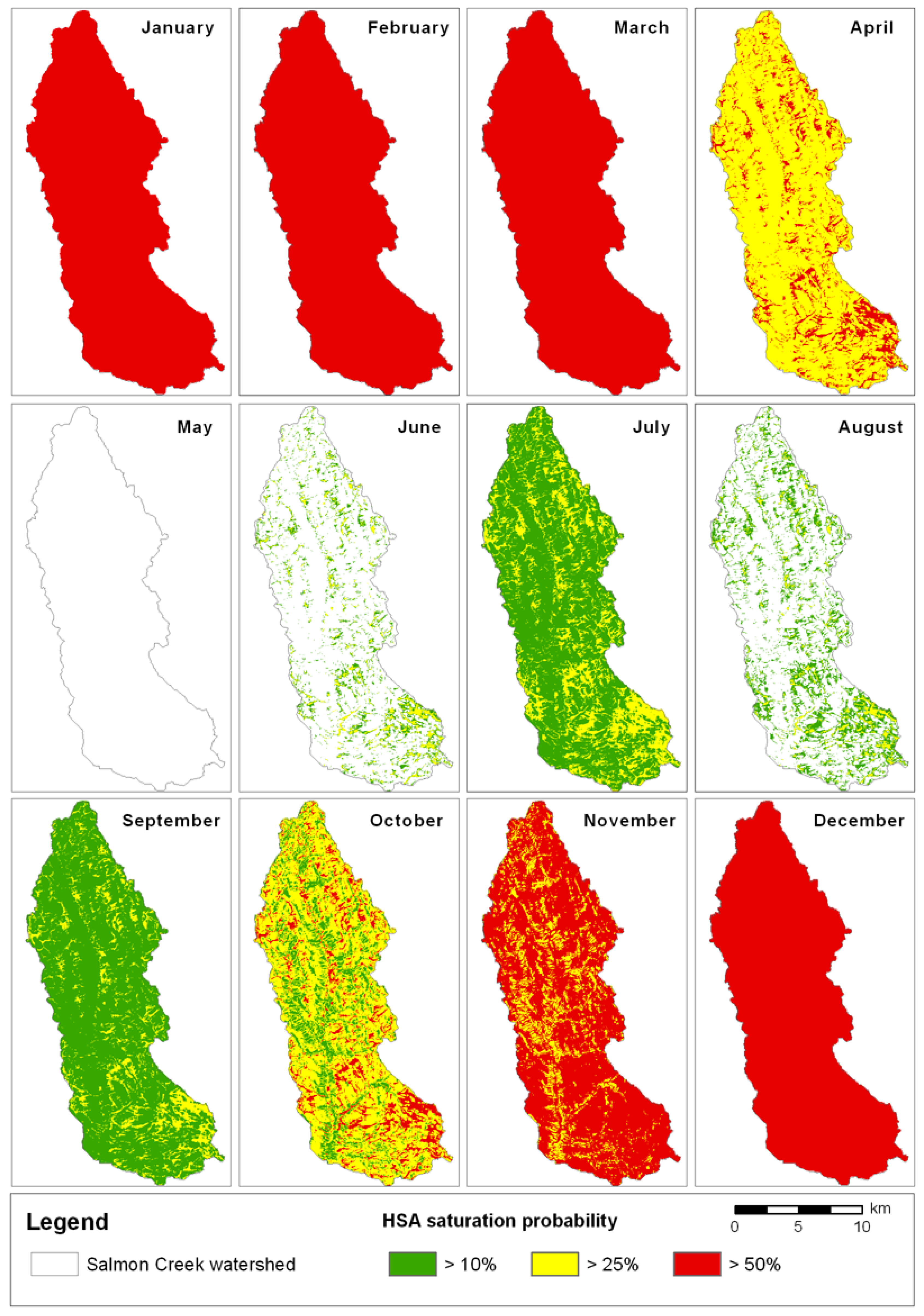
3.4. Predicted Saturation Dynamics

We used the calibrated water balance model to determine long-term monthly saturation dynamics in the Salmon Creek watershed that can be accessed by the user through a hyperlink in the bottom frame of the HSA prediction tool (Figure 4). Average moisture and runoff conditions in Salmon Creek show, in general, a high level of seasonal variability. For each month the probability of saturation can be estimated by taking the ratio of the number of days for which a location within the watershed saturates to the total number of rainfall-days [22,50]. The number of saturation days is predicted with the water balance model; the number of precipitation days is taken from climate stations in Locke and Freeville, NY, USA.
The probability of saturation shown in Table 5 and Figure 10 shows monthly and annual averages estimated over the period July 2006 to December 2009. The months December–March are on average the wettest months of the year where more than 50% of the rainfall and snowmelt events cause the entire watershed to saturate. During October, November, and April 25% of the rainfall events cause the entire watershed area to contribute runoff. Only during the drier summer months (May–August) does the saturation probability decreases below 25%, with May being the driest month and July being the wettest summer month on average (Table 5). The annual probability of saturation statistic indicates that the wettest 10% of the watershed saturates and generates runoff for more than 50% of the rainfall events. The remaining areas of the watershed have the potential to transport nutrients and pollutants to streams, on average, in over 25% of the rainfall events.
Table 5. Probability of saturation for each wetness class and month as predicted with the hydrologic assessment tool in Salmon Creek. Each wetness class represents 10% of the watershed area. Wetness class 1 indicates areas most prone to saturation; wetness class 10 indicates areas least prone to saturation.
Time periodWetness classAverage number of rainfall days
12345678910
January0.940.940.940.940.940.940.940.940.940.947.87
Febuary0.710.710.710.710.710.710.710.710.710.713.50
March0.820.820.820.820.820.820.760.760.760.768.50
April0.620.550.410.410.380.380.380.380.380.3814.50
May0.05 10.00
June0.290.160.03 15.50
July0.360.310.260.240.240.190.190.170.120.1018.08
August0.260.210.140.090.070.020.020.020.020.0214.33
September0.420.280.220.220.220.220.110.110.110.1112.00
October0.610.570.460.410.370.370.350.280.220.2215.33
Novemember0.550.500.500.500.500.500.500.500.480.2313.33
Decemember0.770.730.730.680.680.680.680.680.680.687.33
Annual average0.510.440.380.360.350.340.320.310.290.26140.27
Figure 10. Monthly probability of saturation for Salmon Creek watershed. For each month the factional watershed area is shown that saturates or generates runoff in more than 50% (red areas), 25% (yellow areas) and 10% (green areas) of the rainfall events.
Water 05 00917 g010

4. Management Implications and Conclusions

The HSA prediction tool presented in this paper unites the capacity of a water balance model, optimized for hydrologic predictions in watersheds dominated by saturation-excess overland flow, with 24–48 h projections of weather conditions in a user-friendly, online-available interface. The tool is aimed at identifying and displaying specific parts of the landscape that show a high risk of transport of agricultural chemicals and nutrients to streams via storm runoff. The use of the ArcIMS framework provides an intuitive and user-friendly environment to learn about variable source area hydrology and its implications for NPS pollutant transport. It also enables users to utilize the system without an in-depth knowledge of the individual components and the expertise required to calibrate the water balance model. The prediction of wetness conditions and saturated areas is automatically updated daily based on weather data from nearby NRCC climate stations and GFS MOS projections of temperature and precipitation. The framework is designed such that watershed planners and stakeholders can easily access the tool via a web site that provides basic geographical data for orientation. The HSA prediction tool requires no expertise in VSA hydrology or best management practice (BMP) planning. Thus, it can be easily used by less experienced users.
The implementation of the HSA prediction tool, as presented in this paper, identifies not only the locations of areas prone to saturation or surface runoff, but also determines the risk of NPS pollution by estimating the relative risk of saturation or storm runoff. As shown in Table 5 and Figure 10, the HSA prediction tool provides basic annual and monthly statistics on the probability that a certain part of the watershed is contributing runoff and potentially pollutants during storm events. This information is fundamental to characterize the watershed-specific saturation dynamics of a catchment, which are useful to formulate long-term nutrient management plans. In addition, the daily updated HSA risk maps provide scientifically based means for planners and producers to potentially increase efforts that focus on the day-to-day protection of areas with high transport potential.
The extent of HSAs is modeled based on antecedent moisture conditions and daily rainfall data within a water balance model that allows the usage of the HSA prediction tool for the prediction of HSA dynamics and the scheduling of management activities in the watershed in real-time. The tool can be used to locate fields with low saturation potential that could, potentially receive more liberal manure applications without increasing the risk of NPS pollution. Implementing a tool that provides real-time and 24–48 h HSA predictions will be valuable to watershed managers and stakeholders to, for instance, schedule manure or pesticide applications more precisely in space and time. As such, the tool supports also the optimization of sub-field manure or pesticide applications in response to intra-field variations in short-term moisture conditions and long-term saturation probabilities. Basically, we propose that the targeting of potentially polluting activities away from HSAs constitutes a none-structural, dynamic Control Source BMP. The HSA prediction tool ultimately redefines the HSA-concept such that “areas most likely to generate runoff” no longer refers to the probability based on past weather but, rather, based on current and near-forecast conditions. This is an important paradigm shift in HSAs.
In addition to being a potential component of precision agriculture, the HSA prediction tool has the potential to improve transport-factor estimates in the NYS P-Index, which is used for longer-term nutrient management planning. Specifically, it can provide general geospatial data sets used to calculate the P-Index transport factor (e.g., soil drainage, flood frequency) and, more importantly, provide better and more precise information about the coincidence of fields and HSAs. Recall that the current NYS P-Index identifies high-risk runoff areas based largely on proximity to a watercourse, which is not a reliable proxy of runoff risk [29,35]. Additionally, the current NYS P-Index transport factor is more or less static, restricting the application of manure within a fixed-width 30 m buffer to the stream [33], which has been shown to not effectively abate dissolved phosphorus transport to streams [4,8,9,13]. Recognizing that the location where runoff occurs varies both spatially and temporally and depends on the amount of rainfall and antecedent moisture conditions in the watershed [14,34], the HSA prediction tool provides a means to support the adaptation of variable-width buffers (e.g., derived with the soil topographic index [35]) that capture more realistic runoff generating areas [25,26,35,54] and dissolved nutrient transport via shallow subsurface storm flow [34,77]. Furthermore, the spatial maps provided in the VSA prediction tool support the development of other land management decisions (e.g., riparian buffers) that can also be effective of keeping pollutants from being directly introduced to streams. In addition, the HSA prediction tool provides sub-field information about the month-to-month variability in hydrologic sensitivity for longer-term manure-application scheduling. Thus, using the HSA prediction tool planners and farmers can achieve more flexibility in planning applications of nutrients or pesticides based on the characteristics of the land at larger spatial and temporal scales than they currently use. In the near future we intend to meet with farmers and planners to evaluate the efficiency and applicability of the HSA prediction tool. However, the web-based approach provides unlimited opportunities to update the HSA prediction tool continuously with new scientific findings, which will help to improve management decisions and water quality in VSA-dominated watersheds. Furthermore, the application of the HSA prediction tool to other watersheds dominated by VSA hydrological processes can be easily accomplished with a simple copy-and-paste process of the current prototype, the use of free online-available real-time meteorological and streamflow data and the low calibration parameter requirements of the VSA water balance model. To further the statewide application of the VSA prediction tool in watershed management on-going research is focusing on how to automate calibration of the model to other watersheds (e.g., automatically estimate parameters for gauged and ungauged basins) and the setup of the tool’s framework for other watersheds.

Acknowledgments

We would like to acknowledge the USDA CSREES for project funding (grant # 00-51130-9777) of this research. We wish to thank Daniel Fuka, Chris Berry, Peter Wright and the NRCS office in Syracuse, New York for technical support.

Conflict of Interest

The authors declare no conflict of interest.

References

  1. Andraski, T.W.; Bundy, L.G. Relationships between phosphorus levels in soil and in runoff from corn production systems. J. Environ. Qual. 2003, 32, 310–316. [Google Scholar]
  2. Ekholm, P.; Kallio, K.; Salo, S.; Pietilainen, O.P.; Rekolainen, S.; Laine, Y.; Joukola, M. Relationship between catchment characteristics and nutrient concentrations in an agricultural river system. Water Res. 2000, 34, 3709–3716. [Google Scholar] [CrossRef]
  3. Puckett, L.J. Identifying the major sources of nutrient water-pollution. Environ. Sci. Tech. 1995, 29, A408–A414. [Google Scholar]
  4. Sharpley, A.N.; McDowell, R.W.; Weld, J.L.; Kleinman, P.J.A. Assessing site vulnerability to phosphorus loss in an agricultural watershed. J. Eviron. Qual. 2001, 30, 2026–2036. [Google Scholar]
  5. Brannan, K.M.; Mostaghimi, S.; McClellan, P.W.; Inamdar, S. Animal waste BMP impacts on sediment and nutrient losses in runoff from the Owl Run watershed. Trans. Am. Soc. Agric. Eng. 2000, 43, 1155–1166. [Google Scholar]
  6. Gitau, M.W.; Veith, T.L.; Gburek, W.J.; Jarrett, A.R. Watershed-level BMP selection and placement in the Town Brook watershed, NY. J. Am. Water Resour. Assoc. 2006, 42, 1565–1581. [Google Scholar] [CrossRef]
  7. Lee, K.; Isenhart, T.M.; Schultz, R.C.; Mickelson, S.K. Multispecies riparian buffers trap sediment and nutrients during rainfall simulations. J. Environ. Qual. 2000, 29, 1200–1205. [Google Scholar]
  8. Sorrano, P.A.; Hubler, S.L.; Carpenter, S.R.; Lathrop, R.C. Phosphorus loads to surface waters: A simple model to account for spatial pattern of land use. Ecol. Appl. 1996, 6, 865–878. [Google Scholar] [CrossRef]
  9. Walter, M.T.; Brooks, E.S.; Walter, M.F.; Steenhuis, T.S.; Scott, C.A.; Boll, J. Evaluation of soluble phosphorus transport from manure-applied fields under various spreading strategies. J. Soil Water Conserv. 2001, 56, 329–336. [Google Scholar]
  10. Walter, M.T.; Shaw, S.B. Discussion of curve number hydrology in water quality modeling: Uses, abuses, and future directions by Garen and Moore. J. Am. Water Resour. Assoc. 2005, 41, 1491–1492. [Google Scholar] [CrossRef]
  11. Buchanan, B.P.; Falbo, K.; Schneider, R.L.; Easton, Z.M.; Walter, M.T. Hydrologic impact of roadside ditch networks in an agricultural watershed: Implications for non-point source pollution. Hydro. Process. 2012. [Google Scholar] [CrossRef]
  12. McDowell, R.W.; Wilcock, R.J. Particulate phosphorus transport within stream flow of an agricultural catchment. J. Environ. Qual. 2004, 33, 2111–2121. [Google Scholar] [CrossRef]
  13. Scanlon, T.M.; Kiely, G.; Xie, Q. A nested catchment approach for defining the hydrological controls on non-point phosphorus transport. J. Hydrol. 2004, 291, 218–231. [Google Scholar] [CrossRef]
  14. Dahlke, H.E.; Easton, Z.M.; Walter, T.M.; Steenhuis, T.S. Field test of the variable source area interpretation of the curve number rainfall-runoff equation. J. Irrig. Drain. Eng. 2012, 138, 235–244. [Google Scholar]
  15. Dunne, T.; Leopold, L. Water in Environmental Planning; W.H. Freeman and Company: New York, NY, USA, 1978. [Google Scholar]
  16. Dunne, T.; Black, R.D. Partial area contributions to storm runoff in a small New England watershed. Water Resour. Res. 1970, 6, 1296–1311. [Google Scholar]
  17. Hewlett, J.D.; Hibbert, A.R. Factors Affecting the Response of Small Watersheds to Precipitation in Humid Regions. In Forest Hydrology; Sopper, W.E., Lull, H.W., Eds.; Pergamon Press: Oxford, UK, 1967; pp. 275–290. [Google Scholar]
  18. Easton, Z.M.; Fuka, D.R.; Walter, M.T.; Cowan, D.M.; Schneiderman, E.M.; Steenhuis, T.S. Re-conceptualizing the soil and water assessment tool (SWAT) model to predict runoff from variable source areas. J. Hydrol. 2008, 348, 279–291. [Google Scholar] [CrossRef]
  19. Easton, Z.M.; Gerard-Marchant, P.; Walter, M.T.; Petrovic, A.M.; Steenhuis, T.S. Hydrologic assessment of a urban variable source watershed in the Northeast U.S. Water Resour. Res. 2007, 43. [Google Scholar] [CrossRef]
  20. Needelman, B.A.; Gburek, W.J.; Petersen, G.W.; Sharpley, A.N.; Kleinman, P.J. Surface runoff along two agricultural hillslopes with contrasting soils. Soil Sci. Soc. Am. J. 2004, 68, 914–923. [Google Scholar]
  21. Srinivasan, M.S.; Gburek, W.J.; Hamlett, J.M. Dynamics of stormflow generation: A field study in east-central Pennsylvania, USA. Hydrol. Process. 2002, 16, 649–665. [Google Scholar] [CrossRef]
  22. Walter, M.T.; Walter, M.F.; Brooks, E.S.; Steenhuis, T.S.; Boll, J.; Weiler, K.R. Hydrologically sensitive areas: Variable source area hydrology implications for water quality risk assessment. J. Soil Water Conserv. 2000, 55, 277–284. [Google Scholar]
  23. Walter, M.T.; Mehta, V.K.; Marrone, A.M.; Boll, J.; Steenhuis, T.S.; Walter, M.F. Simple estimation of prevalence of Hortonian flow in New York City watersheds. J. Irrig. Drain. Eng. 2003, 8, 214–218. [Google Scholar]
  24. Collick, A.S.; Easton, Z.M.; Montalto, F.A.; Gao, B.; Kim, Y.; Day, L.; Steenhuis, T.S. Hydrological evaluation of septic disposal field design in sloping terrains. J. Environ. Eng. 2006, 132, 1289–1297. [Google Scholar]
  25. Dahlke, H.E.; Easton, Z.M.; Fuka, D.R.; Lyon, S.W.; Steenhuis, T.S. Modeling variable source area dynamics in a CEAP watershed. Ecohydrology 2009, 2, 337–349. [Google Scholar] [CrossRef]
  26. Schneiderman, E.M.; Steenhuis, T.S.; Thongs, D.J.; Easton, Z.M.; Zion, M.S.; Mendoza, G.F.; Walter, M.T.; Neal, A.L. Incorporating variable source area hydrology into the curve number based Generalized Watershed Loading Function model. Hydrol. Process. 2007, 21, 3420–3430. [Google Scholar] [CrossRef]
  27. Walter, M.T.; Walter, M.F. The New York City Watershed Agricultural Program! WAP: A model for comprehensive planning for water quality and agricultural economic viability. Water Resour. Impact 1999, 15, 5–8. [Google Scholar]
  28. Gburek, W.J.; Drungil, C.C.; Srinivasan, M.S.; Needelman, B.A.; Woodward, D.E. Variable-source area controls on phosphorus transport: Bridging the gap between research and design. J. Soil Water Conserv. 2002, 57, 534–543. [Google Scholar]
  29. Marjerison, R.D.; Easton, Z.M.; Dahlke, H.E.; Walter, M.T. A P-Index transport factor based on variable source area hydrology for New York State. J. Soil Water Conserv. 2011, 66, 149–157. [Google Scholar]
  30. Gburek, W.J.; Sharpley, A.N.; Heathwaite, L.; Folmar, G.J. Phosphorus management at the watershed scale: A modification of the phosphorus index. J. Environ. Qual. 2000, 29, 130–144. [Google Scholar]
  31. Pionke, H.B.; Gburek, W.J.; Sharpley, A.N.; Schnabel, R.R. Flow and nutrient export patterns for an agricultural hill-land watershed. Water Resour. Res. 1996, 32, 1795–1804. [Google Scholar] [CrossRef]
  32. Page, T.; Haygarth, P.M.; Beven, K.J.; Joynes, A.; Butler, T.; Keeler, C.; Freer, J.; Owens, P.N.; Wood, G.A. Spatial variability of soil phosphorus in relation to the topographic index and critical source areas: Sampling for assessing risk to water quality. J. Environ. Qual. 2005, 34, 2263–2277. [Google Scholar] [CrossRef]
  33. Czymmek, K.J.; Ketterings, Q.M.; Geohring, L.D.; Albrecht, G.L. The New York Phosphorus Runoff Index: User’s Manual and Documentation; 2003; CSS Extension Publication E03-13. [Google Scholar]
  34. Dahlke, H.E.; Easton, Z.M.; Lyon, S.W.; Destouni, G.; Walter, T.; Steenhuis, T.S. Dissecting the variable source area concept—Subsurface flow pathways and water mixing processes in a hillslope. J. Hydrol. 2012, 420–421, 125–141. [Google Scholar]
  35. Agnew, L.J.; Lyon, S.; Gérard-Marchant, P.; Collins, V.B.; Lembo, A.J.; Steenhuis, T.S.; Walter, M.T. Identifying hydrologically sensitive areas: Bridging science and application. J. Environ. Manag. 2006, 78, 64–76. [Google Scholar]
  36. Cheng, X.; Dahlke, H.E.; Shaw, S.B.; Marjerison, R.D.; Yearick, C.; DeGloria, S.D.; Walter, M.T. Improving risk estimates of runoff producing areas: Formulating variable source areas as a bivariate process. Water Resour. Res. 2013. submitted. [Google Scholar]
  37. Shaw, S.B.; Walter, M.T. Improving runoff risk estimates: Formulating runoff as a bivariate process using the SCS curve number method. Water Resour. Res. 2009, 45. [Google Scholar] [CrossRef]
  38. Adeli, A.; Bala, F.M.; Rowe, D.E.; Owens, P.R. Effects of drying intervals and repeated rain events on runoff nutrient dynamics from soil treated with broiler litter. J. Sustain. Agric. 2006, 28, 67–83. [Google Scholar] [CrossRef]
  39. Allen, B.L.; Mallarino, A.R. Effect of liquid swine manure rate, incorporation, and timing of rainfall on phosphorus loss with surface runoff. J. Environ. Qual. 2008, 37, 125–137. [Google Scholar] [CrossRef]
  40. Hanrahan, L.R.; Jokela, W.E.; Knapp, J.R. Dairy diet phosphorus and rainfall timing effects on runoff phosphorus from land-applied manure. J. Environ. Q. 2009, 38, 212–217. [Google Scholar] [CrossRef]
  41. Schroeder, P.D.; Radcliffe, D.E.; Cabrera, M.L. Rainfall timing and poultry litter application rate effects on phosphorus loss in surface runoff. J. Environ. Q. 2004, 33, 2201–2209. [Google Scholar] [CrossRef]
  42. Sistani, K.R.; Torbert, H.A.; Way, T.R.; Bolster, C.H.; Pote, D.H.; Warren, J.G. Broiler litter application method and runoff timing effects on nutrient and Escherichia coli losses from tall fescue pasture. J. Environ. Q. 2009, 38, 1216–1223. [Google Scholar]
  43. Smith, D.R.; Owens, P.R.; Leytem, A.B.; Warnemuende, E.A. Nutrient losses from manure and fertilizer applications as impacted by time to first runoff event. Environ. Pollut. 2007, 147, 131–137. [Google Scholar] [CrossRef]
  44. Edwards, D.R.; Daniel, T.C. Drying interval effects on runoff—From fescue plots receiving swine manure. Trans. Am. Soc. Agric. Eng. 1993, 36, 1673–1678. [Google Scholar]
  45. Edwards, D.R.; Daniel, T.C.; Moore, P.A.; Vendrell, P.F. Drying interval effects on quality of runoff from fescue plots treated with poultry litter. Trans. Am. Soc. Agric. Eng. 1994, 37, 837–843. [Google Scholar]
  46. Endale, D.M.; Franklin, D.H.; Calvert, V.H., II. Rainfall Timing Effect on Concentrations of Testosterone and Estradiol in Surface Runoff From Broiler Litter Applied to Grassed Plots. In Proceedings of the American Society of Agronomy, Crop Science Society of America, and Soil Science Society of America (ASA-CSSA-SSSA) Annual Meeting, Pittsburg, PA, USA, 1–5 November 2009.
  47. Westerman, P.W.; Donnelly, T.L.; Overcash, M.R. Erosion of soil and poultry manure—A laboratory study. Trans. Am. Soc. Agric. Eng. 1983, 26, 1070. [Google Scholar]
  48. Vadas, P.A.; Jokela, W.E.; Franklin, D.H.; Endagle, D.M. The effect of rain and runoff when assessing timing of manure application and dissolved phosphorus loss in runoff. J. Am. Water Resour. Assoc. 2011, 47, 877–886. [Google Scholar]
  49. Steenhuis, T.S.; Winchell, M.; Rossing, J.; Zollweg, J.A.; Walter, M.F. SCS Runoff equation revisited for variable-source runoff areas. J. Irrig. Drain. Eng. 1995, 121, 234–238. [Google Scholar] [CrossRef]
  50. Lyon, S.W.; Gérard-Marchant, P.; Walter, M.T.; Steenhuis, T.S. Using a topographic index to distribute variable source area runoff predicted with the SCS-Curve Number equation. Hydrol. Process. 2004, 18, 2757–2771. [Google Scholar] [CrossRef]
  51. Thornthwaite, C.W.; Mather, J.R. The Water Balance; Publication No. 8; Laboratory of Climatology: Centerton, NJ, USA, 1955. [Google Scholar]
  52. Ambroise, B.; Beven, K.; Freer, J. Toward a generalization of the TOPMODEL concepts: Topographic indices of hydrological similarity. Water Resour. Res. 1996, 32, 2135–2145. [Google Scholar] [CrossRef]
  53. Beven, K.J.; Kirkby, M.J. A physically-based, variable contributing area model of basin hydrology. Hydrol. Sci. Bull. 1979, 24, 43–69. [Google Scholar]
  54. Lyon, S.W.; Lembo, A.J.; Walter, M.T.; Steenhuis, T.S. Defining probability of saturation with indicator kriging on hard and soft data. Adv. Water Resour. 2006, 29, 181–193. [Google Scholar]
  55. Lyon, S.W.; Seibert, J.; Lembo, A.J.; Walter, M.T.; Steenhuis, T.S. Geostatistical investigation into the temporal evolution of spatial structure in a shallow water table. Hydrol. Earth Syst. Sci. 2006, 10, 113–125. [Google Scholar] [CrossRef] [Green Version]
  56. Rallison, R.E. Origin and Evolution of the SCS Runoff Equation. In Proceedings of Symposium on Watershed Management, Boise, ID, USA, 21–23 July 1980; pp. 912–924.
  57. United States Department of Agriculture, Soil Conservation Service (USDA-SCS), National Engineering Handbook, Part 630 Hydrology; USDA-SCS: Mountain View, WY, USA, 1972; Section 4, Chapter 10.
  58. Priestley, C.H.B.; Taylor, R.J. On the assessment of surface heat flux and evaporation using large scale parameters. Mon. Weath. Rev. 1972, 100, 81–92. [Google Scholar]
  59. Walter, M.T.; Brooks, E.S.; McCool, D.K.; King, L.G.; Molnau, M.; Boll, J. Process-based snowmelt modeling: Does it require more input data than temperature-index modeling? J. Hydrol. 2005, 300, 65–75. [Google Scholar] [CrossRef]
  60. Glahn, H.R.; Lowry, D.A. The use of Model Output Statistics (MOS) in objective weather forecasting. J. Appl. Meteor. 1972, 11, 1203–1211. [Google Scholar] [CrossRef]
  61. Kanamitsu, M. Description of the NMC global data assimilation and forecast system. Weather Forecast 1989, 4, 335–342. [Google Scholar] [CrossRef]
  62. Maloney, J.C.; Gilbert, K.K.; Baker, M.N.; Shafer, P.E. GFS-based MOS Guidance—The Extended-Range Alphanumeric Messages from the 0000/1200 UTC Forecast Cycles; MDL Technical Procedures Bulletin No. 2010-01; NOAA’s National Weather Service Meteorological Development Lab: Silver Spring, MD, USA, 2010. [Google Scholar]
  63. Hydrologically Sensitive Areas Model. Available online: http://hsadss.bee.cornell.edu/SalmonCreek/ (accessed on 23 June 2013).
  64. Soil Survey Staff, Natural Resources Conservation Service, United States Department of Agriculture, Soil Survey Geographic (SSURGO) Database for [Tompkins County, Cayuga County, New York State]. Available online: http://soildatamart.nrcs.usda.gov (accessed on 20 June 2008).
  65. NYSGIS Clearinghouse. Available online: http://gis.ny.gov/gisdata/ (accessed on 23 June 2013).
  66. CUGIR—Cornell University Geospatial Information Repository Home Page. Available online: http://cugir.mannlib.cornell.edu (accessed on 23 June 2013).
  67. Multi-Resolution Land Characteristics Consortium (MRLC) Home Page. Available online: http://www.mrlc.gov (accessed on 23 June 2013).
  68. Northeast Regional Climate Center Home Page. Available online: http://www.nrcc.cornell.edu/ (accessed on 23 June 2013).
  69. U.S. Geological Survey Web Page, National Water Information System: Web Interface. Available online: http://waterdata.usgs.gov (accessed on 23 June 2013).
  70. NOAA’s National Weather Services Meteorological Development Lab Web Page, GFS-Based Model Output Statistics (MOS) Equation Refresh of GFS MOS (MAV and MEX) Effective 3 March 2010 1200 UTC. Available online: http://www.nws.noaa.gov/tdl/synop/gfs.php (accessed on 23 June 2013).
  71. Steenhuis, T.S.; van der Molen, W.H. The Thornthwaite-mather procedure as a simple engineering method to predict recharge. J. Hydrol. 1986, 84, 221–229. [Google Scholar] [CrossRef]
  72. Nash, J.E.; Sutcliffe, J.V. River flow forecasting through conceptual models, Part 1—A discussion of principles. J. Hydrol. 1970, 10, 282–290. [Google Scholar] [CrossRef]
  73. Edwards, W.M.; Owens, L.B. Large storm effects on total soil erosion. J. Soil Water Conserv. 1991, 46, 75–77. [Google Scholar]
  74. Pionke, H.B.; Gburek, W.J.; Schnabel, R.R.; Sharpley, A.N.; Elwinger, G.F. Seasonal flow, nutrient concentrations and loading patterns in stream flow draining an agricultural hill-land watershed. J. Hydrol. 1999, 220, 62–73. [Google Scholar]
  75. Smith, S.J.; Sharpley, A.N.; Williams, J.R.; Berg, W.A.; Coleman, G.A. Sediment-Nutrient Transport during Severe Storms. In Proceedings of the 5th Interagency Sedimentation Conference, Las Vegas, NV, USA, 18–21 March 1991; Fan, S.S., Kuo, Y.H., Eds.; Federal Energy Regulatory Commission: Washington, DC, USA, 1991; pp. 48–55. [Google Scholar]
  76. Vanni, M.J.; Renwick, W.H.; Headworth, J.L.; Auch, J.D.; Schaus, M.H. Dissolved and particulate nutrient flux from three adjacent agricultural watersheds: A 5-year study. Biogeochemistry 2001, 54, 85–114. [Google Scholar] [CrossRef]
  77. Easton, Z.M.; Walter, M.T.; Steenhuis, T.S. Combined monitoring and modeling indicate the most effective agricultural best management practices. J. Environ. Qual. 2008, 37, 1798–1809. [Google Scholar] [CrossRef]

