A Preliminary Investigation of Wastewater Treatment Efficiency and Economic Cost of Subsurface Flow Oyster-Shell-Bedded Constructed Wetland Systems

1. Introduction

2. Materials and Methods

2.1. Field Experiment

2.1.1. Site Description

Four SSF CWs (latitude 25°4'17" N, longitude 121°27'31" E, absolute altitude = 3.6 m a.s.l.) were established in the floodplain of Ta-Han Stream in Taipei, Taiwan as our study sites (Figure 1a). These wetlands were built to receive municipal wastewater from Taipei City. The wastewater flowing to Ta-Han Stream mainly comes from domestic discharge (>90%) only with minor contribution from industrial and agricultural sewage [15]. Thus, the contamination sources are dominated by organic pollutants coming from black water (fecal sewage) and gray water (wastewater from dishwashers, washing machines, sinks, and baths).

Figure 1. (a) Configuration; and (b) arrangement plan of the constructed wetlands (CWs) [16]. VA, VB, HA and HB were built with bagged oyster shells, scattered oyster shells, scattered oyster shells and gravels as adsorption media respectively.

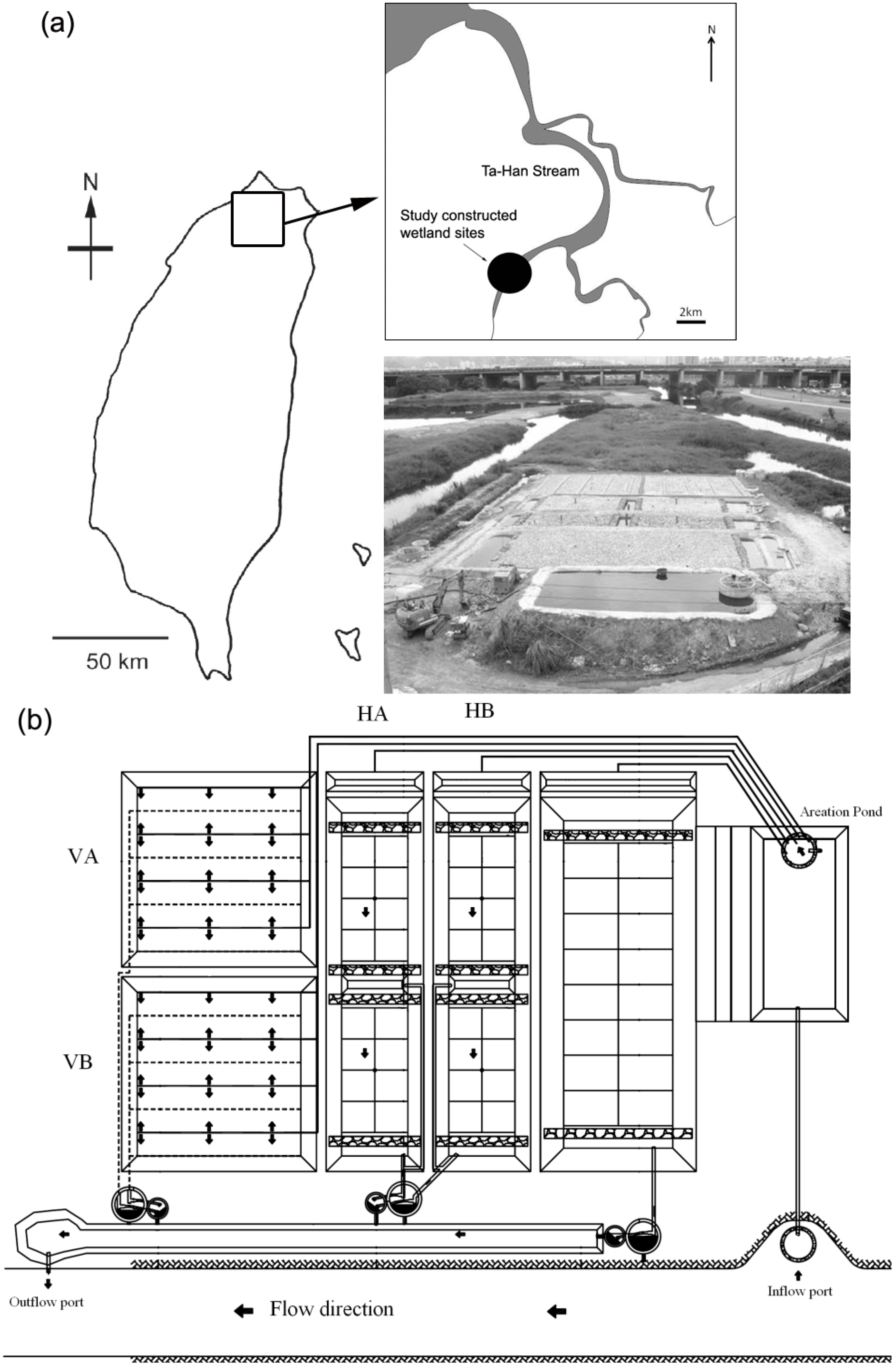
2.1.2. Configuration of the Four Study SSF CWs

In order to investigate the wastewater treatment efficiency of the oyster-shell-bedded CW systems as compared to the conventional gravel-bedded CW, we established four study SSF CWs built into two different types of water-flowing systems, including two vertical SSF CWs and two horizontal SSF CWs, packed with different arrangements of oyster shells and gravels. The two vertical SSF CWs were measured 8.4 m × 8.4 m × 1 m (L × W × D) in size and filled with oyster shells with average dimensions of 6.76 cm long, 4.23 cm wide, and 0.27 cm thick. Bagged and scattered stacking methods of oyster shells were applied to these two vertical SSF CWs named as VA and VB respectively. The original purpose of bagged oyster-shell arrangement included fixing the void ratio in the unit and stabilizing the system of filtering medium under high wastewater discharge. The two horizontal SSF CWs were named as HA and HB (Figure 1b). The dimension of each horizontal SSF constructed wetland was 12 m × 3.4 m × 1 m (L × W × D). HA wetland was filled with oyster shells as the adsorbent medium while HB wetland was a conventional gravel-bedded constructed wetland. Due to the difference in physical properties between oyster shells and gravels (Table 1), the resulting difference in the waste removal quantity between HA and HB wetlands could therefore be indicative of the waste treatment performance between these two filtering materials.

Table 1. Summary of physical properties of oyster shells and gravels [9].

Table 1. Summary of physical properties of oyster shells and gravels [9].

Item	Oyster shells	Gravels
True density (kg/m3)	1273	2283
Bulk density (kg/m3)	289	1365
Porosity (%)	77	40
Special surface area (m2/kg)	0.96	0.23
Special surface area (m2/m3)	1217	527

The inflow discharge of wastewater was maintained consistently for the four study SSF constructed wetlands, i.e., between 101 and 225 m³/day, to simulate the natural condition of Ta-Han Stream floodplain. The water outlet of each study SSF constructed wetland was designed as a gravitational jet form to increase the aeration effect. Same source of the inflow wastewater was directed to the four SSF CWs. The inflow water quality and the operation procedures of all four sites were maintained identical (Table 2). During the study period, inflow wastewater was first pumped through the aeration tank for oxygenation and allowed for precipitation as pre-treatment, it was then flowed into each study constructed wetland separately so that we could monitor the water quality of the outflow to determine the treatment efficiency and waste removal quantity of the four study SSF CWs. The purposes for the two-stage pre-treatment included removing the suspended solids through precipitation and oxidizing most of the ammonium into nitrates through aeration to enable the denitrification of nitrates into nitrogen in the anaerobic environment of the four SSF CWs.

Table 2. Water quality parameters of the wetland influent in this study.

Table 2. Water quality parameters of the wetland influent in this study.

Descriptive statistics	BOD	DO	TP	SS	NH4+	NO3−	pH	Temp
Average	14.7	2.34	0.99	32.8	9.09	0.75	7.05	28.5
SD	4.53	0.56	0.37	6.21	3.79	0.61	0.24	0.83
Maximum	27.7	3.90	1.93	65.0	24.6	2.83	7.68	32.4
Minimum	5.48	0.20	0.49	12.0	1.88	0.04	6.74	26.9

Notes: Unit of BOD, DO, NH₄⁺, NO₃⁻, TP and SS = mg/L; unit of Temp = °C.

The present work was the pioneer study of application of oyster shells as the adsorbent medium in the “real” SSF CWs, our experiment was carried out for 55 days during June 25–August 18, 2008 to provide preliminary data of the waste treatment performance and cost effectiveness of the oyster-shell-bedded constructed wetland systems. Operational data of the four study CWs were collected twice per day by measuring eight water quality parameters including temperature (°C), pH, concentrations of biochemical oxygen demand (BOD, mg/L), dissolved oxygen (DO, mg/L), total phosphorous (TP, mg/L), suspended solids (SS, mg/L), ammonium (NH₄⁺, mg/L), and nitrate (NO₃⁻, mg/L). Measurement of these water quality parameters were based on the standard methods [17].

As the inflow wastewater was dominated by organic pollutants, BOD was selected as the key parameter for assessing waste removal quantity and treatment efficiency for the organic wastewater by the four SSF CWs. The waste removal quantity and treatment efficiency were evaluated at 35-day and 55-day periods during the wetland operation. The mean hydraulic retention time (HRT) of the four SSF CWs were 0.2 day [range = 0.09 (HB)–0.28 (VB)] and 0.12 day [range = 0.07 (HB)–0.19 (VA)] at 35-day and 55-day operation periods respectively (Table 3).

Table 3. Average wastewater removal quantity (g/m³/day) and average treatment efficiency (%) and hydraulic properties of the four study wetlands calculated at 35-day and 55-day operation period in the present study.

Table 3. Average wastewater removal quantity (g/m³/day) and average treatment efficiency (%) and hydraulic properties of the four study wetlands calculated at 35-day and 55-day operation period in the present study.

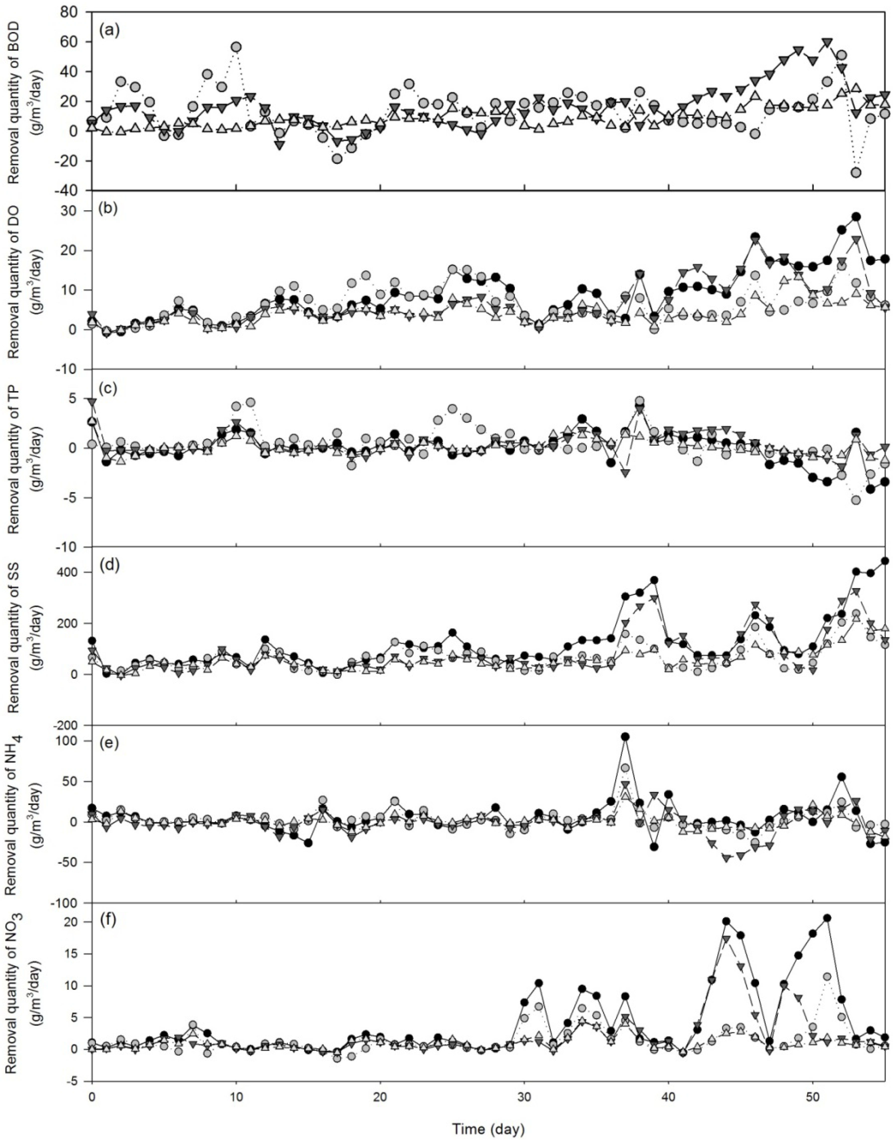
Removal quantity (g/m3/day)	BOD	DO	TP		SS		NH4+	NO3−		Q (CMD)		HRT (day)
Average wastewater removal quantity in 35 days
HA(oyster shells)	13.52	6.27	0.55		60.18		−0.91	1.50		114.98		0.16
HB(gravels)	9.81	5.59	0.89		49.65		2.19	0.61		101.21		0.09
VA(bagged oyster shells)	9.24	3.50	0.46		39.76		−0.97	0.60		122.99		0.26
VB(scattered oyster shells)	8.03	3.35	0.20		37.85		0.61	0.41		111.67		0.28
Average wastewater removal quantity in 55 days
HA	23.17	8.89	0.35		114.65		2.00	2.42		178.79		0.09
HB	12.61	5.69	0.34		64.60		−0.10	0.60		110.09		0.07
VA	21.50	6.92	0.34		100.62		−4.45	1.51		224.91		0.13
VB	17.59	4.32	0.10		57.76		−1.55	0.54		137.36		0.19
Rate (%)	BOD	DO		TP		SS			NH4+		NO3−
Average treatment efficiency in 35 days
HA	24.23	46.97		4.23		38.83			−7.53		24.32
HB	21.97	49.01		18.20		34.23			4.93		8.87
VA	24.97	44.29		5.96		39.18			−7.15		19.42
VB	19.13	49.66		−0.90		44.10			−2.67		4.82
Average treatment efficiency in 55 days
HA	22.14	47.46		1.89		41.28			−3.43		26.86
HB	19.68	49.70		5.48		38.73			−5.03		7.42
VA	28.61	49.30		3.15		43.68			−11.00		19.98
VB	22.22	51.42		−0.87		48.11			−10.60		10.90

2.1.3. Cost-Effectiveness Analysis

The total cost of wastewater treatment consists of two aspects including the capital cost (i.e., construction cost) and operation and maintenance (O&M) cost. The capital costs of our four study SSF CWs included the construction materials and building services was determined from the actual expenses involved in establishing these CWs. However, the expense of land was neglected in the present study as our field experiment was conducted on the land owned by the local Government and it was impossible to estimate the cost of land rental. As BOD is commonly regarded as an important index of wastewater treatment in Taiwan and many other countries [6,15], so the cost per mass BOD removed was selected as the measure of wastewater treatment performance in the present cost-effectiveness analysis. In our study, the BOD treatment performance was estimated during the operation time of our experimental period of 35 and 55 days. The cost-effectiveness values of the four study SSF CWs in 55-day period were calculated. However, it would be important to consider the cost-effectiveness of wastewater treatment of CWs in long-term operation. We therefore broke the capital costs into 20-year annuity (w) by the following equation:

(1)

where P is the capital cost and r is the interest rate which was assumed to be 0.05 [4]. The total costs per annuity of the four study wetlands were obtained by the summation of their capital costs per annuity and O&M costs.

2.1.4. Statistical Analysis

Data of inflow and outflow water quality of the four study SSF CWs were compared and used for determination of their wastewater treatment efficiency. Water quality data were first checked for normality and homogeneity of variance test, one-way Analysis of Variance (ANOVA) was then used to test the difference in each water chemistry parameter among the four SSF CW. Student-Newman-Keuls Post-hoc test (S-N-K test) was applied when significant among-site difference in water chemistry parameter was detected by the 1-way ANOVA. All statistical analysis was carried out using SPSS Statistics 17.0.

2.2. Simulation Model

In the CWs, biochemical reactions, such as mineralization, nitrification, respiration, biofilm adsorption, biomass decay, and sediments consumption are important wastewater treatment mechanisms [2]. Many computer programs such as CW2D [18] and WASP/EUTRO5 [19] were developed for describing complex reactions in CWs. In this study, we used the program AQUASIM 2.1, which was originally designed for identification and simulation of aquatic systems under varied situations [14]. The major reason for choosing AQUASIM was due to its flexible operational platform for easily simulation of the above biochemical processes in CWs, especially biofilm adsorption. In water quality modeling, we assumed water was well mixed in SSF CWs, so that the mixed reactor compartment, a water quality simulation tool in AQUASIM, was applied to describe well-mixed domains. Then, temporal variations of BOD, DO, TP, SS, NH₄⁺, and NO₃⁻ concentrations during the wastewater treatment processes could be then simulated. Details of the water quality operational equations, biochemical processes, five water chemistry submodels of C-cycle, O-cycle, N-cycle, P-cycle, and suspended solids from our water quality model were reported in the following sections [Table 4, Table 5; see also the definition of each process rate in Equations (2) to (7)].

Table 4. Parameters and reaction kinetics of different nutrient cycle processes involved in the CW waste treatment [20].

Table 4. Parameters and reaction kinetics of different nutrient cycle processes involved in the CW waste treatment [20].

Process rate	Definition	Rate
C-cycle
rBOD	Biochemical degradation
rR­_BOD	Microorganism respiration
rDecay_BOD	Biomass decay
rB_BOD	Biofilm adsorption
O-cycle
rDO	Biochemical degradation
rN_DO	Nitrification
rR_DO	Microorganism respiration
rSOD	Sediment consumption
rB_DO	Biofilm adsorption
P-cycle
rP	Phosphorous utilization by microorganisms
rSettling_P	Phosphorous settling
rDecay_P	Biomass decay
rB_P	Biofilm adsorption
Suspended solids
rFitration	Filtration
rSettling_SS	Settling
rDecay_SS	Biomass decay
rB_SS	Biofilm adsorption
N-cycle
rN_N	Nitrification
rG_NH4	Ammonia utilization by microorganisms
rG_NO3	Nitrate utilization by microorganisms
rReg	Ammonia regeneration
rMin	Mineralization
rDN	Denitrification
rDecay_N	Biomass decay
rB_N	Biofilm adsorption
CT*	Temp. dependent factor
CpH*	pH growth-limiting factor	If pH<7.2 then (1-0.833•(7.2-pH) ) else 1

Also, as accumulated studies on CWs have suggested that biofilm was an important factor associated with the water quality of CWs, e.g., [21,22], the biofilm reactor compartment was established in our model for estimating the biofilm population dynamics. Detailed descriptions of the model coefficients, parameters and constants of the biofilm reactor compartment are given in Table 5.

Table 5. Summary of parameters and constants of different biochemical processes of CW waste treatment involved in the simulated model (experimental data, C-cycle, O-cycle, P-cycle and SS removal, N-cycle, biofilms, temperature coefficients and half-saturation constants).

Table 5. Summary of parameters and constants of different biochemical processes of CW waste treatment involved in the simulated model (experimental data, C-cycle, O-cycle, P-cycle and SS removal, N-cycle, biofilms, temperature coefficients and half-saturation constants).

Parameter	Description	Literature range	Unit	Source
Experimental data
A	Cross-sectional area	-	m2	Field monitoring data
AS	Special surface area of media	-	m2/m3	[9]
BODd	Dissolve BOD	-	mg/L	Field monitoring data
BODs	Suspended BOD	-	mg/L	Field monitoring data
dc	Diameter of collector	-	m	Field monitoring data
H	Depth	-	m	Field monitoring data
p	Porosity	-	%	Field monitoring data
Qin	Inflow	-	m3/day	Field monitoring data
SNagger	Nitrogen in aggregates	-	mg/L	Field monitoring data
SON	Organic nitrogen	-	mg/L	Field monitoring data
C-cycle
kBOD	Biochemical degradation rate of BOD	0.3	day−1	[23]
kDecay_BOD	Biomass decay rate	0.15	day−1	[24]
ksob_BOD	Biofilm adsorption coefficient of BOD	-	m−3day−1	-
RBOD	Microorganisms respiration coefficient	-	-	-
μBOD	Max growth rate of hetero. at 20 °C	0.8–6	day−1	[25]
φBOD	Empirical constant of BOD	0.098	°C−1	[20]
O-cycle
HSDO	Sediment oxygen demand constant	2.5	mg/L	[24]
kd_C	Degradation rate for BODd	0.3	day−1	[23]
kN	Nitrification rate at 20 °C	0.05	day−1	[23]
ks_C	Degradation rate for BODs	0.3	day−1	[23]
ksed	Sedimentation coefficient	0.1	-	[23]
ksob_DO	Biofilm adsorption coefficient of DO	-	m−3day−1	-
RDO	Heterotrophic respiration coefficient	0.1	-	-
SOD	Sediment oxygen demand	0.1	gO2/m2day	[23]
μDO	Max growth rate of hetero. at 20 °C	0.015–0.2	day−1	[26,27]
φDO	Empirical constant of DO	0.098	°C−1	[20]
P-cycle
iP,BM	Phosphorus content of biomass	0.02	mgP/mgBM	[28]
kDecay_P	Biomass decay rate	0.15	day−1	[24]
kP	Biochemical degradation rate	-	day−1	-
kSettling_P	Phosphorous settling coefficient	0.03	m−1day−1	-
ksob_P	Biofilm adsorption coefficient of TP	-	m−3day−1	-
φP	Empirical constant of TP	0.098	°C−1	[20]
Suspended solids
dSS	Diameter of settling particle	0.1–4	mm	[29]
kDecay_SS	Biomass decay rate	0.15	day−1	[24]
kF	Filtration coefficient	-	-	-
kSettling_SS	Settling coefficient	-	m−3	-
ksob_SS	Biofilm adsorption coefficient of SS	-	m−3day−1	-
α	Sticking coefficient	0.0008–0.012	-	[30]
ρs	Density of settling particle	1050–1500	kg/m3	[31]
ρW	Density of water	995.69	kg/m3	[31]
νW	Kinematic viscosity of water	0.0867	m2/day	[32]
φSS	Empirical constant of SS	0.098	°C−1	[20]
N-cycle
iN,BM	Nitrogen content of biomass	0.07	mgN/mgBM	[28]
kDecay_N	Biomass decay rate	0.15	day−1	[24]
kDN	Denitrification rate at 20 °C	0–1	day−1	[33]
kG_NH4	NH4+ uptake preference factor	-	-	-
kG_NO3	NO3− uptake preference factor	-	-	-
kMin	Mineralization rate	0.0005–0.143	day−1	[34]
kN_N	Growth rate of nitrosomonas by nitrification	0.33–2.21	day−1	[35]
kReg	NH4+ regeneration rate	0.085	day−1	[36]
ksob_N	Biofilm adsorption coefficient of NH4+ and NO3−	-	m−3day−1	-
Yn	Nitrosomonas yield coefficient	0.03–0.13	mgVSS/mgN	[37]
μmax,20	Max. growth rate of bacteria at 20 °C	0.18	day−1	[38]
φN	Empirical constant	0.098	°C−1	[20]
Biofilms
bX1	Microorganism heterotroph decay rate	0.3	day−1	-
bX2	Microorganism nitrosomonas decay rate	0.3	day−1	-
DNH4	Diffusion coefficient of NH4+	1.71 × 10−4	m2/day	[39]
DNO3	Diffusion coefficient of NO3−	(4.5–27.9) × 10−6	m2/day	[40]
DTOC	TOC diffusion coefficient	1.56 × 10−5	m2/day	[41]
DX	Microorganism diffusion coefficient	-	m2/day	-
LFmodel	Biofilms thickness	-	m	Biofilm model result
XH	Heterotrophic organisms	-	mg/L	Biofilm model result
Y1	Yield constant of heterotroph	0.6	-	[27]
Y2	NH4+ yield constant of nitrosomonas	0.13	-	[27]
Y3	NO3− yield constant of nitrosomonas	0.03	-	[27]
μX1	Max growth rate of heterotroph	3–6	day−1	[28,42]
μX2	Max growth rate of nitrosomonas	0.33–2.21	day−1	[35]
Temperature coefficient
θBOD	Temp. coefficient of degradation	1.09	-	[23]
θDecay	Temp. coefficient of biomass decay	-	-	-
θR	Temp. coefficient of respiration	-	-	-
θDN	Temp. coefficient of denitrification	1.15	-	[43]
θgrowth	Temp. coefficient of microorganisms growth	1.08–1.12	-	[31]
θN	Temp. coefficient of nitrification	1.1	-	[23]
Half- saturation (Half-sat.) constant
KBOD	Half-sat. constant of BOD	2	mg/L	[23]
KDO	Half-sat. constant of DO	2	gO2/m3	[23]
KP	Half-sat. constant of TP	0.02	mg/L	[44]
Kn	Half-sat. constant of NH4+ nitrosomonas	0.05	mg/L	[23]
KnDO	Half-sat. constant of DO nitrosomonas	0.13–1.3	mg/L	[35]
KNH4	Half-sat. constant of NH4+	2	gCOD/m3	[27]
KNO3	Half-sat. constant of NO3−	0.15–0.5	gN/m3	[26,45]

2.2.1. Carbon Cycle

Organic matters usually exist in five different types in CWs, e.g., dissolved phase, suspended phase, bottom phase, biomass, and inertia carbon [45]. Microorganisms play the principal roles of organic matter removal in CWs through their utilization and respiration. The temporal and spatial variability of BOD in CWs are controlled by the following equation (Table 4, Table 5):

(2)

where I_in,BOD is loading of BOD into the reactor (mass per unit per time), V_R is the reactor volume, Q_out is the volumetric outflow, and C_BOD is the concentration of BOD. Other process rates are shown in Table 4.

2.2.2. Oxygen Cycle

DO is one of the most important water quality indicators as many biochemical processes require the participation of oxygen. As the flow velocity is relatively low and water surface area for gaseous exchange is small in SSF CWs, oxygen cannot enter its water bodies by diffusion. Moreover, there is no other aeration mechanism such as photosynthesis, root-zone effect and artificial aeration in these wetlands. Therefore, DO is further diminished by the processes associated with sediment oxygen demand, bacteria respiration, nitrification, and oxidation of BOD as described by the following equation (Table 4, Table 5):

(3)

where I_in,DO is loading of DO into the reactor (mass per unit per time), and C_DO is the concentration of DO.

2.2.3. Phosphorus Cycle

Removal rates of TP in CWs are dominated by plant uptake [28]. In addition, phosphorus can combined with heavy metal, adsorbed by suspended solids and utilized by microorganisms in wetlands. The mass balance equation for TP is given in the following (Table 4, Table 5):

(4)

where I_in,TP is loading of TP into the reactor (mass per unit per time) and C_TP is the concentration of TP.

2.2.4. Suspended Solids

Multiple physical processes relating to filtration and precipitation control the temporal variability of SS in CWs. In SSF CWs, SS can be blocked, trapped and intercepted when they pass through stems/roots of plants, sandstones, and other media. In our simulated model, we also considered the adsorption of biofilm as a momentous process for SS removal. The mass balance for SS in wetlands is given as follows (Table 4, Table 5):

(5)

where I_in,SS is loading of suspended solids into the reactor (mass per unit per time), and C_SS is the concentration of suspended solids.

2.2.5. Nitrogen Cycle

In natural environment, nitrogen involves in many biochemical processes and it exists in many different forms from the most oxidized form nitrates (NO₃⁻) to the most reduced form ammonium (NH₄⁺). Organic nitrogen in wetlands is first transformed into NH₄⁺ through mineralization, and then converted into NO₃⁻ via the two stages of nitrification [2]. During the removal process of NH₄⁺, part of the NH₄⁺ is converted into NO₃⁻ and remains in wetlands. In this study, we therefore considered dissolved nitrogen (NH₄⁺ and NO₃⁻) as the major forms of nitrogen in the study CWs. The mass balance for NH₄⁺ and NO₃⁻ are given as follows (Table 4, Table 5):

(6)

(7)

where is loading of NH₄⁺ into the reactor (mass per unit per time), is loading of NO₃⁻ into the reactor (mass per unit per time), is the concentration of NH₄⁺, and is the concentration of NO₃⁻.

2.2.6. Biofilm Reactor Compartment

The biofilm model is developed based on the one-dimensional mixed culture biofilm model [14,46] (Table 5). The one-dimensional conservation laws are formulated by AQUASIM 2.1 to describe the transmission processes of dissolved substances and suspended solids in biofilms (solid matrix and pore water). The growth or decay of organisms was expressed by the expansion or contraction of biofilms.

2.2.7. Sensitivity Analysis

The wastewater treatment efficiency in each wetland was obtained based on the monitoring data of inflow and outflow water quality in the study SSF CWs. The influence of different biochemical processes on the wastewater treatment efficiency were quantified by inputting the field monitoring data of the four wetlands into the water quality model for sensitivity analysis. The sensitivity analysis was used to determine the sensitivity and relative importance of each biochemical process [35,47]. We first applied the absolute-relative sensitivity function [Equation (8)] provided by AQUASIM to measure the sensitive value (SensAR) of each parameter:

(8)

where SensAR is sensitive value; p is a model parameter and y is a state variable.

Since BOD removal is one of the main functions of CWs and BOD loading are commonly considered as an important factor for assessing wetland operation [1,6,7], BOD was taken as the basis for the evaluation of the sensitivity of parameters in this study. Also, as identification of parameters is necessary for improving the accuracy of water quality simulations, the feasible range of all parameters in oyster-shell-bedded CWs were determined in AQUASIM.

3. Results and Discussion

3.1. Field Experiment

3.1.1. Cost-Effectiveness Analysis

The capital costs, O&M costs, total costs and cost-effectiveness in 55-day- and 20-year annuity period for each study SSF CW were shown in Table 6. The original capital costs were 19 times of the capital cost in 20-year annuity. Therefore, the capital costs made up of the majority (~97%) of the total costs of all four CWs when the operation period was 55 days. However, the capital cost per annuity was only 20% of HA, VA and VB, and 24% of HB of the total costs when these wetlands were assumed to be operated for 20 years. Moreover, the total cost for all the CWs operated for in 55-day-period [range = US$10711 (HA)–13586 (HB)] were 2.9–3.7 times higher as compared to the total cost for 20-year annuity [range = US$2737 (VB)–2869 (HB)]. Also, the cost per mass BOD removed was 25–30 times higher in all wetlands for the 55-day than 20-year annuity period. Our results highlighted that the economic returns of CWs would be higher for long-term operation.

Among the four study SSF CWs, the capital cost and total cost of gravel bedded site HB were 16%–28% higher than the other three filled with oyster shells. However, the total BOD removal quantity of HB was only one forth to half of HA, VA and VB. Our results showed that, upon long term operation (20-year annuity), the treatment cost of 1kg BOD was US$25.01 in HB but only US$6.56 was required for VA wetland. VA also demonstrated the highest cost-effectiveness among the three oyster-shell filled CW systems (HA = US$13.04; VB = US$10.88). This confirmed that oyster shells were the cost-effective adsorption medium in SSF CW as compared to the conventional gravel-bedded SSF CW.

Table 6. Results of cost-effectiveness analysis of the four study SSF CWs.

Table 6. Results of cost-effectiveness analysis of the four study SSF CWs.

Cost	HA	HB	VA	VB
Capital cost
Suppose engineering	916	987	1046	1046
Civil engineering	570	614	651	651
Pumping well	254	273	290	290
Aeration pond	851	916	971	971
Diversion cut	1740	1880	0	0
Reverse-flushing system	1260	1167	0	0
Water distribution pipe	0	0	560	560
Sludge pipe	0	0	1700	1700
Antiseep engineering	1406	1514	1606	1606
Collection drains	1960	2111	2239	2239
Media paving	282	303	322	322
Water quality monitoring pipe	133	133	100	100
Gravels	0	3360	0	0
Oyster shell transport	1007	0	1007	1007
Bagged	0	0	984	0
Original capital cost (US$)	10379	13258	11475	10491
Capital cost—20-year annuity (US$/yr)	545	696	602	551
O&M cost
55-day-operation-period (US$)	332	328	335	329
Per year (US$/yr)	2205	2173	2226	2186
Total cost
55-day-operation-period (US$)	10711	13586	11810	10820
20-year annuity (US$/yr)	2749	2869	2828	2737
Total waste removal quantity of BOD during the operation time
55-day-operation-period (kg)	31.77	17.29	64.97	37.92
Per year (kg/yr)	210.83	114.74	431.17	251.63
Cost-effectiveness value (Cost per mass BOD removed)
55-day-operation-period (US$/kg)	337.15	785.79	181.78	285.38
20-year annuity (US$/kg)	13.04	25.01	6.56	10.88

3.1.2. Treatment Efficiency Analysis

As no macrophyte was planted in the four study SSF CWs, the wastewater treatment mechanisms were dominated by physical deposition and biochemical decomposition, including settling, filtration, regeneration, nitrification, denitrification, mineralization, sediment consumption, biomass decay, microorganism respiration, biochemical degradation, biofilm adsorption, and microorganism utilization. The waste removal quantity of BOD, DO, TP, SS, NH₄⁺, and NO₃⁻ showed inconsistent trend in HA, HB, VA, and VB wetlands during our study period (Figure 2a–f; Table 7). Removal quantity of BOD, SS and NO₃⁻ were higher in HA and VA wetlands. But, the removal of TP was not significant in these wetlands. In wastewater purification processes, DO was consumed continuously by the aerobic biochemical reactions, resulting in the low DO concentration in outflow from all four wetlands (Figure 2b).

The average waste removal quantity of most wastewater parameters increased slightly from 35-day to 55-day-periods but the average treatment efficiency of all wastewater parameters remained fairly constant between 35-day and 55-day-periods. Our preliminary findings suggested that increasing the operation time could enhance the success of CWs in terms of wastewater treatment efficiency. However, further confirmation would be needed for the four types of study CWs in Taiwan by extending the length of study period.

Figure 2. Waste removal quantity (g/m³/day) of (a) oxygen demand (BOD); (b) dissolved oxygen (DO); (c) total phosphorous (TP); (d) suspended solids (SS); (e) NH₄⁺; and (f) NO₃⁻ in the four study SSF wetlands (HA = black circles; HB = grey circles; VA = inverted grey triangle; VB = white triangle).

Table 7. Results of one-way Analysis of Variance (ANOVA) assessing the waste removal quantity of each wastewater parameter among the four study SSF CWs. * p < 0.05.

Table 7. Results of one-way Analysis of Variance (ANOVA) assessing the waste removal quantity of each wastewater parameter among the four study SSF CWs. * p < 0.05.

Wastewater parameter	F-value	P-value
BOD	2.655	0.049*
DO	8.498	0.000*
TP	0.380	0.767
SS	6.727	0.000*
NH4+	1.388	0.247
NO3−	4.233	0.006*

Our results highlighted that there were significant differences in the waste removal quantity of BOD, DO, NO₃⁻, SS among the four wetlands (BOD: F_{3, 220} = 2.655, p = 0.049; DO: F_{3, 220} = 8.498, p < 0.001; NO₃⁻: F_{3, 220} = 4.233, p = 0.006; SS: F_{3, 200} = 6.727, p < 0.001) (Table 7). Post-hoc S-N-K comparisons between HA and HB wetlands showed that waste removal quantity in HA (23.17 g/m³/day for BOD, 2.42 g/m³/day for NO₃⁻, and 114.65 g/m³/day for SS) was significantly higher than HB (12.61 g/m³/day for BOD, 0.6 g/m³/day for NO₃⁻, and 64.6 g/m³/day for SS) (Table 3). Thus, the treatment efficiency of HA was higher than HB in BOD, NH₄⁺, NO₃⁻, and SS. However, the BOD, NO₃⁻, DO and SS treatment efficiency of both HA and HB were lower than VA and VB primarily due to the difference in the site infrastructure (Figure 1b) and the size of biofilm reactor compartment (VA and VB > HA and HB).

Comparing HA and VB wetlands, HA had 1.92 g/m³/day NO₃⁻ and 56.89 g/m³/day SS of waste removal quantity which were significantly higher than VB. However, VB showed slightly higher treatment efficiency than HA because the reactor volume of VB was larger than HA. On the other hand, despite the SS removal quantity in VA wetland was significantly higher than VB (100.62 g/m³/day and 57.76 g/m³/day respectively) (Table 3, Table 8), treatment efficiency of SS remained relatively similar among the four study CWs.

Table 8. Results of sensitivity analysis of BOD removal quantity from all biochemical processes in the simulated model.

Table 8. Results of sensitivity analysis of BOD removal quantity from all biochemical processes in the simulated model.

Parameters	SensAR		SensAR		SensAR		SensAR
	RMS	Mean	RMS	Mean	RMS	Mean	RMS		Mean
	HA		HB		VA			VB
ksob_BOD	3.535	−3.086	0.920	−0.794	3.341	−3.053	3.338		−3.179
kDecay_BOD	1.578	1.392	0.571	0.538	1.753	1.663	0.958		0.930
kBOD	0.556	−0.492	1.856	−1.713	0.098	0.083	0.280		−0.257
RBOD	0.274	−0.231	0.009	0.004	0.146	−0.241	0.204		−0.187

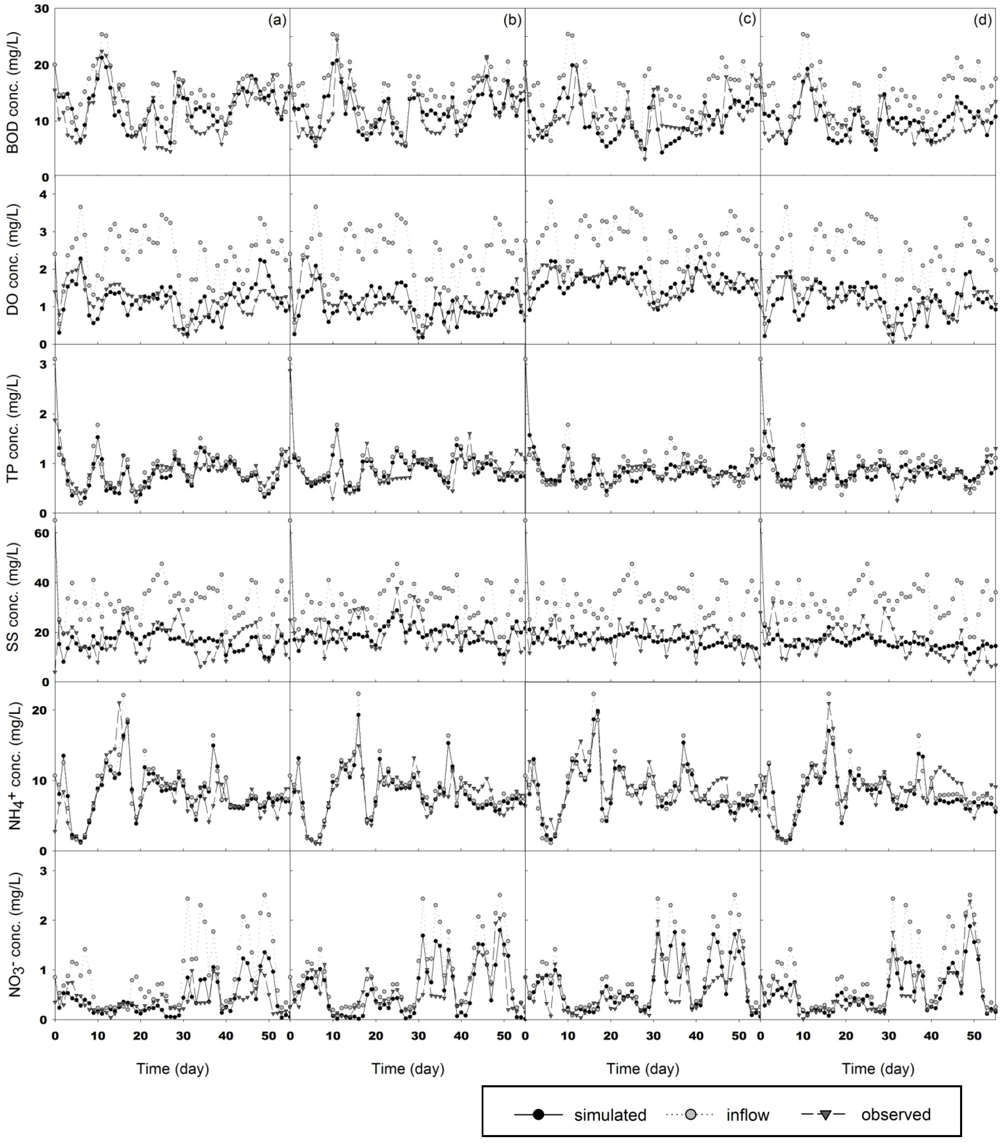
Comparison between bagged (VA) and scattered (VB) arrangement oyster-shell-bedded CW indicated that the waste removal quantity and treatment efficiency between these two wetlands were generally similar. However, VA wetland demonstrated significantly highest BOD treatment efficiency among all study CWs. Our results indicated that oyster shells were an effective adsorption medium in SSF CW because of its lower cost and better wastewater treatment performance as compared to the conventional gravel-bedded SSF CW. But, the site infrastructure, hydraulic patterns and arrangement of oyster shells could be important in determining the waste removal efficiency and cost-effectiveness of CWs. The observed effectiveness of oyster shells as biofilter substrates in CWs due to their higher porosity and surface area/volume ratio as compared to gravels, and thus providing larger contact area for efficient nutrient treatment (Table 1) [9].

In addition, as denitrification usually occurs in low dissolved oxygen or anaerobic conditions because denitrifying bacteria are usually anaerobic and heterotrophic, the efficiency of denitrification is also limited by the source of carbon in the environment [48]. Among the four study wetlands, HA showed the highest NO₃⁻ removal efficiency probably due to its low DO environment (Figure 3). In general, horizontal SSF CWs were predominantly anaerobic, but the oxygen supply is usually higher in vertical SSF CWs which show higher rates of bio-decomposition of organic carbon [49]. This could therefore explain the higher BOD removal efficiencies in VA and VB wetlands.

Figure 3. Simulated BOD, DO, TP, SS, NH₄⁺ and NO₃⁻ outflow results and measured data in (a) HA; (b) HB; (c) VA; and (d) VB wetlands.

3.2. Simulation

3.2.1. Sensitivity Analysis

The biofilm adsorption coefficient of BOD (k_{sob_BOD}) had the highest SensAR in most of the treatment units except for the gravel-bedded constructed wetland (HB) among the four key parameters (k_{sob_BOD}, k_{Decay_BOD}, k_BOD and R_BOD) (Table 8). This suggested that the biofilm adsorption was the most effective process for BOD removal quantity in all three oyster-shell-bedded wetlands (i.e., HA, VA and VB wetlands) as SensAR represented the waste removal quantity of each biochemical processes (Table 8). Hence, biofilm adsorption was the major mechanism for wastewater treatment in the three oyster-shell-bedded CWs as previous studies confirmed that oyster shells provided more area for microbial propagation than gravels [50,51]. Therefore, the treatment efficiency in CWs can be enhanced by using oyster shells as an adsorption medium.

3.2.2. Feasible Range of Parameters in Oyster-Shell-Bedded CWs

Field monitoring data of water quality from the three oyster-shell-bedded CWs were input to the water quality model to determine the feasible range of each parameter. In this part, we avoided changing values of constants such as half-saturation constant, max growth rate of bacteria, and others, which were obtained from microorganism experiments. Thus, three sets of parameters were obtained by model fitting of the experimental data of the three oyster-shell-bedded wetlands. The model fitting results of HA, VA, and VB wetlands are given in Figure 3.

For the three sets of parameters, we took the maximum value as the upper bound and the minimum value as the lower bound of each parameter. The upper and lower bounds were integrated to set the feasible range of each parameter in Table 9. The feasible range could provide a reference for simulation and prediction in further studies.

Table 9. Feasible range of parameters in the oyster-shell bedded CWs.

Table 9. Feasible range of parameters in the oyster-shell bedded CWs.

Submodel	Parameter	HA	VA	VB	Feasible range
C-cycle	kBOD	0.680	0.894	0.752	0.680–0.894
	kDecay_BOD	5.977	8.764	9.335	5.977–9.335
	ksob_BOD	12.65	34.13	32.69	12.65–34.13
	RBOD	6.704	17.97	13.08	6.704–17.97
	θBOD	0.931	0.898	0.826	0.826–0.931
	θDecay	0.794	0.764	0.706	0.706–0.794
	θR	0.729	0.771	0.745	0.729–0.771
	μBOD	3.000	3.000	3.000	3.000
	φBOD	0.081	0.104	0.097	0.081–0.104
O-cycle	HSDO	3.000	3.000	3.000	3.000
	kd_C	0.076	0.268	0.010	0.010–0.268
	kN	0.001	0.001	0.001	0.001
	ks_C	0.578	1.001	0.572	0.572–1.001
	ksed	0.921	0.742	0.897	0.742–0.897
	ksob_DO	23.36	26.14	45.01	23.36–45.01
	RDO	10.55	23.02	8.224	8.224–10.56
	SOD	0.100	0.100	0.100	0.100
	θBOD	0.905	0.759	0.854	0.759–0.905
	θN	0.688	0.600	0.600	0.600–0.688
	θR	0.881	0.836	0.799	0.799–0.881
	μDO	0.163	0.163	0.163	0.163
	φDO	0.010	0.010	0.010	0.010
P-cycle	iP, BM	0.020	0.020	0.020	0.020
	kDecay_P	5.662	11.68	10.83	5.662–11.68
	kP	0.472	2.127	0.921	0.472–2.127
	kSettling_P	0.020	0.025	0.024	0.020–0.025
	ksob_P	0.058	0.593	0.309	0.058–0.593
	θDecay	0.725	0.903	0.848	0.725–0.903
	θR	0.757	0.718	0.742	0.718–0.757
	φP	0.130	0.127	0.092	0.092–0.130
SS	dSS	0.001	0.001	0.001	0.001
	kDecay_SS	1.514	3.937	2.413	1.514–3.937
	kF	0.007	0.017	0.007	0.007–0.017
	kSettling_SS	0.100	0.300	0.315	0.100–0.315
	ksob_SS	8.390	16.74	28.24	8.390–28.24
	Sg	1500	1500	1500	1500
	α	0.007	0.007	0.007	0.007
	ρS	1300	1300	1300	1300
	ρW	995.7	995.7	995.7	995.7
	νW	0.087	0.087	0.087	0.087
	θDecay	1.043	0.996	1.028	0.996–1.043
	φSS	0.018	0.134	0.010	0.010–0.134
N-cycle	iN, BM	0.070	0.070	0.070	0.070
	kDecay_N	0.035	0.086	0.178	0.035–0.178
	kDN	1.582	0.051	0.771	0.051–1.582
	kG_NH4	0.354	0.032	0.032	0.032–0.354
	kG_NO3	0.727	2.934	2.477	0.727–2.934
	kMin	0.100	0.569	0.228	0.100–0.569
	kN_N	0.873	0.808	0.915	0.808–0.915
	kReg	0.100	0.731	0.291	0.100–0.731
	ksob_N	0.934	1.498	1.347	0.934–1.498
	Yn	0.130	0.130	0.130	0.130
	φP	0.130	0.127	0.092	0.092–0.130
	θDecay	0.894	0.852	0.882	0.852–0.884
	θDN	1.181	1.198	0.958	0.958–1.198
	θGrowth	0.871	0.903	0.900	0.871–0.903
	θN	0.939	0.768	0.77	0.768–0.939
	μmax,20	0.180	0.180	0.180	0.180
	φN	0.098	0.098	0.098	0.098

3.2.3. Applications of Our Model

Many wetland models presented previously often used diffusion coefficient in sublayer (m²/day), diffusivity of substrate in biofilm (m²/day), and sublayer thickness (m), along with the experiment results of the biofilm thickness (from 1.46 × 10⁻³ to 1.62 × 10⁻³ m), to estimate reaction of biofilm adsorption [36,50]. In contrast, our model utilized the biofilm compartment in AQUASIM to perform an initial dynamic modeling of the biofilm time variation, as one of the referencing conditions for water quality modeling. After that, a sensitivity analysis on different influential factors was carried out to identify the significant biofilm biochemical mechanisms for water quality improvement.

4. Conclusions

(1)

The four study SSF CWs showed a significant difference in the waste removal quantity of BOD, DO, NO₃⁻, and SS. The waste removal quantity of the horizontal SSF oyster-shell-bedded CW (HA) was significantly higher than the horizontal SSF gravel-bedded CW (HB) but similar to the vertical SSF oyster-shell CW (VB). Comparison between bagged (VA) and scattered (VB) arrangement oyster-shell-bedded CWs indicated that the waste removal quantity and treatment efficiency between these two wetlands were generally similar. However, VA wetland demonstrated significantly highest BOD removal capacity among all study sites but also showing the lowest cost per mass BOD removed (6.56 US$/kg) as compared to other three CWs (10.88–25.01 US$/kg). Therefore, VA was determined as the best option for SFF CW in terms of waste treatment efficiency and cost-effectiveness.

(2)

The total costs of the four study CWs ranged from 2,737 (VB) to 2,869 (HB) US$/yr in 20-year annuity whereas they were between 10,711 (HA) and 13,586 (HB) US$ for only 55-day operation period. Also, the relative importance of capital costs to the total costs of all CWs for long-term operation (20-year annuity) was only one fifth of that for 55 days’ operation. Therefore, results of the cost-effectiveness analysis highlighted that the economic returns of CWs would be higher for long-term operation.

(3)

The average waste removal quantity of most wastewater parameters increased slightly from 35-day to 55-day-periods but the average treatment efficiency of all wastewater parameters remained fairly constant between 35-day and 55-day-periods. Our findings suggested that establishment time could be critical for the success of CWs with respect to wastewater treatment efficiency.

(4)

The results of our numerical water quality model demonstrated that, biofilm adsorption played the most essential role in the wastewater treatment processes in oyster-shell-bedded CWs but biochemical degradation was the most significant mechanism in gravel-bedded CW.

(5)

The feasible range of each water quality parameter in oyster-shell bedded wetlands was identified in the present study, and it was obtained by a regression model using the field monitoring data. These feasible ranges could be used for water quality simulations in the CWs and this could help characterizing different CWs by determining the quantitative importance of different biochemical treatment processes in SSF CWs.

References

1. Economopoulou, M.A.; Tsihrintzis, V.A. Design methodology and area sensitivity analysis of horizontal subsurface flow constructed wetlands. Water Resour. Manag. 2003, 17, 147–174. [Google Scholar] [CrossRef]
2. Vymazal, J.; Brix, H.; Cooper, P.F.; Haberl, R.; Perfler, R.; Laber, J. Removal Mechanisms and Types of Constructed Wetlands. In Constructed Wetlands for Wastewater Treatment in Europe; Backhuys: Leiden, The Netherland, 1998; pp. 17–66. [Google Scholar]
3. Vymazal, J. Constructed wetlands for wastewater treatment. Water 2010, 2, 530–549. [Google Scholar] [CrossRef]
4. Teng, C.J.; Leu, S.Y.; Ko, C.H.; Fan, C.; Sheu, Y.S.; Hu, H.Y. Economic and environmental analysis of using constructed riparian wetlands to support urbanized municipal wastewater treatment. Ecol. Eng. 2012, 44, 249–258. [Google Scholar] [CrossRef]
5. Chen, G.Q.; Shao, L.; Chen, Z.M.; Li, Z.; Zhang, B.; Chen, H.; Wu, Z. Low-carbon assessment for ecological wastewater treatment by a constructed wetland in Beijing. Ecol. Eng. 2011, 37, 622–628. [Google Scholar]
6. U.S. Environmental Protection Agency (USEPA), Wastewater Technology Fact Sheet Wetlands: Subsurface Flow; EPA 832-F-00-023; Office of Water, USEPA: Washington, DC, USA, 2000.
7. U.S. Environmental Protection Agency (USEPA), Manual Constructed Wetlands Treatment of Municipal Wastewaters; EPA 625-R-99-010; USEPA: Cincinnati, OH, USA, 2000.
8. Hsu, Y.F.; Pan, W.C. Study on the Production and Labor of Oyster-Cultivating Industry in Tong-Shih: A Periphery in the Commodity Chain. In Nanhua University Policy Research; Nanhua University: Chiayi, Taiwan, 2003; pp. 105–138. [Google Scholar]
9. Lin, Y.F.; Jing, S.R. Recycling of Seafood Solid Waste as Substrate Material Used in Constructed Wetland for Wastewater Treatment; National Sciences Council: Taipei, Taiwan, 2006. [Google Scholar]
10. Chen, B.; Chen, Z.M.; Zhou, Y.; Zhou, J.B.; Chen, G.Q. Emergy as embodied energy based assessment for local sustainability of a constructed wetland in Beijing. Commun. Nonlinear Sci. Numer. Simul. 2009, 14, 622–635. [Google Scholar]
11. Seo, D.C.; Cho, J.S.; Lee, H.J.; Heo, J.S. Phosphorus retention capacity of filter media for estimating the longevity of constructed wetland. Water Res. 2005, 39, 2445–2457. [Google Scholar]
12. Park, W.H.; Polprasert, C. Roles of oyster shells in an integrated constructed wetland system designed for P removal. Ecol. Eng. 2008, 34, 50–56. [Google Scholar]
13. Huett, D.O.; Morris, S.G.; Smith, G.; Hunt, N. Nitrogen and phosphorus removal from plant nursery runoff in vegetated and unvegetated subsurface flow wetlands. Water Res. 2005, 39, 3259–3272. [Google Scholar]
14. Reichert, P. AQUASIM 2.0: Computer Program for the Identification and Simulation of Aquatic Systems; Swiss Federal Institute for Environmental Science and Technology (EAWAG): Dübendorf, Switzerland, 1998. [Google Scholar]
15. Environmental Protection Administration, Republic of China (ROCEPA). Environmental Water Quality Information; ROCEPA: Taipei, Taiwan, 2010. Available online: http://wq.epa.gov.tw/WQEPA/Code/?Languages=en (accessed on 1 February 2013).
16. Chang, C.F. Economical Analysis of Oyster Shells Contact Bed in Wastewater Treatment. M.S. Thesis, National Taiwan University, Taipei, Taiwan, 2009. [Google Scholar]
17. APHA, Standard Methods for Examination of Water and Wastewater, 20th ed.; American Public Health Association, American Water Works Association, Water Environment Federation: Washington, DC, USA, 1998.
18. Henrichs, M.; Langergraber, G.; Uhl, M. Modelling of organic matter degradation in constructed wetlands for treatment of combined sewer overflow. Sci. Total Environ. 2007, 380, 196–209. [Google Scholar]
19. Yang, C.P.; Kuo, J.T.; Lung, W.S.; Lai, J.S.; Wu, J.T. Water quality and ecosystem modeling of tidal wetlands. J. Environ. Eng. 2007, 133, 711–721. [Google Scholar]
20. Downing, A.L. Population Dynamics in Biological System. In Proceedings of 3rd International Conference of Water Pollution Research, Munich, Germany, 1966; Volume 2, pp. 117–137.
21. Ottova, V.; Balcarova, J.; Vymazal, J. Microbial characteristics of constructed wetlands. Water Sci. Tech. 1997, 35, 117–123. [Google Scholar]
22. Fountoulakis, M.S.; Terzakis, S.; Chatzinotas, A.; Brix, H.; Kalogerakis, N.; Manios, T. Pilot-scale comparison of constructed wetlands operated under high hydraulic, loading rates and attached biofilm reactors for domestic wastewater treatment. Sci. Total Environ. 2009, 407, 2996–3003. [Google Scholar]
23. Lopes, J.F.; Silva, C. Temporal and spatial distribution of dissolved oxygen in the Ria de Aveiro lagoon. Ecol. Model. 2006, 197, 67–88. [Google Scholar] [CrossRef]
24. Hull, V.; Parrella, L.; Falcucci, M. Modelling dissolved oxygen dynamics in coastal lagoons. Ecol. Model. 2008, 211, 468–480. [Google Scholar]
25. Lin, T.S. The Effect of Variation of Tank Volume on Heterotrophic/Nitrifying Species in TNCU3 Activated Sludge Process. M.S. Thesis, Chaoyang University of Technology, Taichung, Taiwan, 2005. [Google Scholar]
26. Wynn, T.M.; Liehr, S.K. Development of a constructed subsurface-flow wetland simulation model. Ecol. Eng. 2001, 16, 519–536. [Google Scholar]
27. Reichert, P.; Borchardt, D.; Henze, M.; Rauch, W.; Shanahan, P.; Somlyody, L.; Vanrolleghem, P. River water quality model No. 1 (RWQM1): II. Biochemical process equations. Water Sci. Tech. 2001, 43, 11–30. [Google Scholar]
28. Henze, M. Wastewater Treatment: Biological and Chemical Processes; Springer: Berlin, Germany, 2002. [Google Scholar]
29. Poirier, M.R. Minimum Velocity Required to Transport Solid Particles from the 2H-Evaporator to the Tank Farm. Westinghouse Savannah River Company: Aiken, SC, USA, 2000; WSRC-TR-2000-00263. [Google Scholar]
30. Polprasert, C.; Khatiwada, N.R. An integrated kinetic model for water hyacinth ponds used for wastewater treatment. Water Res. 1998, 32, 179–185. [Google Scholar]
31. Tchobanoglous, G.; Burton, F.L. Wastewater Engineering:Treatment, Disposal, and Reuse; McGraw-Hill: New York, NY, USA, 1991. [Google Scholar]
32. Young, D.F.; Munson, B.R.; Okiishi, T.H.; Huebsch, W.W. A Brief Introduction to Fluid Mechanics; John Wiley & Sons: New York, NY, USA, 2010. [Google Scholar]
33. Baca, R.G.; Arnett, R.C. A Limnological Model for Eutrophic Lakes and Impoundments; Battelle, Pacific Northwest Laboratories, for USEPA, Office of Research and Development: Richland, WA, USA, 1976. [Google Scholar]
34. Martin, J.F.; Reddy, K.R. Interaction and spatial distribution of wetland nitrogen processes. Ecol. Model. 1997, 105, 1–21. [Google Scholar]
35. Jørgensen, S.E.; Nielsen, S.N.; Jørgensen, L.A. Handbook of Ecological Parameters and Ecotoxicology; Elsevier: Amsterdam, The Netherland, 1991. [Google Scholar]
36. Mayo, A.W.; Bigambo, T. Nitrogen transformation in horizontal subsurface flow constructed wetlands I: Model development. Phys. Chem. Earth. 2005, 30, 658–667. [Google Scholar] [CrossRef]
37. Charley, R.C.; Hooper, D.G.; McLee, A.G. Nitrification kinetics in activated-sludge at various temperatures and dissolved-oxygen concentrations. Water Res. 1980, 14, 1387–1396. [Google Scholar]
38. Ferrara, R.A.; Harleman, D.R.F. Dynamic nutrient cycle model for waste stabilization ponds. J. Environ. Eng. ASCE. 1980, 106, 37–54. [Google Scholar]
39. Thibodeaux, L.J. Environmental Chemodynamics:Movement of Chemicals in Air, Water, and Soil; John. Wiley & Sons: New York, NY, USA, 1996. [Google Scholar]
40. Hill, D. Diffusion-coefficients of nitrate, chloride, sulfate and water in cracked and uncracked chalk. J. Soil Sci. 1984, 35, 27–33. [Google Scholar]
41. Domingos, R.F.; Benedetti, M.F.; Croué, J.P.; Pinheiro, J.P. Electrochemical methodology to study labile trace metal/natural organic matter complexation at low concentration levels in natural waters. Anal. Chim. Acta 2004, 521, 77–86. [Google Scholar] [CrossRef]
42. Henze, M. Activated Sludge Models ASM1, ASM2, ASM2d and ASM3; IWA Publishing: London, UK, 2000. [Google Scholar]
43. Reed, S.C.; Crites, R.W.; Middlebrooks, E.J. Natural Systems for Waste Management and Treatment; McGraw-Hill: New York, NY, USA, 1998. [Google Scholar]
44. Ghermandi, A.; Vandenberghe, V.; Benedetti, L.; Bauwens, W.; Vanrolleghem, P.A. Model-based assessment of shading effect by riparian vegetation on river water quality. Ecol. Eng. 2009, 35, 92–104. [Google Scholar] [CrossRef]
45. Henze, M.; Gujer, W.; Mino, T.; Matsuo, T.; Wentzel, M.C.; Marais, G.V.R.; van Loosdrecht, M.C.M. Activated sludge model No.2d, ASM2d. Water Sci. Tech. 1999, 39, 165–182. [Google Scholar]
46. Wanner, O.; Reichert, P. Mathematical modeling of mixed-culture biofilms. Biotechnol. Bioeng. 1996, 49, 172–184. [Google Scholar] [CrossRef]
47. Wang, Y.C.; Lin, Y.P.; Huang, C.W.; Chiang, L.C.; Chu, H.J.; Ou, W.S. A system dynamic model and sensitivity analysis for simulating domestic pollution removal in a free-water surface constructed wetland. Water Air Soil Pollut. 2012, 223, 2719–2742. [Google Scholar]
48. Her, J.J.; Huang, J.S. Influences of carbon surface and C/N ratio on nitrate nitrite denitrification and carbon breakthrough. Bioresour. Technol. 1995, 54, 45–51. [Google Scholar] [CrossRef]
49. Luederitz, V.; Eckert, E.; Lange-Weber, M.; Lange, A.; Gersberg, R.M. Nutrient removal efficiency and resource economics of vertical flow and horizontal flow constructed wetlands. Ecol. Eng. 2001, 18, 157–171. [Google Scholar] [CrossRef]
50. Bouwer, E.J. Theoretical investigation of particle deposition in biofilm systems. Water Res. 1987, 21, 1489–1498. [Google Scholar] [CrossRef]
51. Tufenkji, N.; Elimelech, M. Correlation equation for predicting single-collector efficiency in physicochemical filtration in saturated porous media. Environ. Sci. Technol. 2004, 38, 529–536. [Google Scholar] [CrossRef]
52. Dixon, A.; Simon, M.; Burkitt, T. Assessing the environmental impact of two options for small-scale wastewater treatment: Comparing a reedbed and an aerated biological filter using a life cycle approach. Ecol. Eng. 2003, 20, 297–308. [Google Scholar] [CrossRef]