1. Introduction
Urban stormwater runoff is defined as the overland flow that occurs after a precipitation event in urbanized areas. These areas are characterized by a higher fraction of impervious surfaces as compared to natural, undeveloped areas. An increase in impervious surfaces, such as roofs, roads and parking lots can lead to higher runoff volumes with higher flow rates, lower evapotranspiration and lower infiltration [
1]. This can increase the risk of flooding in downstream waterways and contribute to the degradation of water quality; in fact urban stormwater runoff is considered to be a leading cause of degradation of surface waters [
2,
3,
4]. In response to the detrimental effects of runoff, a site design strategy known as Low Impact Development (or LID), has been widely adopted and aims to control, capture and treat runoff at the source and promotes sustainable water management [
5]. For LID, structural and non-structural practices are implemented on site such that the post-development hydrology and water quality mimics or improves from the pre- or undeveloped conditions [
3,
6,
7].
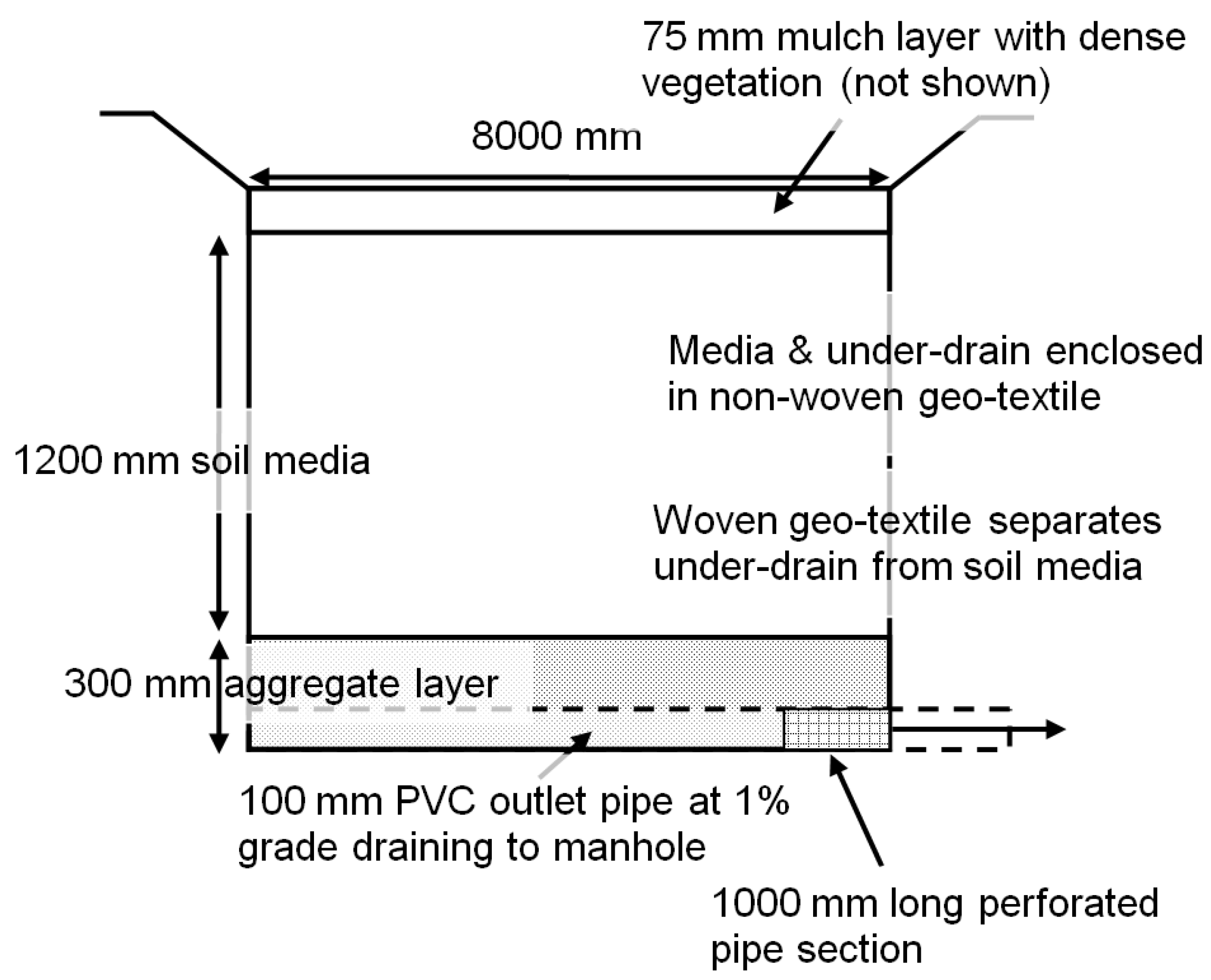
Bioretention cells, also known as rain gardens, are small, terrestrial, soil and plant based infiltration and treatment basins. They consist of a highly porous engineered soil media topped with dense vegetation and organic ground cover (such as mulch) (see
Figure 1 for a schematic of the bioretention cell used in this study). Urban runoff is routed to the cell, where it infiltrates into the media. The runoff can exit the cell via an under-drain beneath the cell, percolate into the surrounding sub-soils, or a combination of both depending on the design [
7]. The surface layer acts to attenuate the peak discharge and time of concentration of the incoming flow [
8,
9] as well as to provide storage if the runoff intensity is higher than the infiltration capacity. Losses to the surrounding sub-soils, plant uptake and storage in soil media contribute to runoff volume reduction.
Figure 1.
An example of a bioretention cell in Calgary, Canada.
Figure 1.
An example of a bioretention cell in Calgary, Canada.
Bioretention cells are used to address both runoff quantity and quality concerns. This paper will focus only on the quantity (
i.e., hydrological) component, specifically the ability of a bioretention cell to decrease or capture the amount of runoff it receives. Other hydrological performance indicators include the change in peak flow rate and the lag time of the outlet hydrograph. The ability of a bioretention cell to decrease or capture runoff volume has been reported in a number of studies. Experiments on both the field and laboratory scale have shown that the cells can capture 100% of influent volumes from small to medium size events, and between 33%–80% for larger events [
5,
10,
11,
12]. The large variability in performance in these studies can be attributed to the fact that current design guidelines are highly empirical and are not optimized for region specific differences in geological characteristics and climatic conditions [
1]. Thus bioretention cells may not perform with the same efficacy as intended if implemented without considerations for regional differences.
A number of bioretention cell design guidelines have been developed in the United States; a summary of some of these has been provided in [
13]. In most cases, the functionality of these guidelines is limited by location and climate, as described above. This is especially poignant in cold climate regions, particularly in prairie regions, where bioretention cell hydrology is unique [
14,
15]. Cold climate conditions are characterized by frozen soil, higher snowmelt volumes and lower runoff intensity from snowmelt, and repeating freeze-thaw cycles [
15]. Thus, guidelines developed in warm or temperate regions may not be applicable in cold regions.
To overcome these limitations, a number of physically-based numerical models have been created to predict bioretention cell performance [
13]. The overall objective of these models is to ascertain whether a particular design guideline is appropriate for the desired application or performance targets. Additionally, these models can predict the effects of design changes on performance. Examples include the RECARGA [
16] and RECHARGE [
17] models, based on the Richards and Green-Ampt equations, respectively. The models were developed in Wisconsin, USA and they have been adopted by the state government [
13]. Heasom
et al. [
18] developed a model using the HEC-HMS system that treats the bioretention cell as a reservoir and uses a weir system to control the outflow. Similar rainfall-runoff approach models were created using SWMM by [
19,
20].
However, a major drawback of using physically-based models is the data needed for simulations, which may not be easily available, as well difficulties in model calibration. This is especially true when a number of “sub-models” representing different processes (e.g., rainfall-runoff, infiltration, evapotranspiration) are lumped together [
21]. In addition to this, it may be difficult to mimic local characteristics using these models, for example, the frequent freeze-thaw cycles experienced in regions like Calgary, Canada. In contrast to physically-based models, data-driven models are based on the analysis of the data characterizing a system,
i.e., the bioretention cell, with limited or no assumptions regarding the nature of the physical system being modeled. Typically, the model is defined on the basis of the connections between concurrent input and output variables [
21]. An advantage of this approach is that, there is potential for establishing strong relationships between bioretention cell performance (
i.e., the output variable) and widely available input variables (e.g., precipitation depth or air temperature). If so, the ability to predict bioretention cell performance may be much simpler than relying on physically-based models that require more intensive and specialized data requirements. By using region-specific data, a data-driven model offers the potential of predicting bioretention cell performance in that region.
In this paper, a data-driven model is proposed to predict region-specific bioretention cell performance in Calgary, Canada. The use of a bioretention cell to address stormwater runoff concerns has been explored in Calgary [
15,
22]. However, to date, no comprehensive regional design guidelines or numerical models (data-driven or other) have been developed for bioretention cell use in Calgary. The city is characterized by prairie hydrology that experiences frequent freeze-thaw cycles through the winter months. These unique characteristics require specific considerations in design guidelines before widespread bioretention implementation can occur. The objectives of this research are to simulate bioretention cell performance using a data-driven model and then to use the results from the simulations to create a design tool to assist in sizing bioretention cells to meet performance targets. The research presented here uses data from Calgary; however this methodology can be applied to develop region-specific tools for any location.
The model described in this paper uses experimental data from a bioretention cell to construct and validate a multiple linear regression (MLR) model. The regressors were selected based on statistical analysis of the available parameters collected via field-scale experiments. The best performing model was used to predict bioretention cell performance under different conditions, using historical observations. These processes are described in detail below.
3. Experimental and Data Analysis Results
A total of 24 experiments were conducted on the bioretention cell; data corresponding to the experiments are listed in
Table 1 below. The volume of synthetic runoff applied to the cell ranged from approximately 3720 L to 17,990 L with experiment durations ranging from 14 min to 116 min. Eight experiments were conducted in cold climate conditions; cold climate was defined as when air temperature was less than 5 °C. The average change in volume between the inlet and outlet was 91.5%, calculated using Equation (1). The performance was significantly lower (
i.e., higher
Vo) for the cold climate experiments. The reasons for the differences in the two climatic conditions are discussed in detail in [
15].
Table 1.
Summary of data collected from the 24 field experiments.
Table 1.
Summary of data collected from the 24 field experiments.
| ID | T | Vi | ti | Qpi | Qci | θi-1 | θi-2 | θi-3 | θi-4 | Vo |
|---|
| (°C) | (L) | (min) | (L/s) | (L/s) | (m3/m3) | (m3/m3) | (m3/m3) | (m3/m3) | (L) |
|---|
| S1 | 14 | 8,004 | 116 | 2.62 | 1.11 | 0.230 | 0.249 | 0.282 | 0.402 | 739 |
| S2 | 22 | 7,520 | 21 | 13.04 | 4.08 | 0.307 | 0.250 | 0.284 | 0.403 | 162 |
| S3 | 20 | 7,736 | 36 | 11.52 | 3.31 | 0.299 | 0.302 | 0.328 | 0.433 | 237 |
| S4 | 13 | 7,943 | 31 | 8.83 | 4.73 | 0.313 | 0.308 | 0.324 | 0.421 | 586 |
| F1 | 11 | 8,230 | 34 | 11.79 | 4.02 | 0.597 | 0.312 | 0.179 | 0.410 | 394 |
| F2 | 9 | 8,120 | 32 | 10.59 | 4.34 | 0.307 | 0.351 | 0.482 | 0.465 | 728 |
| F3* | −1 | 4,739 | 28 | 6.22 | 2.33 | 0.459 | 0.358 | 0.399 | 0.513 | 3 |
| W1* | 3 | 3,919 | 19 | 6.43 | 3.35 | 0.236 | 0.353 | 0.346 | 0.370 | 0 |
| Sp1* | 4 | 3,866 | 21 | 7.03 | 2.23 | 0.236 | 0.353 | 0.346 | 0.370 | 0 |
| Sp2 | 9 | 8,601 | 27 | 11.37 | 4.49 | 0.335 | 0.391 | 0.357 | 0.392 | 909 |
| Sp3 | 16 | 3,877 | 14 | 9.67 | 3.28 | 0.335 | 0.391 | 0.357 | 0.392 | 5 |
| S5 | 12 | 8,395 | 34 | 6.30 | 3.39 | 0.335 | 0.391 | 0.357 | 0.392 | 409 |
| S6 | 22 | 7,842 | 36 | 7.45 | 4.28 | 0.181 | 0.286 | 0.278 | 0.314 | 479 |
| S7 | 15 | 4,848 | 17 | 6.53 | 4.81 | 0.335 | 0.391 | 0.357 | 0.392 | 0 |
| S8 | 17 | 4,857 | 16 | 6.06 | 3.89 | 0.326 | 0.385 | 0.340 | 0.388 | 0 |
| S9 | 17 | 3,717 | 21 | 7.28 | 4.81 | 0.389 | 0.434 | 0.395 | 0.429 | 0 |
| S10+ | 21 | 17,995 | 88 | 8.30 | 1.91 | 0.364 | 0.414 | 0.368 | 0.405 | 3,253 |
| F4* | −10 | 8,840 | 61 | 3.35 | 2.33 | 0.417 | 0.460 | 0.376 | 0.368 | 2,282 |
| W2* | 5 | 8,398 | 62 | 8.03 | 1.88 | 0.179 | 0.347 | 0.306 | 0.356 | 1,005 |
| W3* | 2 | 9,014 | 68 | 5.46 | 1.51 | 0.292 | 0.454 | 0.372 | 0.404 | 1,883 |
| W4* | −4 | 8,951 | 69 | 9.70 | 2.89 | 0.130 | 0.189 | 0.267 | 0.362 | 1,293 |
| W5* | 5 | 8,581 | 64 | 5.18 | 1.62 | 0.158 | 0.242 | 0.320 | 0.372 | 2,311 |
| S11 | 19 | 6,922 | 67 | 4.79 | 1.03 | 0.307 | 0.337 | 0.321 | 0.357 | 424 |
| S12 | 10 | 8,868 | 67 | 5.08 | 1.71 | 0.423 | 0.457 | 0.404 | 0.407 | 2,044 |
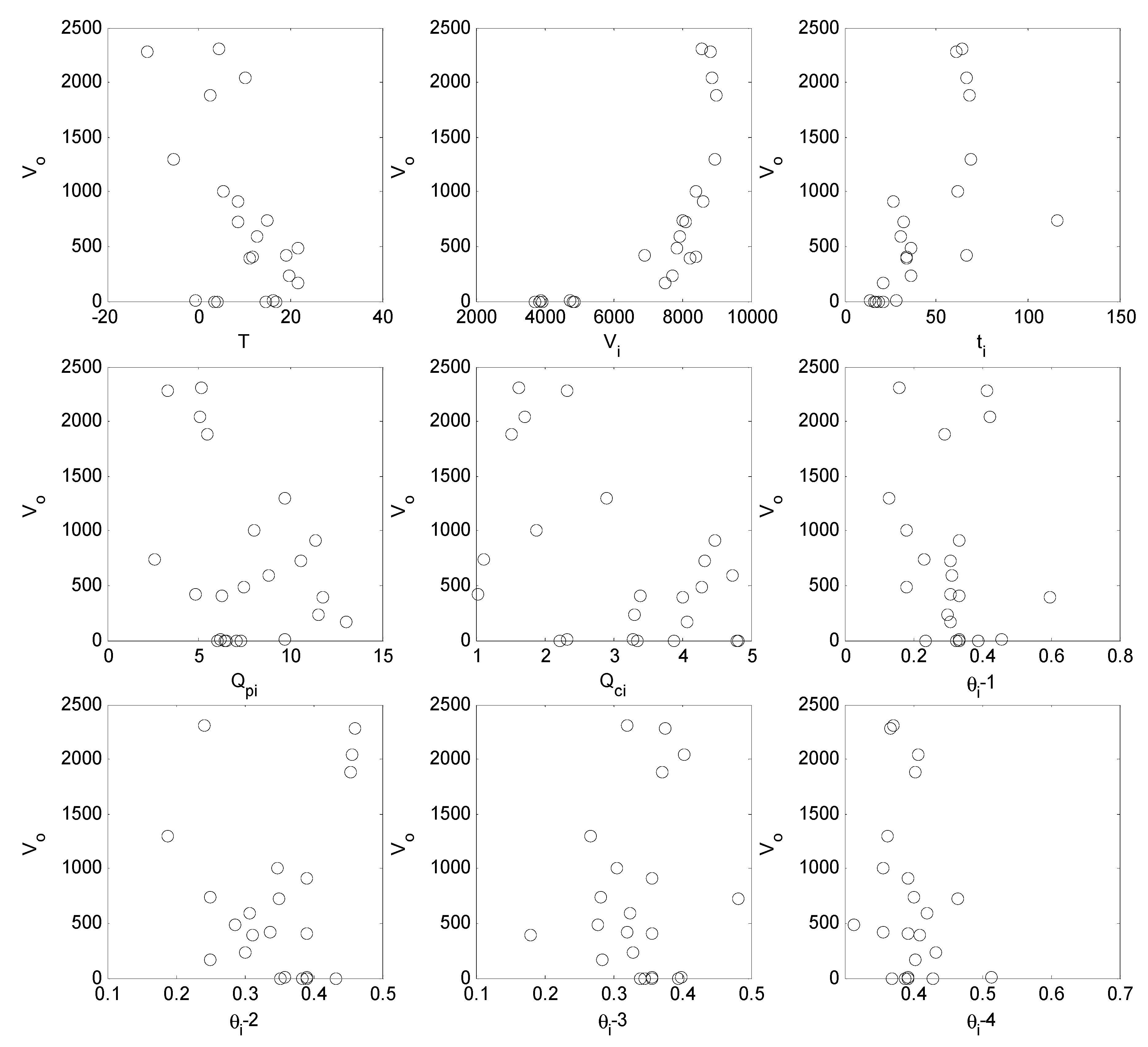
A correlation analysis was conducted to determine the associations between
Vo and the other nine parameters.
Figure 2 shows pair-by-pair scatter plots of
Vo and these parameters. The figure illustrates that a single parameter cannot be used to describe all the variance in
Vo. Correlation coefficients were calculated for each pair;
Vo was significantly (with a
p-value < 0.05) correlated with
Vi (Pearson’s correlation coefficient
r, was calculated to be 0.73) and
ti (
r = 0.64). Non-significant (with a
p-value > 0.05) correlation was found between
Vo and
θi-2 (the soil moisture measured 300 mm below the surface, with
r = 0.14). Based on this, the candidates for regressors for the MLR were reduced from the original nine to
Vi,
ti and
θi-2.
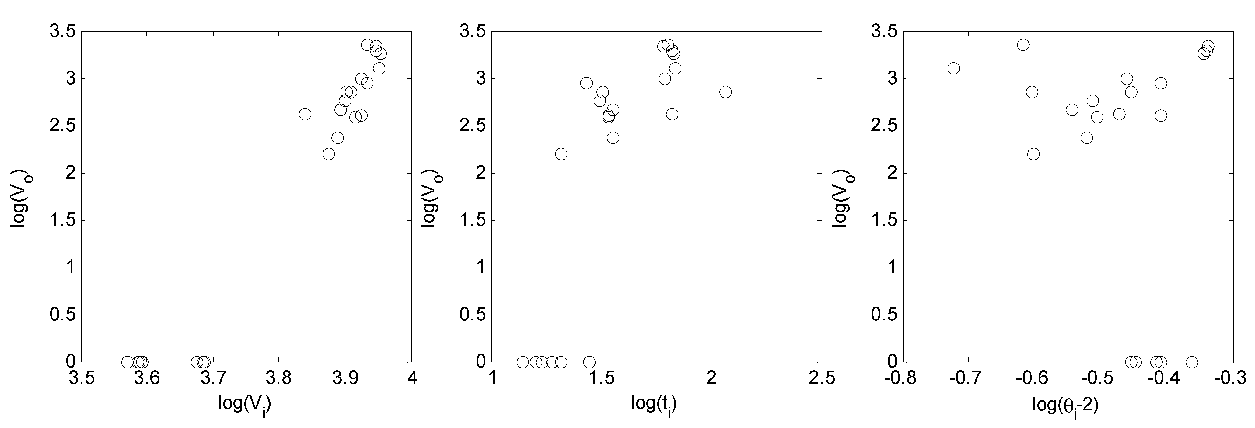
Figure 3 shows pair-by-pair scatter plots of these three parameters
versus Vo; in this figure the values plotted are the logarithm of the original observations. The linear correlation between these variables is clearer after the transformation. It should be noted that for events F3 to Sp1, Sp3 and S7 to S9,
Vo was less than 10 L (in fact,
Vo was equal to zero for five of the seven cases,
i.e., no effluent drained from the bioretention cell); these values were replaced with values of 1 L to facilitate the log-transformation. As such, experiments producing minimal effluent volume were considered to be of the same population (with the higher effluent volumes arising from a different population due to different generating mechanisms) with a very small variance. Thus, all effluent volumes less than 0.1% of the inlet volume, or 10 L, were assigned a value of 1 L.
Figure 2.
Pair by pair scatter plots of Vo and the nine independent variables.
Figure 2.
Pair by pair scatter plots of Vo and the nine independent variables.
Figure 3.
Pair by pair scatter plots of log-transformed Vo, the two significantly correlated variables, Vi, and ti, and weakly correlated θi-2.
Figure 3.
Pair by pair scatter plots of log-transformed Vo, the two significantly correlated variables, Vi, and ti, and weakly correlated θi-2.
4. Model Construction and Validation
After the candidate regressors to predict
Vo were identified, the data was divided for model construction and validation; 15 data points were used for model construction and 8 were used for validation. The data were split to ensure an equal representation of cold climate events in both sets as well as no significant deviation from the population mean.
Table 2 summarizes statistics of the original and the divided data, and identifies the experiment ID that corresponds to each data set.
Table 2.
Summary of statistics of all experiments, construction and validation data sets for the three regressor candidates and Vo.
Table 2.
Summary of statistics of all experiments, construction and validation data sets for the three regressor candidates and Vo.
| Statistic | Vi (L) | ti (min) | θi-2 (m3/m3) | Vo (L) |
|---|
| All experiments | | | | |
| Mean | 7034 | 42 | 0.347 | 691 |
| Standard Deviation | 1955 | 25 | 0.073 | 770 |
| Experiments used for construction: |
| S1, S2, S3, F3, W1, SP2, SP3, S5, S7, S9, F4, W2, W3, S11, S12 |
| Mean | 6893 | 44 | 0.371 | 673 |
| Standard Deviation | 2050 | 29 | 0.068 | 799 |
| Experiments used for validation: |
| S4, F1, F2, SP1, S6, S8, W4, W5 |
| Mean | 7299 | 38 | 0.303 | 724 |
| Standard Deviation | 1866 | 19 | 0.064 | 763 |
The construction data set was then used to construct six MLR models using Equation (2) with different combinations of the regressors. The models are summarized in
Table 3, which lists the regressors used and the values of regression coefficients for each. Based on the error statistics for both the construction and validation sets (summarized in
Table 3), Model 2 which used
Vi and
ti as the regressors, emerged as the best performing model. Model 2 outperformed the other models based on a collective evaluation of error statistics, rather than leading in a single category. An advantage of using Model 2 to predict bioretention performance is that these two variables are typically readily available from historical records, and thus can be easily used to predict bioretention cell performance, without the need for other detailed site characteristics (e.g., soil type or the degree of imperviousness in upstream catchment area).
Table 3.
Summary of six multiple linear regression (MLR) model results, including regressors, xi used, the constant term A, coefficients Bi, and error statistics for both model construction (top row) and model validation (bottom row).
Table 3.
Summary of six multiple linear regression (MLR) model results, including regressors, xi used, the constant term A, coefficients Bi, and error statistics for both model construction (top row) and model validation (bottom row).
| Model # | Input | A | B1 | B2 | B3 | R2 | RMSE | MAE | AICc |
|---|
| 1 | x1 | log(Vi) | −33.94 | 9.39 | - | - | 0.98 | 0.195 | 0.136 | −22.2 |
| 0.98 | 0.161 | 0.109 | −11.9 |
| 2 | x1 | log(Vi) | −30.60 | 8.14 | 0.91 | - | 0.99 | 0.128 | 0.086 | −28.5 |
| x2 | log(ti) | 0.98 | 0.178 | 0.145 | −11.1 |
| 3 | x1 | log(Vi) | −33.74 | 9.42 | 0.71 | - | 0.98 | 0.191 | 0.123 | −22.5 |
| x2 | log(θi-2) | 0.98 | 0.203 | 0.144 | −10.1 |
| 4 | x1 | log(Vi) | −30.34 | 8.16 | 0.93 | 0.77 | 0.99 | 0.120 | 0.079 | −29.5 |
| x2 | log(ti) |
| x3 | log(θi-2) | 0.97 | 0.221 | 0.164 | −9.41 |
| 5 | x1 | log(ti) | −4.46 | 4.08 | - | - | 0.58 | 0.901 | 0.616 | 0.744 |
| 0.68 | 0.721 | 0.553 | −0.050 |
| 6 | x1 | log(ti) | −4.25 | 4.09 | 0.53 | - | 0.59 | 0.888 | 0.600 | 0.526 |
| x2 | log(θi-2) | 0.65 | 0.754 | 0.600 | −0.408 |
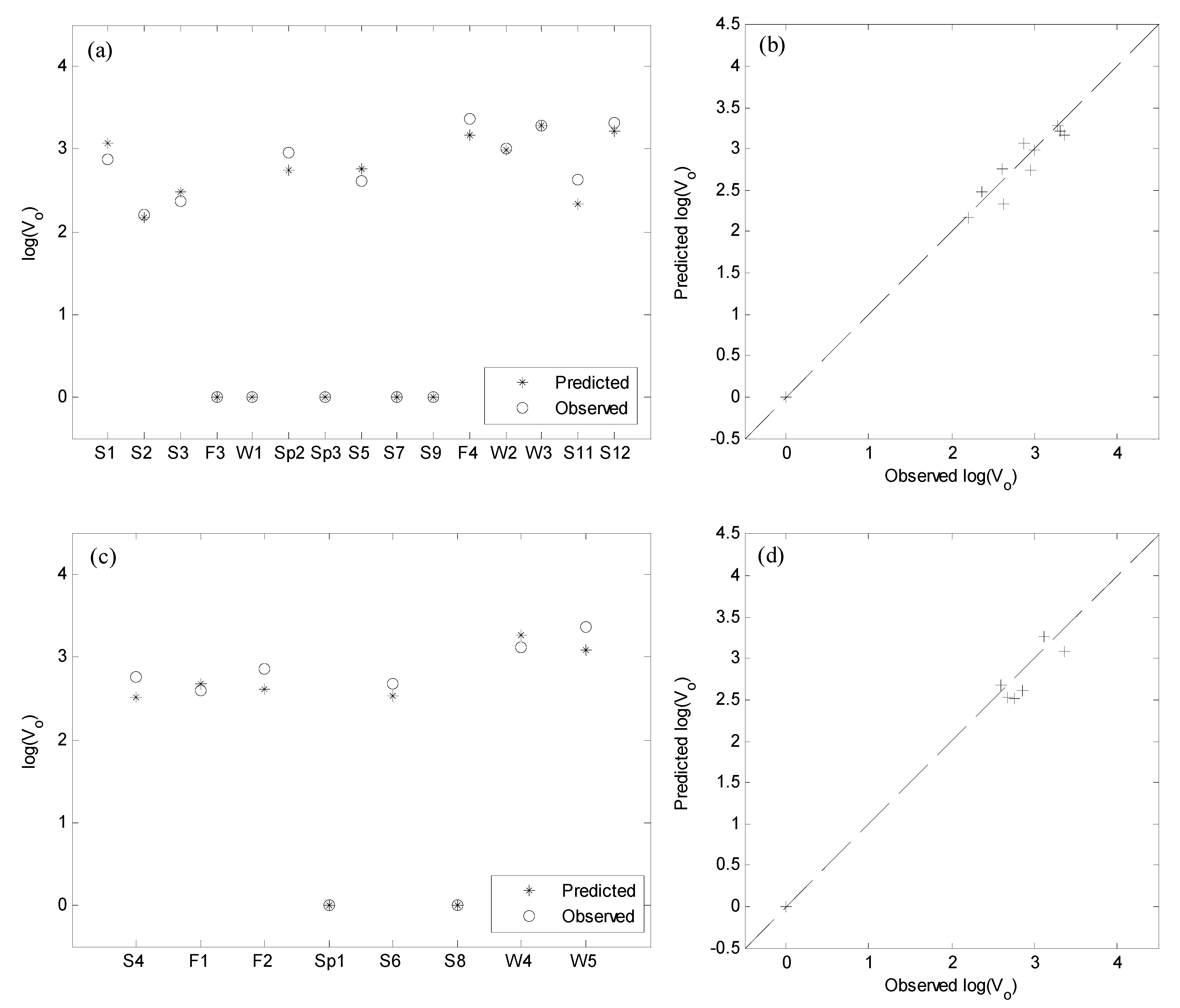
Figure 4 below shows a comparison of the observed and predicted data using Model 2. The figure shows that the model can accurately predict both the lower (~0 L) and higher end of the observed
Vo. It is important to note this model was designed so that predicted
Vo values between 0 L and 10 L were set equal to 1 L to be consistent with the rule used described in
Section 3. This assumes that predicted low effluent volumes (between 0 L and 10 L) are essentially the same population as the case when no runoff drains from the bioretention cell.
Figure 4 also shows that the observed and predicted values closely follow the 1:1 line, in both the construction and validation data sets.
The upper and lower limits of the input data for Model 2 are influenced by the data used to construct the model. Vi ranged from 3720 L to 9100 L, while ti ranged from 14 min to 116 min. The application of the model is approximately limited to these values. Furthermore, the limit of the predicted values of this model are bounded by Vo = 0 L (100% of inlet runoff captured) and by Vo ≤ Vi (maximum outlet runoff cannot be greater than inlet runoff). Therefore, it is important to ensure that the input variables used for prediction do not exceed the upper limits of Vi and ti.
Figure 4.
Model 2 results: time series comparison of observed and predicted log(Vo) for (a) construction, and (c) validation data sets; and comparison of predicted and observed data sets for (b) construction and (d) validation data sets.
Figure 4.
Model 2 results: time series comparison of observed and predicted log(Vo) for (a) construction, and (c) validation data sets; and comparison of predicted and observed data sets for (b) construction and (d) validation data sets.
5. Model Application
One of the objectives of this research was to use an MLR model to create a design tool to assist in designing bioretention cells, for region-specific applications. To do this, historical precipitation depth and duration data for Calgary were used to predict Vo using the developed model. An important intermediate step in this process is the conversion of the precipitation depth to Vi. A method that accounts for the size of a bioretention cell and the size and degree of imperviousness of its upstream catchment is used and described below.
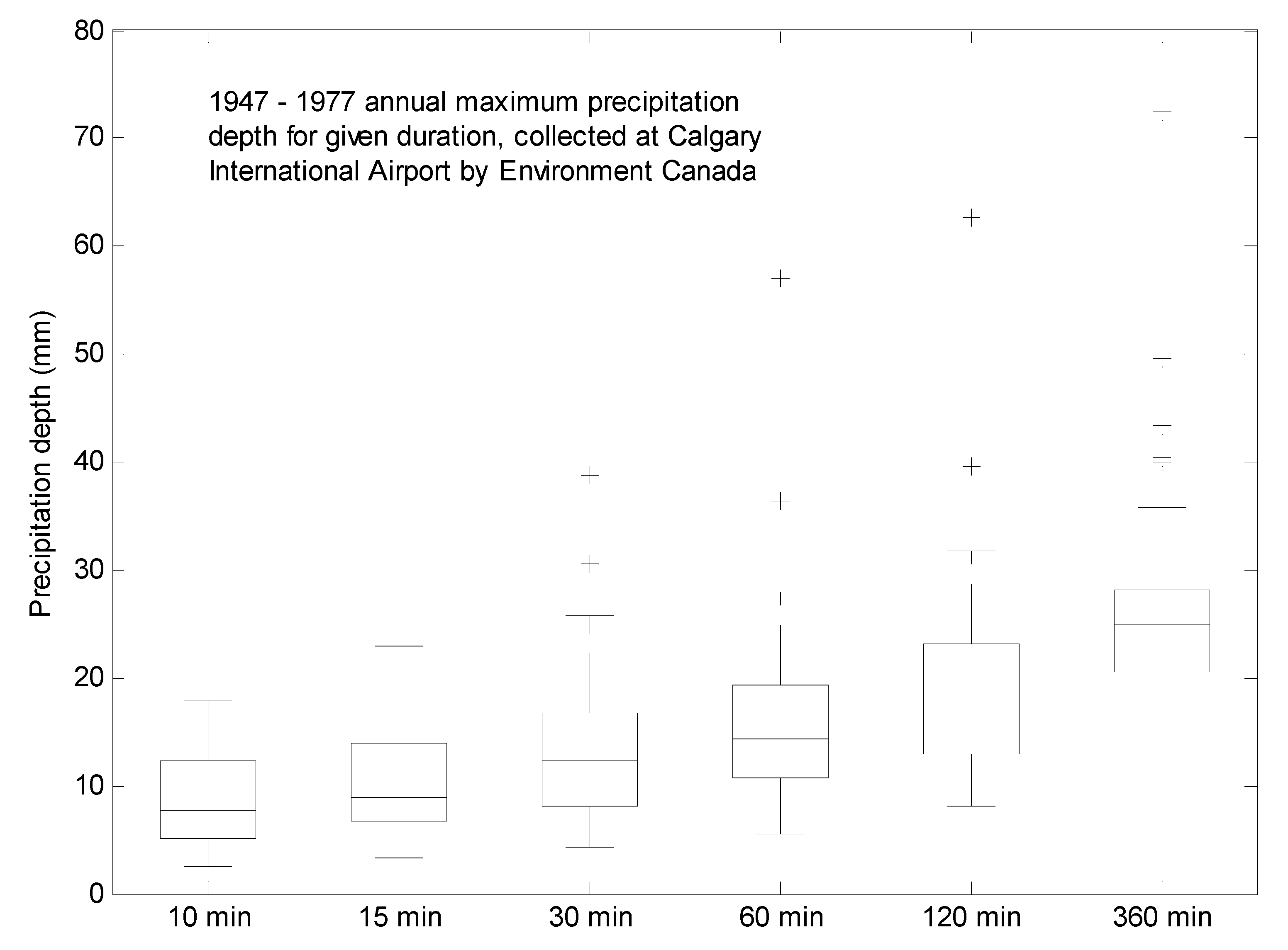
Historical precipitation and duration data was collected from Environment Canada [
23]. The data, part of the
Short Duration Rainfall Intensity-Duration-Frequency Data set, includes the maximum precipitation depth observed in Calgary (Calgary Int’l A, ID: 3031093) at nine event durations. The data from 1947 to 2007 (with six years data missing) includes event durations from 5 min to 24 h.
Figure 5 summarizes the maximum precipitation depths at each interval for the 60 year period. Note that events with a duration of less than 10 min and more than 6 h were excluded in the figure and in the proceeding analysis, as this data does not meet the criteria for the MLR model outlined in
Section 4.
Figure 5.
Summary of historical maximum precipitation depth and corresponding duration for Calgary, collected from Environment Canada for the years 1947–2007.
Figure 5.
Summary of historical maximum precipitation depth and corresponding duration for Calgary, collected from Environment Canada for the years 1947–2007.
The volume of runoff generated in a catchment from a given precipitation depth is a function of both the area and the degree of imperviousness of the catchment. Both these factors need to be included to calculate
Vi from the historical precipitation depths. First, the area of the catchment has to be defined; typical guidelines recommend that a bioretention cell should be sized from 5% to 20% of the catchment area [
24,
25]. For this research, four different catchment sizes were used, where bioretention cell area (which was equal to 32 m
2 for the experiments) was 5%, 10%, 15% and 20% of the total catchment area. The corresponding catchment areas are 160, 213.3, 320 and 640 m
2.
Second, the amount of impervious area of the catchment area has to be defined. A typical residential area in Calgary will have an impervious area of 40% whereas in commercial areas or parking lots it can be as high as 100% (i.e., 100% of the catchment has impervious surfaces). For the application of the MLR model, four different levels of impervious areas were used: 100%, 80%, 60% and 40%, representing typical catchment characteristics found in urban areas. For example, for a 320 m2 catchment, if the amount of impervious area in a catchment is 40%, the area of the impervious surfaces is 128 m2.
A ratio known as the Impervious to Pervious Ratio (
I/
P) was introduced [
15,
26].
I/
P is the ratio of the upstream impervious area (
I) to the area of the pervious bioretention cell (
P) that receives the runoff. Thus, continuing from the example above, the impervious fraction (
I) is 128 m
2, while the bioretention area (
i.e.,
P) is 32 m
2, meaning the
I/
P = 128 m
2/32 m
2 = 4. The
I/
P approach is useful since it can combine both factors: the total area, and the imperviousness of the catchment, into a single relationship which can be formulated as:
where
Vi = volume of influent (m
3);
d = precipitation depth (m);
AB = bioretention cell area (m
2); and
I/
P = Impervious to Pervious Ratio. Equation (7) takes into account the runoff generated from the impervious area in the catchment and also the precipitation that occurs on the bioretention cell itself. A summary of the
I/
P calculated for the 16 combinations of catchment size and impervious areas are shown below in
Table 4. Though Equation (7) shows that
Vi is a function of the area of bioretention cell,
AB, this is not explicitly necessary, and Equation (7) can be rewritten in a more general form as:
where
Aimp is the impervious area of the catchment (m
2);
PoC is the size of the bioretention cell as a percentage of the total area of the catchment, e.g., between 5% and 20% (%); and
AC is the area of the catchment that drains for the bioretention cell (m
2).
Table 4.
Summary of I/P values calculated for 16 different combinations of catchment size and percent impervious area in the catchment.
Table 4.
Summary of I/P values calculated for 16 different combinations of catchment size and percent impervious area in the catchment.
| Percent Impervious Area | Percentage of catchment size |
|---|
| 5% | 10% | 15% | 20% |
|---|
| 100% | 20 | 10 | 6.7 | 5 |
| 80% | 16 | 8 | 5.3 | 4 |
| 60% | 12 | 6 | 4 | 3 |
| 40% | 8 | 4 | 2.7 | 2 |
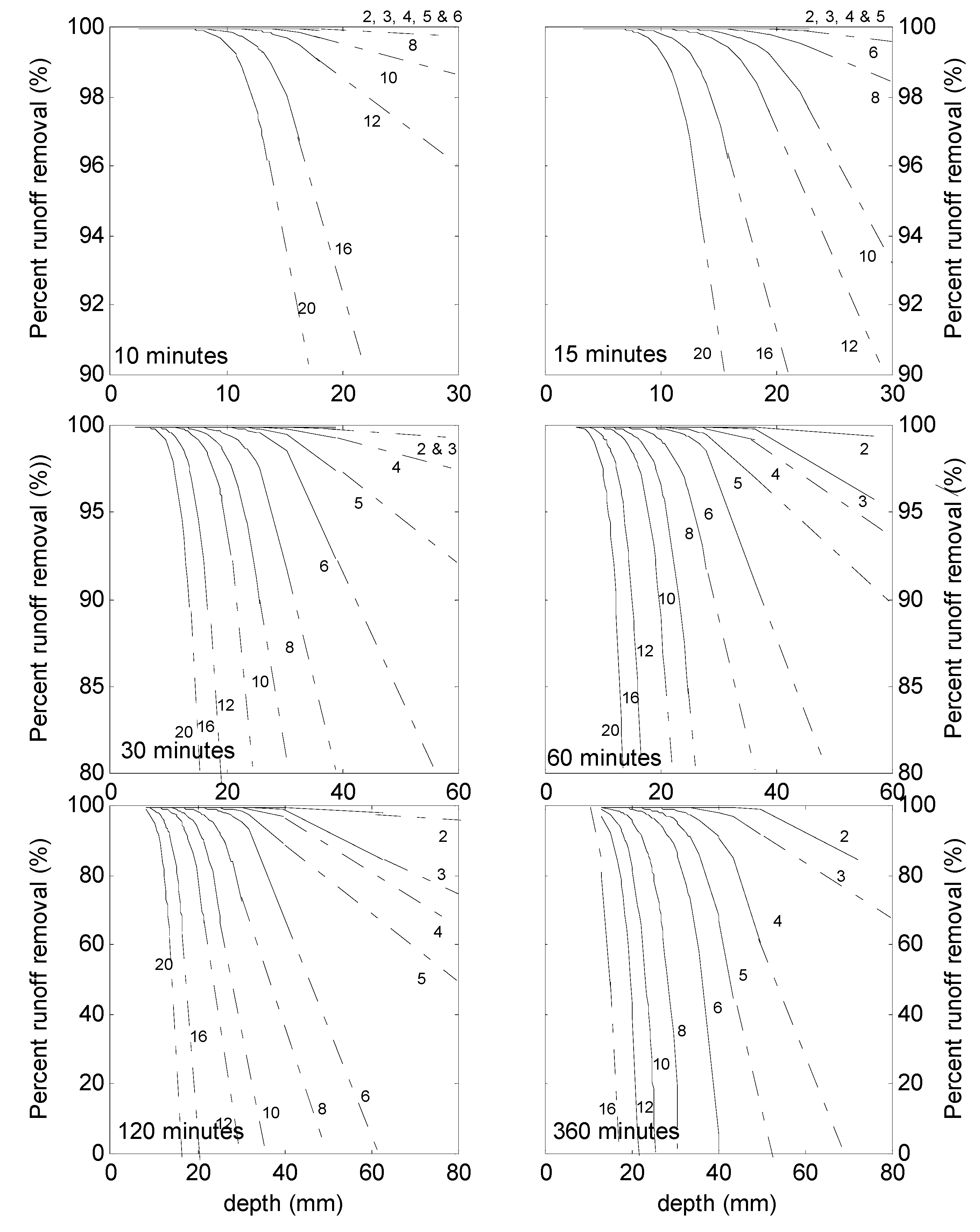
After the
I/
P values were determined,
Vi values were computed for the entire historical data set. Values of
Vi that exceeded 9,100 L were excluded from further analysis. These values were then used as input in Model 2. The resultant
Vo, determined from the model output, were used to calculate
ΔV using Equation (1). The results are plotted in
Figure 6 below. The figure shows predicted
ΔV values
versus the precipitation depth at six different duration intervals. Further, at each duration, the
ΔV values are further categorized by
I/
P values. The solid black lines represent predicted values calculated by the model, whereas the dashed lines are extrapolation of the predicted trends.
To illustrate the functionality of the figure, take the following examples: given an event with a duration of 60 min and depth of 30 mm, the expected ΔV, for a bioretention cell sized to an I/P of 8, is approximately 90%. Conversely, if ΔV is known a priori, for example development regulations stipulate that 80% of runoff must be captured, the figure can be used to determine the necessary I/P ratio. This ratio can be used to calculate the size of the bioretention cell needed, assuming that the total catchment size is known, to meet the performance goals, for a given “design event”. For example, to capture 80% of runoff generated from a 25 mm, 120 min event, the figure shows that the necessary I/P of the cell has to be 8 or lower. However, if the “design event” is, for example, 25 mm over 60 min, the I/P value can be up to 10 to meet the runoff reduction goals. This increase can be achieved by either decreasing the size of the bioretention cell, relative to the size of the catchment, or more impervious surfaces can be added to the catchment, or a combination of both.
These examples show how
Figure 6, which was developed using local experimental and historical data, can be used as a design tool to size bioretention cells for use in Calgary. Once the performance targets are known, different sizes can be explored using this figure, based on catchment characteristics and available area. Limitations of the tool include the maximum permissible
Vi, and also the characteristics of the experimental bioretention cell used to generate the data.
Figure 6.
Bioretention cell design guide for Calgary: runoff volume reduction as a function of precipitation depth, duration and I/P ratio.
Figure 6.
Bioretention cell design guide for Calgary: runoff volume reduction as a function of precipitation depth, duration and I/P ratio.
6. Conclusions
LID is a sustainable water management strategy that aims to integrate water management into the urban fabric. As a site design strategy, LID can be considered more than just a stormwater control technology; it is a tool that promotes a full spectrum of ecosystem benefits. LID, including bioretention cells, are an emerging technique of addressing urban stormwater management: techniques that move away from traditional practices of expanding urban infrastructure, to providing engineering answers at the lot-level.
Bioretention cells are a proven technology to address urban runoff concerns in cold climate conditions, like that of Calgary, Canada [
15,
22]. This paper developed a novel method to create a design tool to assist in bioretention design, for Calgary, that takes region-specific design considerations into account. Currently, no guidelines or models exist to design bioretention cells for use in Calgary. In this paper, experimental data was used to create a data-driven model to predict bioretention cell performance, specifically the amount of runoff captured. This research shows that the volume of runoff draining to a bioretention cell and the duration of a precipitation event can be successfully used to predict bioretention cell performance. The model performed well with respect to R
2 (0.991), RMSE (0.128), MAE (0.086) and AIC (−28.8). Historical precipitation depth and duration was then used to predict bioretention cell performance under 16 different catchment characteristics, including varied levels of imperviousness and catchment size. These results were collated and extrapolated to create a novel design tool, shown in
Figure 6. This figure was then used to demonstrate how future bioretention cell design size can be estimated if performance targets are known. An example also showed how bioretention cell performance can be estimated if the size and characteristics of the catchment are known. Though the methodology was applied to only one case study, Calgary, it can be applied in any region where the relevant data is available.
Future research should focus on advancing this technique by expanding the scope of performance parameters. Other hydrological performance parameters, such as peak flow reduction, are closely correlated with the decrease in runoff volume, and a data-driven technique may be applied to predict these parameters as well. Similarly, future work should focus on predicting water quality performance by using the hydrological performance as an indicator.


