A Heat Budget of the Mar Menor Lagoon, Spain

Abstract

The Mar Menor is the second largest coastal lagoon in the Mediterranean Sea, with a surface area of about 136 km². It is restricted from the open sea by a sandy barrier system (La Manga) interrupted by three tidal inlets. As a result of high evaporation, it is hypersaline (42–47 ppt) in parts. This study examines the factors leading to the rise in sea surface temperature in the Mar Menor through an analysis of long-term sea surface temperature using HadSST1.1 data together with shorter-term Moderate-Resolution Imaging Radiometer and Optimum Interpolation Sea Surface Temperature data. A thermal box model has been constructed for the lagoon in an attempt to balance major heat sources and sinks. Additionally, a thermal probe was deployed in 0.3 m of water to evaluate the benthic flux of heat of the shelly fine sand that covers the lagoon seabed. The results show that the vertical thermal gradient in the seabed inverts between the day and night. Prior to circa 1977, there was no clear trend in SST, and variations were strongly associated with the Atlantic Mutidecadal Oscillation and the North Atlantic Oscillation. Post circa 1980, the maximum summertime sea surface temperature showed a steady increase of 0.34 °C/decade. The cross-correlation of SST in the Mar Menor with external drivers showed that it is dominated by the sea surface temperature of the Western Mediterranean, followed by local air temperature, with a minor contribution from the Indian Ocean Dipole. No other significant correlations were evident, suggesting that local temperature was dominated by local drivers. In addition, a Spearman rank order evaluation and principal component analysis showed that the general trends of the Mar Menor SST were also influenced by the Atlantic Multidecadal Oscillation, CO₂, and GDP.

1. Introduction

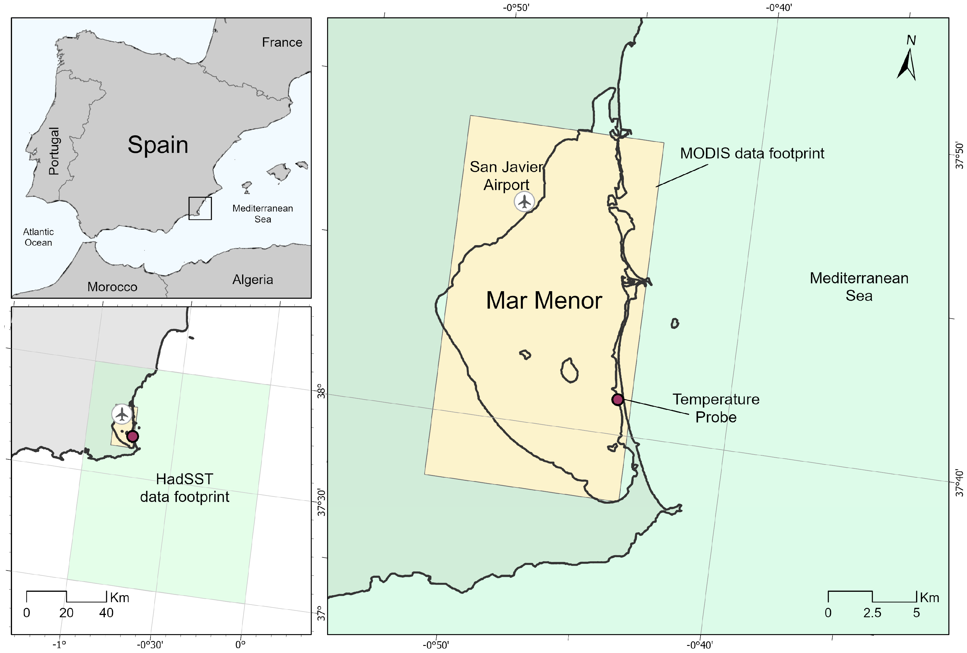
The Mar Menor, located in the southeast of Spain, is the second largest lagoon in the Mediterranean Sea with a surface area of about 136 km². It is restricted from the open sea by La Manga, a 22 km long sandy barrier crossed by three tidal inlets (Figure 1). As a result of an annual evaporation rate that is 3 to 4 times greater than rainfall, it is hypersaline (42–47 ppt) in parts [1,2], which gives the lagoon a unique environmental character such that it constitutes a refuge for some endemic species. Moreover, it contains 856 ha of fringing salt marsh that is used as a stop-over by migrating shore birds. As a result, it was designated a Ramsar wetland in 1994. It is shallow (a mean depth of 4.5 m) and has been highly impacted by “massive urban growth” [3]. Some sites are contaminated with heavy metals from old mining discharges [4,5], manifested as bio-accumulation (of Zn, Cd, and Pb) in bivalves and by the take-up of toxins by seagrass plants such as Cymodocea nodosa. The solubility and mobility of such toxic metals increase with water temperature [6]. This is particularly true in fine-grained sediment such as that of the southern Mar Menor. The increase in eutrophication and anoxia due to “unsuitable agricultural methods”, which introduce excess nitrates and phosphates into the system, has had significant impacts on the biosphere of the lagoon [7,8,9,10]. Groundwater discharges and flood events introduce nutrient loads from the catchment area. These events can produce algal blooms that significantly reduce the water oxygen content and can cause mass mortalities, as observed in recent years (2016, 2019 and 2021). Water temperature has been shown to be a major factor leading to enhanced eutrophication in aquatic settings, which, in combination with the two nutrients, has far reaching effects on biological community dynamics [11]. The bio-accumulation of toxins is also enhanced by the long residence time of waters (average of 0.79 years) [12,13].

A surface energy budget for a coastal lagoon (Nueva lagoon) in S.E. Spain was undertaken by [14], referred to hereafter as RR06. The formulation and structure of this budget were followed in the Mar Menor by [15], referred to hereafter as MA11, who asserted that there was limited information on the hydrodynamics of the system. More recently, 3-D numerical modeling of the hydrodynamics of the Mar Menor has significantly enhanced the understanding of the structure and dynamics of the lagoon under both tidal and wind-forced conditions [13]. Whilst temperature and salinity were imposed in a 3D hydrodynamic model (SHYFEM) open boundary [16], sources and sinks of heat within the system were not included. This paper attempts to provide a simple heat box model of the Mar Menor that includes all major local sources and sinks of heat following the structure defined in the previously quoted papers. The exchange of heat across the benthic boundary layer is rarely included in models due to a lack of information on the thermal properties of the bottom sediments (a notable exception is RR06). Part of this work is to measure the temperature gradient in the topmost 0.45 m of the seabed in order to determine the heat exchange (in W/m²) of the seabed with the waters of the Mar Menor, which may provide useful input for advanced hydrodynamic models such as SHYFEM.

The Mar Menor is dominated by sandy sediments in shallow regions and mud in deeper parts. The distribution, character and dynamics of such sediments can be greatly impacted by changes in water temperature, as can benthic exchanges with the water column, which impact turbidity and water clarity [10,17,18]. Seasonal fluctuations in the sea surface temperature (SST) in the Mar Menor are of the order 21 °C (10–31 °C) largely due to the shallow water depths [9]. These fluctuations are higher than those in the open sea. The seasonal effects of SST on the biological productivity of coastal lagoons can be large [19], as is the impact of dredging the channels connecting Mar Menor with the open sea [13]. Furthermore, the SST of coastal lagoons has been increasing at a faster rate than the global average [20,21,22]. The SST in the Venice lagoon, for example, has been increasing at a rate of up to 1.75 °C/decade since 2008 [21]. It is not unreasonable to expect that the temperature trend in Mar Menor will be greater than is the case for the Venice lagoon, as the flushing of warm water with the open sea results in a residence time of up to 1 year [13].

Thermal probe measurements have been made in order to examine the benthic exchanges of heat (an open boundary usually omitted from heat budgets), which have not been done before in the Mar Menor. A detailed analysis of the air and SST trends in the Mar Menor updated for 2024 is used to examine the external drivers of thermal trends. The work presented herein aims to determine the SST trends of the Mar Menor and the factors that influence these trends as a basis for enhanced forecasting and prediction systems and as boundary conditions for ocean, weather and seasonal modeling [23].

2. Materials and Methods

The factors influencing the hydrology and hydrodynamics of the Mar Menor have been defined by [2]; their definition of inputs and losses to the system has been used as a guide herein. In particular, the gross annual budgets of surface runoff, seawater exchanges at the inlets, ground water discharge, and evaporation are taken from this source. Other sources of information are defined below.

2.1. Thermal Probes

Hourly measurements of the temperature were made by four self-logging thermistors (Signatrol^® SL52T, Signatrol, Tewkesbury, UK) installed in a thermal probe that was driven into the seabed in 0.3 m of water at low tide within the shallow subtidal region of the barrier Island at Playa de Galan (Lat: 37.685° N, Lon: 0.737° W, see Figure 1). The thermistors were factory calibrated to an accuracy of ±0.1 °C. Each thermistor was capable of logging temperature data hourly for about 5 months (3600 data points). Thermistors were located at a height of 0.15 m above the seabed, and at depths (h) of 0.15, 0.30 and 0.45 m below the seabed. Each thermistor was pre-programmed with date/time, and the data were downloaded to ASCII-format files using company software. The mean heat flux (q_z) was estimated from the temperature gradients using Fourier’s law:

$$q_z= -k{\displaystyle \frac{\mathsf{\partial }T}{\mathsf{\partial }z}} \mathrm{W}/{\mathrm{m}}^2$$

(1)

where ĸ is the thermal conductivity of saturated shelly sand (assumed as 1.5 W/m.K after [24]). Thermal diffusivity (α) is related to thermal conductivity as follows:

$$\alpha = {\displaystyle \frac{k}{\rho C_p}} {\mathrm{m}}^2/\mathrm{s}$$

(2)

where $\rho$ is the saturated bed sediment bulk density of the local well-sorted fine sand (d₅₀ = 0.23 mm) and is assumed as 1700 kg/m³, and C_p is the specific heat capacity (assumed to be 2.4 MJ/m³.K). Estimates of the temperature gradients (both during the day and night) are determined by defining the peaks and troughs of each temperature time series (that fluctuate daily). First-order polynomial best fits for the peak and trough temperatures were made to define daytime and nighttime values of ${\displaystyle \frac{\mathsf{\delta }T}{\mathsf{\delta }z}}$. It is assumed that the peaks and troughs in temperature are coincident in time and that the properties of the bed are constant with depth. Thermal diffusivity may also be estimated from

$$\alpha ={\displaystyle \frac{{∆z}^2}{2\ast lag}} {\mathrm{m}}^2/\mathrm{s}$$

(3)

where Δz = 0.45 m, and the lag is the time difference between the upper and lower peaks (in seconds).

2.2. The Mean Monthly Time Series Data

Mean monthly SST were downloaded from global sea surface temperature data sets (HadSST1.1) compiled by the Met Office, Hadley Centre (https://www.metoffice.gov.uk/hadobs/hadisst/ (accessed on 11 February 2020); [25]). A sub-set of the Western Mediterranean Sea (lat: 37–38° N; lon: 0–1° W, see Figure 1) was extracted using purpose-written code. SSTs for the Mar Menor were downloaded from MODIS Aqua (11 microns, night only, 4 km resolution) using the Giovanni tool (https://oceancolor.gsfc.nasa.gov/resources/giovanni/ (accessed on 12 March 2024)) available from July 2002 to the present (lat: 0.854–0.729° W; lon: 37.633–37.819° N, see Figure 1). It was shown that MODIS SST data were highly correlated with measurements in the Mediterranean Sea [26]. SST data for Mar Menor prior to 2002 were backfilled to September 1981 using the OISST blended analysis from NOAA (https://psl.noaa.gov/mddb2/makePlot.html?variableID=156646 (accessed on 12 March 2024); lat: 37.25–37.5° N; lon: 0–1° W). El Niño Southern Oscillation SST anomalies based on HadISST data (ENSO3.4, https://psl.noaa.gov/gcos_wgsp/Timeseries (accessed on 12 March 2024)) (in units of degrees Celsius) were downloaded from January 1870 to May 2024.

Mean monthly air temperature, wind speed, rainfall and cloud cover measured at San Javier airport (see Figure 1) were provided by AEMET (Agencia Estatal de Meteorologia) for the period 1950–2024. The major ocean oscillations were downloaded as follows: the Atlantic Multidecadal Oscillation (AMO, https://psl.noaa.gov/data/timeseries/AMO/ (accessed on 12 March 2024)); the Pacific Decadal Oscillation (PDO, https://www.ncei.noaa.gov/access/monitoring/pdo/ (accessed on 12 March 2024)); the North Atlantic Oscillation (NAO, https://www.ncei.noaa.gov/access/monitoring/nao/ (accessed on 12 March 2024)); and the Indian Ocean Dipole (IOD, https://www.cpc.ncep.noaa.gov/products/international/ocean_monitoring (accessed on 12 March 2024)).

The gross domestic product (GDP) for Spain was digitized from data provided by World Bank Group (https://data.worldbank.org/indicator (accessed on 12 March 2024)). Sunspot activity was provided by the World Data Center (WDC) Sunspot Index and Long-term Solar Observatory (SILSO) at the Royal Observatory of Belgium, Brussels (DOI: doi.org/10.24414/qnza-ac80).

2.3. Statistical Analyses

The HadISST1.1 global monthly time series was analyzed using purpose-written Matlab^® (2019b) codes. Data from January 1900 to December 2024 were examined in detail for this study. A 13-point moving average was applied to all time series to remove seasonality. The results were subtracted from the raw data to derive the seasonal components. A 13-term Henderson filter was applied to the raw data, and the results were compared to the filtered time series [27]. The long-term trends of the de-seasoned data were derived through a least-square linear best fit regression. A time series analysis of each calendar month was also undertaken following [28], and a least-square trend analysis was applied. The level of significance of the trends was examined in Sigmaplot^® (version 16), and the associated level of significance was estimated. SST anomalies (Had-SST-a, MM-SST-a) as defined by [29] were used in statistical analyses, which were defined as the de-seasoned value minus the long-term mean. The same procedure was applied to air temperature anomalies (MM-air-a) and CO₂ anomalies (CO₂-a) to provide de-seasoned time series that were comparable with the oceanic indices listed above.

Mean monthly data (MM-SST-a, “the dependent variable”; NAO, ENSO3,4, IOD, AMO, PDO, CO₂-a, sunspot number, GDP, and MM-air-a, “the independent variables”) for the period 1980–2024 (inclusive) have been analyzed through cross-correlation (to examine phase relationships) using Spearman rank correlation (non-parametric analysis less influenced by outliers) and using principal component analyses (PCA) in order to understand which rank order of factors appear dominant to explain the trends of air temperature and SST. PCA tests are valuable in examining which tested parameters participate together (modes) in explaining data variance. Cross-correlation is a complement to PCA and examines how variables relate in phase. Cross-correlation of MM-SST-a and MM-air-a was evaluated against the variables defined above and was carried out in Matlab^®; other statistical tests were undertaken in Sigmaplot^®. Satellite-derived SST can be 0.2 °K different from the waters below and may also be influenced by dust in the atmosphere [23]. These effects have not been considered in this study.

2.4. A Box Model for the Mar Menor

A box model of energy inputs and outputs to the Mar Menor seawater has been constructed following the work of [15] in order to assess the short term (months to years) drivers of SST. The purpose of the box model is to quantify (and balance) the sources and sinks of energy that result in the observed SST and to compare these results (at monthly time steps over 23 years, 2002 to 2024 inclusive) to the daily time steps (over 3 years) in [15]. A second purpose was to see if there were any fundamental changes in the heat balance that could be detected over the simulated period. Six main sources/sinks are recognized herein following [30]: (1) sensible heat exchanges between the air, ground, and seawater; (2) latent heat exchanges with the atmosphere due to evaporation; (3) incoming short- and long-wave solar radiation (modified by cloud cover); (4) outgoing long-wave radiation (also modified by cloud cover); (5) seawater/ground exchanges in sensible heat; and (6) tidal mixing/advection across the inlets. The sources/sinks of 1 to 4 are described in full by [31,32], together with relevant constants and coefficients. Tidal mixing across the inlets is described by [13].

The sensible heat flux (Q_air) from air to seawater is dependent on the mean temperature gradient between the air and water and the wind speed over water. It is defined as follows:

$$Q_{air}= {\rho }_{air}\times {Cp}_{air}\times C_h\times {xU}_{10}\times (T_{sea}-T_{air}) \mathrm{W}/{\mathrm{m}}^2$$

(4)

where ρ_air is the air density (1.22 kg/m³), Cp_air is the specific heat of air (1006 J/kg.C), C_h is the bulk transfer coefficient (1.2 × 10⁻³), U₁₀ is the wind speed (m/s) at a height of 10 m, x is an empirical coefficient (wind reduction factor) used to equate predicted (1.29 m/annum) and measured evaporation rates (1.35 m/annum, [2,15]), and T_sea and T_air are the mean monthly seawater and air temperatures, respectively.

SST in Mar Menor is also modified by the latent heat exchange due to evaporation (Q_lt), which, according to [32], requires information on the saturation-specific humidity (e_sat) and saturation air vapor pressure (q_sat):

$$Q_{lt}= l_v\ast C_e\ast C_h\ast {xU}_{10}\ast (q_{sat}-q_{air}) \mathrm{W}/{\mathrm{m}}^2$$

(5)

where l_v is the latent heat of vaporization (2.45 × 10⁶ J/kg at 20 °C and 42 psu) and C_e is the evaporation coefficient (1.5 × 10⁻³), and where

$$q_{sat}=0.622\ast {\displaystyle \frac{e_{sat}}{P-0.378\ast e_{sat}}}$$

(6)

where P is the atmospheric pressure (assumed as 1013 millibars or hectopascals) and

$$e_{sat}=6.112\ast \left({\displaystyle \frac{e^{\left(17.67\ast T_{air}\right)}}{{(T}_{air}+273.5)}}\right)$$

(7)

The effect of changes in salinity on the evaporation rate has been ignored.

Incoming top-of-the-atmosphere total solar radiation (Q_insol) is read from a mean monthly file (https://asdc.larc.nasa.gov/project/CERES/CERES_EBAF_Edition4.1 (accessed on 12 March 2024)). The incoming short- and long-wave radiation (Q_sol) is calculated as

$$Q_{sol}=Q_{insol}\ast \left(1-{\alpha }_s\right)\ast \left(1-0.7n_c\right) \mathrm{W}/\mathrm{m}$$

(8)

where α_s is the surface albedo of semi-arid terrains, such as those surrounding the Mar Menor (≈0.25), and n_c is the cloud cover fraction [31]. For present purposes, a long-term monthly average of cloud cover has been used (https://gmao.gsfc.nasa.gov/reanalysis/merra-2/ (accessed on 12 March 2024)).

Outgoing long-wave radiation (Q_out) is derived using the modified Stefan–Bolzmann relationship:

$$Q_{out}= \in \ast \sigma \ast {\left(T_{sea}+273.5\right)}^4\ast \left(0.39-0.05{q_{sat}}^{0.5}\right)\ast 0.19\left(1-0.01{n_c}^2\right) \mathrm{W}/{\mathrm{m}}^2$$

(9)

where ϵ is the emissivity of seawater (0.98), and σ is the Stefan–Bolzmann constant (5.67 × 10⁻⁸ W/m²/K⁴) where (K = T_sea + 273.5 °C) is the absolute water temperature. The modification to EQ 9 has been proposed by [33]. This formulation assumes cloud cover influence as defined above and was recommended for inclusion by [23].

The input of heat from rivers has been evaluated based upon annual discharge data from [2]. River water temperature is equated with air temperature. This fluvial input is defined as

$$Q_r={\displaystyle \frac{{\rho }_{water}\ast {Cp}_{fresh}\ast C_h\ast V\ast (T_r-T_{sea})}{Dt\ast A_{gr}}} \mathrm{W}/{\mathrm{m}}^2$$

(10)

where V is the mean monthly volume discharge of fresh water (m³), T_r is the mean monthly river water temperature, the time step Dt = 2630016 s (i.e., one month), Cp_fresh is the specific heat of fresh water (4180 J/kg.°C) and A_gr is the assumed surface area of the Mar Menor (1.36 × 10⁸ m²). A similar formulation to EQ 10 has been included to account for the rainfall measured monthly by AEMET (Q_rain), for the groundwater inflow (Q_gr), and for seawater exchanges across the tidal channels (Q_ch) [2].

The energy balance is then calculated following [14,15,31] as

$$Q_{bal}=Q_{sol}+Q_{air}+Q_{ch}+Q_{gr}+Q_r+Q_{rain}+Q_{out}+Q_{lt} \mathrm{W}/{\mathrm{m}}^2$$

(11)

The temperature change in SST (dT) is evaluated at monthly increments of time (per m²); the affected water mass (M_water) is estimated using a mixing depth (h) of 4.5 m [3] and is defined per unit area as

$$dT={\displaystyle \frac{Q_{bal}}{M_{water}\ast {Cp}_{water}}} °\mathrm{C}$$

(12)

where the unit water mass is

$$M_{water}={\rho }_{water}\ast h \mathrm{kg}.$$

(13)

The evaporation rate (E_v, m/month) is predicted as a function of the wind speed and relative humidity:

$$E_v= {\displaystyle \frac{C_e\ast x{U}_{10}\ast (q_{sat}-q_{air})}{{\rho }_{water}}}\ast dt \mathrm{m}/\mathrm{month}$$

(14)

Annual evaporation is estimated by summing the monthly evaporation depths. U₁₀ (wind speed at a height of 10 m) has been optimized in order to equate EQ 14 to the annual evaporation in the Mar Menor. This results in a wind reduction factor (x) of 1.0. This factor was initially used in EQs 4, 5 and 14 and then adjusted to balance EQ 11. Finally, the Bowen ratio (BR, the ratio of sensible to latent heat exchanges with the sea surface) was also estimated at monthly intervals.

3. Results

A stepwise approach to the SST in the Mar Menor was used to examine the heat budget post 1980. Firstly, the temperature profile measurements in the seabed are presented (in order to define seawater/seabed heat exchange relationships), followed by the Spearman rank order statistical analyses, then the cross-correlation of factors defined above to examine the phase relationships of factors, and finally the balancing of the heat budget within a box model. The results are compared to the output from [14,15].

3.1. Sea Surface Temperature

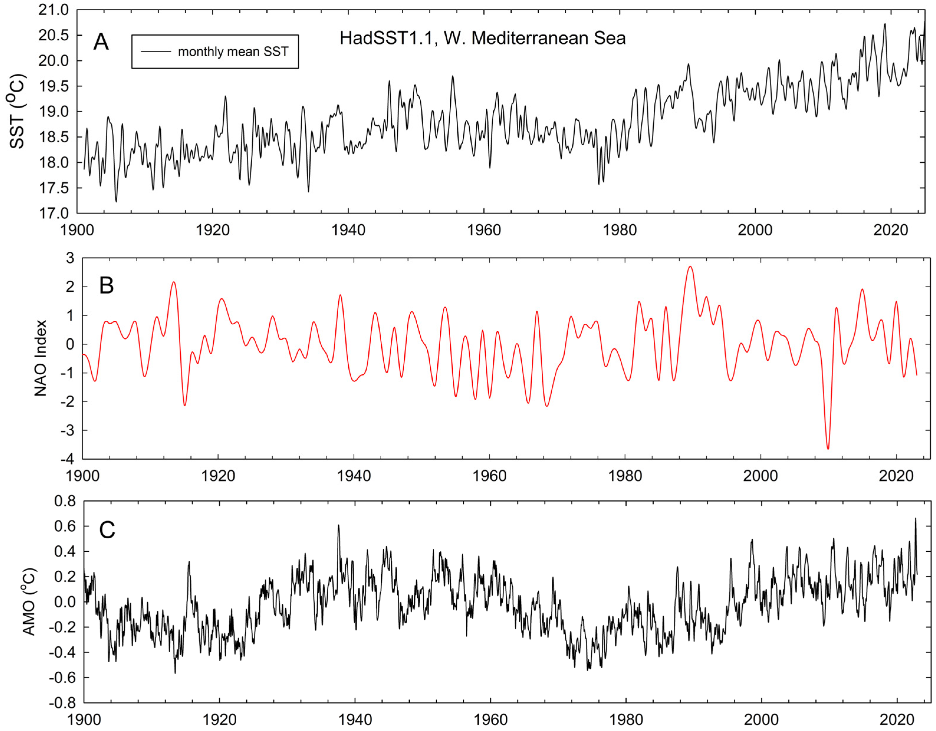
The Western Mediterranean is the open boundary for the Mar Menor and hence is an important influence on the heat budget of the lagoon. Monthly mean SST data from the W. Mediterranean Sea, extracted from the HadSST1.1 global data set, are presented from 1900 to 2024 (inclusive) in Figure 2A. Note that there is no clear trend in SST prior to circa 1977. Thereafter, there appears to be a systematic warming trend. It also appears that long-term variations in SST follow trends in the AMO (Figure 2C), while shorter-term peaks and troughs appear to follow those of the NAO (Figure 2B), as suggested by [26].

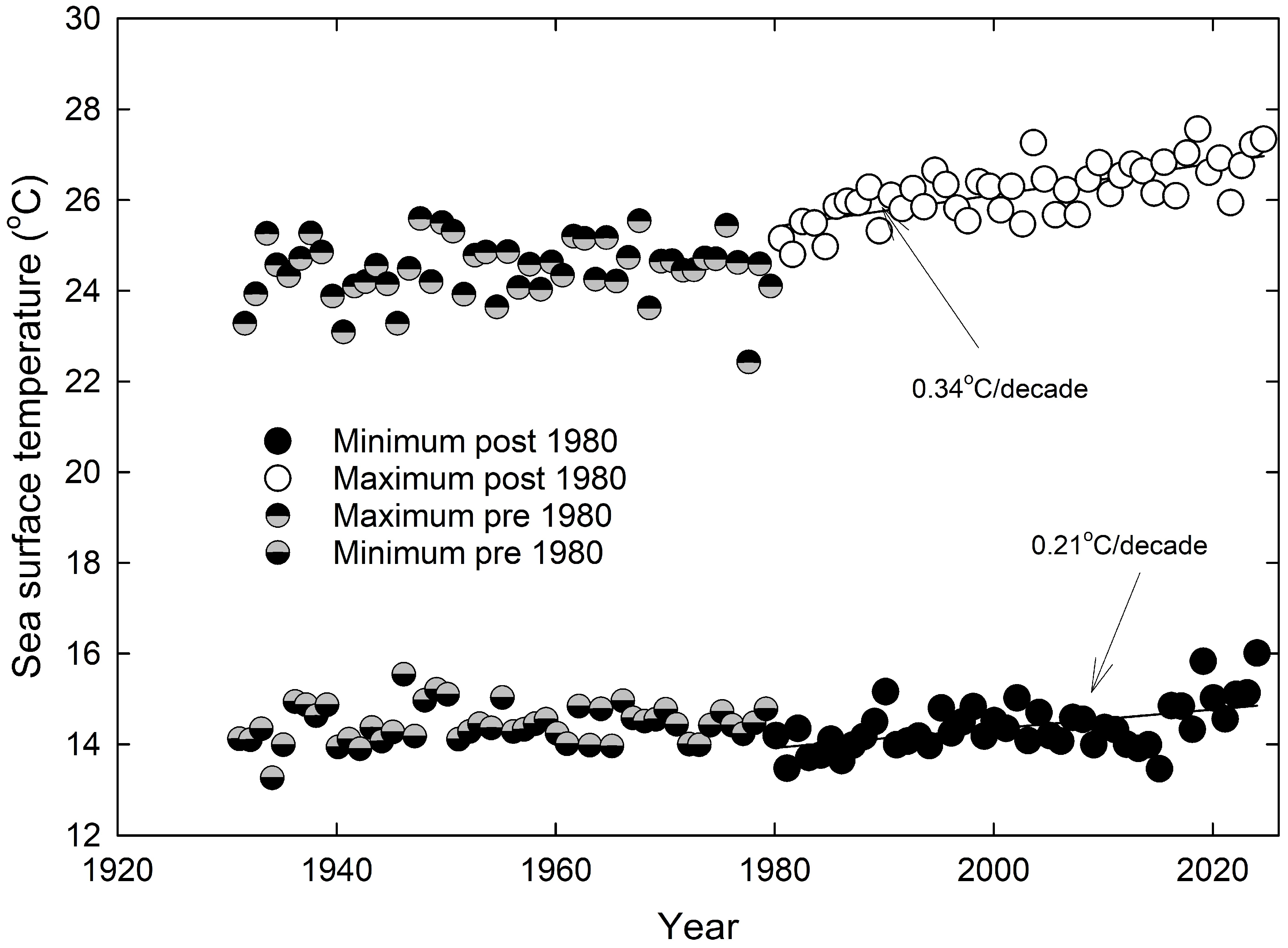
The annual maxima and minima in the SST of the Western Mediterranean (Figure 3) clearly show no trend for either extreme prior to circa 1980. Furthermore, the extremes appear remarkably consistent in time. Summer warming since 1980 shows a significant trend of 0.34 °C/decade (r² = 0.52, p < 0.001), as well as reduced scatter; the winter minima also show significant warming but at a lower rate of 0.21 °C/decade (r² = 0.26, p < 0.001). Refs. [34,35,36] have shown similar warming in their data analyses, which cover the period since 1979. Ref. [26] showed a stable increase in SST of 0.55 °C/decade for the period 2005–2019, which is manifested as a rapid rise in the minimum SST during this period.

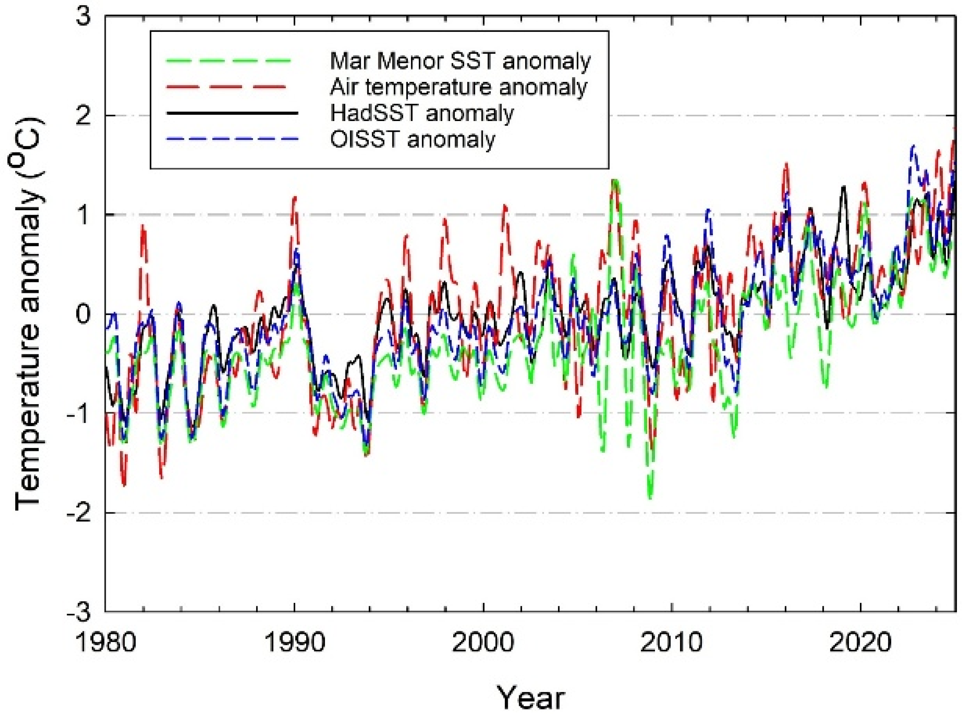
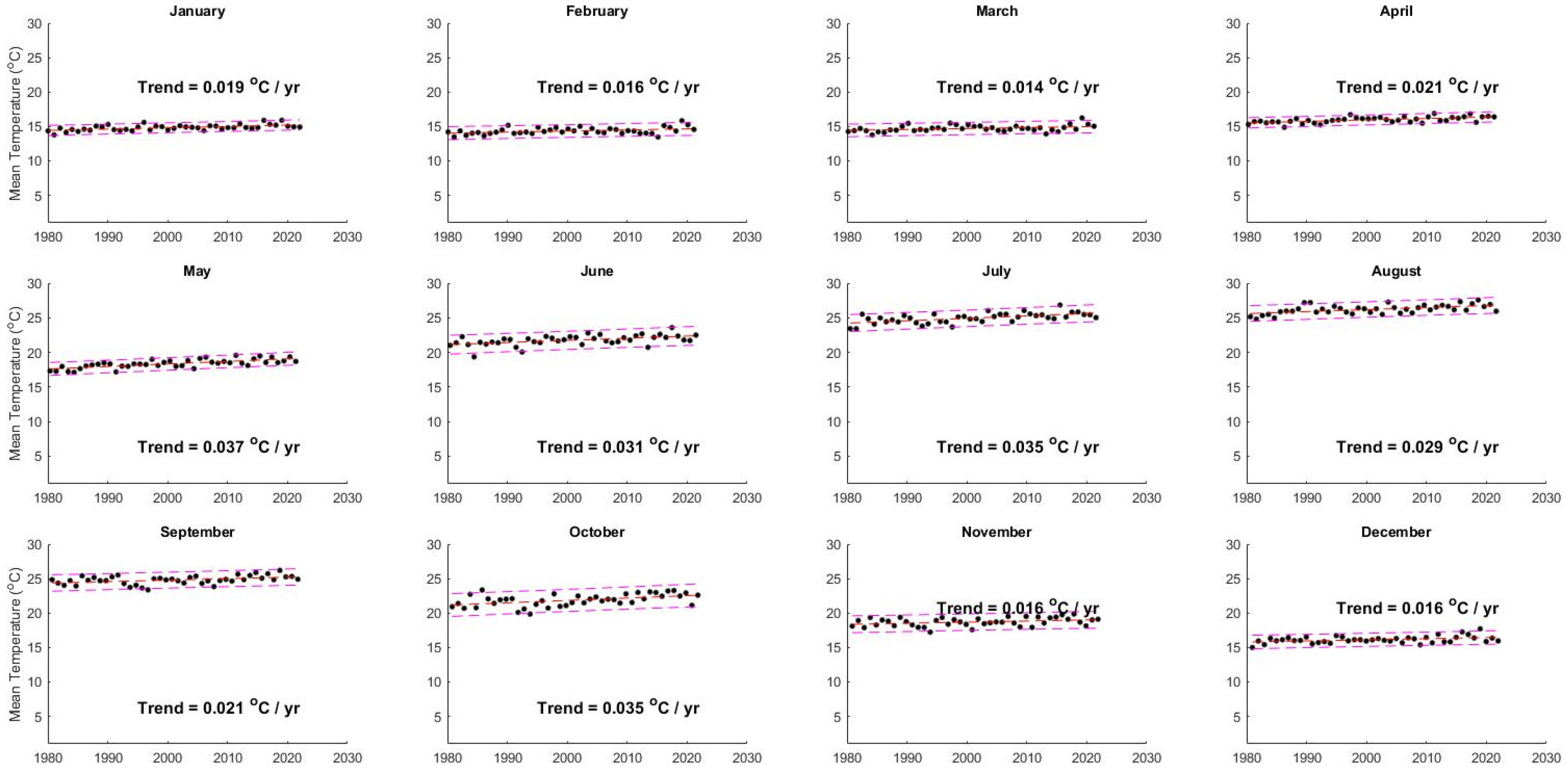
The SST anomalies post 1980 for the Western Mediterranean, the Mar Menor (MODIS), and the OISST (NOAA), together with the air temperature anomalies (MM-air-a) for the Mar Menor, are presented in Figure 4. Note that the peaks and troughs are generally consistent between records, though the Mar Menor is generally cooler than either the local air temperature or SST further offshore. Clearly evident in all data sets is the relative cooling presumed due to the volcanic explosions of Mount Pinatubo (1991–1994) and Hunga Tonga in January 2022 [37]. It is unclear if this is due to the changing sensitivity of the satellite sensor due to atmospheric dimming [23] or if this is a real change in SST. The least-square best fit trends in SST are presented for each month of the year in Figure 5. These trends are also listed in

Table 1. Least-square best fits of the temperature trends between 1980 and 2024 (inclusive) for (1) the W. Mediterranean (Had-SST); (2) Mar Menor SST (MM-SST), and (3) air temperature measured at San Javier airport (MM-air, see Figure 1). Almost all trends show significant warming. The Mar Menor appears to be warming at about twice the rate of the W. Mediterranean for most months of the year (low significance) and closely follows the warming of air temperature (high significance). The intensity of color is added for clarity and is proportional to the trends.

Source	Jan	Feb	Mar	April	May	June	July	Aug	Sept	Oct	Nov	Dec
Had-SST (°C/decade)	0.19	0.16	0.14	0.21	0.37	0.31	0.35	0.29	0.21	0.35	0.16	0.16
p-value	0.05	0.01	0.017	<0.0001	<0.0001	0.0005	<0.0001	0.0001	0.005	0.001	0.037	0.009
MM-SST (°C/decade)	0.67	0.32	0.38	0.41	0.04	0.36	0.62	0.48	0.59	0.73	0.63	0.41
p-value	0.034	0.25	0.17	0.28	0.98	0.22	0.007	0.11	0.11	0.06	0.041	0.055
MM-air (°C/decade)	0.16	0.12	0.27	0.49	0.6	0.52	0.61	0.56	0.36	0.42	0.21	0.13
p-value	0.13	0.29	0.006	0.0001	<0.0001	<0.0001	<0.0001	<0.0001	0.0002	<0.0001	0.048	0.22

. Notice that all months of the year show significant warming, with warming greatest in the summer and lowest in the winter.

3.2. Seawater to Seabed Heat Exchanges in the Mar Menor

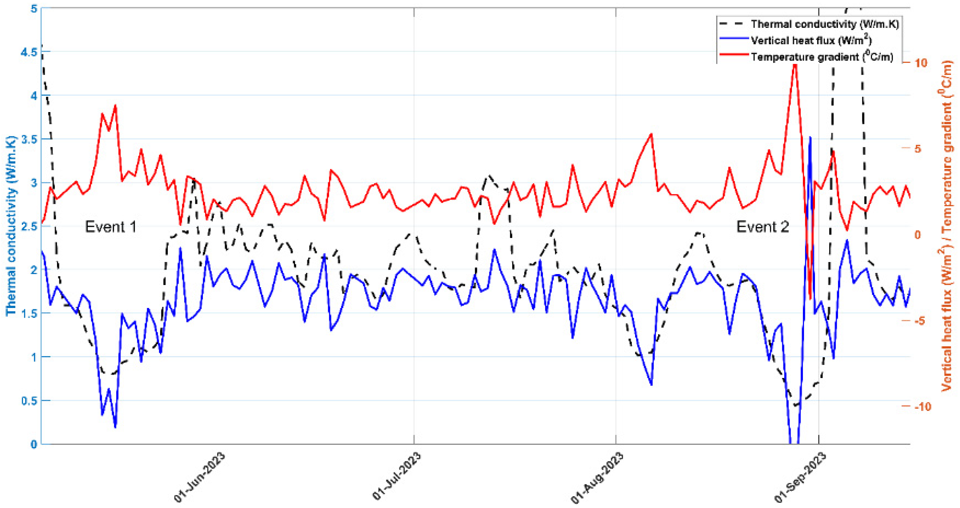
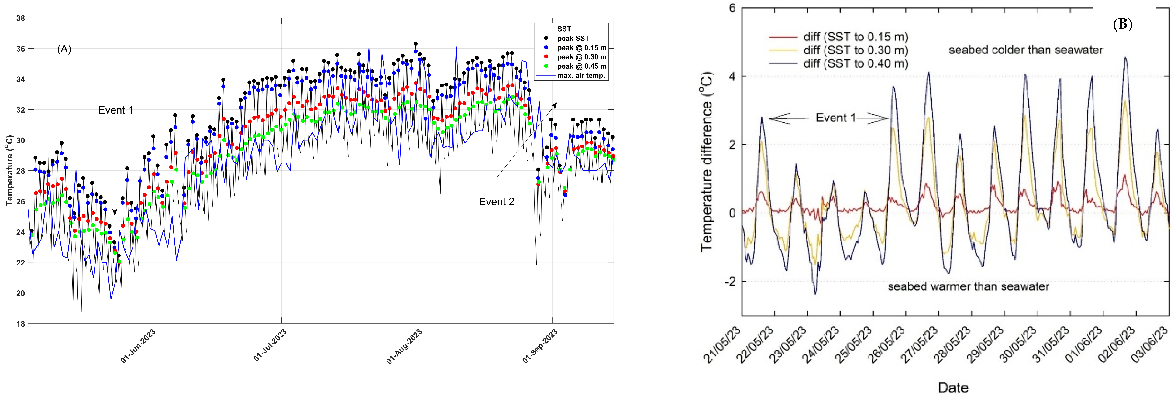
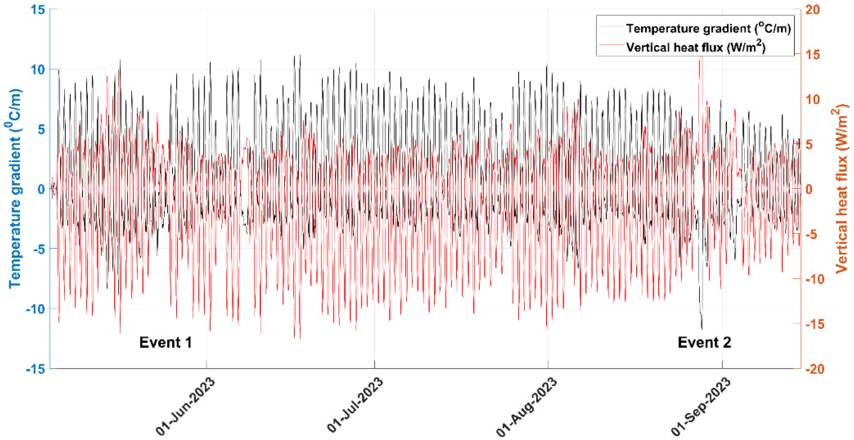
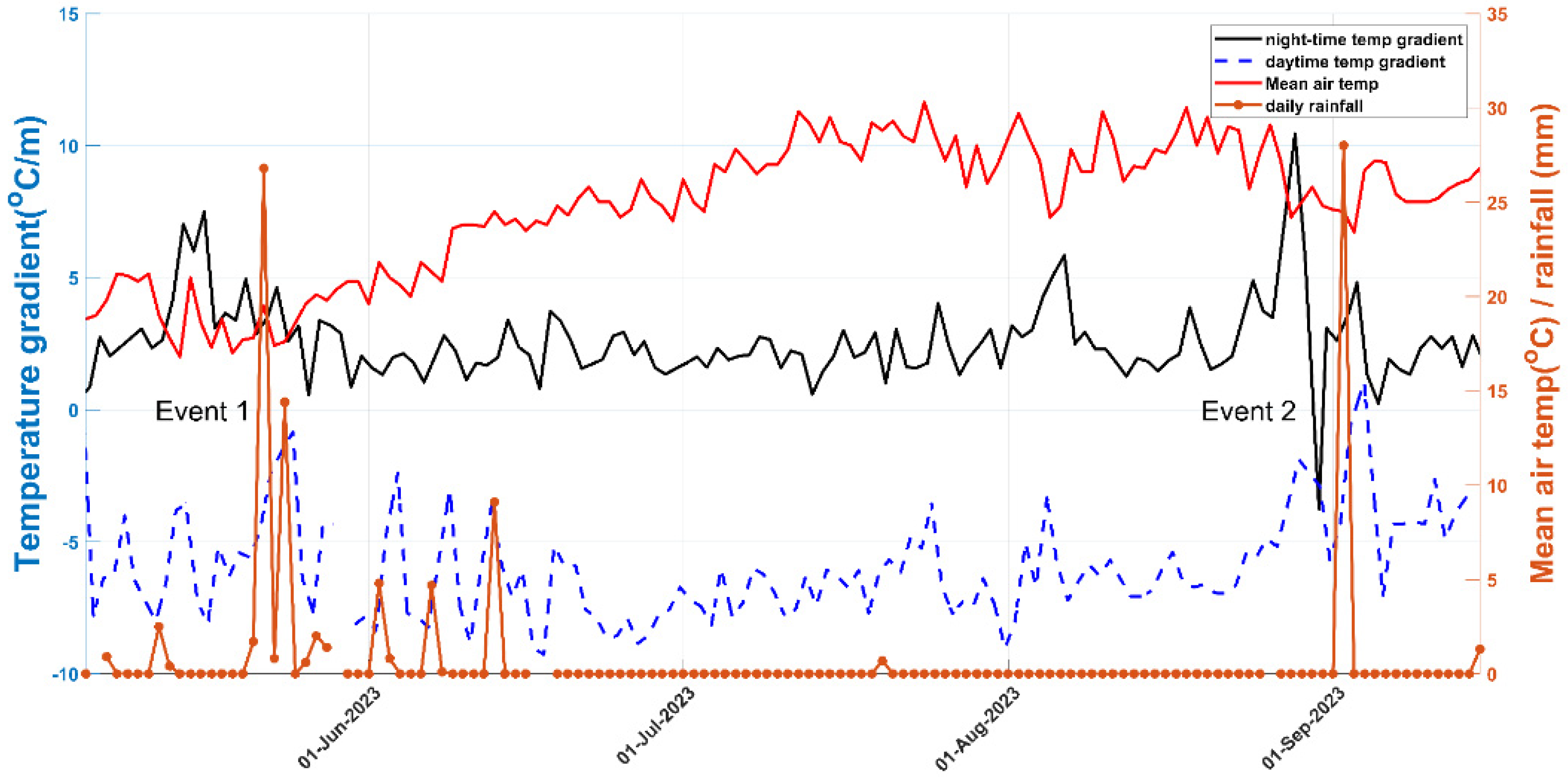
Good quality SST and seabed temperature data were recorded hourly from 10:42, 5 May 2023, to 16:42, 14 September 2023, in a shallow (0.3 m minimum depth) sandy region of the Mar Menor (See Figure 1). The time series was dominated by diurnal fluctuations of up to 5 °C, with a steady increase in temperature punctuated by two storm events (22–24 May and 26 August–5 September), referred to herein as “Event 1” and “Event 2” (see Appendix A Figure A1 and Figure A2 for details). Figure 6A shows the SST during this period and the peak (daytime) temperatures from the four temperature sensors. The maximum air temperature from San Javier airport is also shown. It generally falls below the Mar Menor SST and the seabed temperatures within the shallow water setting of the temperature probe, with notable exceptions taking place in the two events. The peaks at each depth were not synchronous but were delayed by an average of 4.2 ± 2.3 h at the deepest sensor. The diurnal variation in the vertical heat flux was large (−20 to 28 W/m², negative flux is warming downwards). This variation in vertical temperature difference is illustrated for Event 1 in Figure 6B.

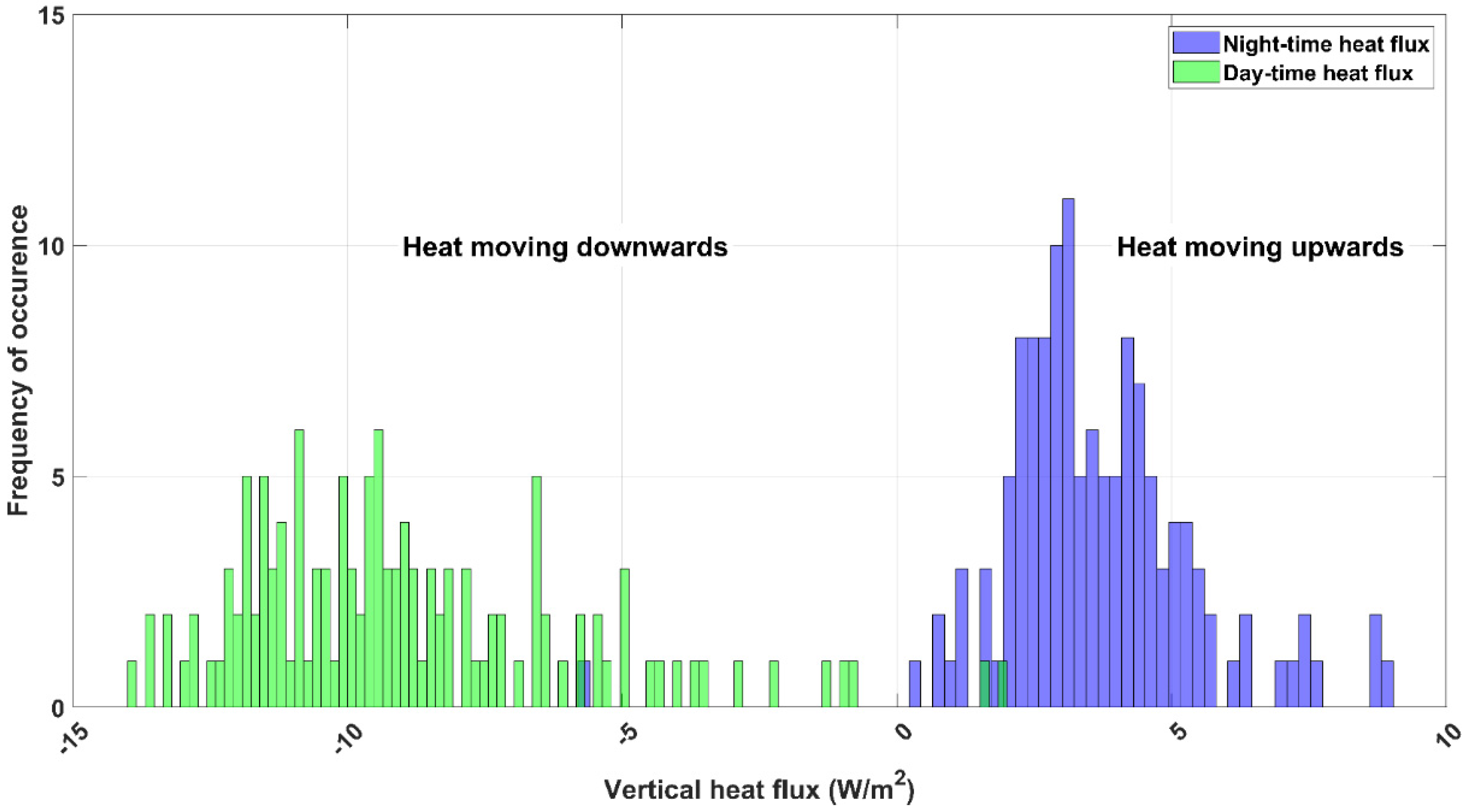
Figure 6B shows that the temperature gradient inverts on a diurnal frequency, illustrating the rapid response of the seabed to changes in heating. That is, the seabed provides heat to the seawater at night. The least-square best fit of the hourly temperature gradients for the measured duration showed a mean daytime value of −5.99 ± 2.05 °C/m (heating of the seabed) and 2.54 ± 1.51 °C/m at night (cooling of the seabed). The estimated vertical heat flux was −8.99 ± 3.08 W/m² during the day and 3.89 ± 2.27 W/m² at night. The “dampening” depth (D) of the temperature gradients is estimated from [38] $D={\left({\displaystyle \frac{2k\ast 86400}{2pi}}\right)}^{0.5}$ to be 2 m into the seabed. Below this depth, the temperature is assumed to be constant [39]. The vertical heat flux for the time series shows strong diurnal oscillations and rapid changes between the peaks in maximum and minimum values (see Appendix A). Figure 7 shows the results for a sub-set of observations for clarity. It appears that the estimates of thermal diffusivity are unstable during periods when the heat flux is changing most (during the day). The nighttime peak temperature gradient (2.54 ± 1.51 °C/m), thermal conductivity (2.01 ± 0.90 W/m.K), and heat flux appear to be constant except for the two rainfall events defined earlier. The daytime temperature gradient appears to be highly sensitive to rainfall and less sensitive to air temperature. This is evident in the two events recorded herein that resulted in 26.8 and 28 mm of rainfall, respectively. Under these events, the temperature gradient reduced to zero with a lag of 24 h.

Similar (but smaller) responses were measured on the 2nd, 6th and 12th of June, 2023, for lower levels of rainfall but similar air temperatures. A similar finding was made by [14]. The time series of the daytime and nighttime peak vertical temperature gradients have been plotted against the mean air temperature (San Javier airport) and daily rainfall (Appendix A Figure A2). The response and lag of the daytime temperature gradient are clear. This contrasts with the nighttime gradients that appear to be influenced by events up to 4 days prior to the rainfall events. Under other times, nighttime temperature gradients were remarkably constant.

The thermal conductivity of the shelly fine sand of this study site should, in theory, remain constant, as should estimates of thermal diffusivity. A test of this was made through the examination of the nighttime heat fluxes, during which time the solar heating of the water column was assumed to be zero (Figure 7). A back calculation (inverting EQ 2) of the mean nighttime estimate of conductivity was 2.01 ± 1.51 W/m.K. This is within the range of values for saturated marine sediments reported by [40]. The estimate of thermal diffusivity using EQ 2 yielded a value of 6.28 × 10⁻⁶ m²/s. The mean value of similar sediments is 1 × 10⁻⁶ m²/s [39,40]. A higher value herein could result from a lower porosity or lower thermal capacity of Mar Menor sediment or from a stronger effect of ground water inflow.

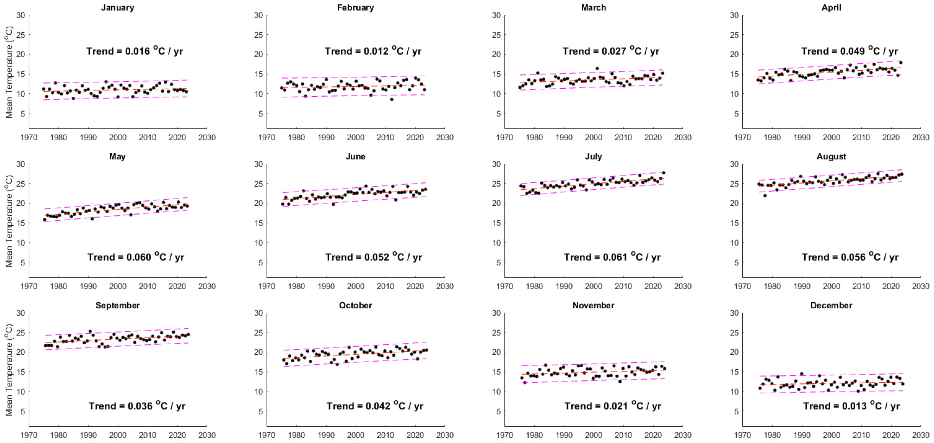
The mean monthly air temperature data from San Javier airport for the period 1980–2024 (inclusive) have been de-seasoned in a similar fashion to the SST for the Western Mediterranean. The trends for each month of the year are presented in Figure 8 and tabulated in Table 1. All but the winter months show significant (p < 0.05) warming trends that peak during the summer months (May–August).

3.3. Step-Wise Regression Analysis

The SST and air temperature data were first used to examine the trends in SST for each month of the year (Figure 5 and Figure 8, respectively). These trends (°C/year) are tabulated in Table 1 (°C/decade) together with the level of confidence (p-value). The summer warming evident in Figure 3 is seen clearly, with the strongest trends between May and October in the HadSST1.1 data. The MODIS (Mar Menor) trends are greater than the Western Mediterranean. However, the level of significance of the trends is generally low. These trends correspond well with the air temperature trends for the region, which do have high levels of significance.

The anomalies in Mar Menor air temperature (MM-air-a), SST (MM-SST-a), SST in the Western Mediterranean (HAD-SST-a) and OISST have been used to explain the changes in SST in the Mar Menor. Anomalies were chosen to remove any local effects. The post-1980 time series (see Figure 4) show that the peaks and troughs appear to coincide reasonably well (see later). As the Mar Menor SST data set from MODIS started in July, 2002, the SST prior to that time was back-filled through a regression of the OISST data with the MODIS data post 2002 (r² = 0.88, n = 538; p < 0.001).

The results of the Spearman rank correlation analysis of NAO, ENSO3,4, IOD, AMO, PDO, CO2-a, sunspots, GDP, MM-air-a and the SST anomaly in the Western Mediterranean (HAD-SST-a) against MM-SST-a are presented in

Table 2. (A) Spearman rank correlation coefficient matrixes of factors from the Mar Menor for the period January, 1980–December, 2024. The level of significance (p-value) is also given. Note the high correlations of MM-SST-a with HAD-SST-a, CO₂-a and GDP (i.e., trends are similar). Also note the high correlations of MM-air-a with HAD-SST-a, MM-SST-a, CO₂-a, GDP, AMO, and IOD. (B) A principal component analysis (10 eigenvectors) showing the correlation matrix as given in (A). PC1 explains 41.9% of the total variance and shows the clustering of CO₂-a, AMO, IOD, and GDP on MM-SST-a and MM-air-a. The intensity of color is added for clarity and is proportional to the trends.

A	MM-Air-a	MM-SST-a	HAD-SST-a	AMO	PDO	ENSO3,4	IOD	NAO	CO2-a	Sunspots	GDP
MM-air-a	1
MM-SST-a	0.73	1				***	p < 0.001
	***					**	p < 0.01
HAD-SST-a	0.78	0.82	1			*	p < 0.1
	***	***				--	not significant
AMO	0.51	0.44	0.55	1
	***	***	***
PDO	−0.25	−0.3	−0.33	−0.3	1
	***	***	***	***
ENSO3,4	−0.03	−0.05	−0.13	0.14	0.24	1
	--	--	**	**	***
IOD	0.39	0.24	0.35	0.22	−0.15	−0.03	1
	***	***	***	***	***
NAO	−0.03	0.03	0	−0.16	0.05	0.02	0.02	1
	--	--	--	***	--	--	--
CO2-a	0.63	0.6	0.72	0.65	−0.47	0.36	0.36	−0.06	1
	***	***	***	***	***	*	***	--
Sunspots	−0.16	−0.11	−0.22	−0.21	−0.05	−0.22	−0.22	0.11	−0.4	1
	***	**	***	***	--	--	***	*	***
GDP	0.58	0.54	0.67	0.65	−0.46	0.39	0.39	−0.08	0.97	−0.48	1
	***	***	***	***	***	*	***	*	***	***
B	PC 1	PC 2	PC 3	PC 4	PC 5	PC 6	PC 7	PC 8	PC 9	PC 10
MM-SST-a	0.345	0.0552	0.357	0.175	0.232	0.181	−0.381	0.0106	0.616	0.325
HAD-SST-a	0.399	0.0566	0.218	−0.00956	0.178	0.151	−0.0747	−0.0203	−0.0641	−0.851
MM-air-a	0.373	0.0127	0.298	0.0461	0.303	0.0339	−0.00799	−0.128	−0.719	0.378
AMO	0.337	−0.142	−0.221	0.344	0.0341	−0.0973	0.566	−0.561	0.222	0.0233
PDO	−0.172	−0.518	0.401	−0.29	0.226	0.271	0.515	0.224	0.124	0.0279
ENSO	0.0112	−0.631	0.182	0.509	−0.243	−0.382	−0.23	0.18	−0.0968	−0.0903
IOD	0.226	0.0597	0.161	−0.496	0.081	−0.799	0.0668	0.0245	0.152	0.014
NAO	−0.0135	0.293	0.591	0.0142	−0.702	0.0659	0.189	−0.175	−0.0107	0.0176
CO2-a	0.417	−0.0135	−0.175	−0.0354	−0.242	0.113	0.128	0.479	0.0272	0.0705
Sunspots	−0.207	0.466	0.164	0.506	0.314	−0.228	0.352	0.423	0.0186	−0.0467
GDP	0.413	0.0292	−0.246	−0.0322	−0.233	0.086	0.173	0.383	−0.0329	0.104

A.

3.4. The Principal Component Analysis and Cross-Correlations

The PCA is conducted on the mean monthly data from 1980 to 2024 (inclusive). The correlation matrix of the PCA is similar to that of the Spearman rank analysis presented in Table 2A. PC1 explains the greatest variance in the data sets (41.7%). It is dominated by CO₂-a and GDP (in magnitude and direction), followed by a clustering of MM-SST-a, MM-air-a, HAD-SST-a and AMO. PC2 (explaining a further 11.5% of the variance) shows an inverse relationship of ENSO3,4 and PDO and a positive contribution of sunspots. These clusterings are echoed to a lesser extent in the remaining principal components.

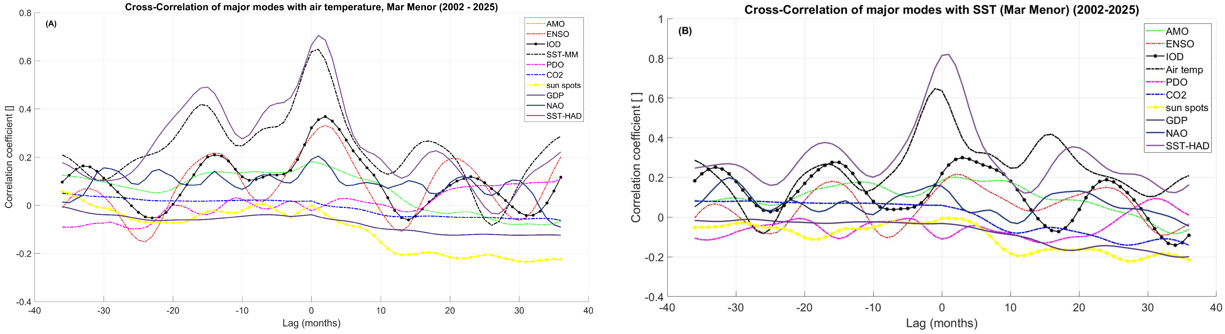
The cross-correlations of parameters relative to MM-air-a and MM-SST-a are shown in Figure 9. The magnitude of the correlations shows significant changes with phase (±36 months) relative to MM-air-a (Figure 9A) and MM-SST-a (Figure 9B). MM-air-a lags MM-SST and HAD-SST by 1 month and lags IOD by 2 months. Also, MM-SST-a lags HAD-SST-a by 1 month. In most cases, correlations vary significantly with changes in lag, and a 16–18-month cyclicity is apparent in some correlations. This cyclicity is also evident in correlations with MM-SST-a.

3.5. The Heat Box Model

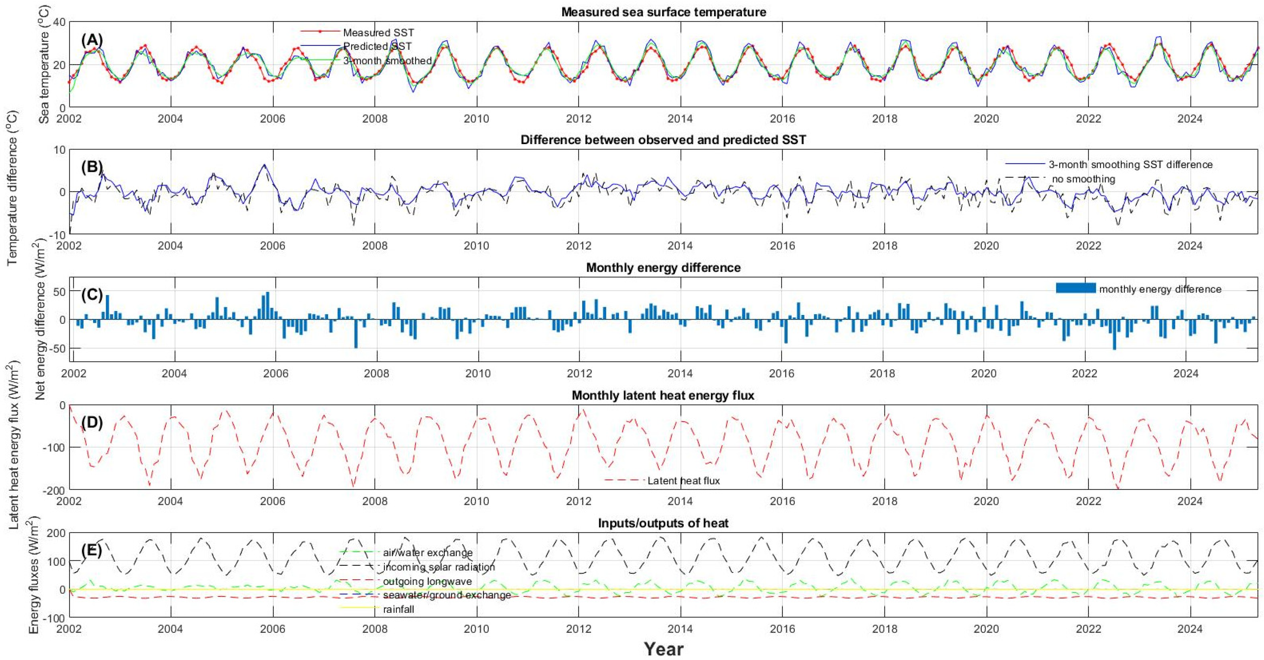
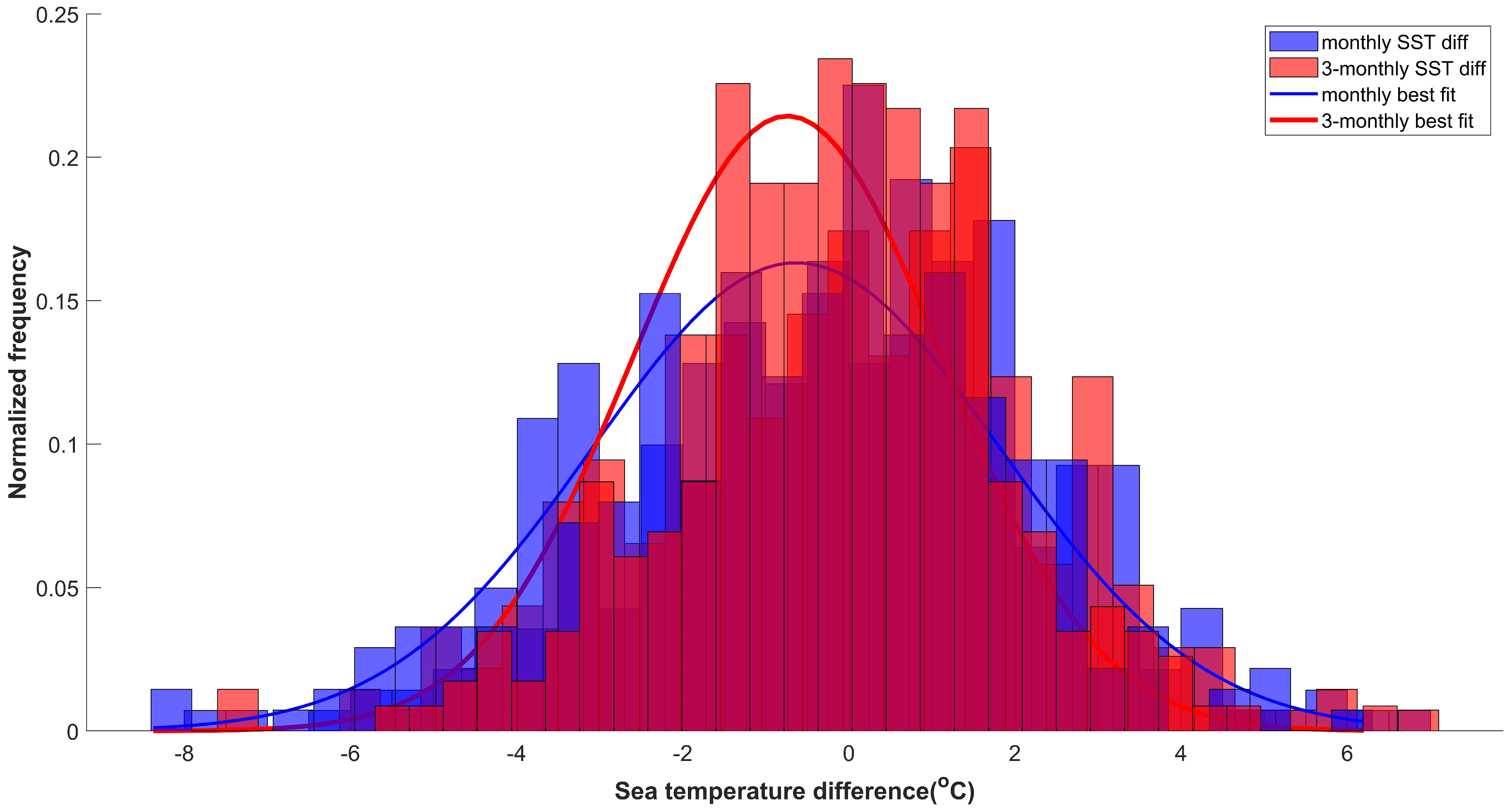
An estimation of the heat budget of the Mar Menor has been evaluated monthly from January 2002 to May 2025. A balance in the heat budget was sought for the sources of heat (principally incoming solar radiation), outgoing heat (long-wave radiation) and the internal exchanges of sensible (air/seawater, rain, river, ground water, and tidal exchanges) and latent heat losses through evaporation. The resulting predicted SST was compared against the measured SST derived from MODIS. A first approximation was made to balance the published annual evaporation (1.35 m/annum, [2]) using EQ 14. This resulted in excessive heat losses that could not be compensated for by other modeled sources. A final reduction in wind speed to 0.7U₁₀ was used, which resulted in an estimated evaporation rate of 0.91 m/annum. Solar radiation at the ground level was balanced best by using a reduction factor of 57% of that at the top of the atmosphere. The best closure with observations was found by neglecting the MERRA 2 average monthly cloud cover, as the scatter was reduced by doing so. The same was true for estimates of the outgoing radiation. The resulting estimated time series of SST is shown in Figure 10A, together with the difference between the observed and predicted SST (Figure 10B). A histogram plot of the differences for the entire time series is shown in Figure 11. The scatter in the differences is Gaussian and yields a standard deviation of ±2.45 °C. Figure 10D,E show the time series of the major sources and sinks of heat: incoming solar radiation, outgoing long-wave radiation, latent heat flux and the different exchanges of sensible heat. The monthly means and annual values of each are given in

Table 3. The estimated sources and sinks of heat (W/m²) to the seawater in the Mar Menor evaluated in the heat box model of this study, together with the results from Rodríguez-Rodríguez and Moreno-Ostos (2006) (RR06) [14] and Martinez-Alvarez et al. (2011) (MA11) [15]. The results show the mean monthly values (and S.D. or standard deviation) for the 281 months of the time series starting January 2002. The long-term average for each month is shown together with the long-term annual average for each source or sink. The Bowen ratio (BR) is also shown. The overall annual average heat loss of 0.67 W/m² in this estimate is within the error margin and so it may be assumed to define a thermal balance. The mean warming of 0.43 °C/decade of the Mar Menor (Table 1) equates to a long-term average heat input of 0.024 W/m² (using $Q= \rho C_{p}h∆t$), which is far too small to be detected within the simple model presented. The influence of tidal exchanges at the three inlets, the sensible exchange through the seabed and the other sources (rain and rivers) were small and had minimal impact on the estimate of SST.

	Q-Latent (W/m2)				Q-Air (W/m2)				Q-Solar (W/m2)			Q-Out (W/m2)			Q-Seabed (W/m2)		Q-Tidal (W/m2)			Q-Rain (W/m2)		Ave	BR
	Mean	S.D	RR06	MA11	Mean	S.D	RR06	MA11	Mean	S.D	RR06	Mean	S.D	RR06	Mean	S.D	Mean	S.D	MA11	Mean	S.D	(W/m2)	[]
Jan	−42.6	14.5	−56.4	−36.7	−5.9	7.5	−4.3	−5.8	87.9	6.2	107.7	−39.4	9.31	−29.4	0.04	0.01	−0.01	0.07	2.09	0.02	0.05	0.01	−0.12
Feb	−46.6	15.8		−40.7	5.1	10.5		−9.1	73.7	4.6		−42.9	0.77		0.02	0.01	−0.06	0.03	1.33	−0.01	0.03	−1.54	0.16
Mar	−63.7	12.6		−61.6	18.7	12.6		−11.9	83.2	5.1		−44.6	1.03		−0.01	0.02	−0.09	0.03	−0.56	−0.14	0.12	−0.95	0.30
April	−86.6	10.9	−113.7	−104.3	28.8	14.9	−26	−28.4	114.7	7.2	233.1	−47	1.19	−41	−0.05	0.02	−0.26	0.07	−2.71	−0.19	0.18	1.34	0.33
May	−120.8	16.1		−133.2	35.1	13.1		−34.4	152.2	7.9		−49	0.89		−0.08	0.01	−1.14	0.22	−4.15	−0.13	0.12	2.31	0.29
June	−171.4	16.4		−157	32.6	11.2		−28.9	192	9.7		−50	0.43		−0.1	0.01	−1.01	0.18	−4.4	−0.08	0.08	0.29	0.19
July	−213.5	23.4	−133.3	−175.6	21.2	4.1	−27	−30.2	224.7	12.6	213.5	−49.1	0.76	−51.5	−0.08	0.01	0.07	0.42	−3.2	−0.02	0.02	−2.39	0.10
Aug	−234.1	24.3		−175.8	3.6	9.9		−25.5	246.4	7.4		−47	1.04		−0.05	0.02	1.25	0.49	−1.76	−0.01	0.02	−4.27	0.02
Sept	−204	18.5		−134	−8.6	13		−22.3	241.3	4.7		−44.3	1.38		−0.01	0.02	0.14	0.05	−0.45	0.1	0.13	−2.20	−0.04
Oct	−156.8	21.1	−82.2	−92.6	−19.8	18.3	−21	−19.3	209.8	9	90.3	−42	1.14	−59.6	0.03	0.02	0.73	0.19	1.32	0.18	0.16	−1.12	−0.13
Nov	−104.9	15.8		−60.6	−22.1	17		−15.2	165.8	8.8		−40.9	0.36		0.05	0.01	−0.03	0	2.39	0.17	0.14	−0.27	−0.21
Dec	−62.6	10.8		−43.8	−16.5	6.3		−5.3	125.3	8.3		−40.9	0.45		0.05	0.01	−0.44	0.13		0.1	0.14	0.72	−0.26
Ave=	−125	16.68	−96.40	−101.33	6.02	11.53	−19.58	−19.69	159.75	7.63	161.15	−44.76	1.56	−45.38	−0.02	0.01	−0.07	0.16	−0.92	0.00	0.10	−0.67	0.05

.

The influence of tidal exchanges at the three inlets, the sensible exchange through the seabed and the other sources (rain and rivers) were small and had minimal impact on the estimate of SST in the Mar Menor.

4. Discussion

SST trends in the north Atlantic during the 20th century were examined by [41], with the conclusion that “no one should doubt that human activity is largely responsible”, and that the increasing droughts in the Mediterranean region are likely driven in part by the AMO [42]. The data examined herein (Figure 2) suggest that, for the Western Mediterranean at least, the long-term trends are also driven by the AMO (which has been increasing in magnitude since circa 1970). The 1977/80 change in the SST regime found herein for the W. Mediterranean is close to the 1976 regime change evident in the Pacific Ocean [37], which corresponds to a shift in ENSO and PDO patterns and the beginning of the current global warming trend. It is tempting to link the warming of the Mar Menor since circa 1980 to this regime change, and to increases in CO₂, as there is a strong correlation between the two (i.e., they are both generally rising). However, the lack of a long-term trend in SST pre-1980 (when CO₂ was rising) and the lack of correlation in the cross-correlation analyses suggest that regional/local factors may be more significant drivers of temperature change. The systematic increase in magnitude of the AMO since circa 1970, together with the peaking of the Eddy cycle of solar activity as proposed by [37], may be the main driver of the trends found herein. The AMO presently appears to be at its peak and is due to decrease during the next 30 years [37]. If this is so, then we could also anticipate a reduction in SST in the Mar Menor over this time period.

The PCA analysis conducted on mean monthly data from 1980 to 2024 showed that the strongest correlation of SST in the Mar Menor was with SST in the adjacent coastal waters. As shown in the box model, this is not due to mixing across the inlets. Air temperature showed the next strongest correlation with SST in the Mar Menor, with zero lag. The fact that only the IOD showed significant cross-correlations perhaps suggests that local drivers are largely more important to the details of local temperature.

The fluxes of energy into (during the day) and out of (during the night) the Mar Menor seabed are significant at diurnal time scales. The delay in peak temperature with depth has not been considered as a factor in the estimation of these heat fluxes. The sensors were initiated sequentially, with an approximate 5 min delay in each case. The sample rate of 1 h is considered too coarse to evaluate the travel time of heat with depth.

The heat box model for the seawater of the Mar Menor has been used to balance the sources and sinks of heat. An estimated evaporation rate of 0.91 m is less than that presented by [2]. A higher evaporation rate (governed by the selection of the appropriate height of wind speed) resulted in excessive cooling in summer. Non-seasonal scatter in the estimated SST error remains to be explained. The years 2012–2014 exhibited relatively low summertime evaporation rates, a period of time when the predicted SST showed the lowest scatter. This may suggest that the greatest source of error is in the estimation of the latent heat loss through evaporation.

A multi-year trend in the energy balance appears to be present in the time series (Figure 10C). This seems to be related to changes in the summertime peak in the latent heat loss (Figure 10D). Notice that, in the years 2012 to 2014, the summertime heat losses are relatively low. This is the period that shows the lowest scatter in predictions. During the periods 2006 to 2010 and post 2016, summertime heat losses are relatively high. The peaks in the air/seawater exchange of sensible heat (Figure 10E) also appear to vary inversely with the peaks in latent heat loss: they are relatively low, with low seasonal variation from 2002 to 2007. The histogram of the predicted differences between the model output and measured SST in Figure 11 shows that a 3-month smoothing of predictions reduced the scatter. This suggests that there is a possible month-long inertia in response to heating not represented in the monthly mean data. The addition of tidal mixing results in a slight cool bias in the results. However, it could be omitted from the heat budget estimate (as done by MA11) without a loss of information. The overall annual loss of −0.67 W/m² in the heat budget estimate is within the estimated error margin, and so it may be assumed that the model defines a thermal balance. A mean of 0.43 °C/decade warming of the Mar Menor seawater (see Table 1) for a mean water depth of 4.5 m equates to a long-term average heat input of 0.024 W/m², which is far too small to be detected within the simple model presented herein.

Rainfall has a significant impact on the seabed temperature profile. During Event 1 (23–26 May 2023), the daytime temperature gradient was almost eliminated, whereas the seabed relative warming at night was enhanced to a maximum of 2.4 °C. The same occurred during Event 2 (26–28 August 2023), but to a greater degree. During this event, the seabed remained consistently warmer than the seawater by a maximum of 5.0 °C. The heat was subsequently returned to the water column in the ensuing 24 h. The air temperature and wind speed were not unusual during these events.

The effects of freshwater inflow and rainfall were neglected in the estimates of the heat budget of [15]. The data presented herein (Table 3) suggest that doing so would have no material impact on their results. The impact of heat exchange with the ground, however, can have a considerable impact on the day–night vertical temperature gradients at diurnal time scales if not longer, cooling seawater by day and warming it by night.

MA11 estimated the mean annual Bowen ratio to be 0.19, which is typical of Mediterranean coastal lagoons: the data herein suggest that it varies throughout the year from −0.26 in December to 0.33 in April (mean = 0.05 ± 0.21). MA11 shows a slightly lower latent heat loss than was found herein (see Table 3), which can be explained through differences in the air vapor pressure and relative humidity. Figure 4 and Figure 10 illustrate that the period 2003 to 2006 exhibited relatively mild winters and a narrower range of seasonal SST. This may be due in part to the greater than average summertime latent heat losses during this period. Much of the differences between MA11 and those presented herein are considered to be due to the decadal changes in heat sources and sinks, many of which are considered to be due to changes in the impact of the AMO and possibly the IOD.

Ref. [14] estimated that the heat loss as long-wave radiation from a small lagoon in Spain was 70% of the non-advective heat losses, and evaporation accounted for 20% of the total energy heat losses. The values estimated herein were 26% and 73%, respectively (see Table 3), i.e., the inverse. The systematic increase in annual heat flux due to evaporation since 2006 (evident in Table 3) may be due to the long-term warming trends in air temperature and SST.

5. Conclusions

Long-term records of SST from the Western Mediterranean indicate that there was no trend prior to circa 1980, but that the SST appeared to respond on a decadal scale to the AMO and on an annual scale to the NAO. Post 1980, the SST showed significant increases of 0.34 °C/decade (summer maximum) and 0.21 °C/decade (winter minimum). This is compared with 0.39 °C/decade for the Mediterranean Sea as a whole. There were significant (p < 0.05) increases for all months of the year. The onset of warming appears to lag the 1976 “regime shift” in SST in the Pacific Ocean that is attributed to changes in ENSO and PDO.

Air temperature trends in the Mar Menor region have shown significant systematic warming since circa 1980 at all months of the year. Peak warming takes place in the summer months (maximum of 0.61 °C/decade in July). A Spearman rank correlation of the SST anomaly in the Mar Menor (1980–2024) showed strong and significant correlations with (in order) SST in the Western Mediterranean, CO₂, Spanish national GDP, AMO and IOD (i.e., the trends are similar). It was inversely correlated with the PDO and sunspot activity. A similar clustering of drivers resulted from a PCA analysis of variables. Cross-correlation, by contrast (which emphasizes the raw data), showed no significant influence for the global drivers (with the possible exception of IOD).

Measured heat exchanges between the seabed and the water column in the Mar Menor showed strong diurnal inversions of the temperature gradient, resulting in a daytime heat flux of −8.99 ± 3.08 W/m² and a nighttime reversal of 3.89 ± 2.27 W/m² and resulting in a warming of the seabed with time. The estimated depth of temperature fluctuations in the seabed was 2 m. The 5 months of hourly measurements showed that rainfall had the greatest effect on the seabed temperature and heat exchange with the water column. It was also clear that a sampling rate of 1/hour is insufficient to accurately predict the thermal diffusivity or thermal conductivity of the seabed sediments. A reasonable estimate of heat flux, however, was achieved using the diurnal maxima and minima at a sample rate of 1/hour. The probe data suggested that the long-term (monthly) exchange of heat between the water column and the seabed was small and mimicked the seasonal heating of the Mar Menor.

A heat budget box model of SST in the Mar Menor was developed as an extension of that presented by MA11. The predictions used added inputs that included tidal mixing, rainfall, groundwater inflow, and river inflow. A balance of 0.6 ± 2.45 °C was derived over a prediction period from January, 2002, to December, 2024, resulting in an estimated heat loss of −0.67 W/m². A thermal balance was only possible by using 70% of the wind speed in estimations of the evaporation rate and heat losses. This resulted in an evaporation rate of 0.91 m/annum, which is less than the 1.31 m/annum previously quoted. The results herein agree with MA11 that the dominant sources and sinks of heat are solar radiation and evaporation; other terms appear insignificant to the outcome. The incoming solar and outgoing latent heat losses (through evaporation) were generally higher (−125 ± 16.7 W/m²) than those estimated by RR06 (−96.4 W/m²) in an adjacent lagoon and based upon daily measurements made over a single year and closer to those reported by MA11 (−101.3 W/m²). If these results are correct, then the latent heat loss from the Mar Menor appears to have increased since 2006.

References

1. Álvarez-Rogel, J.; Barberá, G.G.; Maxwell, B.; Guerrero-Brotons, M.; Díaz-García, C.; Martínez-Sánchez, J.J.; Sallent, A.; Martínez-Ródenas, J.; González-Alcaraz, M.N.; Jiménez-Cárceles, F.J.; et al. The case of Mar Menor eutrophication: State of the art and description of tested nature-based solutions. Ecol. Eng. 2020, 158, 106086. [Google Scholar] [CrossRef] [Scilit]
2. Senent-Aparacio, J.; Lopez-Ballesteros, A.; Nielsen, A.; Trolle, D. A holistic approach for determining the hydrology of the mar menor coastal lagoon by combining hydrological & hydrodynamic models. J. Hydrol. 2021, 603, 127150. [Google Scholar] [CrossRef] [Scilit]
3. Conesa, H.M.; Jiménez-Cárceles, F. The Mar Menor lagoon (SE Spain): A singular natural ecosystem threatened by human activities. Mar. Pollut. Bull. 2007, 54, 839–849. [Google Scholar] [CrossRef] [Scilit] [PubMed]
4. Álvarez-Rogel, J.; Ramos-Aparicio, M.J.; Delgado-Iniesta, M.J.; Arnaldos-Lozano, R. Metals in soils and above-ground biomass of plants from a salt marsh polluted by mine wastes in the coast of the Mar Menor Lagoon, SE Spain. Fresenius Environ. Bull. 2004, 13, 274–278. [Google Scholar]
5. Jiménez-Martínez, J.; García-Aróstegui, J.L.; Hunink, J.; Contreras, S.; Baudron, P.; Candela, L. The role of groundwater in highly human-modified hydrosystems: A review of impacts and mitigation options in the Campo de Cartagena-Mar Menor coastal plain (SE Spain). Environ. Rev. 2016, 24, 377–392. [Google Scholar] [CrossRef] [Scilit]
6. Byrne, R.H.; Kump, L.R.; Cantrell, K.J. The influence of temperature and pH on trace metal speciation in seawater. Mar. Chem. 1988, 25, 163–181. [Google Scholar] [CrossRef] [Scilit]
7. Fong, P.; Zedler, J.B. Temperature and light effects on the seasonal succession of algal communities in shallow coastal lagoons. J. Exp. Mar. Biol. Ecol. 1993, 171, 259–272. [Google Scholar] [CrossRef] [Scilit]
8. Pérez-Matín, M.A. Understanding Nutrient Loads from Catchment and Eutrophication in a Salt Lagoon: The Mar Menor Case. Water 2023, 15, 3569. [Google Scholar] [CrossRef] [Scilit]
9. Pérez-Ruzafa, A.; Fernández, A.I.; Marcos, C.; Gilabert, J.; Quispe, J.I.; García-Charton, J.A. Spatial and temporal variations of hydrological conditions, nutrients and chlorophyll a in a Mediterranean coastal lagoon (Mar Menor, Spain). Hydrobiologia 2005, 550, 11–27. [Google Scholar] [CrossRef] [Scilit]
10. Rodriguez-Puig, J.; Rodellas, V.; Diego-Feliu, M.; Alcolea, A.; Jiménez-Martínez, J.; Alorda-Montiel, I. Seasonality of submarine groundwater discharge pathways in a coastal lagoon revealed by radium isotopes: The importance of porewater exchange in summer. J. Hydrol. 2025, 661, 133616. [Google Scholar] [CrossRef] [Scilit]
11. Bauraï, L.; Logez, M.; Laplace-Treyture, C.; Argillier, C. How do eutrophication and temperature interact to shape the commnity structures of phytoplankton and fish in lakes? Water 2020, 122, 779. [Google Scholar] [CrossRef] [Scilit]
12. Lloret, J. LAGOONS Deliverable D2.1c: The Mar Menor Lagoon—Current Knowledge Base and Knowledge Gaps. Technical Report; 65p. 2012. Available online: https://www.researchgate.net/publication/348453752_LAGOONS_Deliverable_D21c_The_Mar_Menor_Lagoon_-_Current_knowledge_base_and_knowledge_gaps (accessed on 12 March 2024).
13. García-Oliva, M.; Pérez-Ruzafa, Á.; Umgiesser, G.; McKiver, W.; Ghezzo, M.; De Pascalis, F.; Marcos, C. Assessing the Hydrodynamic Response of the Mar Menor Lagoon to Dredging Inlets Interventions through Numerical Modelling. Water 2018, 10, 959. [Google Scholar] [CrossRef] [Scilit]
14. Rodríguez-Rodríguez, M.; Moreno-Ostos, E. Heat budget, energy storage and hydrologycal regime in a coastal lagoon. Limnologica 2006, 36, 217–227. [Google Scholar] [CrossRef] [Scilit]
15. Martínez-Alvarez, V.; Gallego-Elvira, B.; Maestre-Valero, J.F.; Tanguy, M. Simultaneous solution for water, heat and salt balances in a Mediterranean coastal lagoon (Mar Menor, Spain). Estuar. Coast. Shelf Sci. 2011, 91, 250–261. [Google Scholar] [CrossRef] [Scilit]
16. De Pascalis, F.; Pérez-Ruzafa, A.; Gilabert, J.; Marcos, C.; Umgiesser, G. Climate change response of the Mar Menor coastal lagoon (Spain) using a hydrodynamic finite element model. Estuar. Coast. Shelf Sci. 2012, 114, 118–129. [Google Scholar] [CrossRef] [Scilit]
17. Lau, Y.L. Temperature effect on settling velocity and deposition of cohesive sediments. J. Hydraul. Res. 1994, 32, 41–51. [Google Scholar] [CrossRef] [Scilit]
18. Ramalingam, S.; Chandra, V. Experimental investigation of water temperature influence on suspended sediment concentration. Environ. Process. 2019, 6, 511–523. [Google Scholar] [CrossRef] [Scilit]
19. Bellino, A.; Mangano, M.C.; Baldantoni, D.; Russell, B.D.; Mannino, A.M.; Mazzola, A.; Vizzini, S.; Sarà, G. Seasonal patterns of biodiversity in Mediterranean coastal lagoons. Divers. Distrib. 2019, 25, 1512–1526. [Google Scholar] [CrossRef] [Scilit]
20. Al-Banaa, K.; Rakha, K. Seasonal variability of temperature measurements in shallow bay. J. Coast. Res. 2009, 56, 782–786. [Google Scholar]
21. Amos, C.L.; Umgiesser, G.; Ghezzo, M.; Kassem, H.; Ferrarin, C. Sea surface temperature trends in Venice lagoon and the adjacent waters. J. Coast. Res. 2016, 33, 385–395. [Google Scholar] [CrossRef] [Scilit]
22. Kassem, H.; Amos, C.L.; Thompson, C.E.L. Sea surface temperature trends in the coastal zone of southern England. J. Coast. Res. 2022, 39, 18–31. [Google Scholar] [CrossRef] [Scilit]
23. O’Carroll, A.G.; Armstrong, E.M.; Beggs, H.M.; Bouali, M.; Casey, K.S.; Corlett, G.K. Observational needs of sea surface temperature. Front. Mar. Sci. 2019, 6, 420. [Google Scholar] [CrossRef] [Scilit]
24. Farouki, O.T. Thermal Properties of Soils; Technical Publications: Maharashtra, India, 1986; ISBN 0-87849-055-8. [Google Scholar]
25. Rayner, N.A.; Parker, D.E.; Horton, E.B.; Folland, C.K.; Alexander, L.V.; Rowell, D.P.; Kent, E.C.; Kaplan, A. Global analyses of sea surface temperature, sea ice, and night marine air temperature since the late nineteenth century. J. Geophys. Res. 2003, 108, 4407. [Google Scholar] [CrossRef] [Scilit]
26. Garcia-Monteiro, S.; Sobrino, J.A.; Julien, Y.; Soria, G.; Skokovic, D. Surface temperature trends in the Mediterranean Sea from MODIS data during years 2003–2019. Reg. Stud. Mar. Sci. 2022, 49, 102086. [Google Scholar] [CrossRef] [Scilit]
27. Findley, D.F.; Monsell, B.C.; Bell, W.R.; Otto, M.C.; Chen, B.C. New capabilities and methods of the X-12_ARIMA seasonal-adjustment program. J. Bus. Econ. Stat. 1998, 16, 127–152. [Google Scholar] [CrossRef] [Scilit]
28. Williams, G.P. Chaos Theory Tamed; Taylor and Francis: London, UK, 1997; 499p. [Google Scholar]
29. Becker, G.A.; Pauly, M. Sea surface temperature changes in the North Sea and their causes. J. Mar. Sci. 1996, 53, 887–898. [Google Scholar] [CrossRef] [Scilit]
30. Xue, M.; Li, T. To what extent does ENSO rectify the tropical Pacific mean state? Clim. Dyn. 2023, 61, 3875–3891. [Google Scholar] [CrossRef] [Scilit]
31. Gill, A.E. Atmosphere-Ocean Dynamics; Academic Press: Paris, France, 1982; 663p. [Google Scholar]
32. Csanady, G.T. Air-Sea Interaction; Cambridge University Press: Cambridge, UK, 2012; 239p. [Google Scholar]
33. Sultan, S.A.R.; Ahmad, F. Heat budget of the coastal water of Kuwait: A preliminary study. Estuar. Coast. Shelf Sci. 1994, 38, 319–325. [Google Scholar] [CrossRef] [Scilit]
34. Humlum, O. The State of the Climate 2021; Report 51; The Global Warming Policy, Foundation: London, UK, 2022; 54p. [Google Scholar]
35. Hegerl, G.C.; Brönnimann, S.; Cowan, T.; Friedman, A.R.; Hawkins, E.; Iles, C.; Müller, W.; Schurer, A.; Undorf, S. Causes of climate change over the historical record. Environ. Res. Lett. 2019, 14, 123006. [Google Scholar] [CrossRef] [Scilit]
36. Cusack, S.; Cox, T. Brief communication: Drivers of the recent warming of the Mediterranean Sea, and its implications for hail risk. Nat. Hazards Earth Syst. Sci. 2025, 25, 2963–2972. [Google Scholar] [CrossRef] [Scilit]
37. Vinõs, J. Climate of the Past, Present and Future. A Scientific Debate; Critical Science Press: Madrid, Spain, 2022; 740p. [Google Scholar]
38. Harrison, S.J.; Phizacklea, A.P. Temperature fluctuation in muddy intertidal sediments, Forth estuary, Scotland. Estuar. Coast. Shelf Sci. 1987, 24, 279–288. [Google Scholar] [CrossRef] [Scilit]
39. Bullard, E.C. The flow of heat through the floor of the Atlantic Ocean. Proc. R. Soc. A 1954, 222, 408–429. [Google Scholar] [CrossRef] [Scilit]
40. Foucher, J.P.; Nouzé, H.; Henry, P. Variability of heat flow at the western Mediterranean continental margin. Mar. Geol. 2002, 182, 109–128. [Google Scholar]
41. Cane, M.A.; Lee, D.E. What do we know about the climate of the next decade? In Food Security and Sociopolitical Stability; Barrett, C.B., Ed.; Oxford University Press: Oxford, UK, 2013; pp. 64–94. [Google Scholar]
42. Marullo, S.; Artale, V.; Santoleri, R. The SST multidecadal variability in the Atlantic-Mediterranean region and its relation to AMO. J. Clim. 2011, 24, 4385–4401. [Google Scholar] [CrossRef] [Scilit]
Figure 1. A location diagram of the Mar Menor lagoon, Spain. Also shown are the key locations referred to in the text.
Water 18 00533 g001
Figure 2. (A) A time series of mean monthly SST in the Western Mediterranean between 1900 and 2024 (inclusive). The short-term peaks and troughs appear to map to those of the NAO (B), while the long-term trends in SST appear to be controlled by the AMO (C). More detailed correlations are examined further in the text. Note that the temperature appears to increase after circa 1977; no clear long-term trend in SST is apparent before this date.
Water 18 00533 g002
Figure 3. A sub-set of the data set in Figure 2 showing the maximum and minimum mean monthly SST from 1932 to 1979 (no trends found) and 1980 to 2024 (inclusive). Maximum and minimum SST trends post circa 1980 show significant upward trends. Maxima appear to be increasing faster (0.34 °C/decade) than the minima (0.21 °C/decade). The seasonal range in SST thus appears to be increasing steadily with time.
Water 18 00533 g003
Figure 4. Temperature anomalies for the period 1980–2024 (inclusive) showing the Mar Menor SST anomaly, air temperature anomaly (San Javier airport), HadSST1.1 (Western Mediterranean) anomaly, and OISST anomaly. The trends in SST of the Mar Menor are similar to those further afield and also co-vary with air temperature. However, the Mar Menor SST anomaly appears lower than other anomalies, particularly during winter. The 1991–1993 cooling appears to correspond to the eruption of Mount Pinatubo in June 1991 (see [37] for discussion).
Water 18 00533 g004
Figure 5. SST trends from the Western Mediterranean from 1980 to 2024 (inclusive) for each month of the year. The trends are based on a least-square best fit regression analysis. All trends are significant at p < 0.01. Also shown are the 95% confidence limits of the fits. Notice the greatest warming takes place in the summer and the lowest takes place in the winter. The warming rates are listed in Table 1.
Water 18 00533 g005
Figure 6. (A). SST measured at h = 0.15 m at the probe site (see Figure 1) together with the temperatures within the seabed at depths of 0.15, 0,30 and 0.45 m. Also shown is the daily maximum air temperature at San Javier airport. A general increase in both SST and air temperature is noted despite strong diurnal fluctuations. SST leads, and is greater than, air temperature Also note the two cooling events (24th May and 27th August) due to heavy rainfall. (B). The difference in temperatures between the four depths expanded to show the 24th May rainfall event. Note the near 6 °C swing in temperatures compared to SST at 0.45 m depth, which was muted during the May event.
Water 18 00533 g006
Figure 7. The nighttime peak temperature gradients (mean = 2.54 ± 1.51 °C/m), the estimated vertical heat flux (mean = 3.89 ± 2.27 W/m2) and the back-estimated thermal conductivity (2.01 ± 0.90 W/m.K) derived from the nighttime temperature gradients measured with the thermal probe. Notice the reasonably steady estimates except for the two rainfall events defined in the text (also see Appendix A Figure A2).
Water 18 00533 g007
Figure 8. Mean air temperature trends of each month for the Mar Menor for the period 1980–2024 (inclusive). As with the SST, the greatest warming takes place in the summer months and the lowest during winter. The trends are tabulated in Table 1. Trends from March to October are significant.
Water 18 00533 g008
Figure 9. (A) Cross-correlations of key parameters with air temperature (San Javier airport) for lags of −36 to 36 months. The strongest correlation (at zero lag) is with the SST in the Western Mediterranean. This is followed by SST in the Mar Menor, IOD and ENSO3,4. (B) Cross-correlations of key parameters with SST in the Mar Menor. The strongest correlation is with SST (Western Mediterranean) followed by air temperature and IOD. Note the lack of significant correlation of other parameters at all lags. Note the 14–16-month cyclicity in correlation with IOD and ENSO3,4.
Water 18 00533 g009
Figure 10. (A) A time series of the heat box model of the Mar Menor evaluated monthly between January 2002 and May 2025. (B) The heat budget simulates the observed SST with a non-seasonal Gaussian scatter with a mean of near-zero and an SD of ±2.45 °C (see Figure 11). (CE) show the time series of the estimated major sources and sinks of heat. Note the multi-year periods of negative and positive energy balance that is evident in the changes in latent heat loss shown in (D).
Water 18 00533 g010
Figure 11. Histograms of the difference (diff) between observed and predicted SST from the heat box model of this study together with Gaussian best fits (1-month and 3-month averages). There is little bias in the data (0.06 °C). However, the standard deviation of the scatter is large (±2.45 °C). The 3-month averaging reduces the scatter in predictions and draws the predictions closer to the observed values. The Gaussian shape of the scatter suggests that the errors in the model are random, with no seasonal residual signal.
Water 18 00533 g011