Article

Bridging Time-Scale Mismatch in WWTPs: Long-Term Influent Forecasting via Decomposition and Heterogeneous Temporal Attention

1
Department of Environmental Science and Engineering, Fudan University, Shanghai 200433, China
2
Shanghai Environmental Protection (Group) Co., Ltd. (SEPG), Shanghai 200433, China
*
Author to whom correspondence should be addressed.
Water 2026, 18(3), 295; https://doi.org/10.3390/w18030295
Submission received: 24 December 2025 / Revised: 18 January 2026 / Accepted: 20 January 2026 / Published: 23 January 2026

Abstract

The time-scale mismatch between rapid influent fluctuations and slow biochemical responses hinders the stability of wastewater treatment plants (WWTPs). Existing models often fail to capture shock signals due to noise interference (“signal pollution”). To address this, we propose the HD-MAED-LSTM model, which employs a “decompose-and-conquer” strategy. Targeting the dynamic characteristics of different components, this study innovatively designs heterogeneous attention mechanisms: utilizing Long-term Dependency Attention to capture the global evolution of the trend component, employing Multi-scale Periodic Attention to reinforce the cyclic patterns of the seasonal component, and using Gated Anomaly Attention to keenly capture sudden shocks in the residual component. In a case study, the effectiveness of the proposed model was validated based on one year of operational data from a large-scale industrial WWTP. HD-MAED-LSTM outperformed baseline models such as Transformer and LSTM in the medium-to-long-term (10-h) prediction of COD, TN, and TP, clearly demonstrating the positive role of differentiated modeling. Notably, in the core task of shock load early warning, the model achieved an F1-Score of 0.83 (superior to Transformer’s 0.77 and LSTM’s 0.67), and a Mean Directional Accuracy (MDA) as high as 0.93. Ablation studies confirm that the specialized attention mechanism is the key performance driver, reducing the Mean Absolute Error (MAE) by 56.7%. This framework provides precise support for shifting WWTPs from passive response to proactive control.

1. Introduction

Municipal Wastewater Treatment Plants (WWTPs) serve as critical infrastructure for safeguarding urban water environment security. However, their stable and efficient operation is continuously adversely affected by drastic fluctuations in the influent. In particular, the rapid water quality fluctuations caused by upstream discharges form a fundamental time-scale mismatch with the slow response dynamics of core biochemical processes such as the activated sludge process (typically featuring a Hydraulic Retention Time (HRT) of 6 to 12 h) [1]. This can lead to low efficiency in the wastewater treatment system or even system collapse [2]. Existing WWTPs primarily rely on lagged feedback control strategies (such as PID control based on DO probes). This passive response forces plants to adopt a high-redundancy “worst-case” operational mode, resulting in tremendous energy waste [3]. Jamaludin et al. (2024) noted that the aeration process is the most energy-intensive component in WWTPs, accounting for approximately 65–70% of the total energy consumption [4]. Research by Faisal et al. (2023) further emphasized that pumping and aeration systems collectively account for over 80% of the total WWTP energy consumption; therefore, optimal control targeting these units is a critical path for achieving energy saving and consumption reduction [3].
To achieve forward-looking “proactive pre-control,” the research focus has shifted from traditional mechanistic models to data-driven time series prediction algorithms. Early Machine Learning (ML) models demonstrated potential in predicting specific indicators. For instance, Arismendy et al. (2020) developed an intelligent system based on Multi-Layer Perceptron (MLP) to predict the Chemical Oxygen Demand (COD) at the bioreactor inlet, achieving a Mean Absolute Percentage Error (MAPE) of 10.8% over a one-day prediction window, proving the effectiveness of neural networks in handling non-linear water quality data [5]. Subsequently, Deep Learning (DL) models, represented by Long Short-Term Memory (LSTM) networks, have become benchmark models for prediction due to their ability to capture long-term dependencies. Farhi et al. (2021) proposed an LSTM-based architecture combining climate data to predict ammonia nitrogen and nitrate concentrations, with results showing an accuracy of 99% (F1-Score of 88%) for ammonia prediction, significantly outperforming traditional methods [6]. Zhang et al. (2022) [7] constructed an integrated EMD-LSTM model to predict High-Cost Indicators (HCIs) such as COD and Total phosphorus (TP). Compared with traditional data-driven models (e.g., PLSR and GBR), its R 2 values increased by 1.3–83.9% and RMSE decreased by 2.1–82.8%, verifying the superiority of deep learning in water quality prediction [7]. By virtue of its superior capability to capture long-term dependencies and non-linear patterns, LSTM has rapidly become one of the recognized benchmark methods in the field of water quality prediction [7,8].
Although deep learning models perform well, existing “end-to-end” hybrid processing strategies often overlook the composite nature of wastewater quality signals. Water quality sequences are superimposed by long-term trends, periodic fluctuations (e.g., regular industrial discharges), and random residual components (e.g., sudden illicit discharges). Directly inputting mixed signals into the model causes the model to fail in distinguishing core patterns from noise. Research by Zhang et al. (2023) explicitly pointed out that sensor noise and intrinsic variable dynamics are key factors constraining prediction accuracy; their proposed Res-LSTM method, through wavelet transform denoising and residual LSTM modeling, reduced the RMSE of COD prediction by 54% and improved Directional Symmetry (DS) by 6% compared to non-denoised baseline models [8]. This strongly proves that signal deconstruction and denoising are prerequisites for enhancing model robustness.
To address the mixed signal problem, the “decomposition-prediction” paradigm has gradually become a research hotspot. Wang et al. (2025) [9] found in their study that directly decomposing the test set as a whole leads to “future data leakage” and proposed a stepwise decomposition strategy. Their experiments showed that the STL-Light-GBM model combined with STL decomposition achieved a Nash-Sutcliffe Efficiency (NSE) 0.105 higher than the single Light-GBM model (improving from 0.444 to 0.549) over a 7-day prediction period, significantly alleviating the degradation of long-term prediction performance [9]. Similarly, Xiao et al. (2025) [10] proposed a model (VBTCKN) based on Variational Mode Decomposition (VMD) and a dual-channel cross-attention mechanism. By decomposing non-stationary sequences into multiple frequency components, the RMSE was reduced by 57.98% to 90.76% across multiple datasets compared to a single Bi-LSTM model [10]. These studies consistently indicate that deconstructing complex raw sequences into sub-sequences with distinct characteristics (trend, periodic, and residual) is an effective approach for handling non-stationary water quality data.
Inspired by the aforementioned research, this study proposes a Hierarchical Decoupling-driven Multi-dimensional Attention Encoder-Decoder LSTM (HD-MAED-LSTM) prediction model. Addressing the limitation of existing models in the homogenized processing of different components, we innovatively designed heterogeneous temporal attention mechanisms for the trend, periodic, and residual components based on STL decomposition. Specifically, Long-term Dependency Attention is constructed for the trend component to capture global evolution; Multi-scale Periodic Attention is proposed for the periodic component to reinforce daily/weekly cyclic patterns; and Gated Anomaly Attention is designed for the residual component to keenly capture sudden shock signals while suppressing noise. This model aims to further break through the accuracy and robustness bottlenecks of long-horizon prediction matched with the Hydraulic Retention Time (HRT) through differentiated modeling. This paper specifically discusses the following issues:
(1)
Does the adopted HD-MAED-LSTM model contribute to enhancing the medium-to-long-term prediction of influent water quality in WWTPs?
(2)
Based on the validity of (1), do the decomposition-prediction strategy and specialized attention mechanisms in the model work effectively? How much does each module contribute to the overall model performance?
(3)
A systematic analysis of key parameter sensitivity to determine the optimal model configuration.
Section 2 outlines the dataset, data preprocessing, the framework of four baseline models and the proposed model, as well as hyperparameter settings and performance evaluation. Section 3 presents the model’s performance evaluation and analysis. Section 4 summarizes the paper and proposes future work directions.

2. Materials and Methods

This section introduces all data and methods involved in this work, including the study area and data collection (Section 2.1), data preprocessing procedures (Section 2.2), baseline models (Section 2.3), the HD-MAED-LSTM model (Section 2.4), model training and implementation (Section 2.5), and performance evaluation criteria (Section 2.6).

2.1. Study Area and Data Collection

This study selected a municipal Wastewater Treatment Plant (WWTP) located in a large city in southern China as the research object. The plant has a design treatment capacity of 70,000 m 3 / d and primarily receives industrial wastewater discharged from the industrial zones within its service area. Due to the periodicity of industrial production, the influent water quality of the plant exhibits typical characteristics of non-linearity, non-stationarity, and strong cyclic fluctuations, providing an ideal data foundation for the research of data-driven prediction models.
This study collected historical operational data from the expansion project of the WWTP. The dataset spans a full year, from 1 October 2023, to 1 October 2024. All data were collected by online sensors installed at the WWTP influent inlet, ensuring data continuity and real-time availability.
The plant’s influent is dominated by industrial wastewater, and its strong periodic fluctuations are mainly governed by the production activities of upstream enterprises. The selection of input variables in this study is driven by two critical logical constraints: the architectural requirements of the Attention mechanism and the intrinsic production-driven periodicity of the industrial influent. to align with the core Attention-based architecture of the proposed model, it is essential to mitigate the risk of ‘Attention Dilution’ [11]. When processing high-dimensional sequences with low information density, blindly introducing sparse exogenous variables (such as rainfall and air temperature) can inadvertently disperse the probability mass in the Softmax layers. This inclusion tends to degrade the model’s ability to extract key periodic features due to increased sparsity of the feature space and noise interference [12]. Consequently, such dilution significantly reduces the model’s sensitivity to critical temporal dependencies. By strictly restricting inputs to core endogenous parameters, we prevent such weight dilution and enhance the model’s capacity to extract hierarchical features from complex signals without interference [13]. Existing deep learning research indicates that for industrial-dominated catchments, the historical observations of the water quality time series itself contain the strongest autocorrelation and serve as the most critical predictors for forecasting future states [14]. Unlike domestic sewage, the fluctuations here are primarily governed by anthropogenic production emissions, meaning the historical sequences are sufficient to capture the intrinsic periodic patterns [15]. Based on the dual considerations of maximizing model attention efficiency and exploiting inherent data sufficiency, only the water quality parameters themselves were selected as input features.
Therefore, to avoid “signal dilution” and maximize the model’s capability to capture core production cycles, this study restricted model inputs to these core water quality parameters, and selected five key Water Quality Indicators (WQIs) closely associated with shock loads for modeling, including: Chemical Oxygen Demand C O D ,   m g / L , Total Nitrogen ( T N ,   m g / L ), Ammonia Nitrogen ( N H 3 N , m g / L ), Total Phosphorus ( T P ,   m g / L ), and pH.

2.2. Data Preprocessing

Given the non-stationarity and noise characteristics of wastewater influent data, a standardized preprocessing pipeline comprising cleaning and imputation, feature correlation verification, normalization, and sequence reconstruction was constructed to ensure model input quality and retain critical shock signals.
First, logical anomalies, such as negative readings or values exceeding physical limits, were eliminated based on established constraints. To address data gaps resulting from transmission interruptions or instrument downtime—totaling 581 missing points across the five water quality indicators—a dual-method imputation approach was applied. Short-term discontinuities (under 2 h) were bridged via linear interpolation to leverage short-term autocorrelation, whereas extended gaps (≥2 h) were reconstructed using historical data from identical time periods to preserve diurnal cyclicity [16]. It is crucial to highlight that, in contrast to standard statistical filtering methods like the 3 σ or Pauta criteria, this study deliberately preserved high-concentration, non-Gaussian fluctuation values. This ensures the model retains the capacity to learn genuine shock load characteristics [17]. Regarding outlier management, we conducted a cross-verification against the equipment maintenance logs. Data points explicitly flagged as hardware errors in these records were excised. Conversely, suspected outliers that lacked corresponding failure records were strictly retained, thereby safeguarding the integrity of authentic pollution shock signals. The processed influent data are presented in Table 1.
To quantify the complex non-linear dependencies between various water quality parameters and the prediction target (COD), the Mutual Information (MI) analysis method was employed (the detailed principle is described in Supplementary Materials S1). As shown in Figure S1, the heatmap results verified that the selected water quality indicators have significant predictive contributions to the target variable. Compared to traditional correlation coefficients (e.g., PCC) that only measure linear relationships, MI is based on information entropy theory and is capable of capturing arbitrary types of dynamic coupling characteristics between variables, making it particularly suitable for wastewater treatment systems with complex biochemical reactions [18]. By calculating the amount of shared information between features, it was verified that the selected water quality indicators have significant predictive contributions to the target variable, confirming the validity of the model inputs.
To eliminate the significant differences in dimensions and orders of magnitude among different water quality indicators (e.g., COD in m g / L vs. dimensionless pH) and prevent features with larger numerical values from dominating the direction of model gradient updates, Min-Max normalization was adopted to map all data into the [0, 1] interval, thereby accelerating the convergence speed of the deep learning model [19]:
x t = x t x m i n x m a x x m i n

2.3. Base Models

To construct efficient prediction models and objectively evaluate their performance, this study adopted various mature time series analysis and deep learning models as foundational components or performance benchmarks. These models have demonstrated outstanding performance in their respective domains, providing a solid foundation for the hybrid model framework proposed in this study.

2.3.1. Seasonal-Trend Decomposition Using Loess

Seasonal-Trend decomposition using Loess (STL) is a robust and versatile time series decomposition method [20], As shown in Equation (2), it can decompose a raw time series into three independent components: the trend component  T r e n d ,   T t , the seasonal component  S e a s o n a l ,   S t and the residual component  R e m a i n d e r ,   R t . Its core idea can be represented by the following additive model:
Y t = T t + S t + R t
wherein, T t captures the smooth, non-periodic changing trend of the time series over the long term; S t reflects the periodic fluctuations that recur at a fixed frequency (e.g., a 24-h cycle); and R t represents the remaining random, irregular fluctuations after removing the trend and seasonal effects.

2.3.2. Long Short-Term Memory (LSTM)

Long Short-Term Memory (LSTM) [21] is a special variant of Recurrent Neural Networks (RNNs), specifically designed to address the vanishing gradient and exploding gradient problems encountered by traditional RNNs when processing long sequences.
The core innovation of LSTM lies in its unique unit structure, which introduces an internal memory channel called “Cell State” and three sophisticated “Gating Mechanisms”: the Forget Gate, the Input Gate, and the Output Gate. At time step t, the core computational process is shown in Equations (3)–(8):
The forget mechanism f t determines how much information to discard from the previous cell state C t 1 . It examines h t 1 and x t and outputs a number between 0 and 1. The input gate i t decides which new information to store in the cell state. This consists of two parts: the input gate i t  decides which values to update, and a layer t a n h creates a vector of candidate values C t ˜ (Equation (5)). The cell state update C t (Equation (6)) combines the old cell state C t 1 with the new candidate values C t ˜ to generate the new cell state C t . The output gate o t (Equation (7)) decides what to output. The output will be based on the cell state C t , but filtered by an t a n h activation and the output gate o t .
f t = σ W f h t 1 , x t + b f
i t = σ W i h t 1 , x t + b i
C t ˜ = tanh W C h t 1 , x t + b C
C t = f t C t 1 + i t C t ˜
o t = σ W o h t 1 , x t + b o
h t = o t tanh C t

2.3.3. Encoder-Decoder Architecture

The Encoder-Decoder architecture, originally proposed by Cho et al. (2014) [22], is based on the core idea of transforming an input sequence into a fixed-length embedding vector, which is then encoded into a high-dimensional semantic representation and finally decoded into the target prediction sequence. This process realizes a smooth mapping from intuitive features to high-dimensional semantics, possessing broad applicability. Sutskever et al. (2014) [23] further utilized LSTM as a component of this architecture, constructing a sequence prediction model capable of effectively capturing long-term dependencies.
Traditional Encoder-Decoder architectures rely on a single fixed-length context vector, facing a severe information bottleneck when processing long sequences. To address this issue, the attention mechanism was introduced to dynamically calculate the weights of input features, allowing the decoder to focus on the relevant parts of the input sequence when generating each prediction step. Nevertheless, standard attention mechanisms adopt a homogeneous weight allocation strategy, making it difficult to simultaneously adapt to smooth trends, cyclic periods, and sudden residual signals. This drives the motivation of this study to design heterogeneous attention modules for different STL components.

2.3.4. Attention Mechanism

The introduction of the Attention Mechanism [24] represents another major breakthrough in the field of sequence modeling. It mimics the working mode of human visual attention, allowing the model to dynamically and selectively focus on the parts of the input sequence most relevant to the current prediction task when processing a long sequence, rather than treating all input information equally as in traditional Encoder-Decoder models. Its core idea is to assign weights to Values by calculating the similarity between Queries and Keys. A commonly used attention calculation method is Scaled Dot-Product Attention [25]:
Attention Q ,   K ,   V = softmax Q K T d k V
where Q, K, and V represent the Query, Key, and Value matrices, respectively, and d k is the dimension of the key vector. The power of this mechanism lies in its ability to directly establish dependencies between any two positions in the input sequence, regardless of the distance between them.

2.4. HD-MAED-LSTM

To address the complex time-frequency characteristics of wastewater quality data, this paper proposes a prediction model based on hybrid decomposition and a multi-dimensional attention mechanism (HD-MAED-LSTM). As shown in Figure 1, the framework follows a “divide and conquer” strategy [26], comprising three core stages: (1) STL signal decoupling; (2) Independent modeling based on Feature Attention and Heterogeneous Temporal Attention [27]; (3) Prediction component reconstruction.
The core innovation lies in the ‘Heterogeneous Attention Collaboration’ mechanism, designed to precisely capture shock events without losing track of routine patterns. These mechanisms function synergistically during high-load shock events. Even during a shock event, the underlying hydraulic load and biological cycles remain relatively stable. Consequently, the Long-term Dependency Attention (in the Trend branch) and Multi-scale Periodic Attention (in the Seasonal branch) maintain their focus on historical continuity and diurnal cycles. This ensures that the model’s baseline prediction remains robust and is not ‘distracted’ by transient spikes. The shock signal, mathematically manifested as a high-frequency surge, is isolated within the Residual component. The Gated Anomaly Attention mechanism is specifically engineered to detect these abrupt deviations. Unlike standard attention, it utilizes a gating mechanism to filter out low-amplitude noise while assigning dominant probability weights to the sudden high-amplitude spikes associated with the shock.

2.4.1. Feature Attention

To screen the feature importance of each component at the input end, we designed a Feature Attention module preceding the LSTM encoder. Unlike traditional methods, this module sets specific gating mechanisms according to the characteristics of different input components. Let the input feature sequence be X , the initial state be h 0 ,   c 0 , and the calculation of the weighted input X is shown in Equation (10):
X = X G c o m p o n e n t W f e a t h 0 , c 0
X R L × D is the input sequence ( L is the sequence length, D is the feature dimension) X is the weighted sequence, denotes the Hadamard product (broadcast along the time dimension). Where G is a targeted gating function, with different definitions set according to the different input components (trend, seasonal, and residual components). For the trend component, a Stability Gating is introduced, employing a double-layer Sigmoid activation function to suppress high-frequency fluctuation features, thereby enabling the model to focus on long-term primary variables; For the seasonal component, Time Encoding Enhancement is introduced. Learnable time parameters are used to reinforce features with significant periodic patterns; For the residual component, Volatility Gating is introduced, amplifying the weights of high-variance features through non-linear transformation to capture potential sudden disturbances.

2.4.2. Encoder and Heterogeneous Temporal Attention Mechanism

The encoder part of the model adopts the standard Long Short-Term Memory (LSTM) network. The encoder receives the sequence X ˜ = x 1 ˜ , x 2 ˜ , , x L ˜ , weighted by Feature Attention and maps it into a series of high-dimensional hidden states H e n c = h 1 , h 2 , , h L . At each time step t , the LSTM unit performs the calculation sequence as described in Section 2.3.2. The encoder finally outputs the hidden state sequence H e n c of all time steps and the cell state h L , c L of the last time step.
To extract contextual information H e n c most relevant to the dynamics of each component from the encoder output, we designed three dedicated Temporal Attention mechanisms. These three mechanisms calculate attention weights independently and generate a context vector C , which summarizes the historical information most critical for the current prediction.
Long-term Dependency Attention (for the Trend component) is suitable for learning gradual water quality time series data. As shown in Figure 2, to capture this global evolution pattern, this module first introduces Positional Encoding ( P p o s ) to enhance the temporal position information in long sequences, followed by 1D Convolution (Conv1D) for smoothing to filter out local noise. The attention weights α t t r e n d (Equation (14)) are calculated based on the interaction between the smoothed local states H s m o o t h (Equation (11)) and the global mean trend h g l o b a l (Equation (12)):
H s m o o t h = Conv 1 D H e n c + P e n c
h g l o b a l = 1 L i = 1 L h s m o o t h , i
e i = W t tanh W l h s m o o t h , i + W g h g l o b a l
α t trend = softmax e i
This mechanism ensures that the model can learn data patterns spanning local fluctuations, focusing on the long-term overall evolution.
The Multi-scale Periodic Attention designed for the seasonal component contains significant cyclic characteristics (e.g., the 24-h diurnal cycle).
As shown in Figure 3, to capture periodic patterns, this module adopts a “Reshape-Aggregate” strategy. For a given period p (e.g., p = 24 ), the model reshapes the hidden states and takes the mean along the period dimension to extract the typical periodic waveform M p (Equation (15)), which is then broadcasted (repeated) back to the original sequence length to form periodic features H p a t t e r n (Equation (16)):
M p = Mean Reshape H e n c , 1 , p , d , dim = 1
H p a t t e r n = Repeat M p , times = L / p
α t s e a s o n a l = softmax W a t t tanh W p r o j H p a t t e r n , H e n c
This design forces the attention mechanism to focus on “resonance” moments in history that are phase-consistent with the current prediction point, thereby accurately capturing periodicity.
The Anomaly Detection Attention for the residual component primarily targets random noise and shock loads. The core of this module lies in the keen capture of mutation points (abrupt changes). As shown in Figure 4, a dual-path detection mechanism was designed: one path utilizes local convolution to extract the local rate of change H l o c a l (Equation (18)), and the other calculates the absolute deviation of the sequence relative to the mean H d e v (Equation (19)) (characterizing variance features). The combination of the two serves as the trigger signal for attention:
H l o c a l = Conv 1 D H e n c , kernel = 3
H dev = H enc Mean H enc
α t r e s i d u a l = softmax W a n o m a l y H l o c a l , H d e v
By endowing the model with extremely high sensitivity to high-frequency noise and anomalous mutations, this mechanism enables it to learn the drastic fluctuations in water quality.

2.4.3. Decoder and Prediction Reconstruction

The decoder adopts a One-shot prediction strategy. It receives the context vector C c o m p = α t H t (i.e., C t r e n d C s e a s o n a l or C r e s i d u a l ) generated by the corresponding temporal attention mechanism and the ground truth y s t a r t of the previous time step (used during training) as input. After passing through a projection layer W p r o j , this input is fed into a single-step LSTM decoding unit ( LSTM d e c ). As shown in Equation (22), the initial state of LSTM d e c is set to the hidden state and cell state h L , c L of the encoder’s last time step, thereby transferring the final-step information of the encoding phase to the decoder.
d 0 = W p r o j C ; y s t a r t + b p r o j
h d e c , c d e c = LSTM d e c d 0 , h L , c L
The hidden state h d e c output by the decoder is regarded as a condensed representation of the entire prediction horizon. Through a fully connected layer ( W f c ), the predicted values for all future T o u t time steps are generated simultaneously (all at once) as shown in Equation (23). The prediction results of the trend, seasonal, and residual components are reconstructed to obtain the final prediction result as shown in Equation (25).
O = W f c h d e c + b f c
Y p r e d c o m p o n e n t = Reshape O R B × T o u t × D o u t
Y p r e d = Y p r e d T + Y p r e d S + Y p r e d R

2.5. Model Training

All model construction, training, and testing in this study were implemented based on the PyTorch 2.6.0.7 deep learning framework within a Python 3.9 environment [28]. To accelerate the computational efficiency of high-dimensional tensors, experiments were conducted on a high-performance server equipped with two NVIDIA GeForce RTX 3090 GPUs.
To transform continuous non-stationary time series into supervised learning samples suitable for LSTM deep learning network training, this study adopted the sliding window technique, which has been widely proven as a standard paradigm for handling time series prediction problems [29].
In the practical implementation, the raw normalized multivariate time series is defined as S = s 1 , s 2 , , s N . We set the input window length T i n = 48 , corresponding to past historical observation data; and set the prediction horizon T o u t = 10 , corresponding to future target water quality changes. The sliding window moves across the sequence with a stride of s t r i d e = 1 to construct sample pairs  X t , Y t .
Partitioning the dataset via the sliding window ensures that the model is provided with the necessary information to fully capture the influent patterns within the period T i n . The constructed dataset was divided into a training set (70%), a validation set (15%), and a test set (15%) strictly in chronological order. The training set is used for parameter gradient updates, the validation set is used for hyperparameter tuning and early stopping mechanism determination, and the test set is used exclusively for final performance evaluation to prevent data leakage.
The training process of the proposed HD-MAED-LSTM model follows an independent optimization strategy. The trend, seasonal, and residual components decomposed by the STL algorithm are used as independent datasets to train three dedicated sub-models. To enhance the model’s robustness to outliers, this study selected the Mean Absolute Error (MAE, L1Loss) [30] as the loss function, rather than the Mean Squared Error (MSE), which is overly sensitive to outliers. The Adam algorithm [31] was adopted as the optimizer, with an initial learning rate set to 0.001 and weight decay (L2 regularization) set to 1 × 10 5  to prevent overfitting. The specific parameter configuration is detailed in Table 2. The seasonal roughness and residual periodicity of the water quality indicators are shown in Figures S2–S12 in the Supplementary Materials. Detailed parameters for STL decomposition and attention weights are provided in Table S1 and Table S2, respectively.
During the training process, dynamic learning rate adjustment and an early stopping mechanism were introduced. When the validation loss did not decrease for 10 consecutive Epochs, the learning rate was automatically decayed by 50%; if the validation set performance did not improve for 20 consecutive Epochs, the early stopping mechanism was triggered, and the current optimal weights were saved.

2.6. Performance Evaluation

To evaluate the predictive performance of the model comprehensively and multidimensionally, this study adopted two categories of evaluation metrics: one for measuring the accuracy of conventional prediction, and the other specifically for assessing the “early warning” capability of the model for high-concentration shock loads.
The conventional accuracy metrics are shown in Equations (26)–(28) [32]:
R M S E = 1 N i = 1 N y i y i ^ 2
M A E = 1 N i = 1 N y i y i ^
R 2 = 1 i = 1 N y i y i ^ 2 i = 1 N y i y ¯ 2
In the above formulas, N is the total number of samples, y i is the ground truth (observed value), y i ^ is the predicted value of the model, and y ¯ is the mean of the ground truth.
Considering that the core goal of this study is to establish an effective early warning system, we additionally designed metrics to evaluate the model’s ability to identify high-concentration shock events. We define events where the COD concentration exceeds the 95th percentile of the training set as “high-concentration shock events”. This statistical selection is grounded in the actual operational constraints of the studied WWTP. Historical operational logs indicate that influent concentrations exceeding this 95th percentile threshold typically surpass the biological system’s standard design load. Under such conditions, the system enters a ‘stress state’ that necessitates immediate process control interventions—such as increasing the aeration intensity or adjusting the sludge reflux ratio—to prevent the risk of sludge bulking or effluent violation. Therefore, accurately predicting events above this threshold is equivalent to providing early warnings for critical operational risks, rather than merely capturing statistical outliers. Based on this threshold, we transform the prediction problem into a binary classification problem and employ the following metrics for evaluation:
F 1 - Score = 2 × Precision × Recall Precision + Recall
Among them, Precision measures the proportion of samples that are truly shock events out of all samples predicted as “shock events” by the model. Recall measures the proportion of all real “shock events” that are successfully predicted by the model. Mean Directional Accuracy (MDA) measures the accuracy of whether the direction of change (rise, fall, or unchanged) of the model’s predicted sequence at time t relative to time t 1 is consistent with the ground truth.
Besides focusing on numerical magnitude, evaluating the direction of change in model output is a key diagnostic dimension for understanding and controlling complex water systems [33]. A high MDA value indicates that the model can accurately judge the trend direction of the load. This serves as a direct and actionable input for decision-making in “feedforward control”.
M D A = 1 N 1 t = 2 N 1 sign Y t ^ Y t 1 = sign Y t Y t 1

3. Results and Discussion

This section aims to systematically evaluate the performance of the proposed HD-MAED-LSTM model through a series of experiments and deeply analyze the effectiveness of its key internal components. First, the model effectiveness is judged through a comprehensive performance analysis. Second, the core contributions of the “decomposition-prediction” framework and the specialized attention mechanisms are quantitatively verified through ablation experiments. Finally, the sensitivity of the model’s input/output sequence length, prediction targets, and hyperparameters is analyzed.

3.1. Performance Analysis

To comprehensively evaluate the predictive efficacy of the HD-MAED-LSTM model, this section conducts an in-depth discussion from four dimensions: statistical analysis of STL decomposition characteristics, component goodness-of-fit, multi-parameter time series prediction comparison, and shock load early warning capability.
This study first employed the STL algorithm to decouple the non-stationary influent water quality series. The STL method can effectively separate long-term trends and periodic fluctuations in non-linear time series, thereby revealing the intrinsic complex structure of the data [34]. Table 3 presents the statistical characteristics of the Trend and Seasonal components after decomposition. The raw influent COD series exhibits high non-stationarity, characterized by a high Coefficient of Variation (CV = 0.76), high Skewness (Skew = 1.10), and high Kurtosis (Kurt = 2.20). Such non-normal and non-stationary characteristics are the main obstacles to the prediction accuracy of traditional time series models [35]. The Trend component after STL decomposition inherits the main morphology of the original sequence (CV = 0.72), but its skewness and kurtosis are reduced, resulting in a smoother form. The Seasonal component has a lower CV (0.05) and skewness/kurtosis close to 0, exhibiting highly stable and predictable periodicity.
By reducing the complexity of the original sequence through signal decomposition, a high-noise chaotic problem can be transformed into multiple sub-problems with higher determinism, thereby significantly improving the feature extraction efficiency of deep learning models [34].
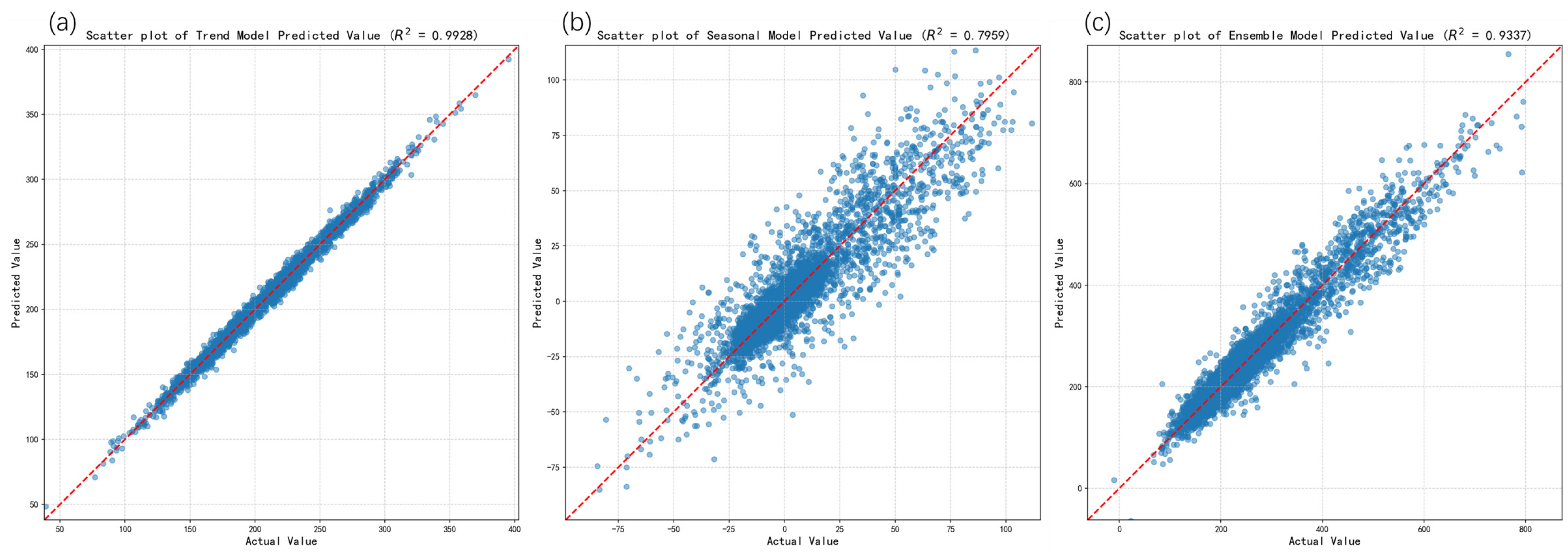
Figure 5 shows the independent prediction results of the model for the COD Trend and Seasonal components, as well as the final prediction result after reconstruction. Benefiting from the specialized “Long-term Dependency Attention” mechanism, the model achieved an extremely high goodness-of-fit ( R 2 = 0.99 ) in trend prediction.
For the frequently fluctuating seasonal component, the model utilized “Multi-scale Periodic Attention” to effectively extract diurnal variation patterns, achieving a good fit of R 2 = 0.80 .
This “divide and conquer” strategy has been widely proven effective in hybrid model research. Establishing dedicated prediction models for components of different frequencies can effectively avoid “mutual interference” when a single model processes multi-scale features, thereby achieving higher accuracy after reconstruction than a single model [36]. The final prediction result on the test set was R 2 = 0.93 The scatter points are tightly distributed on both sides of the diagonal line, verifying the superiority of this strategy in handling the non-linear dynamics of wastewater.
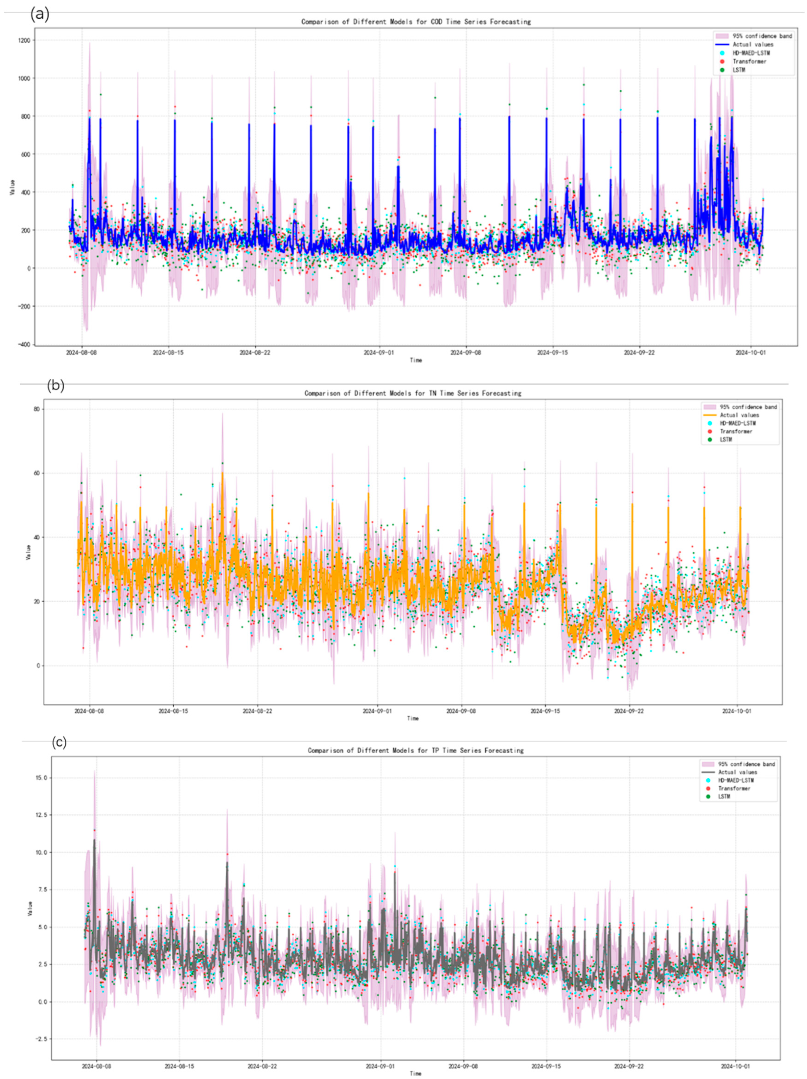
To verify the generalization ability of the model on different water quality parameters, we compared the time series prediction of HD-MAED-LSTM with mainstream baseline models (Transformer, LSTM) on three key indicators: COD, TN, and TP. In the COD prediction with the most severe fluctuations (Figure 6), traditional LSTM and Transformer models often exhibited significant lag or amplitude underestimation at the peaks (i.e., when shock loads occurred). This may be because conventional loss functions (such as MSE) tend to produce smooth averaged predictions, leading to a “peak-shaving” effect when the model faces sudden peaks [37].
In contrast, the prediction curve of the HD-MAED-LSTM model has the highest agreement with the ground truth, with the vast majority of prediction points falling precisely within the 95% Confidence Interval (CI). Introducing confidence interval evaluation is key to uncertainty quantification. A high-quality prediction model should not only pursue the accuracy of point prediction but also demonstrate the model’s robustness through narrow and high-coverage confidence intervals [38]. The sensitivity demonstrated by this model in capturing extreme points proves that its heterogeneous attention mechanism successfully overcame the smoothing bias of traditional models.
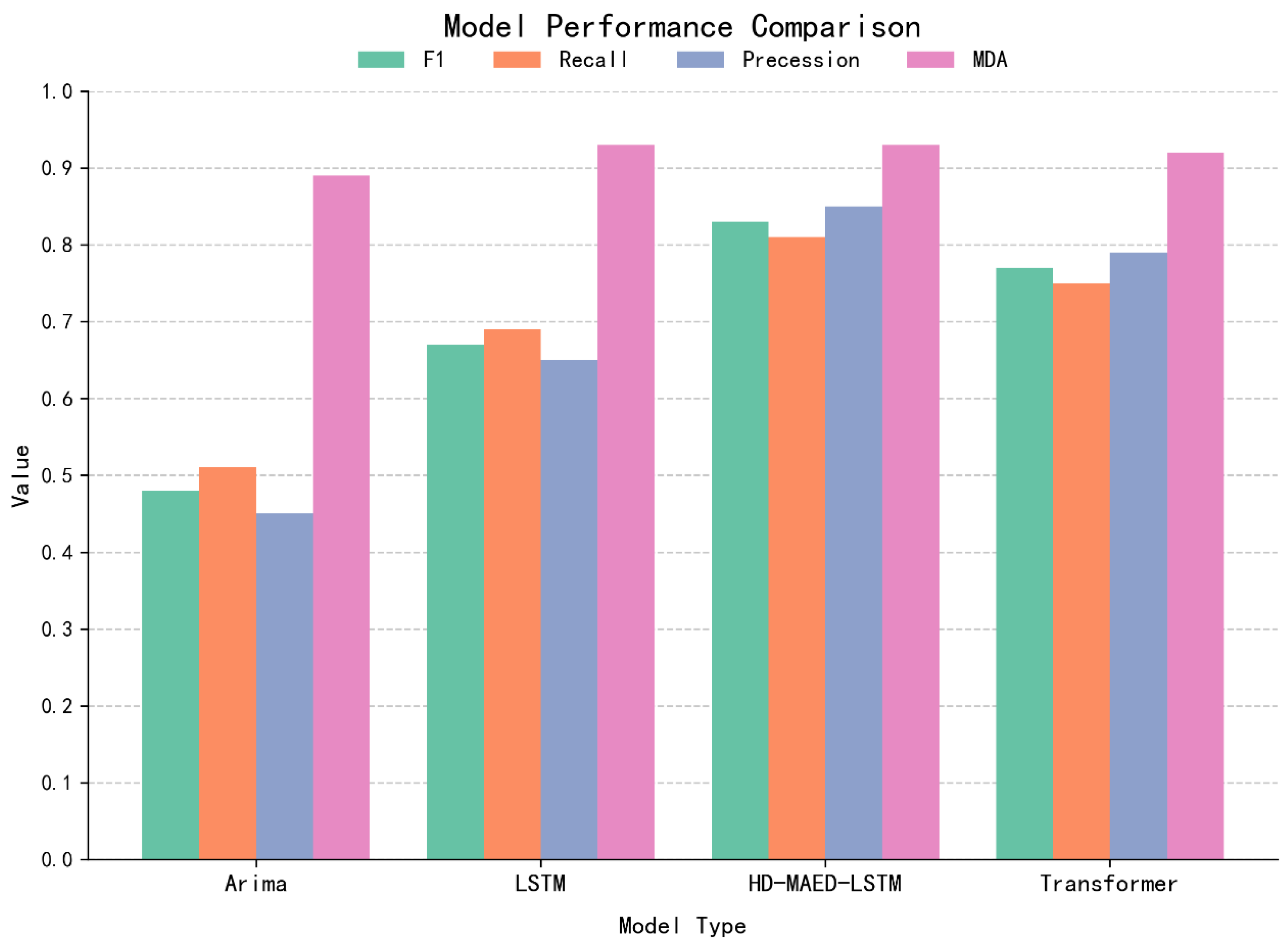
Focusing on the “high-concentration shock load” early warning capability of most concern to WWTPs, we compared the performance of each model on the binary classification warning metric (F1-Score) and the trend direction judgment metric (MDA) based on the COD test set data.
As shown in Figure 7, the traditional statistical model ARIMA performed the worst on all metrics due to its difficulty in capturing non-linear features. The HD-MAED-LSTM model achieved the highest F1-Score (0.83) in shock warning capability. This may be because when dealing with water quality anomaly detection tasks, deep learning networks integrated with attention mechanisms can more effectively identify sparse anomaly signals in the data, thereby achieving a better balance between Precision and Recall [39].
Furthermore, in terms of Mean Directional Accuracy (MDA), this model reached a high score of 0.93. In engineering control applications, the accuracy of the direction of change in the predicted value is often more important than the numerical error, as it directly determines the decision direction (e.g., “increase” or “decrease”) of the control system (such as aeration rate adjustment) [40]. The high MDA value of this model implies that it can provide highly reliable decision support for the “proactive pre-control” of WWTPs.

3.2. Contribution Analysis (Ablation Experiment)

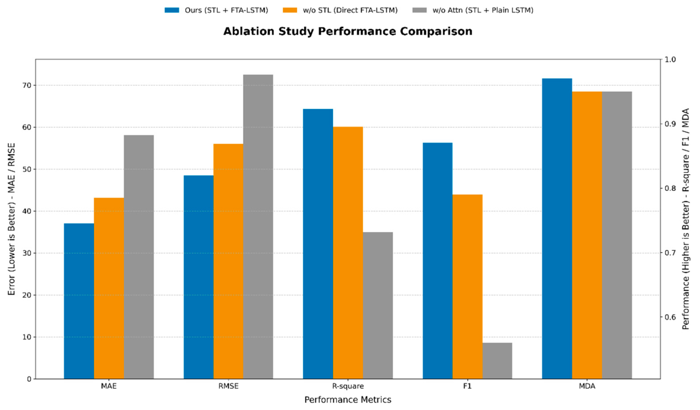
To quantitatively evaluate the effectiveness of each core component in the proposed model, ablation experiments were designed. The experimental setup included three comparison groups: the complete model (HD-MAED-LSTM), the model with the STL decomposition module removed (w/o STL), and the model with the specialized attention mechanism removed (STL + Plain LSTM). Figure 8 details the specific performance metrics of each variant model in the COD prediction task.
By comparing the performance of the complete model with the “w/o STL” model, the necessity of the signal decoupling strategy is clearly revealed. As shown in the figure, when the STL decomposition module is removed and the raw mixed sequence is directly input into the model, the prediction accuracy declines significantly: R 2 drops from 0.92 to 0.89, and RMSE rises from 48.46 to 56.04 (an increase of approximately 15.6%).
This result confirms the limitations of undecomposed models in modeling raw wastewater data with high-frequency fluctuations. Raw environmental data typically contain multi-scale non-stationary features. Forcing the neural network to simultaneously learn long-term trends and high-frequency noise through direct modeling can lead to convergence difficulties [41]. Through STL decomposition, the model transforms the complex raw sequence into three sub-sequences with relatively simple structures: trend, seasonal, and residual components. This aligns with the “Decomposition-Ensemble” paradigm proposed by Qiu et al. (2017) [42]. Their research found that this strategy can effectively reduce the “Sample Entropy” (SampEn) of the data itself, thereby significantly enhancing the interpretability and accuracy of the prediction model [42]. Therefore, the STL module in this study lays the foundation for high-precision feature extraction by reducing sequence complexity.
Comparing the experimental results of the complete model with the “w/o specialized attention mechanism (STL + Plain LSTM)” model reveals the core role of the HD-MAED attention module in capturing dynamic dependencies and identifying anomalous shocks. When the specialized attention LSTM was replaced by standard LSTM, the model performance experienced a precipitous drop: R 2 plunged to 0.73, and the MAE increased by 56.7% (from 37.08 to 58.12).
In terms of early warning metrics, the F1-Score of the standard LSTM model was only 0.56, far lower than the 0.83 of the proposed model. This phenomenon strongly proves the “information forgetting” defect of standard RNN architectures when processing long sequences. In long-sequence prediction research, although traditional LSTM introduces gating mechanisms, it struggles to distinguish the importance of different time steps when facing long input windows. It often assigns convergent weights to all historical information, causing key turning signals to be overwhelmed by noise [43].
The heterogeneous attention mechanism introduced in this paper can dynamically assign weights to historical time steps. After introducing the attention mechanism, the model can automatically focus on the “salient features” that are most strongly correlated with future moments, rather than blindly processing the entire sequence [44]. In this study, it is precisely this mechanism that enables HD-MAED-LSTM to keenly capture high-concentration shock signals from the residual component, thereby achieving a substantial improvement in F1-Score and ensuring the model’s robustness in coping with sudden pollution events.

3.3. Parameter Sensitivity Analysis

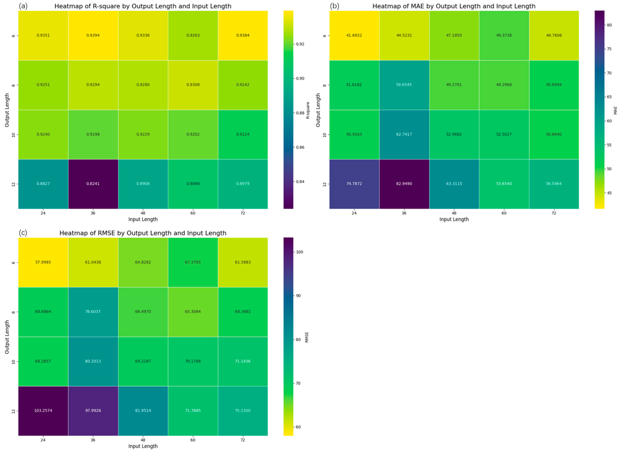
The input sequence length determines the amount of historical information available to the model, while the output sequence length represents the extent of the prediction into the future. Figure 9 presents heatmaps of model performance under different combinations of input lengths (24, 36, 48, 60, 72 h) and output lengths (6, 8, 10, 12 h).
The results of the error accumulation effect experiment in the prediction horizon show that regardless of the input length setting, model performance exhibits a monotonic downward trend as the prediction horizon increases. Taking the 48 h input as an example, when the prediction horizon increases from 6 h to 12 h, the RMSE rises significantly from 45.37 to 57.36, an increase of 26.4%. This phenomenon reflects the inherent characteristic of “temporal dependency decay” in time series prediction. Although this study adopted the One-shot prediction strategy to circumvent the error accumulation propagation associated with recursive prediction, the causal association and correlation between historical input information and far-future target variables inevitably weaken gradually as the prediction horizon extends. Furthermore, far-future states are often subject to more unforeseen random disturbances, increasing the difficulty for the model to extract effective features from historical sequences and establish precise mapping relationships, leading to a natural decline in the model’s inference capability for far-future states [45]. Based on the above analysis, to balance practicality and accuracy, this study selected 10 h as the prediction boundary.
Regarding the input sequence length in the “information-noise trade-off” of the input window, experiments revealed that the model does not always benefit from longer historical information. Experimental results show that the model performs best on the Output = 10 task when the input length is 24 h and 48 h (RMSE of 48.08 and 48.46, respectively). However, when the input length is set to 36 h or extended to 72 h, the prediction error actually increases (e.g., the RMSE for Input 36/Output 10 rises to 56.14).
This may be due to the “information-noise trade-off” phenomenon in deep learning modeling. Although a longer input length can provide more historical information, it may also introduce outdated information or redundant noise irrelevant to the current prediction target, thereby interfering with the model’s feature extraction weights. The selection of the input window should match the periodicity of the physical process [46]. Wastewater influent exhibits a significant 24-h diurnal cycle, so an input of 24 h or 48 h (containing 1–2 complete cycles) can maximize the effective information density. In contrast, a 36 h input window truncates the periodic pattern and introduces phase deviation, which explains the reason for its performance degradation.
To verify whether the proposed HD-MAED-LSTM framework is only applicable to specific data patterns, this study further evaluated the model’s generalization ability on different water quality prediction targets (COD, TN, TP). Different water quality parameters are controlled by distinct biochemical reaction kinetics and external disturbances, exhibiting vastly different statistical distribution characteristics.
Table 4 presents the statistical characteristics and model prediction performance of the three target variables. The Coefficient of Variation ( C V ) is commonly used as a key indicator to measure the fluctuation intensity and prediction difficulty of time series. A high CV value implies a dispersed data distribution, containing more random uncertainty caused by shock loads or measurement noise, which typically leads to a decrease in the goodness-of-fit ( R 2 ) of prediction models [47].
Among the datasets of the three target variables, COD exhibits the highest volatility ( C V = 0.7578 ) indicating that it is most severely affected by influent shocks; in contrast, the fluctuation of TN is relatively stable ( C V = 0.4428 ), showing strong regularity.
Despite the huge differences in the statistical characteristics of the input data, experimental results show that the model achieved excellent prediction accuracy ( R 2 > 0.91 ) on all three parameters.
For the high-volatility COD data ( C V = 0.7578 ), the model still maintained high accuracy ( R 2 = 0.9229 ). This may be because the STL decomposition strategy successfully decomposed the original high-frequency random fluctuations into a predictable trend component and a residual component requiring focused attention. This further verifies that the hybrid model architecture can effectively suppress random noise interference in high-variance data. For the relatively stable TN series, the model achieved the highest goodness-of-fit ( R 2 = 0.9315 ). This indicates that the model did not suffer from “overfitting” due to the complex attention mechanism and could keenly capture subtle trend changes in stable sequences.
The prediction performance of TP ( R 2 = 0.9133 ,   C V = 0.5916 ) falls between the two, showing a high consistency between performance and data complexity. As the volatility of the input data decreases (CV value drops from 0.7578 for the COD dataset to 0.4428 for TN), the prediction error (RMAE) also decreases from 17.03% to 13.81%. Overall, the HD-MAED-LSTM architecture is not overfitted to a specific data structure but possesses strong feature adaptability. This experiment confirms that the model can be applied to the precise prediction of multiple water quality parameters without modifying the core architecture, requiring only parameter fine-tuning.
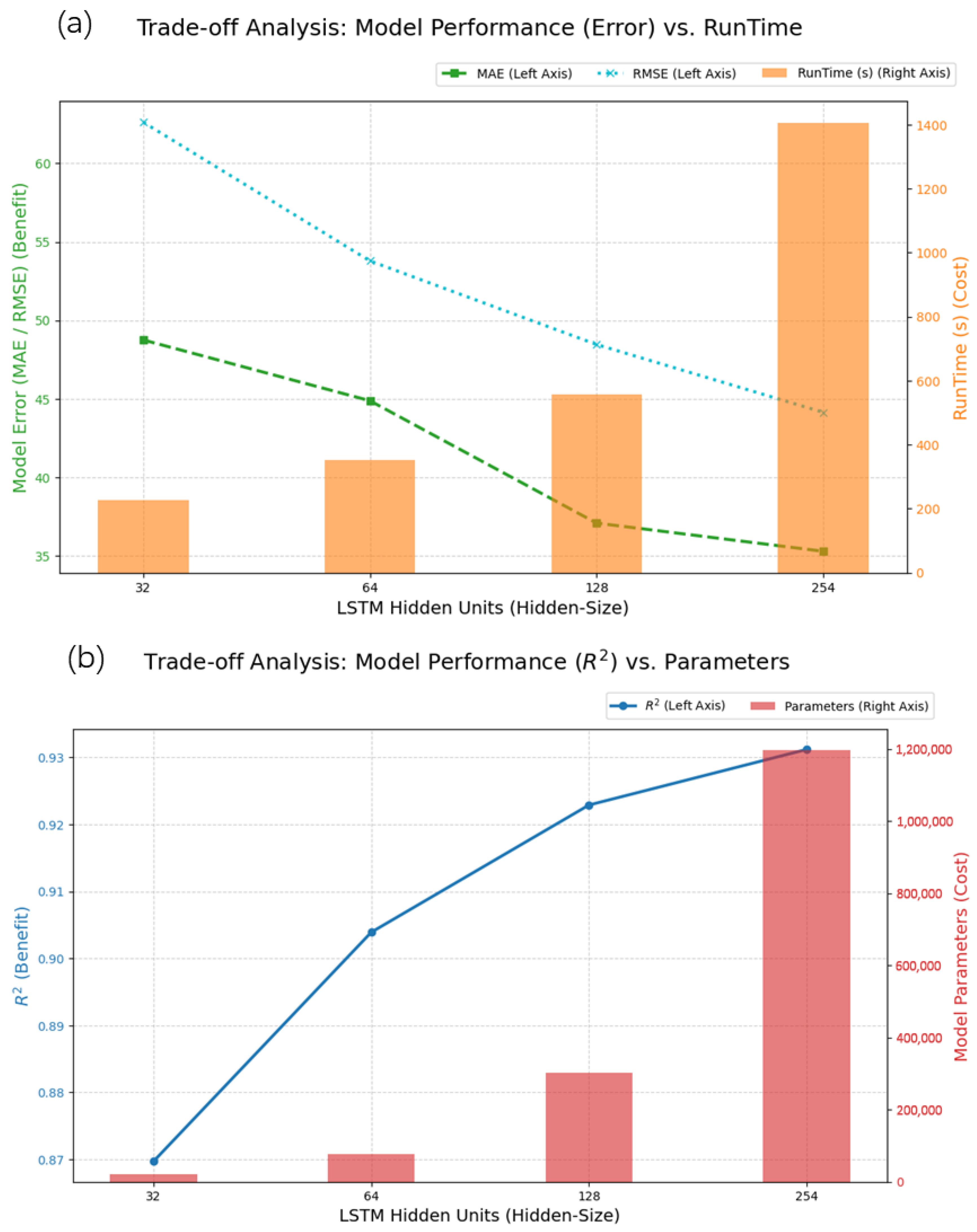
The number of LSTM hidden units directly determines the hypothesis space capacity and computational complexity of the model. Figure 10 presents the performance metrics and resource consumption of the model under different hidden unit configurations.
When the hidden units increased from 32 to 128, the model performance improved significantly, with RMSE decreasing from 62.62 to 48.46 and R 2 increasing from 0.8697 to 0.9229. This indicates that increasing the number of neurons effectively alleviated the underfitting problem. This phenomenon confirms that sufficient hidden neurons are a necessary condition for the model to capture non-linear dynamics and complex mapping relationships [48].
Model complexity is primarily quantified by two key metrics: the total volume of learnable parameters and the single-step inference time. As the number of hidden units increases, both the parameter count and the computational runtime exhibit a corresponding rise. This positive correlation is determined by the inherent structural characteristics of the LSTM network, where the dimension of the weight matrices in the gating mechanisms (forget, input, and output gates) scales quadratically with the hidden size. As shown in Figure 10, when the hidden units were further increased to 256, although the RMSE decreased slightly to 44.13 (an improvement of about 8.9%), the computational cost paid was enormous: the parameter count surged from 302 k to 1.19 M (an increase of about 3 times), and the training time extended from 556 s to 1404 s (an increase of about 1.5 times). In actual water engineering deployment, computational efficiency is a key constraint that cannot be ignored. Excessively pursuing minor accuracy improvements while ignoring the sharp increase in computational complexity will seriously hinder the application of the model in edge computing devices or real-time control systems.
Excessive model capacity also comes with the risk of overfitting. For water environment data with limited sample size, over-parameterized models tend to memorize training set noise rather than learning general laws. Considering that the 128-unit configuration achieved the best trade-off between performance ( R 2 = 0.92 ) and efficiency (RunTime < 10 min), and following the “Principle of Parsimony” (or Occam’s Razor) advocated by Ruan et al. (2023) [49], this study finally selected 128 as the optimal hidden layer size.

3.4. Discussion on Generalizability to Different WWTP Scenarios

Although this study validates the HD-MAED-LSTM model primarily on a complex industrial wastewater dataset, the proposed framework is designed with inherent generalizability to adapt to diverse WWTP configurations and operating conditions.
Regardless of the specific treatment process (e.g., A2/O, SBR, or Oxidation Ditch) or the influent source (domestic or industrial), water quality time series universally consist of three fundamental components: long-term trends, periodic variations, and stochastic fluctuations. By decoupling these components via STL, our model bypasses the complexity of specific physical constraints and focuses on the underlying mathematical structure of the data. Recent comparative studies have confirmed that such decomposition-based ensemble frameworks exhibit superior stability and generalizability across varying water quality datasets compared to monolithic models [50].
The proposed heterogeneous attention mechanism acts as a self-adaptive feature selector, capable of handling diverse influent characteristics ranging from domestic diurnal patterns to industrial shock loads. Recent studies have validated that attention-based architectures can effectively capture complex nonlinear relationships and long-range dependencies in sewage treatment data, outperforming static models in varying operational scenarios [51]. This structural flexibility ensures that the model can dynamically adjust its focus—prioritizing seasonal components in stable phases or residual anomalies during shock events—without requiring fundamental architectural redesign.
Furthermore, the high-dimensional feature representations learned by the HD-MAED-LSTM can serve as a robust foundation for Transfer Learning. As demonstrated by Wang et al. (2025), leveraging pre-trained models on scenario differences can significantly enable cross-task generalization across different water plants with limited data [52]. In future work, we aim to apply this strategy to fine-tune the proposed model on datasets from other WWTPs, thereby reducing the dependency on large-scale historical data for new deployments.

4. Conclusions and Future Work

This study addresses the critical time-scale mismatch in WWTPs by proposing the HD-MAED-LSTM framework. By adopting a “decompose-and-conquer” strategy, the model resolves the signal pollution issue inherent in traditional deep learning. It decouples non-stationary influent sequences into trend, seasonal, and residual components, applying specialized attention mechanisms to each.
Experimental results confirm the model’s superiority over baselines like LSTM and Transformer in predicting COD, TN, and TP. Notably, for shock load early warning, the model achieved an F1-Score of 0.83 and a Mean Directional Accuracy (MDA) of 0.93, effectively balancing process safety with proactive control. Ablation studies quantified the contribution of the specialized attention mechanism, which reduced the Mean Absolute Error (MAE) by 56.7%, proving it is the core driver of robustness.
Future work will focus on three directions: (1) verifying the framework’s generalization across diverse WWTP scales and processes; (2) integrating exogenous variables, such as rainfall and weather forecasts, to extend prediction horizons; and (3) coupling prediction results with control units (e.g., aeration systems) to construct a closed-loop system, quantitatively evaluating economic benefits like energy savings.

Supplementary Materials

The following supporting information can be downloaded at: https://www.mdpi.com/article/10.3390/w18030295/s1, Supplementary Materials S1; Supplementary Materials S2.

Author Contributions

Conceptualization, W.L. and J.H.; Data curation, W.L.; Formal analysis, W.L.; Funding acquisition, J.H. and F.Y.; Investigation, W.L.; Methodology, W.L. and Y.N.; Project administration, J.H. and Y.X.; Resources, J.H.; Software, W.L.; Supervision, J.H. and F.Y.; Validation, J.H.; Visualization, W.L.; Writing—original draft, W.L.; Writing—review & editing, J.H. and F.Y. All authors have read and agreed to the published version of the manuscript.

Funding

This research was funded by Shanghai Environmental Protection (Group) Co., Ltd. (SEPG) grant and the APC was funded by Fudan University.

Data Availability Statement

The data presented in this study are available in the article/Supplementary Material of this article. Further inquiries can be directed to the corresponding author.

Acknowledgments

We would like to thank the SEPG Company for providing financial support to this research.

Conflicts of Interest

Authors Fei Yuan and Yanjing Xu were employed by the company Shanghai Environmental Protection (Group) Co., Ltd. (SEPG). The remaining authors declare that the research was conducted in the absence of any commercial or financial relationships that could be construed as a potential conflict of interest. The authors declare that this study received funding from Shanghai Environmental Protection (Group) Co., Ltd. (SEPG). The funder was not involved in the study design, collection, analysis, interpretation of data, the writing of this article or the decision to submit it for publication.

References

  1. Xie, Y.; Wang, D.; Qiao, J. Dynamic Multi-Objective Intelligent Optimal Control toward Wastewater Treatment Processes. Sci. China Technol. Sci. 2022, 65, 569–580. [Google Scholar] [CrossRef]
  2. Wang, R.; Pan, Z.; Chen, Y.; Tan, Z.; Zhang, J. Influent Quality and Quantity Predictionin Wastewater Treatment Plant: Model Construction and Evaluation. Pol. J. Environ. Stud. 2021, 30, 4267–4276. [Google Scholar] [CrossRef]
  3. Faisal, M.; Muttaqi, K.M.; Sutanto, D.; Al-Shetwi, A.Q.; Ker, P.J.; Hannan, M.A. Control Technologies of Wastewater Treatment Plants: The State-of-the-Art, Current Challenges, and Future Directions. Renew. Sustain. Energy Rev. 2023, 181, 113324. [Google Scholar] [CrossRef]
  4. Jamaludin, M.; Tsai, Y.-C.; Lin, H.-T.; Huang, C.-Y.; Choi, W.; Chen, J.-G.; Sean, W.-Y. Modeling and Control Strategies for Energy Management in a Wastewater Center: A Review on Aeration. Energies 2024, 17, 3162. [Google Scholar] [CrossRef]
  5. Arismendy, L.; Cárdenas, C.; Gómez, D.; Maturana, A.; Mejía, R.; Quintero M., C.G. Intelligent System for the Predictive Analysis of an Industrial Wastewater Treatment Process. Sustainability 2020, 12, 6348. [Google Scholar] [CrossRef]
  6. Farhi, N.; Kohen, E.; Mamane, H.; Shavitt, Y. Prediction of Wastewater Treatment Quality Using LSTM Neural Network. Environ. Technol. Innov. 2021, 23, 101632. [Google Scholar] [CrossRef]
  7. Zhang, Y.; Li, C.; Jiang, Y.; Sun, L.; Zhao, R.; Yan, K.; Wang, W. Accurate Prediction of Water Quality in Urban Drainage Network with Integrated EMD-LSTM Model. J. Clean. Prod. 2022, 354, 131724. [Google Scholar] [CrossRef]
  8. Zhang, W.; Zhao, J.; Quan, P.; Wang, J.; Meng, X.; Li, Q. Prediction of Influent Wastewater Quality Based on Wavelet Transform and Residual LSTM. Appl. Soft Comput. 2023, 148, 110858. [Google Scholar] [CrossRef]
  9. Wang, S.; Yang, K.; Peng, H. Using a Seasonal and Trend Decomposition Algorithm to Improve Machine Learning Prediction of Inflow from the Yellow River, China, into the Sea. Front. Mar. Sci. 2025, 12, 1540912. [Google Scholar] [CrossRef]
  10. Xiao, Z.; Li, C.; Hao, H.; Liang, S.; Shen, Q.; Li, D. VBTCKN: A Time Series Forecasting Model Based on Variational Mode Decomposition with Two-Channel Cross-Attention Network. Symmetry 2025, 17, 1063. [Google Scholar] [CrossRef]
  11. Zhang, X.; Chang, X.; Li, M.; Roy-Chowdhury, A.; Chen, J.; Oymak, S. Selective Attention: Enhancing Transformer through Principled Context Control. arXiv 2024, arXiv:2411.12892. [Google Scholar] [CrossRef]
  12. Xie, Y.; Chen, Y.; Wei, Q.; Yin, H. A Hybrid Deep Learning Approach to Improve Real-Time Effluent Quality Prediction in Wastewater Treatment Plant. Water Res. 2024, 250, 121092. [Google Scholar] [CrossRef] [PubMed]
  13. Siddique, M.F.; Saleem, F.; Umar, M.; Kim, C.H.; Kim, J.-M. A Hybrid Deep Learning Approach for Bearing Fault Diagnosis Using Continuous Wavelet Transform and Attention-Enhanced Spatiotemporal Feature Extraction. Sensors 2025, 25, 2712. [Google Scholar] [CrossRef] [PubMed]
  14. Zare Abyaneh, H. Evaluation of Multivariate Linear Regression and Artificial Neural Networks in Prediction of Water Quality Parameters. J. Environ. Health Sci. Eng. 2014, 12, 40. [Google Scholar] [CrossRef]
  15. Manu, D.S.; Thalla, A.K. Artificial Intelligence Models for Predicting the Performance of Biological Wastewater Treatment Plant in the Removal of Kjeldahl Nitrogen from Wastewater. Appl. Water Sci. 2017, 7, 3783–3791. [Google Scholar] [CrossRef]
  16. Han, H.; Sun, M.; Han, H.; Wu, X.; Qiao, J. Univariate Imputation Method for Recovering Missing Data in Wastewater Treatment Process. Chin. J. Chem. Eng. 2023, 53, 201–210. [Google Scholar] [CrossRef]
  17. Zhang, Y.; Wang, J.; Li, C.; Duan, H.; Wang, W. Attention-Based Deep Learning Models for Predicting Anomalous Shock of Wastewater Treatment Plants. Water Res. 2025, 275, 123192. [Google Scholar] [CrossRef]
  18. Bagherzadeh, F.; Mehrani, M.-J.; Basirifard, M.; Roostaei, J. Comparative Study on Total Nitrogen Prediction in Wastewater Treatment Plant and Effect of Various Feature Selection Methods on Machine Learning Algorithms Performance. J. Water Process Eng. 2021, 41, 102033. [Google Scholar] [CrossRef]
  19. Barzegar, R.; Aalami, M.T.; Adamowski, J. Short-Term Water Quality Variable Prediction Using a Hybrid CNN–LSTM Deep Learning Model. Stoch. Environ. Res. Risk Assess. 2020, 34, 415–433. [Google Scholar] [CrossRef]
  20. Cleveland, R.B.; Cleveland, W.S.; Terpenning, I. STL: A Seasonal-Trend Decomposition Procedure Based on Loess. J. Off. Stat. 1990, 6, 3. [Google Scholar]
  21. Hochreiter, S.; Schmidhuber, J. Long Short-Term Memory. Neural Comput. 1997, 9, 1735–1780. [Google Scholar] [CrossRef]
  22. Cho, K.; Van Merrienboer, B.; Bahdanau, D.; Bengio, Y. On the Properties of Neural Machine Translation: Encoder–Decoder Approaches. In Proceedings of the SSST-8, Eighth Workshop on Syntax, Semantics and Structure in Statistical Translation, Doha, Qatar, 25 October 2014; Association for Computational Linguistics: Doha, Qatar, 2014; pp. 103–111. [Google Scholar]
  23. Sutskever, I.; Vinyals, O.; Le, Q.V. Sequence to Sequence Learning with Neural Networks. arXiv 2014, arXiv:1409.3215. [Google Scholar] [CrossRef]
  24. Bahdanau, D.; Cho, K.; Bengio, Y. Neural Machine Translation by Jointly Learning to Align and Translate. arXiv 2016, arXiv:1409.0473. [Google Scholar] [CrossRef]
  25. Vaswani, A.; Shazeer, N.; Parmar, N.; Uszkoreit, J.; Jones, L.; Gomez, A.N.; Kaiser, L.; Polosukhin, I. Attention Is All You Need. arXiv 2023, arXiv:1706.03762. [Google Scholar] [PubMed]
  26. Hao, J.; Liu, F. Improving Long-Term Multivariate Time Series Forecasting with a Seasonal-Trend Decomposition-Based 2-Dimensional Temporal Convolution Dense Network. Sci. Rep. 2024, 14, 1689. [Google Scholar] [CrossRef] [PubMed]
  27. Liu, Y.; Gong, C.; Yang, L.; Chen, Y. DSTP-RNN: A Dual-Stage Two-Phase Attention-Based Recurrent Neural Network for Long-Term and Multivariate Time Series Prediction. Expert Syst. Appl. 2020, 143, 113082. [Google Scholar] [CrossRef]
  28. Paszke, A.; Gross, S.; Massa, F.; Lerer, A.; Bradbury, J.; Chanan, G.; Killeen, T.; Lin, Z.; Gimelshein, N.; Antiga, L.; et al. PyTorch: An Imperative Style, High-Performance Deep Learning Library. arXiv 2019, arXiv:1912.01703. [Google Scholar]
  29. Zhang, G.P. Time Series Forecasting Using a Hybrid ARIMA and Neural Network Model. Neurocomputing 2003, 50, 159–175. [Google Scholar] [CrossRef]
  30. Hodson, T.O. Root-Mean-Square Error (RMSE) or Mean Absolute Error (MAE): When to Use Them or Not. Geosci. Model Dev. 2022, 15, 5481–5487. [Google Scholar] [CrossRef]
  31. Kingma, D.P.; Ba, J. Adam: A Method for Stochastic Optimization. arXiv 2017, arXiv:1412.6980. [Google Scholar] [CrossRef]
  32. Ahmed, U.; Mumtaz, R.; Anwar, H.; Shah, A.A.; Irfan, R.; García-Nieto, J. Efficient Water Quality Prediction Using Supervised Machine Learning. Water 2019, 11, 2210. [Google Scholar] [CrossRef]
  33. Wang, A.; Pianosi, F.; Wagener, T. Technical Report—Methods: A Diagnostic Approach to Analyze the Direction of Change in Model Outputs Based on Global Variations in the Model Inputs. Water Resour. Res. 2020, 56, e2020WR027153. [Google Scholar] [CrossRef]
  34. Kim, J.; Yu, J.; Kang, C.; Ryang, G.; Wei, Y.; Wang, X. A Novel Hybrid Water Quality Forecast Model Based on Real-Time Data Decomposition and Error Correction. Process Saf. Environ. Prot. 2022, 162, 553–565. [Google Scholar] [CrossRef]
  35. Chen, S.; Huang, J.; Wang, P.; Tang, X.; Zhang, Z. A Coupled Model to Improve River Water Quality Prediction towards Addressing Non-Stationarity and Data Limitation. Water Res. 2024, 248, 120895. [Google Scholar] [CrossRef] [PubMed]
  36. Liu, H.; Mi, X.; Li, Y. Smart Deep Learning Based Wind Speed Prediction Model Using Wavelet Packet Decomposition, Convolutional Neural Network and Convolutional Long Short Term Memory Network. Energy Convers. Manag. 2018, 166, 120–131. [Google Scholar] [CrossRef]
  37. Mistry, S.; Parekh, F. Flood Forecasting Using Artificial Neural Network. IOP Conf. Ser. Earth Environ. Sci. 2022, 1086, 012036. [Google Scholar] [CrossRef]
  38. Khosravi, A.; Nahavandi, S.; Creighton, D.; Atiya, A.F. Lower Upper Bound Estimation Method for Construction of Neural Network-Based Prediction Intervals. IEEE Trans. Neural Netw. 2011, 22, 337–346. [Google Scholar] [CrossRef]
  39. Grunova, D.; Bakratsi, V.; Vrochidou, E.; Papakostas, G.A. Machine Learning for Anomaly Detection in Industrial Environments. Eng. Proc. 2024, 70, 25. [Google Scholar]
  40. Kim, S.; Kim, H. A New Metric of Absolute Percentage Error for Intermittent Demand Forecasts. Int. J. Forecast. 2016, 32, 669–679. [Google Scholar] [CrossRef]
  41. Wang, X.; Liu, W.; Wang, Y.; Yang, G. A Hybrid NOx Emission Prediction Model Based on CEEMDAN and AM-LSTM. Fuel 2022, 310, 122486. [Google Scholar] [CrossRef]
  42. Qiu, X.; Ren, Y.; Suganthan, P.N.; Amaratunga, G.A.J. Empirical Mode Decomposition Based Ensemble Deep Learning for Load Demand Time Series Forecasting. Appl. Soft Comput. 2017, 54, 246–255. [Google Scholar] [CrossRef]
  43. Ran, X.; Shan, Z.; Fang, Y.; Lin, C. An LSTM-Based Method with Attention Mechanism for Travel Time Prediction. Sensors 2019, 19, 861. [Google Scholar] [CrossRef]
  44. Zou, X.; Zhao, J.; Zhao, D.; Sun, B.; He, Y.; Fuentes, S. Air Quality Prediction Based on a Spatiotemporal Attention Mechanism. Mob. Inf. Syst. 2021, 2021, 6630944. [Google Scholar] [CrossRef]
  45. Neagoe, A.; Tică, E.-I.; Vuță, L.-I.; Nedelcu, O.; Dumitran, G.-E.; Popa, B. Hybrid LSTM-ARIMA Model for Improving Multi-Step Inflow Forecasting in a Reservoir. Water 2025, 17, 3051. [Google Scholar] [CrossRef]
  46. Huan, J.; Zhang, C.; Xu, X.; Qian, Y.; Zhang, H.; Fan, Y.; Hu, Q.; Mao, Y.; Zhao, X. River Water Quality Forecasting: A Novel LSTM-Transformer Approach Enhanced by Multi-Source Data. Environ. Monit. Assess. 2025, 197, 1040. [Google Scholar] [CrossRef]
  47. Gazzaz, N.M.; Yusoff, M.K.; Aris, A.Z.; Juahir, H.; Ramli, M.F. Artificial Neural Network Modeling of the Water Quality Index for Kinta River (Malaysia) Using Water Quality Variables as Predictors. Mar. Pollut. Bull. 2012, 64, 2409–2420. [Google Scholar] [CrossRef]
  48. Sheela, K.G.; Deepa, S.N. Review on Methods to Fix Number of Hidden Neurons in Neural Networks. Math. Probl. Eng. 2013, 2013, 425740. [Google Scholar] [CrossRef]
  49. Ruan, J.; Cui, Y.; Meng, D.; Wang, J.; Song, Y.; Mao, Y. Integrated Prediction of Water Pollution and Risk Assessment of Water System Connectivity Based on Dynamic Model Average and Model Selection Criteria. PLoS ONE 2023, 18, e0287209. [Google Scholar] [CrossRef] [PubMed]
  50. Liu, T.; Liu, W.; Liu, Z.; Zhang, H.; Liu, W. Ensemble Water Quality Forecasting Based on Decomposition, Sub-Model Selection, and Adaptive Interval. Environ. Res. 2023, 237, 116938. [Google Scholar] [CrossRef] [PubMed]
  51. Zheng, J.; Suzuki, G.; Shioya, H. Sustainable Sewage Treatment Prediction Using Integrated KAN-LSTM with Multi-Head Attention. Sustainability 2025, 17, 4417. [Google Scholar] [CrossRef]
  52. Wang, Y.-Q.; Luo, X.-Q.; Zhou, H.-B.; Chen, J.-J.; Yin, W.-X.; Song, Y.-P.; Wang, H.-B.; Yu, B.; Tao, Y.; Wang, H.-C.; et al. Leveraging Scenario Differences for Cross-Task Generalization in Water Plant Transfer Machine Learning Models. Environ. Sci. Ecotechnol. 2025, 27, 100604. [Google Scholar] [CrossRef] [PubMed]
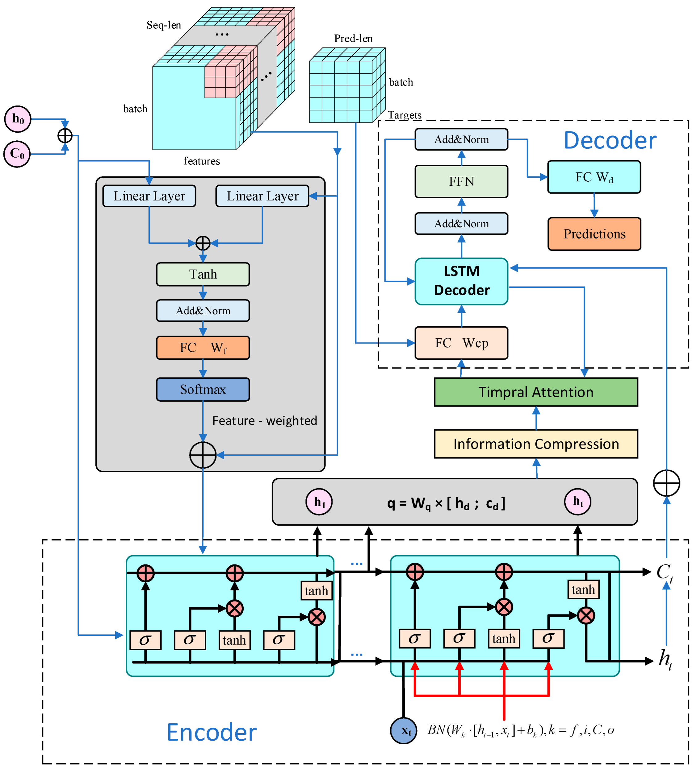
Figure 1. Multi-dimensional Attention Encoder-Decoder LSTM Prediction Model.
Water 18 00295 g001
Figure 2. Trend Long-term Dependency Attention.
Water 18 00295 g002
Figure 3. Seasonal Periodicity Attention.
Water 18 00295 g003
Figure 4. Residual Anomaly Detection Attention.
Water 18 00295 g004
Figure 5. Scatter plot of predicted versus actual COD values. (a) Trend Model Predicted Value. (b) Seasonal Model Predicted Value. (c) Ensemble Model Predicted Value.
Water 18 00295 g005
Figure 6. Time series forecasting comparison between HD-MAED-LSTM and baseline models for different prediction targets. (a) COD time series forecasting results. (b) TN time series forecasting results. (c) TP time series forecasting results.
Water 18 00295 g006
Figure 7. Comparison of shock load warning capabilities and directional accuracy among different models.
Water 18 00295 g007
Figure 8. Results of the ablation study quantifying the contributions of STL decomposition and specialized attention mechanisms.
Water 18 00295 g008
Figure 9. Heatmaps illustrating model performance under varying input and output sequence lengths. (a) Heatmap of R-square. (b) Heatmap of MAE. (c) Heatmap of RMSE.
Water 18 00295 g009
Figure 10. Rade-off analysis between model performance and computational cost. (a) Trade-off Analysis: Model Performance (Error) vs. Runtime. (b) Trade-off Analysis: Model Performance (R) vs. Parameters.
Water 18 00295 g010
Table 1. Descriptive statistics of the preprocessed time series dataset.
IndicatorUnitMinMaxMeanMedStd
pH - 6.74 10.91 7.27 7.26 0.22
COD mg/L 66.41 2841.00 217.73 169.70 165.00
NH3-N mg/L 0.24 78.91 24.68 23.98 9.24
TP mg/L 0.73 62.85 3.11 2.79 1.84
TN mg/L 6.92 98.32 33.87 32.12 15.00
Table 2. Model architecture configuration and training hyperparameters.
Model Architecture ParametersTraining Parameters
STL LOSS odd Epoch 500
STL Period 24 Optimizer Adam
Input Windows 48 Learning rate 0.001
Output Windows 10 Loss Function MSE-Loss
Hidden units 128 Early Stopping 20
Dropout Rate 0.3 Scheduler Patience 10
L2 Regularization e Scheduler Factor 0.5
Table 3. Statistical characteristics of the Trend and Seasonal components after STL decomposition.
IndicatorUnitMinMaxQ1Q2Q3Std
COD-Trend mg/L 88.86333.64136.32164.15213.2152.48
TN-Trend mg/L 9.7148.7828.4233.4037.437.14
TP-Trend mg/L 1.045.042.392.753.290.76
COD-Seasonal mg/L −96.91132.51−10.15−0.4615.3320.13
TN-Seasonal mg/L −15.3324.87−3.34−1.051.086.06
TP-Seasonal mg/L −1.473.17−0.35−0.130.160.60
Table 4. Comparison of data characteristics and model performance across different water quality targets.
TargetDataset CharacteristicsAbsolute PerformanceRelative Performance
ParamsStdCVR-squareMAERMSER-MAE
COD1650.75780.922937.077748.46010.1703
TN1.840.44280.93154.67916.94460.1381
TP150.59160.91330.48271.20110.1542
Disclaimer/Publisher’s Note: The statements, opinions and data contained in all publications are solely those of the individual author(s) and contributor(s) and not of MDPI and/or the editor(s). MDPI and/or the editor(s) disclaim responsibility for any injury to people or property resulting from any ideas, methods, instructions or products referred to in the content.