Multi-Scale and Interpretable Daily Runoff Forecasting with IEWT and ModernTCN

Abstract

Daily runoff series exhibit high complexity and significant fluctuations, which often lead to large prediction errors and limit the scientific basis of water resource scheduling and management. This study proposes a runoff prediction framework that incorporates upstream–downstream hydrological correlation information and integrates Improved Empirical Wavelet Transform (IEWT), SHAP-based interpretable feature selection, Improved Population-Based Training (IPBT), and the Modern Temporal Convolutional Network (ModernTCN) to enhance forecasting accuracy and model robustness. First, IEWT is employed to perform multi-scale decomposition of the daily runoff sequence, extracting structural features at different temporal scales. Then, upstream–downstream hydrological correlation information is introduced, and the SHAP method is used to evaluate the importance of multi-source basin features, eliminating redundant variables to improve input quality and training efficiency. Finally, IPBT is applied to optimize ModernTCN hyperparameters, thereby constructing a high-performance forecasting model. Case studies at the Hankou station demonstrate that the proposed IPBT-IEWT-SHAP-ModernTCN model significantly outperforms benchmark methods such as LSTM, iTransformer, and TCN in terms of accuracy, stability, and generalization. Specifically, the model achieves a root mean square error of 342.14, a mean absolute error of 251.01, and a Nash–Sutcliffe efficiency of 0.9992. These results indicate that the proposed method can effectively capture the nonlinear correlation characteristics between upstream and downstream hydrological processes, thus providing an efficient and widely adaptable framework for daily runoff prediction and scientific water resources management.

1. Introduction

Surface daily runoff is influenced by multiple factors, including precipitation, evapotranspiration, soil moisture, and topography, and exhibits highly complex and non-stationary characteristics. Accurate daily runoff prediction is of great significance for flood control and dispatching, water resources management, ecological conservation, and agricultural production. In recent years, traditional statistical and physically based hydrological models have been increasingly combined with data-driven approaches, and the rapid advancement of artificial intelligence (AI) techniques has further enhanced the accuracy and efficiency of hydrological forecasting [1,2]. However, operational daily forecasting still requires methods that are not only accurate but also robust and interpretable, so that model outputs can be trusted and acted upon in practice.

To address the limitations of single models in capturing the nonlinear and non-stationary characteristics of runoff series, signal decomposition techniques have been widely introduced as an effective preprocessing approach. Recent studies [3,4] have demonstrated that combining Complete Ensemble Empirical Mode Decomposition with Adaptive Noise (CEEMDAN) and improved optimization algorithms with deep learning architectures such as Temporal Convolutional Networks (TCN) and Transformer models can substantially enhance the accuracy of medium and long-term monthly runoff prediction, confirming the effectiveness of decomposition–optimization hybrid modeling strategies. Similarly, Wang et al. [5] employed Symplectic Geometric Mode Decomposition (SGMD) and Sample Entropy (SE) to filter subseries, and incorporated the African Vulture Optimization Algorithm (AVOA) to optimize an LSTM network, further improving prediction performance and highlighting the advantages of multi-technology integration for modeling complex hydrological sequences. In another study, Xiong et al. [6] proposed a secondary decomposition strategy (ELM + CEEMD + BiLSTM), which also verified that multi-level decomposition can effectively improve model performance. Moreover, Hu et al. [7] developed a two-layer optimization framework that integrates data decomposition techniques with multi-model combination strategies, establishing a closed-loop feedback mechanism between the decomposition and prediction processes to achieve dynamic performance optimization and continuous improvement. These hybrid pipelines have been widely evaluated across different forecasting horizons, and next-day daily runoff forecasting places particular emphasis on decomposition stability and boundary artifacts because unstable partitioning can degrade component quality and propagate errors to downstream prediction. In particular, the quality of decomposition may deteriorate for weakly periodic daily runoff, and unstable band partitioning can propagate errors to downstream predictors. These issues highlight the need for a more stable, multi-scale decomposition method that is tailored to daily runoff. This study addresses this need by proposing an improved EWT (IEWT) with cumulative-energy-based band partitioning and smoother transition filters.

Research based on machine learning and deep learning [8] has become increasingly abundant in recent years. Guo et al. [9] developed a hybrid HBV-XGBoost model that integrates hydrological simulation and machine learning to analyze runoff variations in the Xiangxi River Basin under changing climatic conditions. Yao et al. [10] incorporated the physical processes of the Xinnanjiang model hydrological model into deep learning models, including Gated Recurrent Unit (GRU) and its variants, and applied the integrated gradients method for interpretability analysis, achieving a significant improvement in daily runoff prediction accuracy. Li [11] proposed the SL-CNN-LSTM model, which integrates self-attention and local attention mechanisms into a CNN-LSTM framework for water temperature prediction Similarly, Tian et al. [12] and Wei et al. [13] developed decomposition–optimization hybrid frameworks by coupling mode decomposition methods (e.g., OVMD/VMD) with metaheuristic optimization algorithms and deep learning predictors (e.g., TCN-GRU or LSTM), achieving improved runoff forecasting accuracy across case studies. Liu et al. [14] introduced a GCNN-LSTM model combined with an IoT-based data acquisition system, which significantly enhanced river water level and runoff prediction performance. You et al. [15] developed a hybrid model integrating CNN, BiGRU, attention mechanisms, and optimization algorithms, designed for data-sparse regions, thereby improving model generalization and predictive stability. Qiao et al. [16] proposed a metaheuristic evolutionary deep learning framework, constructing a TCN-Improved Aquila Optimizer (IAO)-Random Forest (RF) hybrid model for rainfall-run off simulation and multi-step runoff prediction. Sun et al. [17] developed a short-term hybrid runoff prediction model combining the Long Short-Term Memory (LSTM) network, Improved Harris Hawks Optimization (IHHO) algorithm, and Optimal Variational Mode Decomposition (OVMD), which demonstrated high accuracy and stability in multi-step forecasting. Ma et al. [18] proposed an innovative runoff prediction framework integrating segmented decomposition sampling and multi-input neural networks. This framework, centered on Seasonal-Trend Decomposition using Loess (STL) and Convolutional Long Short-Term Memory (CNN-LSTM), performs temporal segmented decomposition to effectively avoid future information leakage while improving computational efficiency and predictive accuracy.

Recent advances in time-series forecasting have been driven by modern Transformer-based architectures, and these models are being increasingly explored for hydrological runoff/streamflow prediction. For instance, Transformer variants have been evaluated or adapted for streamflow/runoff forecasting using architectures such as Informer and Temporal Fusion Transformers (TFT). Hybrid and ensemble strategies have also been developed for hydrological time series, demonstrating the potential of these models to improve the accuracy and interpretability of water resources forecasting tasks [19,20,21,22]. Meanwhile, convolutional architectures remain competitive in hydrological forecasting, with TCN-based hybrids being used to balance short-term responsiveness with longer-term dependence in the context of complex hydrological dynamics [23]. Building on these developments, this study adopts ModernTCN: a recently proposed, modernized, pure-convolution backbone that enhances the effective receptive field and achieves strong performance across mainstream time-series tasks. This provides an efficient, robust alternative to Transformer-based forecasters for daily runoff prediction [24].

In addition, feature selection and model parameter optimization are equally critical for improving predictive performance. Tian et al. [25] integrated the Fisher Score and the Entropy Weight-TOPSIS method to identify key influencing factors, and further applied hyperparameter tuning, which significantly improved the short-term reservoir runoff forecasting accuracy. Similarly, Chen et al. [26] and Li et al. [27] employed Principal Component Analysis (PCA) for dimensionality reduction, in combination with Genetic Algorithm (GA) optimization of Backpropagation Neural Network (BP) models—both with and without wavelet analysis—to enhance annual runoff prediction precision. These studies collectively demonstrate that data preprocessing and algorithmic optimization play vital roles in boosting model performance and ensuring robust predictive capability. However, many conventional selection strategies (e.g., Fisher score, PCA) provide limited model-specific interpretability for multi-station inputs and do not explicitly quantify each upstream station’s contribution to the forecast. Moreover, hyperparameter tuning is often performed in a static or one-off manner, which may lead to unstable performance across changing hydrological regimes. These limitations motivate the use of SHAP-based attribution for transparent input screening and a dynamic population-based optimization strategy (IPBT) for robust ModernTCN configuration in this study.

Despite these advances, there are still several gaps in the forecasting of daily runoff in the context of operational water resources. Firstly, many decomposition–optimization hybrid studies focus on medium- and long-term (e.g., monthly) runoff prediction, whereas daily forecasting is required for flood dispatching, water regulation, and navigation management. In these areas, errors relating to rapid rises and peak flows can lead to significant risks in decision-making. Secondly, multi-station information is often incorporated in an ad hoc manner, with the dependency between upstream and downstream stations rarely being used transparently to eliminate redundant stations and features, which can introduce noise and reduce robustness. Thirdly, deep models used for daily runoff forecasting usually rely on manual or single-shot hyperparameter tuning, making it difficult to achieve consistent performance across different hydrological regimes. Finally, conventional spectrum-partitioning strategies in EWT can be unstable for daily runoff series with weak periodicity, reducing the quality of decomposition and subsequent predictions.

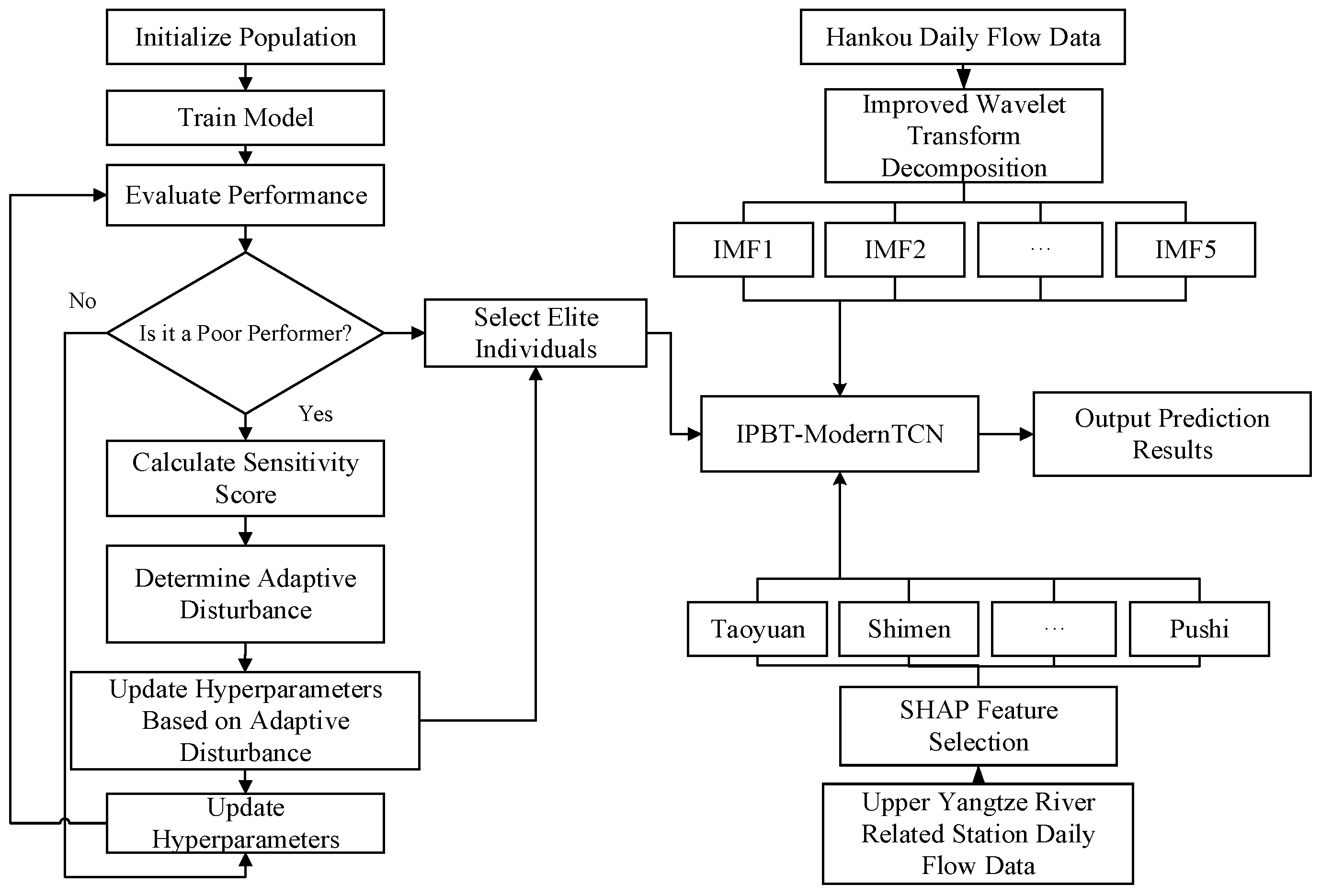
Inspired by advances in hybrid hydrological modeling and interpretable feature optimization, this study proposes an intelligent daily runoff prediction framework that integrates the Improved Empirical Wavelet Transform (IEWT), hydrological correlation analysis, SHAP-based feature selection, the Improved Population-Based Training (IPBT) algorithm, and the Modern Temporal Convolutional Network (ModernTCN) model. The main contributions of this work are summarized as follows:

(1)

Problem-oriented, multi-scale stabilization of daily runoff: We propose an improved EWT (IEWT) with a band partition based on cumulative energy and smoother filters. This improves the reliability of short-term forecasts used in operational water resources decision-making by obtaining stable components from highly non-stationary daily runoff series.

(2)

Interpretable upstream–downstream input selection: We integrate upstream–downstream hydrological dependence with SHAP-based interpretability to identify and retain the most influential upstream stations. This reduces redundant inputs and enhances the robustness and transparency of practical hydrological forecasting.

(3)

Robust automation of model configuration: We have developed an improved population-based training (IPBT) strategy with a decaying exploration factor, which dynamically optimizes the hyperparameters of the ModernTCN model. This yields stable performance under complex hydrological regimes without the need for heavy manual tuning.

(4)

Operationally relevant case study: Using the Hankou key control station in the Yangtze River Basin, we demonstrate that the proposed framework can support flood forecasting and water regulation tasks by providing an accurate prediction of the next day’s runoff.

The aim of this study is to improve the robustness and interpretability of next-day daily runoff forecasting for operational decision support. To this end, we have developed an integrated IPBT-IEWT-SHAP-ModernTCN framework that stabilizes daily runoff via IEWT decomposition, identifies influential upstream inputs using SHAP-based attribution, and enhances model configuration through IPBT-driven hyperparameter optimization. The Hankou case study shows that the proposed approach achieves substantial accuracy improvements over strong baselines and provides transparent input importance to support practical water resources applications.

2. Methods

2.1. Empirical Wavelet Transform Decomposition

Empirical Wavelet Transform (EWT) is an adaptive decomposition method for non-stationary signals. It partitions the signal’s Fourier spectrum and constructs an empirical wavelet filter bank for multi-scale decomposition [28]. EWT adaptively partitions the Fourier spectrum of the analyzed signal and constructs corresponding empirical wavelet functions to perform multi-scale decomposition. The general procedure of EWT consists of the following steps:

Step 1: Fourier Transform of the Daily Runoff Series $x(t)$:

EWT starts by analyzing the runoff signal in the frequency domain. For completeness, the continuous-time Fourier transform of $x(t)$ is written as Equation (1):

$$\hat{x}(\omega )={\int }_{-\infty }^{\infty }x(t)e^{-j\omega t}dt$$

(1)

where $\hat{x}(\omega )$ denotes the Fourier spectrum at angular frequency $\omega$.

Since daily runoff observations are finite-length, real-valued discrete-time sequences, the spectrum is computed in practice using the discrete Fourier transform (DFT), as given in Equation (2):

$${\hat{x}}_k=\sum _{n=0}^{N-1}{x}_n{e}^{-j2\pi kn/N}, k=0,\dots ,N-1$$

(2)

where $x_n$ denotes the daily runoff observation at the $n$-th time sample, ${\hat{x}}_k$ is the complex DFT coefficient at the $k$-th frequency bin, $N$ is the total number of samples in the runoff series, $j=\sqrt{-1}$ is the imaginary unit, and $k=0,\dots ,N-1$.

Step 2: Construction of Frequency Segmentation: The amplitude spectrum $|\hat{x}(\omega )|$ is plotted as the frequency spectrum. Using a smoothing or envelope method, $N-1$ frequency partition points ${\omega }_1,{\omega }_2,\dots ,{\omega }_{N-1}$ are adaptively identified. The entire spectrum domain $\mathsf{\Omega }=\{{\omega }_0=0,{\omega }_1,\dots ,{\omega }_N=\pi \}$ is divided into N sub-bands, where each frequency band is defined as: ${\mathsf{\Lambda }}_n=[{\omega }_{n-1},{\omega }_n], n=1,2,\dots ,N$.

Step 3: Construction of the Empirical Wavelet Filter Bank, a smooth transition function $\theta (x)$ introduced to design both low-pass and band-pass filters in the frequency domain. It is defined as Equation (3):

$$\theta (x)=\left\{\begin{array}{cc}\hfill 0,\hfill & x\le 0\hfill \\ \sin \left({\displaystyle \frac{\pi }{2}}x\right),& 0<x<1\hfill \\ 1,& x\ge 1\hfill \end{array}\right.$$

(3)

where $x$ is a normalized argument used to control the smooth connection between adjacent passbands; $\theta (x)=0$ and $\theta (x)=1$ enforce flat responses outside the transition interval, and the sinusoidal segment provides a continuous transition for $0<x<1$.

Then, using the band boundaries ${\omega }_n$ obtained in Step 2, the $n$-th empirical wavelet filter ${\hat{\varphi }}_n(\omega )$ is constructed as Equation (4):

$${\hat{\varphi }}_n(\omega )=\left\{\begin{array}{cc}1,& \omega \in [{\omega }_{n-1}+\tau ,{\omega }_n-\tau ]\hfill \\ \theta \left({\displaystyle \frac{\omega -({\omega }_n-\tau )}{\tau }}\right),& \omega \in [{\omega }_n-\tau ,{\omega }_n+\tau ]\hfill \\ \theta \left({\displaystyle \frac{({\omega }_{n-1}+\tau )-\omega }{\tau }}\right),& \omega \in [{\omega }_{n-1}-\tau ,{\omega }_{n-1}+\tau ]\hfill \\ 0,& \mathrm{oterwise}\hfill \end{array}\right.$$

(4)

where $\omega$ denotes the angular frequency, ${\omega }_n$ are the frequency-band boundaries, and $\tau >0$ controls the bandwidth of the transition region around each boundary (i.e., it determines how gradually the filter response changes near ${\omega }_{n-1}$ and ${\omega }_n$). The “otherwise” case ensures that ${\hat{\varphi }}_n(\omega )$ has compact support outside the designated band and its transition neighborhoods.

Step 4: Frequency-Domain Filtering. The filtered representation of each sub-band signal is obtained by applying the empirical wavelet filters to the Fourier-transformed signal, is written as Equation (5):

$${\hat{x}}_n(\omega )=\hat{x}(\omega )\cdot {\hat{\varphi }}_n(\omega )$$

(5)

where ${\hat{x}}_n(\omega )$ is the Fourier spectrum of the original runoff series $x(t)$, and ${\hat{x}}_n(\omega )$ denotes the spectrum of the $n$-th filtered sub-band.

Step 5: Inverse Fourier Transform for IMF Reconstruction: Each Intrinsic Mode Function (IMF) is recovered through the inverse Fourier transform as follows:

$$x_n(t)={\displaystyle \frac{1}{2\pi }}{\int }_{-\pi }^{\pi }{\hat{x}}_n(\omega )e^{j\omega t}d\omega$$

(6)

where $j=\sqrt{-1}$, and $x_n(t)$ is the reconstructed $n$-th IMF corresponding to the $n$-th frequency band.

Final Signal Reconstruction: The original runoff signal can be reconstructed by summing all decomposed IMFs:

$$x(t)=\sum _{n=1}^N{x}_n(t)$$

(7)

Through the above steps, the daily runoff series $x(t)$ of the Hankou Hydrological Station is successfully decomposed into N IMFs, with each IMF representing the flow variation characteristics at a distinct frequency scale.

2.2. Improved Empirical Wavelet Transform

The standard Empirical Wavelet Transform (EWT) may encounter several issues when processing hydrological signals characterized by weak periodicity or ambiguous seasonal patterns: (1) Unstable spectral extrema, which lead to inaccurate band segmentation; (2) Overly sharp filter transitions, which may cause frequency leakage between adjacent sub-bands. To address these problems, two improvements are proposed in this study for the decomposition of daily runoff data.

Improvement 1: Frequency Band Division Based on Cumulative Energy:

Given the Fourier spectrum $\hat{x}(\omega )$, the power spectral density is defined as shown in Equation (8):

$$P(\omega )=|\hat{x}(\omega ){|}^2$$

(8)

where $P(\omega )$ denotes the spectral energy distribution at angular frequency $\omega$.

The cumulative energy function is then computed according to Equation (9):

$$C(\omega )={\int }_0^{\omega }P(\xi )d\xi$$

(9)

where $C(\omega )$ represents the accumulated spectral energy from 0 to $\omega$, and $\xi$ is the integration variable.

To obtain stable frequency boundaries, the total energy $C(\pi )$ is evenly divided into $N$ segments as specified in Equation (10):

$$C({\omega }_k)={\displaystyle \frac{k}{N}}C(\pi ), k=1,2,\dots ,N-1$$

(10)

where ${\omega }_k$ are the resulting boundary frequencies, and $N$ is the number of sub-bands. This cumulative-energy-based segmentation reduces sensitivity to spurious local extrema in the spectrum, making it more suitable for daily runoff sequences with weak periodicity and strong non-stationarity.

This approach enables stable determination of frequency boundaries ${\omega }_k$, making it more suitable for runoff sequences with weak periodicity and poor stationarity.

Improvement 2: High-Order Smooth Filter Design:

To smooth the filter response across the overlap region at band boundaries and reduce boundary artifacts in the decomposed components, a hyperbolic tangent function is introduced to replace the original smooth transition function, as defined in Equation (11):

$$\theta (x): \theta (x)={\displaystyle \frac{1}{2}}\left[1+\tanh \left({\displaystyle \frac{x-0.5}{ϵ}}\right)\right]$$

(11)

where $x$ is the normalized transition argument and $\epsilon >0$ controls the smoothness (i.e., the steepness) of the transition.

With the above modification, the improved empirical wavelet filters operate similarly to those in standard EWT. The frequency-domain filtering process is performed as shown in Equation (12):

$${\hat{x}}_n(\omega )=\hat{x}(\omega )\cdot {\hat{\varphi }}_n^{change}(\omega )$$

(12)

where $\hat{x}(\omega )$ is the Fourier spectrum of the original signal, ${\hat{\varphi }}_n^{change}$ denotes the improved empirical wavelet filter for the $n$-th band, and ${\hat{x}}_n(\omega )$ is the filtered spectrum associated with the $n$-th component.

Each component is recovered through the inverse Fourier transform given in Equation (13):

$$x_n(t)={\displaystyle \frac{1}{2\pi }}{\int }_{-\pi }^{\pi }{\hat{x}}_n(\omega )e^{j\omega t}d\omega$$

(13)

where $x_n\left(t\right)$ denotes the reconstructed $n$-th component in the time domain.

Finally, the original signal is reconstructed by summing all components as expressed in Equation (14):

$$x(t)=\sum _{n=1}^N{x}_n(t)$$

(14)

where $x(t)$ is the original daily runoff signal and $N$ is the number of decomposed components.

Through these improvements, the proposed Improved EWT (IEWT) achieves smoother filter transitions and more stable frequency segmentation, making it more effective for analyzing the non-stationary and weakly periodic characteristics of daily runoff series.

2.3. Population-Based Training (PBT) Algorithm

The Population-Based Training (PBT) algorithm is an evolutionary optimization strategy that integrates hyperparameter optimization with model weight training. It was first proposed by DeepMind and later implemented on the Neural Network Intelligence (NNI) platform [29]. In this framework, each individual model in the population evolves dynamically through evaluation, replication, and perturbation to maximize final model performance. Let the population size be $\mathrm{N}$, For the $i\mathrm{-th}$ individual, the hyperparameter vector is defined as shown in Equation (15):

$$h_i=\left(h_i^{(1)},h_i^{(2)},h_i^{(3)},h_i^{(4)},h_i^{(5)},h_i^{(6)}\right)$$

(15)

Each dimension corresponds to a specific hyperparameter as follows: $h_i^{(1)}$-batch_size, $h_i^{(2)}$-train_epochs, $h_i^{(3)}$-dropout, $h_i^{(4)}$-d_ff, $h_i^{(5)}$-d_model, $h_i^{(6)}$-learning_rate. These hyperparameters are dynamically evaluated, replicated, and perturbed throughout the PBT process to achieve continuous optimization.

Step 1: Population Initialization

At the beginning of PBT, a population of $N$ individuals is initialized. The initial population is constructed as specified in Equation (16):

$$P^0=\left\{({\theta }_i^0,h_i^0)\mid i=1,2,\dots N\right\}$$

(16)

where ${\theta }_i^0$ represents the initial model weights, and is randomly sampled from a predefined hyperparameter space ${\mathcal{U}}_h$.

Step 2: Model Training Process

Each individual model is trained independently for a fixed training interval (or a fixed number of epochs), denoted by $\mathsf{\Delta }t$. The weight update over one training cycle follows Equation (17):

$${\theta }_i^t=\mathcal{M}(h_i^{t-\mathsf{\Delta }t};{\theta }_i^{t-\mathsf{\Delta }t})$$

(17)

where $\mathcal{M}$ represents the training function controlled by hyperparameters $h_i$, and $\mathsf{\Delta }t$ denotes the duration of each training cycle or epoch count.

Step 3: Performance Evaluation: After each training cycle, the performance of each individual is evaluated on a validation set using a fitness function, as given in Equation (18):

$$f_i^t=f({\theta }_i^t,h_i^t)$$

(18)

where $f_i^t$ represents the fitness value of the $i\mathrm{-th}$ individual, with smaller values indicating better performance.

Step 4: Selection and Evolution Mechanism (Core Process)

If the performance of an individual is relatively poor (e.g., ranked in the bottom 20% of the population), an exploit-explore strategy is triggered to enhance evolutionary optimization:

(a) Exploit—Replication of Elite Individuals: An elite individual $j$ is randomly selected from the top 20% of the population, and its parameters and hyperparameters are copied to the underperforming individual $i$, as shown in Equation (19):

$${\theta }_i^t\leftarrow {\theta }_j^t, h_i^t\leftarrow h_j^t$$

(19)

where ${\theta }_i^t$ and ${\theta }_j^t$ denote the model weights of individuals $i$ and $j$ at cycle $t$, respectively, and $h_i^t$ and $h_j^t$ are their corresponding hyperparameter vectors. This replication step allows poorly performing individuals to inherit strong configurations without restarting training.

(b) Explore—Perturbation of Hyperparameters: To further explore the search space and avoid premature convergence, small random perturbations are introduced to the copied hyperparameters. The perturbation rule is defined in Equation (20):

$$h_i^{(k)}\leftarrow h_j^{(k)}\cdot {\gamma }_i^{(k)}, {\gamma }_i^{(k)}\sim \mathrm{Uniform}(1-ϵ,1+ϵ)$$

(20)

where ${\gamma }_i^{(k)}$ denotes the perturbation coefficient for the $k\mathrm{-th}$ hyperparameter, and $ϵ$ controls the magnitude of the perturbation.

The core mechanism of the PBT algorithm combines local exploitation with global exploration, enabling continuous co-evolution of model weights and hyperparameters throughout dynamic training. This strategy allows the model to maintain both optimization efficiency and search diversity, resulting in superior convergence stability and performance robustness.

2.4. Improved Algorithm Based on Population-Based Training (PBT)

In the original PBT framework, uniform perturbations are applied to all hyperparameters during the exploration phase. However, this may lead to unstable convergence or cause the algorithm to jump out of the optimal region due to excessive randomness in later training stages. To address this issue, a dynamic exploration factor ${ϵ}_t$ is introduced. This factor gradually reduces the perturbation amplitude as the training progresses, preventing excessive perturbation in the later stages of model optimization.

Dynamic Exploration Factor: Let the total number of training steps be $T$, the current training step be $t(t=0,1,\dots ,T)$, the initial perturbation amplitude be ${\epsilon }_0$, and the decay-rate coefficient be $\alpha >0$. Then, the dynamic exploration factor ${\epsilon }_t$ is defined as follows:

$${\epsilon }_t={\epsilon }_0{\left(1-{\displaystyle \frac{t}{T}}\right)}^{\alpha }$$

(21)

where ${\epsilon }_t$ denotes the exploration intensity at step $t$, ${\epsilon }_0$ is the initial exploration magnitude, $T$ is the maximum number of training steps (or total training cycles), and $\alpha$ controls the decay speed of exploration. This schedule enables broader exploration in early training stages and increasingly refined search near convergence.

This adaptive design allows the algorithm to gradually decrease the exploration intensity as training approaches convergence, thereby achieving a balance between exploration and exploitation.

Perturbation Strategy: During the Explore phase, for the $k$-th hyperparameter copied from the elite individual j, the perturbation is applied as follows:

$$h_i^{(k)}\leftarrow h_j^{(k)}\cdot {\gamma }_i^{(k)}, {\gamma }_i^{(k)}\sim \mathrm{Uniform}(1-{\epsilon }_t,1+{\epsilon }_t)$$

(22)

where ${\gamma }_i^{(k)}$ denotes the random perturbation coefficient and $h_i^{(k)}$ represents the $k$-th hyperparameter of the i-th individual.

Through this dynamic perturbation mechanism, the improved PBT algorithm (IPBT) enables adaptive exploration control—promoting broader search in early stages and refined optimization later. Consequently, IPBT effectively enhances training stability, convergence efficiency, and the generalization ability of the optimized model.

2.5. SHAP-Based Feature Selection

In the context of daily runoff prediction, the model typically involves multiple hydrological stations and a variety of input features such as water level and runoff observations. However, the excessive number of features often leads to increased model complexity, amplified noise interference, and reduced interpretability. To address these issues, the SHAP (SHapley Additive exPlanations) method is introduced to quantify the contribution of each input feature to the model’s predictive output, thereby identifying the most influential features that govern runoff dynamics.

Definition and Calculation of SHAP Values: The SHAP value originates from the Shapley value concept in cooperative game theory. It measures the marginal contribution of each feature to the overall model output, satisfying key mathematical properties such as fairness, rationality, and additivity [30].

Let the input feature vector be defined as: $x=(x^{(1)},x^{(2)},\dots ,x^{(M)})$ where M denotes the total number of input features, and the prediction model is represented as $f(x)\in ℝ$, The model output is denoted by $y=f(x)$. Let $S\subseteq \{1,2,\dots ,M\}$.

The mathematical definition of the SHAP value is given as follows. Let $S$ represent a subset of features, and for the $j\mathrm{-th}$ feature $x(j)$, its SHAP value is mathematically defined as:

$${\varphi }^{(j)}=\sum _{S\subseteq \mathcal{F}\setminus \left\{j\right\}}{\displaystyle \frac{\left|S\right|!(M-|S|-1)!}{M!}}\left[\begin{array}{c}{f}_{S\cup \left\{j\right\}}(x)-f_S(x)\end{array}\right]$$

(23)

where $M$ is the total number of input features, ${\varphi }^{(j)}$ denotes the SHAP value of the $j$-th. $f_S(x)$ and $f_{S\cup \left\{j\right\}}(x)$ represent the model outputs based on subsets $S$ and $S\cup \left\{j\right\}$, respectively.

Step 1: Construction of the Daily Runoff Prediction Model Using the TCN: To establish a complete mapping relationship between hydrological features and runoff sequences (e.g., at the Hankou Station), the Temporal Convolutional Network (TCN) is first employed for daily runoff prediction. This model provides a foundational framework for subsequent SHAP-based interpretability analysis.

Input Definition: Let the model input be a multivariate time-series feature matrix with a time window length of $L$ and feature dimension $\mathrm{M}$. The input matrix $X_t$ is defined as:

$$X_t=\left[\begin{array}{cccc}{x}_t^{(1)}& x_{t-1}^{(1)}& \dots & x_{t-L+1}^{(1)}\\ x_t^{(2)}& x_{t-1}^{(2)}& \dots & x_{t-L+1}^{(2)}\\ ⋮& ⋮& \ddots & ⋮\\ x_t^{(M)}& x_{t-1}^{(M)}& \dots & x_{t-L+1}^{(M)}\end{array}\right]\in {ℝ}^{M\times L}$$

(24)

where $x_t^{(j)}$ is the value of the $j\mathrm{-th}$ feature at time $t$.

Model Definition: The Temporal Convolutional Network (TCN) [31] maps the multivariate input sequence to a single-step prediction target, the runoff on day $t+1$:

$${\hat{y}}_{t+1}=f_{\mathrm{TCN}}(X_t;\Theta )$$

(25)

where ${\hat{y}}_{t+1}$ is the predicted daily runoff, $\Theta$ denotes the set of model parameters (including convolutional weights, biases, and dropout rates), and $f_{\mathrm{TCN}}$ represents the TCN model, which consists of stacked dilated causal 1D convolutional layers.

The model is trained by minimizing the mean squared error (MSE) loss function:

$${\mathcal{L}}_{\mathrm{MSE}}={\displaystyle \frac{1}{N}}\sum _{t=1}^N{\left(y_{t+1}-{\hat{y}}_{t+1}\right)}^2$$

(26)

where $y_{t+1}$ represents the true runoff value on day $t+1$, $N$ is the total number of samples generated by the sliding window.

Model Optimization: The optimal model parameters are obtained through gradient-based optimization:

$${\Theta }^{\ast }=\arg \underset{\Theta }{\min }{\mathcal{L}}_{\mathrm{MSE}}(\Theta )$$

(27)

After training convergence, the final model $f_{\mathrm{TCN}}(X_t;{\Theta }^{\ast })$, is retained for SHAP-based feature attribution analysis, which evaluates the contribution of each input feature to the predicted runoff (i.e., the daily discharge at Hankou Station).

Step 2: Calculation of SHAP values for each sample, For each sample $x_i$, the SHAP value of its $j\mathrm{-th}$ feature is computed as: ${\varphi }_i^{(j)}=\mathrm{SHAP}(x_i^{(j)})$.

After computing SHAP values for all samples and all features, they are organized into a SHAP value matrix as shown in Equation (28):

$$\mathsf{\Phi }=\left[\begin{array}{cccc}{\varphi }_1^{(1)}& {\varphi }_1^{(2)}& \dots & {\varphi }_1^{(M)}\\ {\varphi }_2^{(1)}& {\varphi }_2^{(2)}& \dots & {\varphi }_2^{(M)}\\ ⋮& ⋮& \ddots & ⋮\\ {\varphi }_N^{(1)}& {\varphi }_N^{(2)}& \dots & {\varphi }_N^{(M)}\end{array}\right]$$

(28)

where $N$ denotes the total number of samples, and $M$ represents the number of input features, and ${\varphi }_i^{(j)}$ is the SHAP attribution assigned to feature $j$ for sample $i$.

Step 3: Aggregation of SHAP Importance Scores

To evaluate the overall importance of each feature across all samples, the SHAP values are aggregated as follows:

$${\overline{\varphi }}^{(j)}={\displaystyle \frac{1}{N}}\sum _{i=1}^N\left|{\varphi }_i^{(j)}\right|$$

(29)

where ${\overline{\varphi }}^{(j)}$ denotes the global importance score of feature $j$, and the absolute value $\left|{\varphi }_i^{(j)}\right|$ prevents positive and negative contributions from canceling out.

Based on these aggregated scores, the feature-importance vector is constructed as shown in Equation (30):

$$\overline{\varphi }=\left({\overline{\varphi }}^{(1)},{\overline{\varphi }}^{(2)},\dots ,{\overline{\varphi }}^{(M)}\right)$$

(30)

where $\varphi \in {ℝ}^M$ summarizes the global SHAP importance of all input features.

Step 4: Feature Selection and Reconstruction: Based on the aggregated importance scores, the top $K$ most influential features are selected according to either a predefined threshold or by ranking the highest SHAP values. The selected feature index set is denoted as in Equation (31):

$${\mathcal{F}}^{\ast }={\mathrm{TopK}}_j\left(\overline{\varphi }(j)\right)$$

(31)

where ${\mathcal{F}}^{\ast }\subseteq \{1,2,\dots ,M\}$ contains the indices of the $K$ features with the largest values of $\left(\overline{\varphi }(j)\right)$, and ${\mathrm{TopK}}_j$ eturns the corresponding feature indices.

Accordingly, the final feature set used for model construction is represented as in Equation (32):

$$x^{\ast }=\{x^{(j)}\mid j\in {\mathcal{F}}^{\ast }\}$$

(32)

where $x^{\ast }$ denotes the reduced input feature set consisting only of the selected predictors.

This feature selection strategy ensures that only the most informative and relevant predictors are retained, effectively reducing data redundancy while maintaining strong explanatory power and model interpretability.

2.6. ModernTCN Time-Series Model

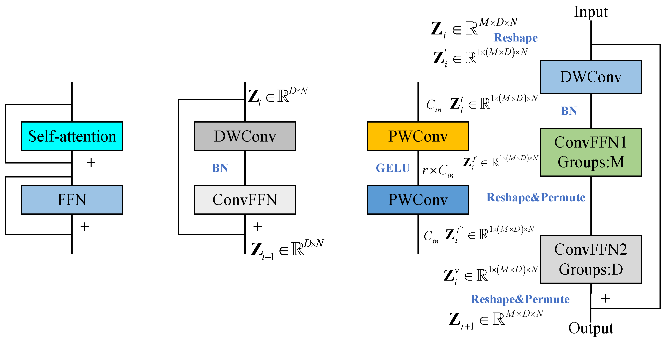
The ModernTCN model is a modernized fully convolutional architecture specifically designed for time-series analysis. It enhances the receptive field and computational efficiency of convolutional operations by introducing large convolution kernels and a decoupled design of depthwise-separable convolutions. Figure 1 and Figure 2 illustrate the overall framework of the ModernTCN model and the corresponding runoff-forecasting process [24]. In this study, the model input consists of hydrological and runoff data from upstream stations over the past 48 days, with 9 variables in total. The model output is the predicted daily runoff for the next day.

To preserve the dimensional independence of variables and prevent information leakage, each hydrological variable is first independently divided into local patches and embedded separately. Input Definition:

Step 1: Input Definition and Embedding. The multivariate input sequence is defined as shown in Equation (33):

$$X_{\mathrm{in}}\in {ℝ}^{M\times L}$$

(33)

where $M$ denotes the number of input variables (features) and $L$ denotes the input sequence length (days).

Padding: To ensure a consistent effective input length for convolutional patch extraction, replication padding is applied at the sequence ends. The padded length is determined according to Equation (34):

$$L^{\prime }=L+(P-S)$$

(34)

where $P$ is the convolution kernel size and $S$ is the stride used in the embedding stage.

Accordingly, the padded input is defined as shown in Equation (35):

$$X_{\mathrm{pad}}=\mathrm{ReplicatePad}(X_{\mathrm{in}})$$

(35)

where $\mathrm{ReplicatePad}(•)$ denotes replication padding applied along the temporal dimension.

1-D Convolutional Embedding: A 1-D convolutional embedding layer is then applied to extract temporal features for each hydrological variable independently, as defined in Equation (36):

$$X_{\mathrm{emb}}=\mathrm{Conv}1\mathrm{D}(X_{\mathrm{pad}})\in {ℝ}^{M\times D\times N}$$

(36)

where D is the output channel dimension. Each variable is processed separately to maintain the independence of feature representations across variables.

Step 2: ModernTCN Backbone: The ModernTCN backbone serves as the core modeling module, which separately constructs three functional components to capture distinct dependencies: (1) temporal dependence modeling via Depthwise Convolution (DWConv), (2) intra-variable feature interaction via ConvFFN1, and (3) inter-variable feature interaction via ConvFFN2.

(1) Temporal Dependence Modeling (DWConv)

Temporal dependencies are captured for each variable through depthwise convolution, as shown in Equation (37):

$$Z^{(1)}=\mathrm{DWConv}(X_{\mathrm{emb}})\in {ℝ}^{M\times D\times N}$$

(37)

where $\mathrm{DWConv}(•)$ represents variable-wise and feature-wise independent convolution operations. The kernel size is expanded to enlarge the Effective Receptive Field (ERF), thereby enhancing the model’s ability to learn long-term temporal relationships.

(2) Intra-Variable Feature Interaction (ConvFFN1): Within each variable, feature interactions (e.g., between different hydrological indicators) are captured by the first convolutional feed-forward network:

$$Z^{(2)}=\mathrm{ConvFFN}1(Z^{(1)})\in {ℝ}^{M\times D\times N}$$

(38)

where $\mathrm{ConvFFN}1(\cdot )$ performs grouped convolution with $\mathrm{groups}=M$, ensuring that each variable is processed independently while enhancing intra-variable representation.

(3) Inter-Variable Interaction (ConvFFN2): Within each variable, feature interactions are captured by the first convolutional feed-forward module, as defined in Equation (38):

$$Z^{(3)}=\mathrm{ConvFFN}2(\mathrm{Permute}(Z^{(2)}))\in {ℝ}^{M\times D\times N}$$

(39)

where $\mathrm{Permute}(\cdot )$ rearranges tensor dimensions to enable cross-variable interaction, and $\mathrm{ConvFFN}2(\cdot )$ typically uses grouped convolution with $\mathrm{groups}=D$, which supports interaction across variables while preventing cross-dimensional interference.

(4) Residual Connection and Block Output

To improve training stability and gradient propagation, a residual connection is introduced between the input embedding and the block output, as defined in Equation (40):

$$Z_{\mathrm{out}}=Z^{(3)}+X_{\mathrm{emb}}$$

(40)

where $Z_{\mathrm{out}}$ denotes the output of the backbone block.

Multiple backbone blocks (K = 2 ∼ 4) can be stacked to further strengthen hierarchical feature representation and temporal learning capacity.

Step 3: Flatten + Linear Head (Prediction Output)

The temporal-feature representations extracted by the backbone are flattened into a one-dimensional representation for each variable, as shown in Equation (41):

$$h=\mathrm{Flatten}(Z_{\mathrm{out}})\in {ℝ}^{M\times (D\cdot N)}$$

(41)

where $Z_{\mathrm{out}}$ represents the output of the final backbone block, and $h$ denotes the hidden representation or feature vector of each hydrological variable.

Finally, a linear projection is applied to map the hidden representation to the target prediction horizon, as defined in Equation (42):

$$\hat{Y}=\mathrm{Linear}(h)\in {ℝ}^{M\times T}$$

(42)

where $\hat{Y}$ is the predicted runoff or model output, and $\mathrm{Linear}()$ denotes a fully connected layer (or linear transformation function) that projects the input features to the output space.

Figure 1 illustrates the architecture of the ModernTCN backbone module. The block consists of: (i) depthwise convolution for modeling temporal dependence and enlarging the receptive field effectively; and (ii) convolutional feed-forward modules for intra-variable and inter-variable interactions. This figure illustrates how ModernTCN captures multi-scale temporal patterns and cross-station dependencies in a purely convolutional and computationally efficient manner, thereby justifying its use as the forecasting backbone.

M, N, and D denote the variable dimension, temporal dimension, and feature dimension, respectively. DWConv and PWConv represent Depth-wise and Point-wise convolution operations, respectively. Groups indicate the number of grouped convolutions applied within each convolutional layer. BN and GeLU correspond to Batch Normalization and the Gaussian Error Linear Unit activation function, respectively.

Figure 2 illustrates the end-to-end workflow of the ModernTCN-based forecasting pipeline. This figure illustrates the entire processing chain, from normalization and patch embedding to the ModernTCN backbone and prediction head (with RevIN for denormalisation). It clarifies how the multivariate, multi-station look-back sequence is mapped onto next-day runoff prediction, thereby improving the reproducibility and interpretability of the modeling procedure.

The forecasting process of the ModernTCN model consists of several key stages. The input hydrological features are first normalized and divided into patches through the Patchify Embedding module, which preserves spatial-temporal resolution and variable independence. Subsequently, the Backbone network (ModernTCN core) captures multi-scale temporal dependencies and inter-variable relationships. The extracted features are then flattened and passed through the prediction head, producing the final runoff forecasts. A Reversible Instance Normalization (RevIN) layer is applied after the output to reverse normalization and restore the predicted values to their original scale.

2.7. Explicit Input-Output Mapping to Daily Runoff Variables

To explicitly link the daily runoff variables to the resulting single-step prediction, we define the station-level input construction and the forecasting objective adopted in this study. Let $y_t$ denote the observed daily runoff at the target station (Hankou Hydrological Station) on day $t$. Candidate predictors are collected from nine upstream stations. Based on the global importance scores computed by Shapley Additive Explanations (Section 2.5), the five most influential upstream stations are selected and used as model inputs.

Let ${\mathcal{S}}^{\ast }=\{s_1,s_2,s_3,s_4,s_5\}$ denote the index set of the selected five stations (ranked by Shapley Additive Explanations importance among the nine candidate stations). The daily predictor vector at day $t$ is constructed as shown in Equation (43):

$$u_t={[q_t^{(s_1)},q_t^{(s_2)},q_t^{(s_3)},q_t^{(s_4)},q_t^{(s_5)}]}^{\top }\in {ℝ}^5$$

(43)

where $q_t^{(s_k)}$ denotes the observed daily runoff at the $k$-th selected upstream station $s_k$ on day $t$, and the dimension 5 indicates that only the five stations with the highest Shapley Additive Explanations importance are retained as predictors.

Using a sliding window of length 48 days, the input to the Modern Temporal Convolutional Network at time $t$ is constructed as shown in Equation (44):

$$X_t=[u_{t-47},u_{t-46},\dots ,u_t]\in {ℝ}^{5\times 48}$$

(44)

where each row of ${\mathbf{X}}_t$ corresponds to one selected upstream station and each column corresponds to a day within the 48-day look-back window. In this study, the model input $X_{in}$ defined in Equation (33) corresponds to the windowed representation $X_t$ defined here, i.e., $X_{in}\equiv X_t$.

The forecasting objective is single-step prediction of the next-day runoff at the Hankou Hydrological Station. The overall mapping implemented by the Modern Temporal Convolutional Network is summarized in Equation (45):

$${\hat{y}}_{t+1}=f_{\mathrm{Modern} \mathrm{TCN}}(X_t;\mathbf{\Theta })$$

(45)

where $f_{\mathrm{Modern} \mathrm{TCN}}(\cdot )$ denotes the nonlinear mapping learned by the network, $\mathbf{\Theta }$ denotes all trainable parameters, and ${\hat{y}}_{t+1}$ is the predicted daily runoff at the Hankou Hydrological Station for day $t+1$. This formulation makes the relationship between multi-station daily runoff predictors (five selected upstream stations over the past 48 days) and the resulting single-step runoff prediction explicit and reproducible.

3. Materials and Methods for the Hankou Case Study

3.1. Data Source and Preprocessing

The Hankou Hydrological Station, located in Wuhan City in the middle reaches of the Yangtze River, is a national key control station situated along the river’s main stream. It monitors inflows from the upper reaches as well as confluences from several major tributaries, including the Han River, Yuan River, Li River, and Xiang River. The catchment area controlled by this station is approximately 1.56 × 10⁶ km², with a multi-year average discharge exceeding 22,000 m³/s. The Hankou Station plays a vital role in flood forecasting, water resource regulation, and navigation management within the Yangtze River Basin. Its runoff data are of great significance for hydrological forecasting and management in the middle and lower reaches of the basin.

In this study, daily runoff prediction was conducted, with the target variable being the daily runoff at the Hankou Hydrological Station located in the middle reaches of the Changjiang, as shown in Figure 3, the figure maps the target station (Hankou) and candidate upstream stations across the Yangtze main stream and tributaries. It provides the spatial context needed to interpret upstream–downstream dependence and the rationale of multi-station input construction used in the forecasting experiments. The input feature variables were selected from hydrological stations situated in the middle and upper reaches of the Changjiang, also illustrated in Figure 4. These stations primarily include: Ankang, Huangjiagang, and Huangzhuang along the main and tributary streams of the Hanjiang; Shimen along the Lishui; Hengyang and Xiangtan along the Xiangjiang; Pushi and Taoyuan along the main and tributaries of the Yuanjiang; and Yichang Station, located on the main stream of the Changjiang.

3.2. Construction of the IPBT-IEWT-SHAP-ModernTCN Model

To address the challenges of high volatility, strong nonlinearity, and insufficient modeling accuracy commonly observed in daily runoff series, this study proposes a comprehensive predictive framework termed IPBT-IEWT-SHAP-ModernTCN.

The framework integrates Improved Population-Based Training (IPBT), Improved Empirical Wavelet Transform (IEWT), SHAP-based interpretable feature selection (SHAP), and the Modern Temporal Convolutional Network (ModernTCN) to enhance the model’s capability in capturing the complex dynamics and improving the generalization performance of daily runoff prediction.

The overall modeling workflow is illustrated in Figure 4, the workflow combines IEWT-based decomposition (stabilizing non-stationary runoff), SHAP-based upstream feature selection (removing redundant stations/features), and IPBT hyperparameter optimization for ModernTCN. This figure highlights where each module enters the pipeline and why the “decomposition–selection–optimization–prediction” integration is expected to improve robustness and peak-flow fidelity, and the detailed procedure is described as follows:

(1)

Target Variable Decomposition Phase: The original daily runoff series (target variable) is decomposed using the Improved Empirical Wavelet Transform (IEWT) method, which extracts multiple subcomponents characterized by distinct temporal scale features.

(2)

Feature Selection Phase: In this phase, SHAP-based attribution is used to quantify the contribution of each candidate input (especially upstream station signals) to next-day runoff forecasting. The ranked importance scores are then used to remove weakly informative or redundant predictors, yielding a compact and interpretable input set. This screening step reduces noise introduced by ad hoc multi-station inclusion and improves the robustness of the subsequent ModernTCN forecasting model by retaining only the most influential factors driving runoff variations.

(3)

Hyperparameter Optimization Phase: The Improved Population-Based Training (IPBT) algorithm is employed to jointly optimize the key hyperparameters of the ModernTCN model—including the number of convolutional layers, filter width, learning rate, batch size, and dropout ratio—to enhance the model’s predictive performance.

(4)

Model Training and Prediction Phase: The ModernTCN model is trained using a combined input composed of the high-importance features selected through the SHAP method and the five runoff subcomponents obtained from the Improved Empirical Wavelet Transform (IEWT) decomposition. This integrated input representation enables the model to predict future daily runoff values with improved accuracy and stability.

(5)

Output Phase: The model output represents the predicted daily runoff values. By integrating temporal decomposition information with high-value feature representations, and leveraging the strong modeling capability of the ModernTCN together with the efficient hyperparameter tuning mechanism of the IPBT, the proposed framework significantly enhances the prediction accuracy and stability for complex runoff time series.

4. Case Study

4.1. Construction of the Runoff Prediction Model

The kernel size, channel dimension, activation function, and other parameters of the Improved Temporal Convolutional Network (ModernTCN) directly determine the model’s topological structure and learning capacity. Different combinations of these parameters exert a significant influence on model performance. However, when dealing with highly volatile and strongly nonlinear runoff series, parameter settings based solely on empirical experience often fail to achieve a global optimum, resulting in unstable prediction performance. To address this issue, this study introduces an Improved Population-Based Training (IPBT) algorithm to jointly optimize key hyperparameters—including the learning rate, feature dimension, feed-forward dimension, dropout rate, and batch size—thereby enhancing the model’s adaptability and generalization capability under complex data conditions. The overall construction process of the improved runoff prediction model is illustrated as follows:

(1)

Dataset Partitioning and Input Construction

The target daily runoff series is decomposed into multiple multi-scale subcomponents using the Improved Empirical Wavelet Transform (IEWT), and all five subcomponents are retained as part of the model input. In addition, the SHAP (SHapley Additive exPlanations) method is employed to identify high-contribution features from the multi-source watershed characteristics, forming the final input feature set for model training.

The first 70% of the total samples are used as the training set, 10% as the validation set, and the remaining 20% as the test set. The model input consists of the multidimensional feature data from the preceding 48 consecutive days, while the output corresponds to the runoff value of the target station on the 49th day. Accordingly, the supervised learning samples are constructed as follows: $X=\left\{x_{t-47},x_{t-46},\dots ,x_t\right\}, Y=y_{t+1}$.

Here, $x_t$ denotes the feature vector on day $t$, including the five decomposed subcomponents and the SHAP-selected features, while $y_{t+1}$ represents the target runoff value on day $t+1$.

(2)

IPBT Parameter Initialization and Optimization Space Definition

The population size of the Improved Population-Based Training (IPBT) algorithm is set to 30, and the number of iterations is set to 20. The hyperparameter search space is defined as follows: learning rate $lr\in [0.00001,0.05]$; feature dimension $de\_\mathrm{mod}el\in \{16,32,64,128,256\}$; feed-forward dimension $d\_ff\in \{16,32,64,128\}$; dropout rate $dropout\in [0.01,0.5]$; batch size $batch\_size\in [8,512]$; and the number of training $train\_epochs\in [10,50]$.

(3)

Model Training and Iterative Optimization

During the training process, the Improved Population-Based Training (IPBT) algorithm performs periodic evaluations and parameter retraining to dynamically explore more optimal hyperparameter combinations. Through the population-based evolutionary mechanism, high-performing model individuals are preserved, enabling the model configuration to evolve progressively toward the global optimum. The fitness function comprehensively considers multiple evaluation metrics on the validation set, including the Nash–Sutcliffe Efficiency (NSE), Root Mean Square Error (RMSE), and Mean Absolute Error (MAE).

(4)

Optimal Model Selection and Prediction Phase

After the IPBT algorithm completes all iterations, the model individual with the highest fitness score is selected to construct the final ModernTCN model. The complete training set is then used to retrain the model, and daily runoff prediction is performed on the test set to generate the sequence of predicted daily runoff values.

(5)

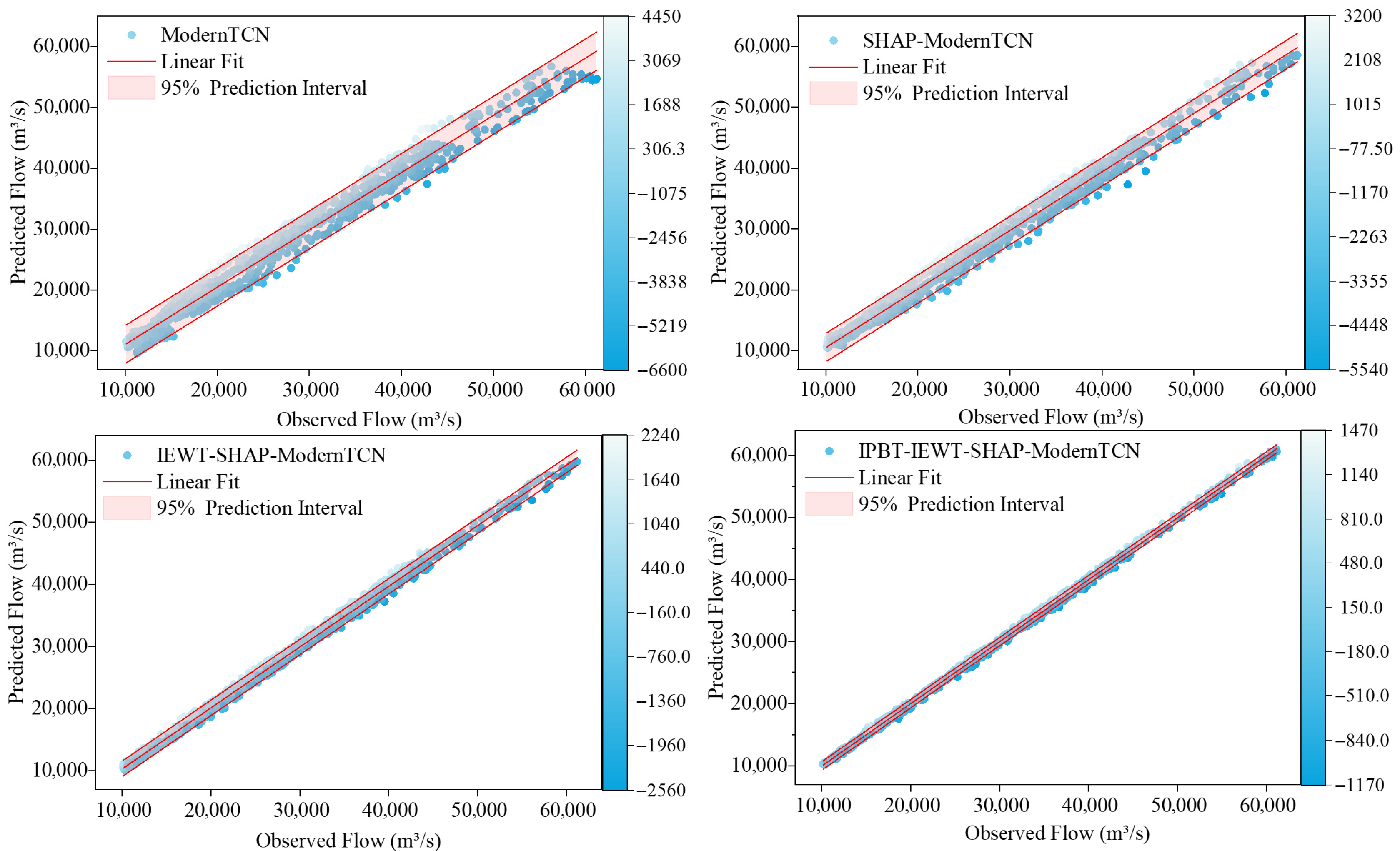
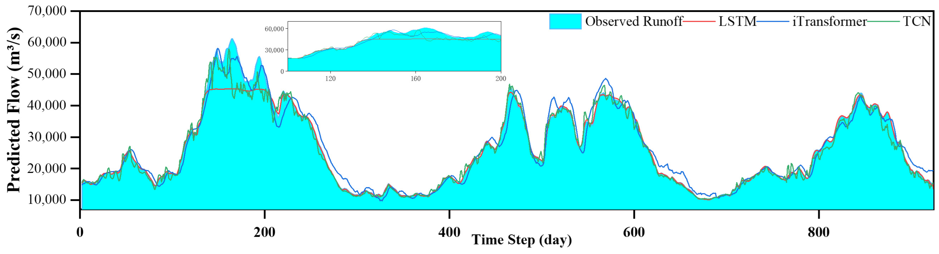
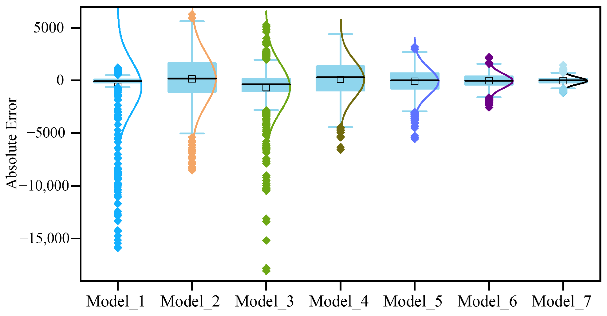
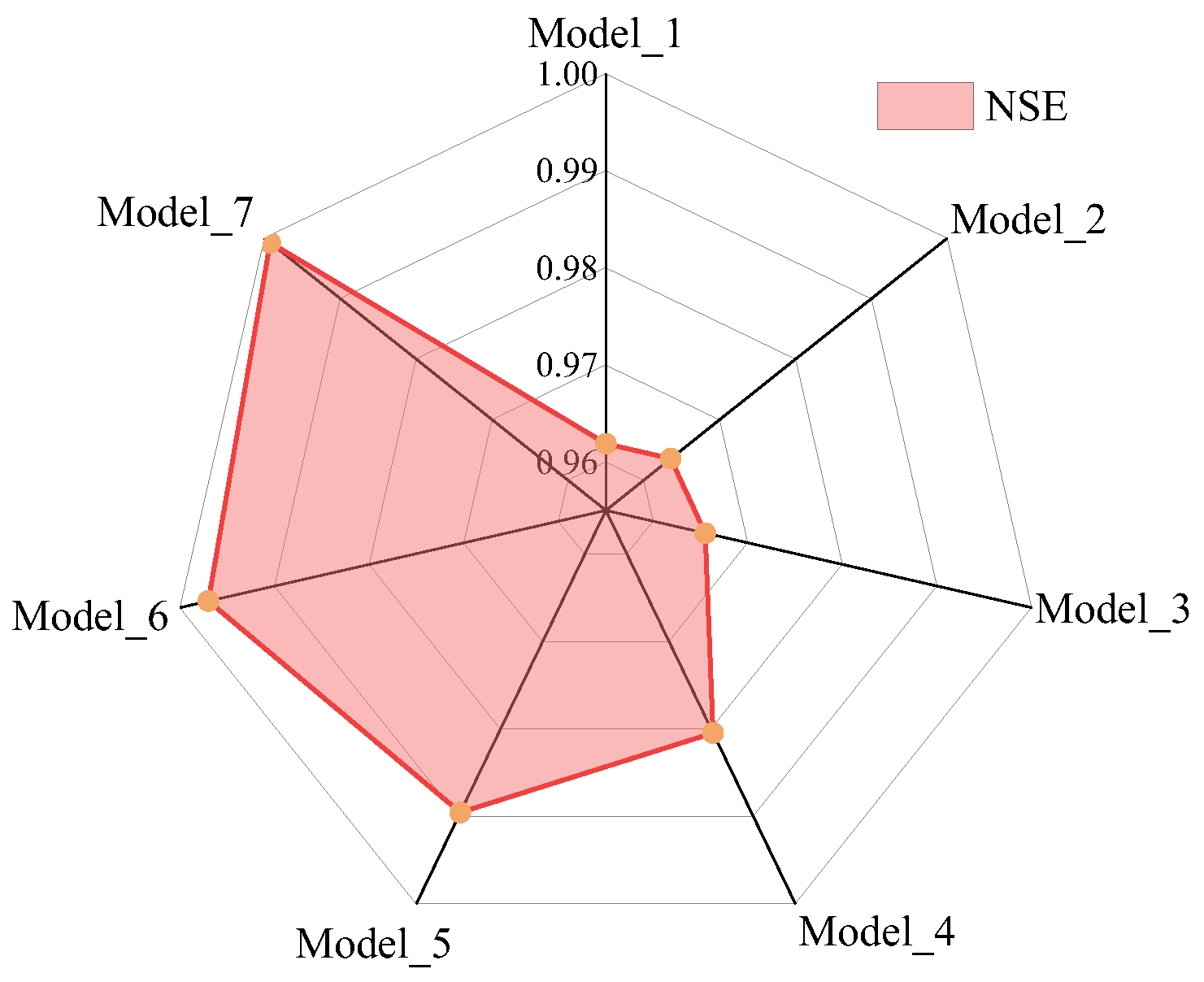
Model Performance Evaluation and Comparison

To verify the effectiveness of the proposed IPBT-IEWT-SHAP-ModernTCN model, several comparative models are established, including: LSTM [32], iTransformer [33], TCN [34], ModernTCN, SHAP-ModernTCN, IEWT-SHAP-ModernTCN. Model performance is comprehensively evaluated in terms of prediction accuracy and stability using multiple statistical indicators, including the Nash–Sutcliffe Efficiency (NSE), Root Mean Square Error (RMSE), Mean Absolute Error (MAE), Symmetric Mean Absolute Percentage Error (sMAPE), Pearson Correlation Coefficient (R), and Coefficient of Determination (R²) [35].

4.2. Data Processing

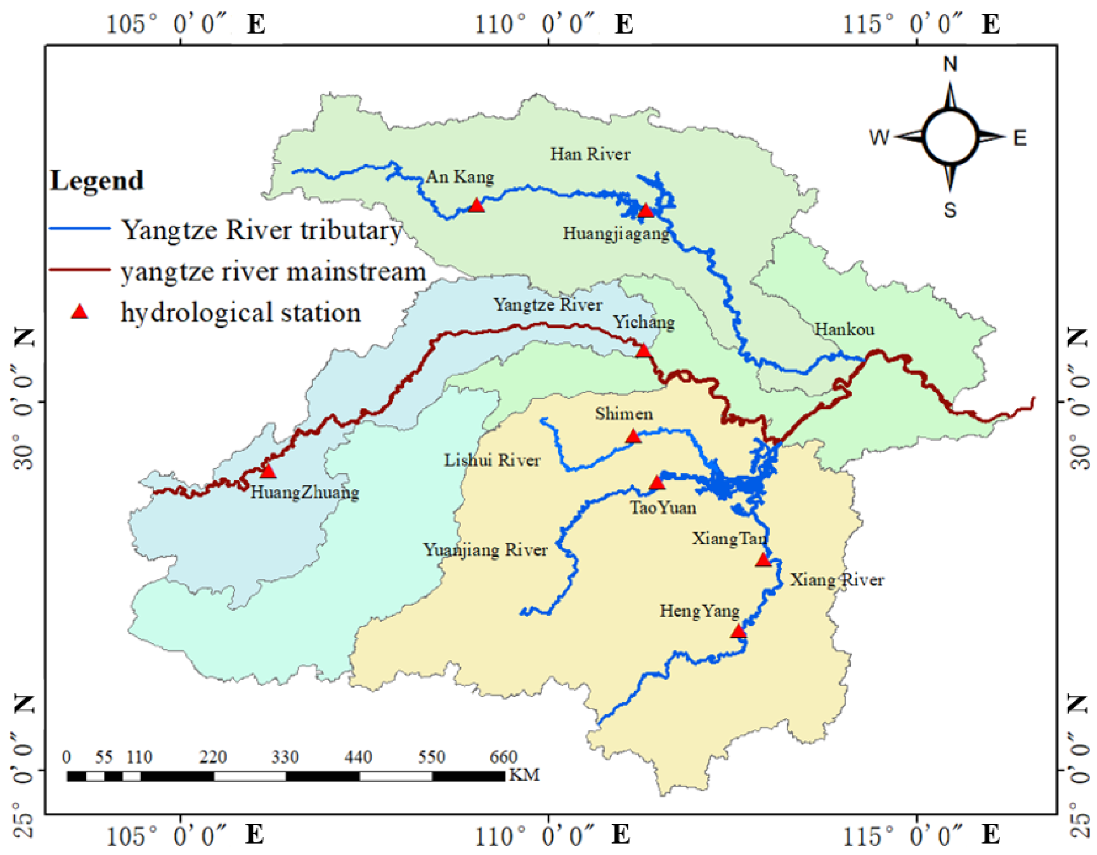
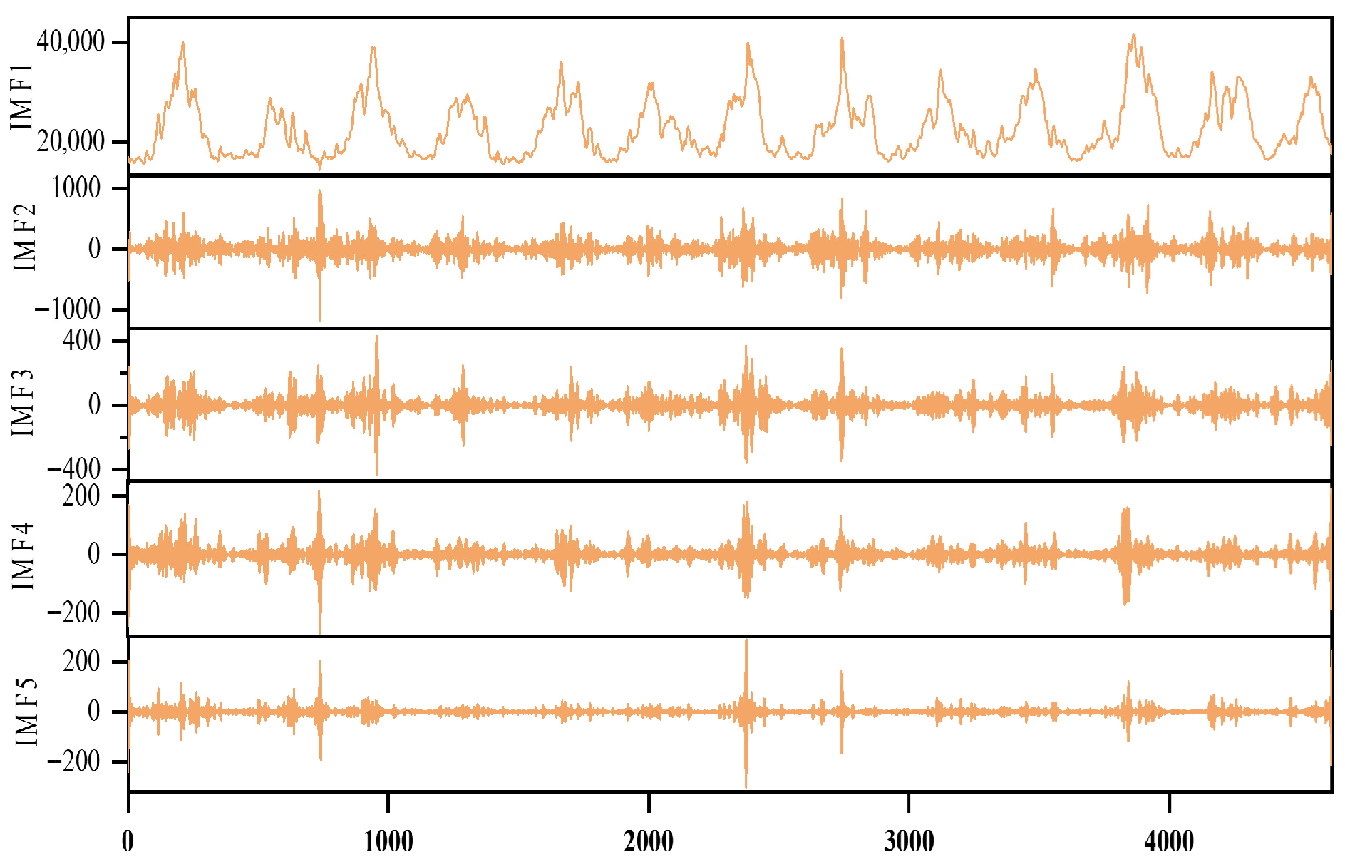
Daily runoff data from 2010 to 2022 were collected from multiple hydrological stations, including Ankang, Huangjiagang, and Huangzhuang along the Hanjiang; Shimen along the Lishui; Hengyang and Xiangtan along the Xiangjiang; Pushi and Taoyuan along the Yuanjiang; as well as the Yichang and Hankou Hydrological Stations. The daily runoff series of the Hankou Station was decomposed using the IEWT method to stabilize the non-stationary signal. The runoff sequence was thus decomposed into five relatively stationary intrinsic mode components, arranged from low to high frequency, as illustrated in Figure 5, this choice is case-dependent and can be adjusted for other datasets depending on the spectral characteristics and the decomposition configuration. The original runoff is decomposed into five intrinsic mode components ordered from low to high frequency. This figure demonstrates how IEWT stabilizes the highly non-stationary daily series into multi-scale components that are later used to enhance prediction under rapid rises and peak-flow fluctuations.

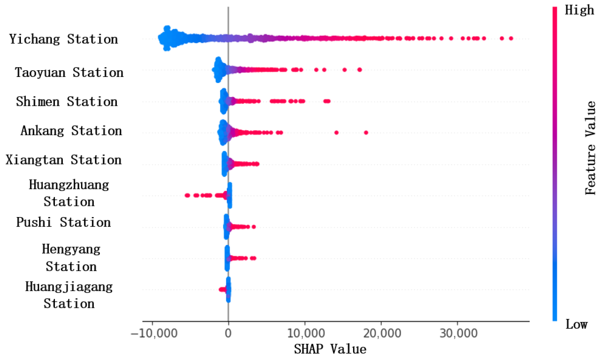
Figure 6 presents the feature importance scatter plot generated using the SHAP (SHapley Additive exPlanations) method, illustrating the contribution of each hydrological station to the model’s prediction. In the figure, the horizontal axis represents the SHAP value, which indicates the magnitude and direction of each station’s influence on the model output—larger absolute SHAP values correspond to stronger contributions, with red points indicating positive influence and blue points representing negative influence. The vertical axis lists the eight key hydrological stations. As shown in the figure, Yichang, Taoyuan, Shimen, Ankang, and Huangzhuang exhibit relatively high SHAP values across the overall distribution, suggesting that these stations play a critical role in the runoff prediction process and serve as important features influencing the model output. Therefore, these stations were selected as the final input features. In contrast, other stations such as Xiangtan and Huangjiagang show more concentrated SHAP value distributions with weaker impacts, and thus were excluded from the model input.

5. Comparisons Results

5.1. Performance Comparison of Daily Runoff Prediction Models

This section evaluates the proposed IPBT-IEWT-SHAP-ModernTCN framework for next-day daily runoff prediction at the Hankou hydrological station. We compare seven models (LSTM, iTransformer, TCN, ModernTCN, SHAP-ModernTCN, IEWT-SHAP-ModernTCN, and IPBT-IEWT-SHAP-ModernTCN) using RMSE, MAE, R, R², sMAPE, and NSE.

Table 1. Runoff Prediction Error Analysis at Hankou Hydrological Station.

Model	RMSE	MAE	R	R2	SMAPE	NSE
LSTM	2446.41	777.1313	0.9844	0.9619	0.0198	0.9619
iTransformer	2392.68	1793.576	0.9819	0.9606	0.0703	0.9636
TCN	2327.41	1257.387	0.9848	0.9655	0.0430	0.9655
ModernTCN	1751.54	1378.486	0.9911	0.9783	0.0580	0.9805
SHAP-ModernTCN	1280.35	958.2164	0.9952	0.9888	0.0384	0.9896
IEWT-SHAP-ModernTCN	687.084	525.5826	0.9987	0.9969	0.0217	0.9969
IPBT-IEWT-SHAP-ModernTCN	342.136	251.0125	0.9996	0.9993	0.0102	0.9992

summarizes the overall quantitative performance and highlights the incremental gains brought by SHAP-based upstream input selection, IEWT-based multi-scale decomposition, and IPBT-based hyperparameter optimization. Figure 7, Figure 8 and Figure 9 provide time-series and scatter-plot comparisons to assess how well each model tracks rising limbs and peak flows. Figure 10 further compares error distributions to evaluate robustness, while Figure 11 and Figure 12 present compact visual summaries of NSE and RMSE across all models.

Figure 7 presents a comparison between the observed runoff and the predicted runoff obtained from the ModernTCN and the proposed IPBT-IEWT-SHAP-ModernTCN models at the Hankou Hydrological Station. The ModernTCN prediction curve (plotted in gray) shows noticeable deviations from the observed runoff (cyan-shaded area), particularly at several peak and trough points, indicating limited capability in accurately capturing runoff fluctuations. In contrast, the IPBT-IEWT-SHAP-ModernTCN prediction curve (plotted in red) provides a finer representation of the runoff dynamics and exhibits a closer alignment with the observed series across peak, valley, and transitional stages. These findings demonstrate that the improved model achieves a marked enhancement in prediction accuracy and stability compared with the baseline ModernTCN.

Figure 8 displays the scatter plots of the predicted versus observed runoff for four models: ModernTCN, SHAP-ModernTCN, IEWT-SHAP-ModernTCN, and IPBT-IEWT-SHAP-ModernTCN. As shown in the figure, the predicted and observed values of all four models exhibit an approximately linear relationship, with the red regression line closely aligned along the diagonal, indicating that the models are capable of capturing the overall variation trend of the observed runoff. Among them, the IPBT-IEWT-SHAP-ModernTCN model presents the lowest dispersion and the tightest clustering around the diagonal line, demonstrating that the successive improvements significantly enhance both the stability and accuracy of runoff prediction. Consequently, the refined composite model achieves predictions that more closely approximate the actual observations, exhibiting superior predictive performance in hydrological runoff forecasting tasks.

Table 1 summarizes the daily runoff prediction performance of the seven models at the Hankou Hydrological Station, as measured by six statistical indicators: Root Mean Square Error (RMSE), Mean Absolute Error (MAE), the Pearson correlation coefficient (R), the coefficient of determination (R²), the symmetric mean absolute percentage error (sMAPE) and the Nash–Sutcliffe efficiency (NSE). Overall, all models achieve NSE values above 0.96, indicating that the competing approaches generally provide reliable daily forecasts at this station. Notably, performance consistently improves along the proposed pipeline, from ModernTCN to SHAP-ModernTCN and then to the IEWT- and IPBT-enhanced variants, as reflected by progressive reductions in RMSE and MAE, and increases in R, R² and NSE.

Figure 9 compares the baseline deep-learning models (LSTM, iTransformer, and TCN) against the observed runoff at Hankou. Consistent with Table 1, TCN provides the best overall accuracy among the three baselines (RMSE = 2327.41; MAE = 1257.39) and tracks the observed series more closely during periods of strong variability and peak-flow fluctuations. It is also noteworthy that iTransformer achieves a slightly lower RMSE than LSTM (2392.68 vs. 2446.41), whereas LSTM yields much lower typical errors (MAE = 777.13 vs. 1793.58; sMAPE = 0.0198 vs. 0.0703). This indicates that LSTM performs more stably under normal-flow conditions but tends to deviate more around high peaks, which is visually evident in Figure 9.

Furthermore, the ModernTCN model introduces structural enhancements based on the traditional TCN, which substantially reduce the RMSE to 1751.54, while both the R² and NSE values show further improvement. These results indicate that ModernTCN possesses a stronger capability in fitting complex runoff fluctuations. However, its MAE is slightly higher than that of the TCN, suggesting that although minor errors increase in some steady-flow intervals, the model demonstrates superior performance in peak-flow prediction.

The SHAP-ModernTCN model, which incorporates SHAP-based feature selection, achieves lower RMSE and MAE values compared with the ModernTCN, indicating that the feature selection process effectively enhances the model’s stability and generalization capability. With the further integration of the Improved Empirical Wavelet Transform (IEWT), the IEWT-SHAP-ModernTCN model exhibits additional improvements across all performance metrics, particularly achieving a reduction in RMSE to 687.08. This significant decrease demonstrates that the combined model attains substantial advances in both peak-flow prediction accuracy and overall error control.

Ultimately, the IPBT-IEWT-SHAP-ModernTCN model, incorporating a Bayesian optimization strategy, achieves the best overall performance across all evaluation metrics.

It attains an RMSE of 342.14 and an MAE of only 251.01, while both the R² and NSE values exceed 0.999, demonstrating that the model not only accurately captures the overall runoff trend but also possesses a remarkable capability to characterize abnormal fluctuations.

These results confirm that the proposed model delivers the most superior and robust predictive performance among all models evaluated in this study.

Table 2. Comparison of Model Abbreviations.

Model_Name	Abbreviation
LSTM	Model_1
iTransformer	Model_2
TCN	Model_3
ModernTCN	Model_4
SHAP-ModernTCN	Model_5
IEWT-SHAP-ModernTCN	Model_6
IPBT-IEWT-SHAP-ModernTCN	Model_7

provides the abbreviations of the seven models, and Figure 10 presents the boxplots of prediction errors, visually depicting the residual distribution characteristics of runoff prediction at the Hankou Hydrological Station. The residuals of traditional models such as LSTM, iTransformer, and TCN exhibit greater dispersion and long-tail distributions, indicating deficiencies in handling extreme or anomalous values. In contrast, the IPBT-IEWT-SHAP-ModernTCN model, which integrates multiple enhancements, demonstrates a more compact residual distribution with a narrower interquartile range and fewer extreme outliers. This concentrated distribution reflects the model’s superior stability and generalization capability across the entire flow range.

Figure 11 and Figure 12 present the RMSE bar chart and NSE radar chart for the seven models, respectively. The radar chart illustrates the NSE performance of different models across multiple evaluation dimensions, while the bar chart quantifies the root mean square error (RMSE) for each model. As shown in the figures, the improved IPBT-IEWT-SHAP-ModernTCN model, which integrates feature selection, signal decomposition, and optimization strategies, achieves the highest NSE values across all evaluation metrics and significantly reduces the RMSE to its lowest level. These results further confirm the model’s superior accuracy and robustness in capturing the complex nonlinear characteristics of hydrological time series.

5.2. Discussion of Robustness and Interpretability in Daily Runoff Prediction Results

The results demonstrate that the proposed IPBT-IEWT-SHAP-ModernTCN framework improves the accuracy, robustness and interpretability of daily runoff forecasting. As summarized in Table 1, the final model achieves the best performance across all metrics (RMSE = 342.14, MAE = 251.01 and NSE ≈ 0.999), indicating a more reliable fit to observed dynamics and reduced uncertainty in operational forecasts.

Interpretability is strengthened through SHAP-based input screening (Figure 6), which provides transparent, station-level attribution and facilitates the removal of redundant upstream inputs. Robustness is also evident in the error distribution comparison (Figure 10), where the proposed model exhibits a more compact residual spread and fewer extreme errors, suggesting enhanced stability under varying hydrological conditions. The decomposition view (Figure 5) also supports this behavior, separating non-stationary runoff into multi-scale components and enabling the ModernTCN to learn smoother low-frequency trends and sharper high-frequency fluctuations more effectively. Overall, Figure 11 and Figure 12 provide a concise visual summary showing that the proposed framework delivers the most stable and efficient forecasting performance consistently outperforming all the other models compared.

6. Conclusions and Future Work

To improve the accuracy and reliability of daily runoff prediction, this study developed an integrated forecasting framework that combines the Improved Empirical Wavelet Transform (IEWT), SHAP-based interpretable feature selection, the Improved Population-Based Training (IPBT) algorithm, and the Modern Temporal Convolutional Network (ModernTCN), namely the IPBT-IEWT-SHAP-ModernTCN model. An empirical case study was conducted using data from the Hankou Hydrological Station, and comparative experiments were performed against benchmark models including LSTM, iTransformer, TCN, and ModernTCN. The main conclusions are summarized as follows:

(1)

Multi-scale decomposition improves the predictability of non-stationary daily runoff. IEWT decomposes the raw runoff series into multi-scale components, which helps mitigate non-stationarity and supports more stable downstream learning, thereby improving overall forecasting reliability.

(2)

Interpretable input selection improves robustness. SHAP-based attribution provides transparent station/feature importance, enabling the removal of redundant inputs and improving robustness, while offering interpretable insights into upstream–downstream influences in the forecasting process.

(3)

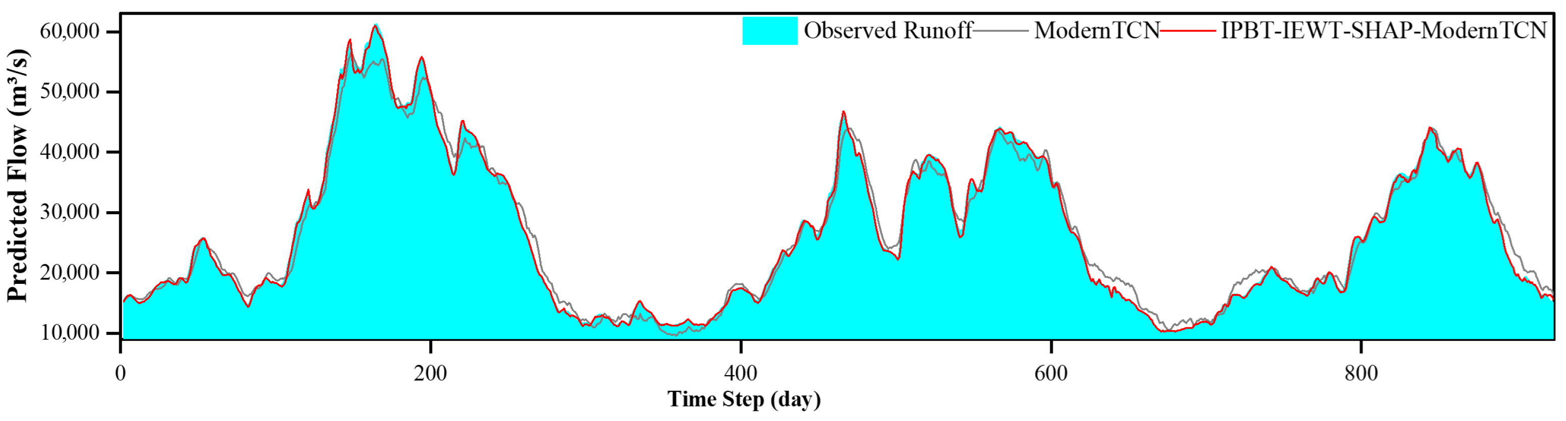
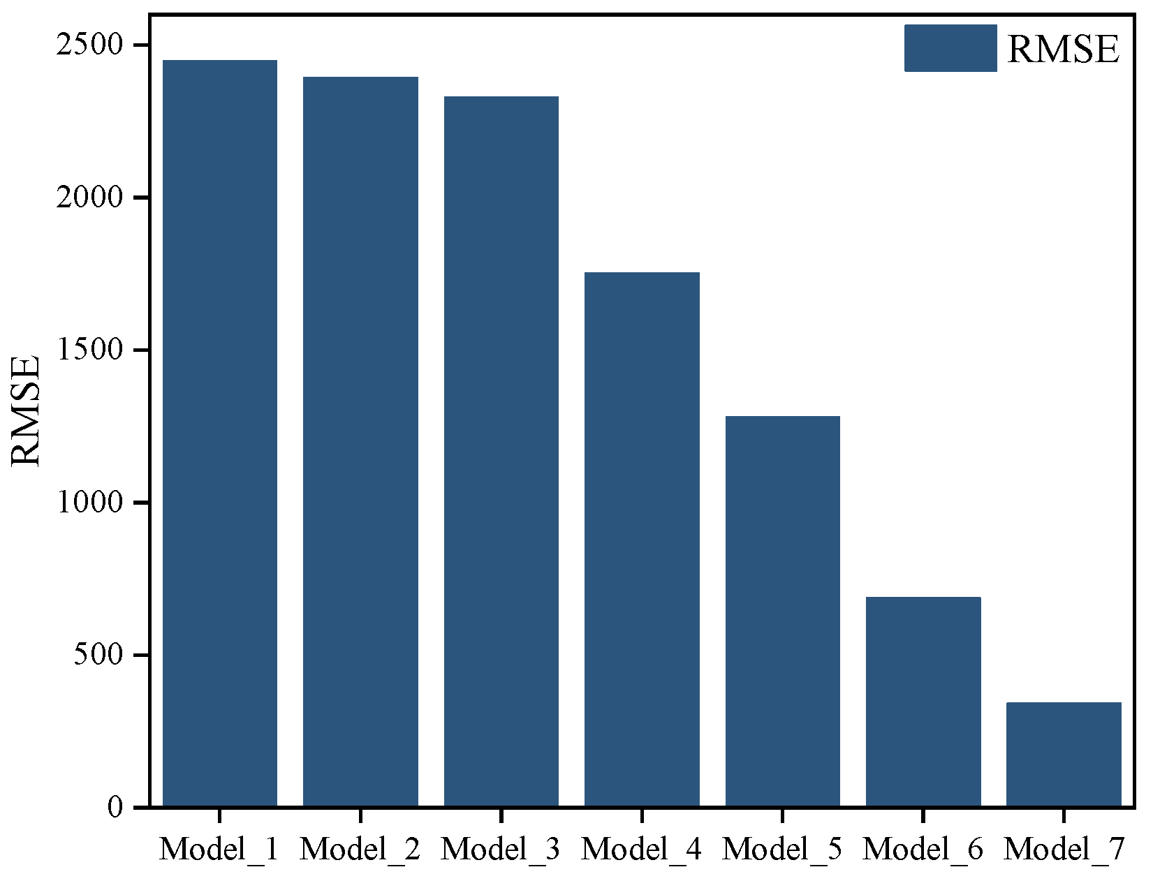
Automated hyperparameter optimization improves model stability and accuracy. IPBT reduces reliance on manual tuning by enabling a dynamic global search within the ModernTCN configuration space. Under the Hankou case study and the experimental settings of this paper, the final model achieved RMSE = 342.14, MAE = 251.01, and NSE = 0.9992, demonstrating strong performance for next-day daily runoff prediction.

(4)

The proposed framework is applicable to next-day runoff forecasting for operational water-resources management at key control stations (e.g., Hankou). By incorporating stable multi-scale decomposition and interpretable input selection, the framework improves forecasting reliability. In the Hankou case study, it reduces RMSE and MAE by approximately 80.47% and 81.79%, respectively, compared with the baseline ModernTCN, indicating more reliable forecasts for this application.

Future work: Future studies will extend the proposed framework to additional basins and hydrological regimes to examine transferability and generalization.

Additionally, we intend to incorporate extra hydro-meteorological and operational drivers (e.g., precipitation, soil moisture and reservoir operation information) when available and further evaluate performance during extreme events and peak-flow conditions.

Finally, we will explore uncertainty quantification and broader benchmarking against alternative decomposition strategies under a unified experimental protocol to strengthen operational applicability.