A DEA-Based Water Distribution Flushing Planning for Prioritizing High-Risk Pipes and Blocks

Abstract

Flushing planning requires utilities to prioritize pipes and service blocks using heterogeneous structural and hydraulic information. This study proposes a data envelopment analysis (DEA)-assisted framework that links pipe-level screening, service-block prioritization, and candidate flushing-segment planning. The framework separately evaluates sedimentation and detachment conditions using input-oriented Banker–Charnes–Cooper (BCC) models based on seven indicators, while avoiding the need to prescribe a common expert-defined weighting vector. The framework was applied to a real water distribution system with 481 pipes and 394 junctions, identifying 88 sedimentation-priority pipes and 12 detachment-priority pipes. Length-weighted aggregation within the existing block structure ranked Blocks 1, 7, 2, and 4 highest, whereas length-normalized analysis identified Block 2 as having the greatest concentration of priority pipes. The leading four-block group remained unchanged across the tested pipe-length exponents, and the top-12 detachment set was retained when the velocity-difference screening level was varied from 0.5 to 2.0 m/s. Additional model-form, preprocessing, indicator-omission, and equal-weight comparisons were used to characterize the sensitivity of pipe-level priorities. Finally, existing valve and hydrant locations were used to delineate five candidate flushing segments in a representative block. The framework provides a systematic basis for directing detailed hydraulic verification and field implementation.

1. Introduction

Water distribution systems are a critical component of urban infrastructure, providing consumers with continuous access to drinking water at stable pressure and quality. During long-term operation, corrosion products, deposits, scale, and other materials can accumulate within pipes and may subsequently be mobilized when hydraulic conditions change, producing discoloration or turbidity at customer taps [1,2]. Source switching, defined in this study as a change in the active supply source or inflow boundary relative to normal operation, can alter both the magnitude and direction of pipe flow. Together with valve operation and other operational disturbances, such hydraulic changes make the proactive identification of pipe sections associated with unfavorable accumulation conditions and material-mobilization potential an important part of water-quality management.

Flushing is among the most widely used maintenance methods for removing loose material from water distribution systems. Conventional flushing, unidirectional flushing (UDF), continuous blow-off, air scouring, and related approaches differ in the degree of hydraulic control and water use. UDF isolates a defined flow path through valve operations and is widely used because it can provide controlled high-velocity cleaning when the network configuration is suitable [2,3]. The location and capacity of available discharge facilities, including hydrants and scour or washout valves, also influence the pipe sections that can be practically isolated and flushed [4]. Detailed UDF design nevertheless requires hydraulic verification of valve states, outlet discharge, achievable flushing velocity, pressure response, and segment length [5,6,7]. Thus, selecting where detailed design should begin is a distinct planning problem that precedes hydraulic confirmation of the final operation.

Beyond avoiding discolored-water events, flushing plans increasingly need to align with sustainability goals under tightening resource constraints, climate variability, and growing urban demand. Reactive responses to incidents often consume large volumes of potable water, disrupt service, and erode public trust. Utilities therefore require proactive, transparent, and reproducible prioritization tools that can focus efforts where it matters most, thereby reducing non-revenue water, curbing unnecessary operational emissions, and minimizing social impacts from unplanned water outages.

Flushing plans are typically implemented on a block or segment basis, because simultaneous flushing of the entire network is practically unfeasible. Establishing flushing priorities by determining “block risk” based on the potential for water quality incidents and hydraulic conditions at the block level is essential. Prior studies aimed at identifying high-risk pipes or blocks have primarily employed multi-criteria decision analysis (MCDA) techniques with representative methods, including analytic hierarchy process (AHP), technique for order preference by similarity to ideal solution (TOPSIS), and preference ranking organization method for enrichment evaluation (PROMETHEE) [8,9,10,11]. The evaluation criteria incorporated several physical and operational factors such as velocity, incident history, diameter, installation year, and pressure, which were integrated via weighted assessments. Alaggio et al. [12] applied complex network theory, using centrality indicators and path stability to identify key high-risk pipes. By contrast, Salehi et al. [13] conducted detailed risk analyses that reflected 19 factors, including velocity, stagnation time, and water quality indices, using fuzzy-logic-based MCDA. These studies incorporated the mechanical characteristics of the pipes, hydraulic conditions, social impacts, and environmental factors. Such approaches are particularly useful when an explicit preference structure can be established for the decision problem. However, when criterion weights are determined by users or experts, the relative importance assigned to individual factors may vary among utilities and decision makers. Consequently, the resulting priority ranking reflects not only the observed network conditions but also the weighting structure adopted for the assessment.

As an alternative, nonparametric efficiency analysis methods such as data envelopment analysis (DEA) have been applied in the water distribution field. DEA measures the relative efficiency of multiple decision-making units (DMUs) using multiple input and output indicators within a linear-programming framework. Rather than prescribing a common set of indicator weights in advance, DEA determines admissible weights endogenously for each DMU under the same model constraints [14]. This feature is useful for screening problems in which the relative importance assigned to heterogeneous structural and hydraulic indicators may vary among users or utilities. The resulting weights nevertheless depend on the adopted DEA model and the analyzed dataset and do not describe the physical importance of the individual indicators.

The scope of DEA applications in water supply systems has been expanding. Kamarudin et al. [15] applied network DEA to Malaysian water supply operators, integrating undesirable outputs such as non-revenue water and leakage volumes to diagnose operator and process inefficiencies and to propose operational improvement directions. Gidion et al. [16] used network DEA to evaluate process-level efficiencies of urban water utilities, deriving detailed performance enhancement strategies and benchmarking both overall and individual process efficiencies. More recently, DEA has been increasingly employed for vulnerability analyses of distribution networks at the block or zone level. Palomero-González et al. [17] evaluated block-level operational data from Valencia, Spain, using a DEA-based Russell directional distance model to identify vulnerability zones based on maintenance costs, leakage, and water quality. Yin et al. [18] applied a dynamic network DEA to 246 Chinese urban water operators, providing in-depth analyses of efficiencies across production and supply processes as well as regional disparities.

Previous DEA applications have addressed utility performance, leakage, operational efficiency, resilience, and vulnerability. The remaining issue for flushing planning is not whether DEA can be applied to water systems, but how pipe-level multi-indicator screening can be translated into the operational units used for maintenance. In particular, pipe and block priorities do not by themselves specify how a utility should identify candidate flushing segments from its existing service-block boundaries, valves, hydrants, and network connectivity.

Previous work has demonstrated the applicability of DEA to pipe-level screening and service-block prioritization using sedimentation- and detachment-related conditions [19]. The present study extends this decision process to flushing planning by linking the resulting pipe and block priorities with the existing valve and hydrant configuration to identify candidate flushing segments. This provides a continuous planning sequence from network-wide screening to the selection of candidate locations for detailed hydraulic evaluation. The framework is applied to actual network data from City A. The objectives are to identify relative priority pipes without prescribing one common expert-defined indicator-weight vector, aggregate the resulting classes within existing service blocks, examine the stability of the resulting priorities under alternative analytical and aggregation conditions, and translate a selected priority block into candidate flushing segments using explicit facility and connectivity rules. The study is framed as a utility-scale planning case study; flushing velocity, pressure response, discharge, water volume, and field water-quality response remain subsequent engineering and validation tasks.

2. Materials and Methods

This study presents a DEA-assisted framework that evaluates relative pipe priority, aggregates the resulting classes within existing service blocks, and uses the installed valve–hydrant configuration to define candidate flushing segments. Here, the term “high-risk” denotes a relative planning category within the analyzed network rather than an absolute probability of a water-quality incident.

All data used in the analysis were derived from the actual network database and hydraulic simulation results. The methodological procedure was organized sequentially to describe the rationale for selecting the influencing factors, the calculation of each indicator, the theoretical background and application of DEA, and the subsequent processes—including identifying high-risk pipes, defining block priorities, and formulating candidate UDF plans.

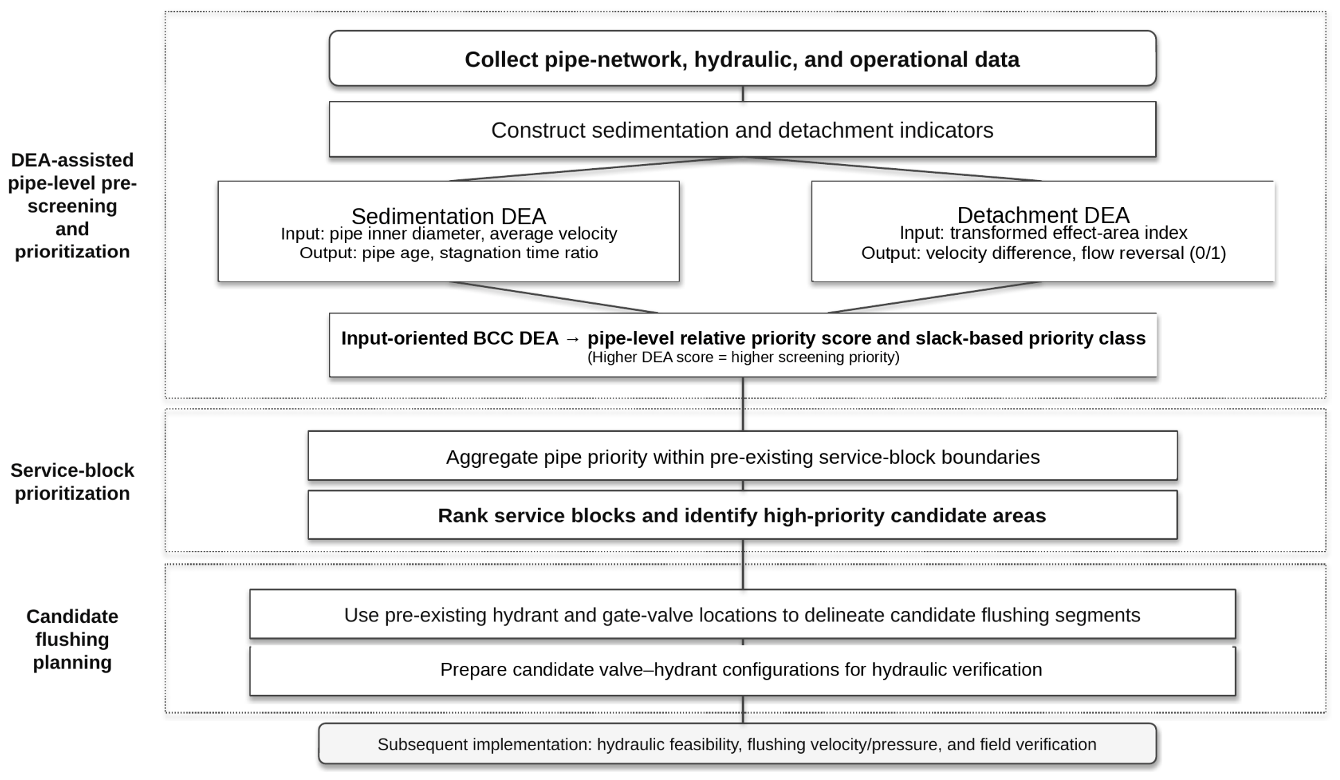
The overall procedure is organized into four stages. First, hydraulic and facility data are used to construct sedimentation and detachment indicators. Second, separate input-oriented BCC DEA models and slack information are used to classify relative pipe priority. Third, the pipe classes are aggregated within the utility’s pre-existing service blocks using class coefficients and pipe length. Fourth, candidate flushing segments are delineated from the installed gate-valve and hydrant configuration and are then passed to subsequent hydraulic verification. Thus, the proposed procedure distinguishes network-wide prioritization and candidate UDF planning from the final hydraulic design required before field implementation.

2.1. Selection of Influencing Factors for Identifying High-Risk Pipes

In this study, high-risk pipes are defined operationally as pipes that exhibit relatively unfavorable combinations of conditions associated with sediment accumulation under normal operation or material detachment under the examined source-switching disturbance. The term therefore denotes a relative planning category within the analyzed network. Sedimentation indicators describe structural and hydraulic conditions associated with deposition, whereas detachment indicators describe hydraulic disturbance together with the potential extent of impact.

2.1.1. Preliminary Investigation for Determining Influencing Factors

The planning of maintenance activities in water distribution systems, particularly proactive interventions such as flushing or pipe replacement, has evolved to incorporate comprehensive assessments of various influencing factors. Existing studies have categorized these factors into structural, hydraulic, operational, and environmental elements and incorporated them into diverse models that combine quantitative data analyses with expert judgment.

For example, Tscheikner-Gratl et al. [20] applied four MCDA techniques (AHP, TOPSIS, PROMETHEE, and ELECTRE) in an Austrian case study and demonstrated that prioritization for pipeline rehabilitation varied significantly by method. Their study used indicators such as failure probabilities, service interruption impacts, maintenance costs, pressure adequacy, and hydraulic resilience, and conducted sensitivity analyses to examine each variable’s contribution. Carriço et al. [11] assessed a transmission network in a Portuguese industrial district using multicriteria evaluations with ELECTRE III and weighted sum models based on nine indicators: hydraulic capacity, storage capability, asset value, leakage rate, structural grade, service interruption risks, burst probabilities, and maintenance costs. Input variables were calculated using both measured and simulated data, illustrating a quantitative analysis that incorporated operational performance and hydraulic risks.

Raspati et al. [21] applied a random forest approach in Trondheim, Norway, to predict pipe failure probabilities and quantify service disruptions through reliability analyses, employing pipe age, material, diameter, length, and historical failure records as inputs. Composite risk scores were calculated by multiplying failure probabilities by service loss quantities, integrating structural risks and hydraulic importance. Drici et al. [22] applied AHP in Khemis Miliana, Algeria, performing a hierarchical analysis that incorporated diameter, age, pressure-deficient zones, leak frequencies, and seismic risks by combining expert surveys with hydraulic simulations to select pipes for replacement.

Recent studies have increasingly combined artificial intelligence with hybrid approaches. Elshaboury and Marzouk [23] proposed an integrated framework in Giza, Egypt, combining artificial neural network-based pipe condition index predictions, multi-objective optimization, and multi-criteria assessments using variables such as diameter, length, installation year, thickness, and burial depth. Xing et al. [24] used Bayesian networks in a Hong Kong water distribution system to predict pipe burst probabilities and quantitatively evaluate variable importance and interactions.

Regarding flushing strategies, Husband and Boxall [25] reported that UK water utilities typically adopt a reactive approach in selecting flushing sections, primarily in response to complaints about turbid water. However, some utilities have preselected proactive flushing zones using quantitative indicators such as complaint frequency, velocity, turbidity, and residual disinfectant concentration, highlighting the need to incorporate quantitative criteria into flushing plans. Speight et al. [26] used machine learning to analyze water quality indicators (iron, manganese, chlorine, aluminum, and nitrate), pipe aging, failure probabilities, and operational data to identify key causes of turbidity.

Vairavamoorthy et al. [27] developed a pipe-condition assessment model integrating various factors such as pipe specifications, age, installation conditions, soil corrosion, and failure probabilities. Their model incorporated internal and external pipe coatings, installation year, and groundwater levels to predict pipe conditions. Islam et al. [28] evaluated external factors, pressure, and pipe aging to predict leaks, whereas Kwon [29] proposed a model that determined improvement priorities in water networks by combining failure probabilities with pipe aging. Kim et al. [30] introduced a score equalization model for assessing pipe aging using data such as environmental conditions, diameter, installation year, and leakage or burst histories. Yoo [31] developed a practical priority assessment model integrating failure probabilities with relative importance.

These studies indicate that structural factors (pipe age, material, diameter, and failure history), hydraulic factors (velocity, pressure deficiencies, and unstable flows), operational factors (leak frequencies, maintenance costs, and service-disruption histories), and environmental and water quality factors (turbidity complaints, disinfectant concentrations, and soil corrosivity) have been widely used for priority assessments. Nevertheless, interviews with field experts revealed that operational, environmental, and water quality data are often lacking in domestic and international practice. Therefore, this study constructed an evaluation model focusing on structural and hydraulic factors while flexibly defining influencing factors to enable extended application in areas with sufficient data.

2.1.2. Sedimentation Factors

Sediment accumulation within water distribution pipes is an important contributor to water quality deterioration and can result from interacting physical, chemical, and hydraulic conditions. In sections with low velocities or prolonged stagnation, conditions may favor the accumulation of scale, slime, and other loose materials on the inner pipe surfaces, which can subsequently contribute to water quality incidents when hydraulic conditions change. This study aimed to quantify the relative potential for sediment accumulation by selecting core influencing factors that could be evaluated consistently across the study network.

The sedimentation indicators were selected by considering literature support, practical interpretation, redundancy among candidate variables, and data availability. Four indicators were retained: pipe age, pipe inner diameter, average velocity, and stagnation time ratio. Their DEA input/output roles are defined in

Table 1. Properties and definitions of sediment and detachment factors.

Factor	Criteria	Description	Priority Direction	Unit	DEA Role
Sedimentation	Pipe age	Base year–Year of installation	Higher	Year	Output
	Pipe inner diameter	Internal diameter of pipe	Lower	mm	Input
	Average velocity	24-h mean velocity magnitude under normal operation	Lower	m/s	Input
	Stagnation time ratio	Number of hourly zero-velocity steps/24	Higher	-	Output
Detachment	Effect area	Flow-based hydraulic influence proxy; transformed value used as DEA input	Higher raw value	-	Input
	Velocity difference	Maximum hourly absolute velocity difference between normal and source-switching conditions; values < 0.5 m/s assigned zero	Higher	m/s	Output
	Flow reversal	1 if any flow-direction reversal occurs under source switching; otherwise 0	Occurrence	-	Output

; no single indicator is treated as an independent predictor of sediment accumulation.

Pipe age refers to the number of years since installation and is retained as a structural indicator because longer service time can be associated with deterioration, corrosion products, and deposit accumulation [26,27,29]. In this study, pipe age was calculated from installation-year information in the GIS database. Pipe age is not assumed to determine hydraulic velocity, which is governed by network topology, demand, pipe size, supply path, and operation.

Pipe inner diameter was obtained from the facility database and retained as a structural descriptor. In the sedimentation DEA model, smaller diameter values are oriented toward the priority frontier, but diameter is evaluated jointly with velocity, stagnation, and age rather than interpreted as a stand-alone causal measure of sediment accumulation. Accordingly, its role in the model is to provide structural information that complements the hydraulic and temporal indicators rather than to imply that smaller pipes necessarily contain more deposited material.

Average velocity represents the 24-h mean pipe-velocity magnitude under normal operation. Persistently low-flow conditions are associated with deposition and discoloration concerns [2,6], so average velocity is used as a hydraulic screening indicator together with the remaining structural and temporal variables.

Stagnation time ratio represents the proportion of the 24 hourly reporting steps at which pipe velocity is zero. It therefore describes intermittent no-flow periods that can be obscured by a daily mean velocity. The ratio was calculated as the number of zero-velocity reporting steps divided by 24.

The four sedimentation indicators were used jointly in the DEA model. Pipe inner diameter and average velocity were assigned as DEA inputs because lower values are oriented toward higher screening priority, whereas pipe age and stagnation time ratio were assigned as DEA outputs because higher values are oriented toward higher priority. The input/output designation reflects the mathematical orientation adopted in the DEA model and does not imply a direct physical cause-and-effect relationship. Table 1 summarizes these definitions and roles.

2.1.3. Detachment Factors

Sediments and scales that accumulate under normal operation can be mobilized when an operational disturbance changes the magnitude or direction of flow. The detachment analysis therefore compares the normal hydraulic condition with a defined emergency source-switching condition and considers the potential influence range of an affected pipe [2,6].

Three complementary detachment indicators were used: effect area, velocity difference, and flow reversal. Their operational definitions follow the established pipe-screening procedure [19], but they represent different aspects of the same planning problem: potential influence range, magnitude of hydraulic change, and occurrence of a directional reversal.

Velocity difference was calculated by comparing the normal-operation and source-switching simulations at corresponding hourly reporting steps. For each pipe, the absolute velocity difference was calculated at each step, and the maximum value over the 24-h simulation was retained. Values below 0.5 m/s were assigned zero, whereas values equal to or greater than 0.5 m/s retained their continuous magnitude. The 0.5 m/s value is used as an operational screening rule in the adopted procedure rather than as a universal physical threshold for sediment detachment. Accordingly, velocity difference represents the magnitude of the hydraulic disturbance that may contribute to material mobilization when deposited material is present; the conditions associated with sediment accumulation itself are evaluated separately in the sedimentation model.

Flow reversal was represented as a binary indicator. A value of 1 was assigned when the sign of pipe flow differed between the normal-operation and source-switching conditions at one or more reporting steps, and 0 otherwise. Thus, the variable records whether a reversal occurs under the examined disturbance rather than the number or frequency of reversals within a day.

Effect area is used as a flow-based proxy for the potential influence associated with an affected pipe. For pipe $i$, the raw effect-area indicator was calculated as

$$E_i={\displaystyle \frac{Q_i}{{\displaystyle {\sum }_{j=1}^n}{Q}_j}}$$

(1)

where $Q_i$ denotes the representative pipe-flow value used for pipe $i$, and the denominator represents the sum of the corresponding flow values for the $n$ pipes included in the analysis. Thus, $E_i$ expresses the relative contribution of a pipe to the total reference flow used in the analysis. It is a flow-based influence proxy rather than a geometric GIS area, a direct customer count, or a delineated downstream service area. A larger $E_i$ indicates a greater relative hydraulic influence. To make its direction consistent with the input-oriented DEA formulation, the transformed value

$$g_i=\ln \left({\displaystyle \frac{1}{E_i}}\right)$$

(2)

was used as the DEA input after normalization, so that a pipe with a larger raw effect-area value is represented by a smaller input value and is therefore oriented toward higher detachment priority.

2.2. DEA Model

Flushing cannot be performed simultaneously across all sections of a water distribution system. Therefore, similar to other maintenance strategies for water networks, establishing priorities before implementation is essential. This study uses the concept of high-risk pipes to determine flushing priorities. As defined in Section 2.1, high-risk pipes represent pipes with relatively unfavorable combinations of sedimentation- or detachment-related conditions within the analyzed network, and DEA was employed to identify their relative screening priorities.

DEA is a non-parametric, linear programming-based analytical technique used to quantitatively assess the relative efficiency of multiple DMUs using various DEA-input and DEA-output variables under a common analytical objective. This is particularly advantageous when multiple variables with different characteristics are considered simultaneously because DEA does not require a common set of input and output weights to be prescribed in advance. Instead, admissible weights are determined endogenously for each evaluated DMU under the same model constraints [14]. Moreover, DEA can simultaneously handle variables with different physical units, such as pipe diameter in millimeters and velocity in meters per second, facilitating relative comparisons among DMUs. The analysis also provides slack values, which indicate the remaining input excesses or output shortfalls after radial adjustment. Its capacity to incorporate multiple criteria concurrently makes DEA particularly suitable for screening complex urban water systems.

In DEA, the relative efficiency of each DMU is generally expressed as the ratio of the weighted DEA-output variables to the weighted DEA-input variables. A DMU with an efficiency score equal to 1 lies on the efficient frontier, whereas a DMU with a score below 1 lies inside the frontier. In the present study, however, the DEA variables are intentionally oriented toward sedimentation or detachment priority; consequently, a score closer to 1 is interpreted as a higher relative screening priority rather than as superior operational performance. The general weighted-ratio form is given by Equation (3).

$${\mathrm{E}\mathrm{f}\mathrm{f}\mathrm{i}\mathrm{c}\mathrm{i}\mathrm{e}\mathrm{n}\mathrm{c}\mathrm{y}}_k={\displaystyle \frac{{\displaystyle {\sum }_{r=1}^s}{u}_r{y}_{rk}}{{\displaystyle {\sum }_{i=1}^m}{v}_i{x}_{ik}}}$$

(3)

where $m$ and $s$ denote the numbers of DEA-input and DEA-output variables, respectively; $x_{ik}$ and $y_{rk}$ denote input $i$ and output $r$ for the evaluated pipe $k$; and $v_i$ and $u_r$ are the non-negative weights assigned to the corresponding inputs and outputs. For the sedimentation model, pipe diameter and average velocity are used as inputs, while pipe age and stagnation time ratio are used as outputs. For the detachment model, the transformed effect-area variable defined in Equation (2) is used as the input, while velocity difference and flow reversal are used as outputs. The weights in Equation (3) are optimization variables determined separately for each DMU and should not be interpreted as fixed physical importance coefficients.

Among the models most commonly employed in DEA analyses are the Charnes–Cooper–Rhodes (CCR) model, which assumes constant returns to scale (CRS) [32], and the Banker–Charnes–Cooper (BCC) model, which assumes variable returns to scale (VRS) [33]. Each model can be further classified as input-oriented (I) or output-oriented (O), depending on whether the radial adjustment is made primarily through the inputs or outputs.

The CCR model, introduced by Charnes et al. [32], assumes CRS, so the reference frontier is constructed without accounting for scale-dependent changes in efficiency. This model considers $n$ DMUs, each using $m$ DEA-input variables $x_{ij}\left(i^{,}{=}^{,}1\dots m\right)$ to produce $s$ DEA-output variables $y_{rj}\left(r^{,}{=}^{,}1\dots s\right)$. The fractional weighted-ratio formulation can be converted into a linear programming problem by normalizing the weighted input. For implementation and slack analysis, the corresponding envelopment formulations were used. The input- and output-oriented CCR models are expressed in Equations (4) and (5), respectively.

$$\begin{array}{ll}\min Z_k^I& ={\theta }_k-\epsilon \left({\displaystyle \sum _{i=1}^m}{s}_i^{-}+{\displaystyle \sum _{r=1}^s}{s}_r^{+}\right)\\ \hfill \mathrm{s}.\mathrm{t}.& {\displaystyle \sum _{j=1}^n}{x}_{ij}{\lambda }_j+s_i^{-}={\theta }_k{x}_{ik}, i=1,\dots ,m,\\ & {\displaystyle \sum _{j=1}^n}{y}_{rj}{\lambda }_j-s_r^{+}=y_{rk}, r=1,\dots ,s,\\ & {\lambda }_j, s_i^{-}, s_r^{+}\ge 0.\end{array}$$

(4)

$$\begin{array}{ll}\max Z_k^O& ={\psi }_k+\epsilon \left({\displaystyle \sum _{i=1}^m}{s}_i^{-}+{\displaystyle \sum _{r=1}^s}{s}_r^{+}\right)\\ \hfill \mathrm{s}.\mathrm{t}.& {\displaystyle \sum _{j=1}^n}{x}_{ij}{\lambda }_j+s_i^{-}=x_{ik}, i=1,\dots ,m,\\ & {\displaystyle \sum _{j=1}^n}{y}_{rj}{\lambda }_j-s_r^{+}={\psi }_k{y}_{rk}, r=1,\dots ,s,\\ & {\lambda }_j, s_i^{-}, s_r^{+}\ge 0.\end{array}$$

(5)

Here, $k$ denotes the evaluated DMU, $j$ indexes the reference DMUs, ${\lambda }_j$ is the peer-combination weight, ${\theta }_k$ is the radial contraction factor in the input-oriented model, and ${\psi }_k$ is the radial expansion factor in the output-oriented model. The variables $s_i^{-}$ and $s_r^{+}$ denote input and output slacks, respectively, and $\epsilon$ is a small non-Archimedean constant used to prioritize slack adjustment after the radial component.

The CCR model does not account for differences in returns to scale. Banker et al. [33] proposed the BCC model by introducing the convexity constraint

$${\displaystyle \sum _{j=1}^n}{\lambda }_j=1,$$

(6)

which allows the reference frontier to represent variable returns to scale. The input- and output-oriented BCC formulations are therefore expressed in Equations (7) and (8), respectively.

$$\begin{array}{ll}\min Z_k^I& ={\theta }_k-\epsilon \left({\displaystyle \sum _{i=1}^m}{s}_i^{-}+{\displaystyle \sum _{r=1}^s}{s}_r^{+}\right)\\ \hfill \mathrm{s}.\mathrm{t}.& {\displaystyle \sum _{j=1}^n}{x}_{ij}{\lambda }_j+s_i^{-}={\theta }_k{x}_{ik}, i=1,\dots ,m,\\ & {\displaystyle \sum _{j=1}^n}{y}_{rj}{\lambda }_j-s_r^{+}=y_{rk}, r=1,\dots ,s,\\ & {\displaystyle \sum _{j=1}^n}{\lambda }_j=1,\\ & {\lambda }_j, s_i^{-}, s_r^{+}\ge 0.\end{array}$$

(7)

$$\begin{array}{ll}\max Z_k^O& ={\psi }_k+\epsilon \left({\displaystyle \sum _{i=1}^m}{s}_i^{-}+{\displaystyle \sum _{r=1}^s}{s}_r^{+}\right)\\ \hfill \mathrm{s}.\mathrm{t}.& {\displaystyle \sum _{j=1}^n}{x}_{ij}{\lambda }_j+s_i^{-}=x_{ik}, i=1,\dots ,m,\\ & {\displaystyle \sum _{j=1}^n}{y}_{rj}{\lambda }_j-s_r^{+}={\psi }_k{y}_{rk}, r=1,\dots ,s,\\ & {\displaystyle \sum _{j=1}^n}{\lambda }_j=1,\\ & {\lambda }_j, s_i^{-}, s_r^{+}\ge 0.\end{array}$$

(8)

Because no constant proportional relationship between the selected risk-oriented inputs and outputs was assumed across pipes with heterogeneous structural and hydraulic characteristics, the input-oriented BCC model in Equation (7) was adopted for the sedimentation and detachment analyses. The resulting radial score and slack information were then used for the pipe classification described in Section 2.3.

2.3. Identification of High-Risk Pipes Using DEA

As previously discussed, this study employed DEA to quantitatively assess the relative priority of pipes based on sedimentation- and detachment-related conditions within a water distribution network, thereby identifying high-risk pipes for flushing planning. The four sedimentation factors and three detachment factors selected for pipe risk assessment have different measurement units and characteristics, making it inherently challenging to integrate their relationships within a common screening framework. In conventional multi-criteria assessments, such diverse factors generally require predefined weights to reflect their relative importance, which can introduce dependence on the weighting assumptions adopted for the analysis. DEA, as a non-parametric efficiency analysis technique, instead determines admissible weights endogenously under common model constraints, making it suitable for evaluating heterogeneous pipe conditions without prescribing a single common weighting vector. This weighting structure also allows different combinations of indicators to contribute to high relative priority among individual pipes rather than requiring all high-priority pipes to exhibit the same indicator pattern.

To identify high-risk pipes, DEA models were structured to independently evaluate sedimentation- and detachment-related conditions, thereby performing parallel analyses of the two mechanisms. The sedimentation analysis targeted pipes exhibiting relatively unfavorable combinations of structural and hydraulic conditions associated with internal deposition under normal operation. Since scale and sediment accumulation can reduce the effective cross-sectional area of a pipe, increase head loss, and contribute to water-quality deterioration when accumulated material is subsequently mobilized, such pipes warrant proactive management and maintenance. Consequently, sedimentation-priority pipes were considered candidate locations for preferential inspection and cleaning within the subsequent flushing-planning procedure.

In this study, the DEA formulation was intentionally designed so that pipes with less favorable sedimentation- or detachment-related conditions appear more efficient in the DEA sense, allowing these pipes to be interpreted as higher-priority flushing targets. Variables that indicate higher priority when smaller, such as pipe diameter and average velocity, were treated as DEA-input variables, whereas variables that indicate higher priority when larger, such as pipe age and stagnation time ratio, were treated as DEA-output variables. This mapping enables the DEA efficiency score to function as a relative screening index rather than as a measure of conventional operational efficiency. Accordingly, higher DEA scores identify pipes located on or closer to the adopted priority frontier and are interpreted as requiring greater attention in subsequent flushing planning.

For the sedimentation DEA model, pipe diameter and average velocity were selected as DEA-input variables, while pipe age and stagnation time ratio were treated as DEA-output variables. Pipe age and stagnation time ratio were used as DEA-output variables because higher values are oriented toward greater sedimentation priority, whereas smaller pipe diameters and lower velocities are oriented toward greater priority and were therefore designated as DEA-input variables. Pipe age was calculated from the installation year, and pipe diameter was obtained from the facility database. The hydraulic characteristics of each pipe, namely average velocity and stagnation time ratio, were derived from the 24-h extended-period simulation (EPS) under normal operating conditions using hourly demand patterns. Specifically, stagnation time ratio was defined as the proportion of hourly reporting steps during which pipe velocity was equal to 0 m/s. For example, if velocity remained at 0 m/s for 6 of the 24 hourly reporting steps, the stagnation time ratio was calculated as 6/24 = 0.25.

For the detachment analysis, pipes were evaluated by comparing normal and source-switching hydraulic conditions together with the potential influence associated with an affected pipe. Effect area represents the flow-based hydraulic influence defined in Section 2.1.3, velocity difference represents the maximum hourly magnitude of hydraulic change between the two operating conditions, and flow reversal records whether the direction of flow changes under source switching. The transformed effect-area variable, $g_i$, defined in Equation (2), was used as the DEA input, whereas velocity difference and flow reversal were used as DEA outputs. The resulting DEA score is interpreted as a relative detachment-screening priority under the examined source-switching scenario rather than as a direct probability of sediment release.

The DEA models were therefore designed such that pipes with higher relative priorities in terms of sedimentation or detachment are evaluated as more “efficient” in the DEA sense compared with the other pipes in the analyzed network. The objective is not to assign an absolute risk probability to each pipe, but to identify a subset of pipes that warrants greater attention through relative comparison among the DMUs.

Because no constant proportional relationship between the risk-oriented DEA inputs and outputs was assumed across pipes with heterogeneous structural and hydraulic characteristics, the input-oriented BCC model in Equation (7) was applied to both the sedimentation and detachment analyses. A DEA score of 1 identifies a pipe on the adopted frontier, and slack information was used to further distinguish pipes sharing the same radial score. For the sedimentation model, frontier pipes were divided into the 1++, 1+, and 1− planning classes according to their slack status, following the adopted classification procedure [19]. Non-frontier pipes were assigned to Rank 4 only when their unrounded DEA score satisfied $0.75<\theta <1$, whereas pipes with $\theta \le 0.75$ were excluded from the subsequent class-based block aggregation. For the detachment model, the four pipes retained in the upper planning class were assigned the Rank 3 coefficient in the baseline aggregation, while the remaining selected pipes above the strict 0.75 screening boundary were assigned to Rank 4. These classes represent relative screening categories within the analyzed network rather than probabilities of water-quality incidents.

2.4. Criteria for Selecting Flushing Segments

The planning workflow connects pipe-level DEA screening with the service-block and facility structure used by the utility. Figure 1 summarizes the sequence from indicator construction and pipe classification to block aggregation and candidate-segment delineation. Detailed hydraulic verification is treated as a subsequent design step.

After the two DEA models are evaluated, each pipe is assigned a planning class. Post-DEA class coefficients of 1.0, 0.8, 0.5, and 0.3 are assigned to Ranks 1–4, respectively, while pipes below Rank 4 receive a coefficient of zero. These coefficients are applied only after the DEA classification and are therefore distinct from the endogenous indicator weights used in the DEA models. For pipe $i$, the sedimentation and detachment class coefficients, $w_{\mathrm{s}\mathrm{e}\mathrm{d},i}$ and $w_{\mathrm{d}\mathrm{e}\mathrm{t},i}$, are combined with pipe length $L_i$ to calculate the pipe-level contribution as

$$P_i=L_i\left(w_{\mathrm{s}\mathrm{e}\mathrm{d},i}+w_{\mathrm{d}\mathrm{e}\mathrm{t},i}\right)$$

(9)

The nine service blocks used in this study are pre-existing operational units; DEA does not create or modify their boundaries.

Service-block priority is determined from the accumulated pipe-level contributions within each existing block. For service block $b$, the cumulative priority score is calculated as

$$B_b=\sum _{i\in b}{P}_i$$

(10)

This step converts the pipe-level classification into an operational planning scale without introducing additional weights among the original DEA indicators. Because $B_b$ reflects both the class assigned to each priority pipe and its length, it represents the cumulative length-weighted priority within a block rather than an absolute probability of a water-quality incident.

To distinguish cumulative priority from the concentration of priority pipes within blocks of different sizes, a complementary length-normalized priority intensity is calculated as

$$I_b={\displaystyle \frac{B_b}{L_b}}$$

(11)

where $L_b$ is the total pipe length within block $b$. The cumulative score $B_b$ therefore represents the overall extent of length-weighted priority within a block, whereas $I_b$ represents its concentration relative to the total network length of that block. The resulting block priorities are used to identify candidate areas for more detailed flushing assessment.

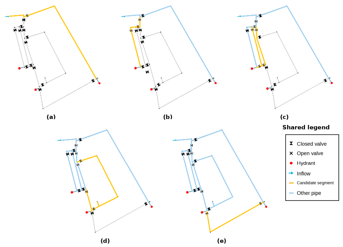
Within a selected block, candidate flushing segments are delineated using the following rules: (i) a segment remains within one existing service block; (ii) the included pipes form a connected set; (iii) the segment can be topologically isolated using installed gate valves; (iv) at least one existing hydrant or designated outlet, including a scour or washout outlet where available, is present; (v) existing isolation points and major diameter or geometry transitions are preferred as segment boundaries; and (vi) pipes of similar diameter are grouped where practicable. These rules formalize the pre-design segmentation step using the installed network configuration and define the candidate UDF configurations considered in the subsequent planning stage. Where a high-priority connected segment lacks an adequate existing outlet, the screening result identifies a location at which an additional discharge facility may warrant separate hydraulic assessment.

The resulting segments and valve–hydrant combinations are candidate configurations rather than hydraulically approved flushing operations. Before field implementation, each candidate requires conventional hydraulic and operational verification, including achievable flushing velocity, pressure response, hydrant or outlet discharge, required water volume, and valve-operating sequence. Simultaneous or sequential flushing is therefore not determined from topology or facility location alone.

The output of this stage is a finite planning inventory of pipe segments, isolation facilities, and candidate outlets that can be taken forward to detailed hydraulic analysis. This preserves the role of field expertise and utility operating judgment in final flushing design while reducing the network-wide search space that must be examined in detail.

3. Application

3.1. Study Network

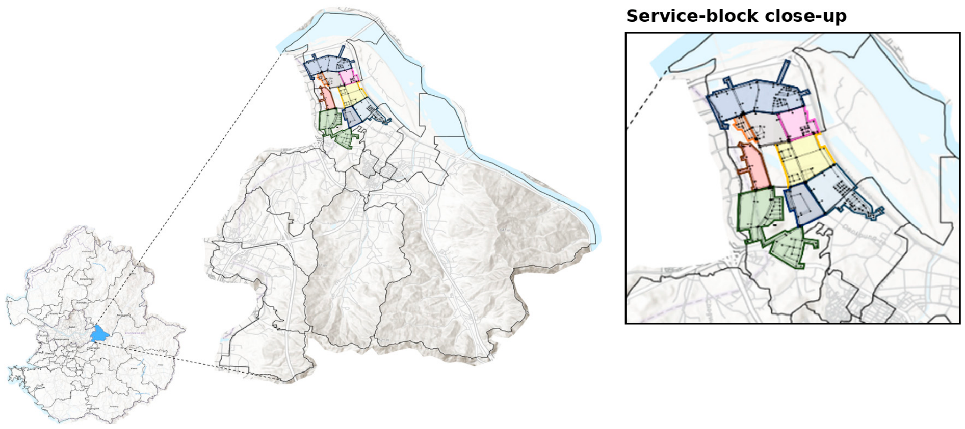
A district in City A, County G, Korea, was selected as the study area. The area experienced two water-discoloration incidents in 2018, which resulted in water-supply interruptions and subsequent flushing operations (Figure 2). The selected network spans approximately 4.95 km² and is supplied by a single reservoir with an average supply of 24,316.67 m³/d through 481 pipes and 394 junctions. Because the service area is predominantly composed of apartment complexes, domestic water demand accounts for the majority of total consumption.

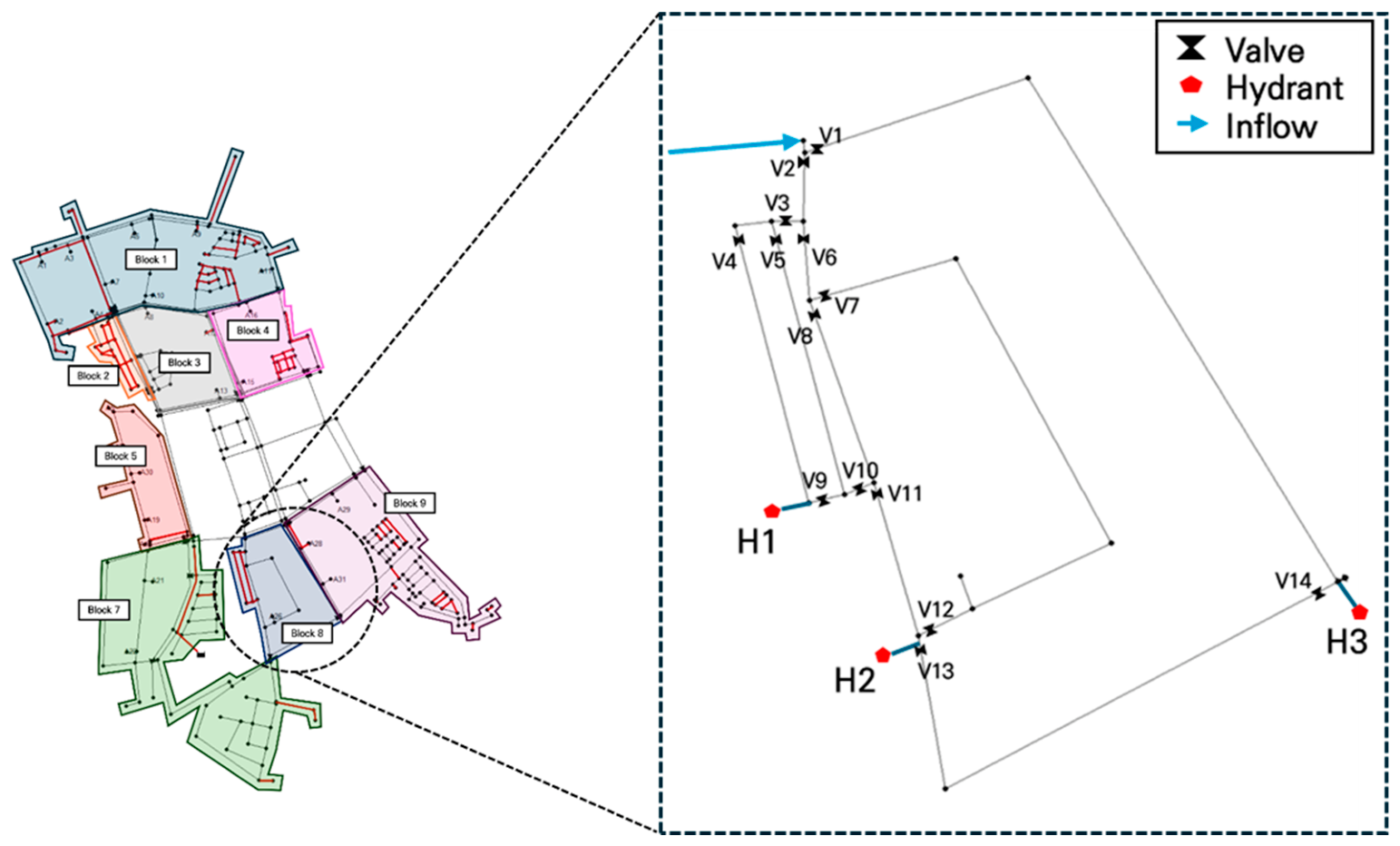
The water distribution network operates as a gravity-fed system without booster pumps and is divided into nine pre-existing service blocks. Facility records include 15 pressure-reducing valves (PRVs), 462 gate valves, 15 air-release valves, and 10 hydrants. The service-block boundaries, gate valves, and hydrants provide the operational structure used for subsequent block aggregation and candidate-segment delineation.

3.2. Basic Data Analysis

This study collected the data required to identify priority pipes and candidate flushing segments in City A, including pipe diameter, installation year, pipe length, customer demand, network topology, facility locations, and available operational information. Pipe and node geometries were constructed from GIS data and converted to an EPANET input model. Model parameters were iteratively adjusted using available operational pressure and flow observations, and the agreement between simulated and observed hydraulic conditions was reviewed before the hydraulic outputs were used to construct the DEA indicators. Detailed georeferenced network information is not disclosed because of infrastructure-security restrictions.

City A is a recently developed urban area, with most pipes installed within the previous decade. Specifically, pipe ages generally range from 6 to 11 years, while a smaller number of recently installed pipes are approximately 4 years old. The total pipe length is approximately 55,000 m, with an average diameter of approximately 170 mm. Pipe diameters range from 80 to 800 mm, and pipes with diameters of 100 mm or less account for more than half of the network.

The DEA-input and DEA-output variables were calculated under the hydraulic conditions defined for the two screening models. The sedimentation factors were derived from the 24-h EPANET simulation under normal operating conditions, whereas the detachment factors were derived by comparing the normal condition with an emergency interconnection scenario in which the supply source was switched. The detachment analysis included the effect area, velocity difference, and flow reversal defined in Section 2.1.3. Flow reversal was represented as a binary indicator (0 or 1), indicating whether a reversal occurred during source switching.

Because the variables differed in physical units and numerical ranges, min–max scaling was applied prior to DEA. In the numerical DEA matrices, the upper end of each transformed range was represented by 1, while the lower end was represented by a small positive value rather than a literal numerical zero to avoid degeneracy in the adopted DEA implementation. This numerical treatment should be distinguished from the physical meaning of the original variables. For example, a raw stagnation ratio of 0 indicates no zero-velocity reporting step, and a raw flow-reversal value of 0 indicates that no reversal occurred; their numerical representation in the DEA matrix does not imply that these events occurred. The effect-area indicator was first transformed using Equation (2) and subsequently normalized. The priority direction of the remaining variables was represented through their DEA input/output roles defined in Table 1. The same preprocessing procedure was applied consistently to all pipes.

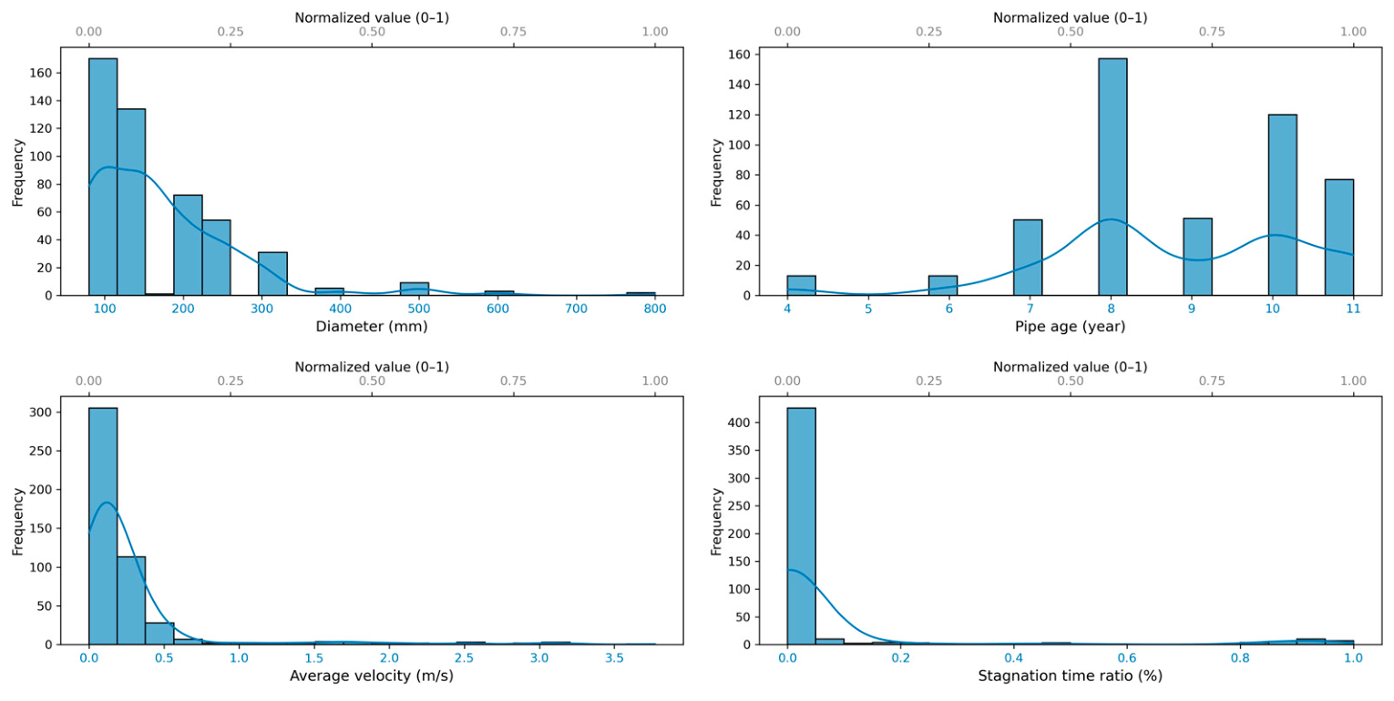
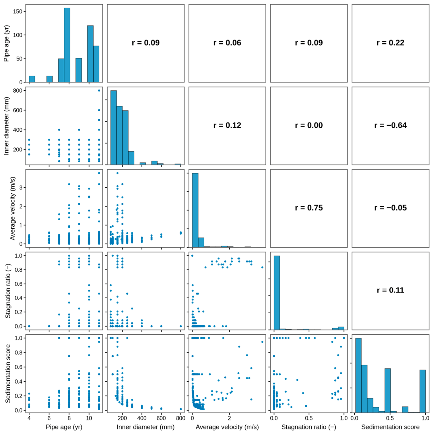
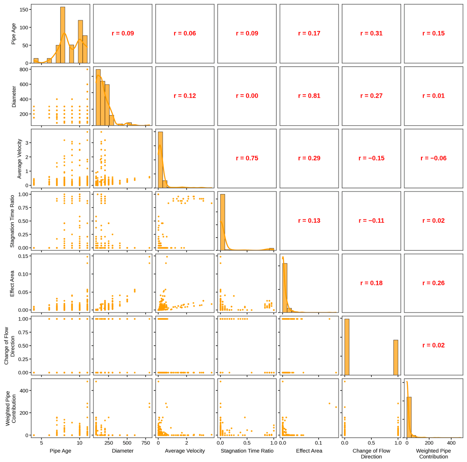
Figure 3 illustrates the distributions of the four sedimentation factors. Pipe diameters are concentrated at 200 mm or less, and pipe ages are generally distributed within a relatively narrow range. Average velocity is strongly skewed toward low values, although several pipes experience substantially higher velocities. Stagnation time ratio is zero or small for most pipes, while a limited subset experiences prolonged no-flow periods. These distributions show that the structural and hydraulic indicators have markedly different empirical characteristics before numerical preprocessing for DEA.

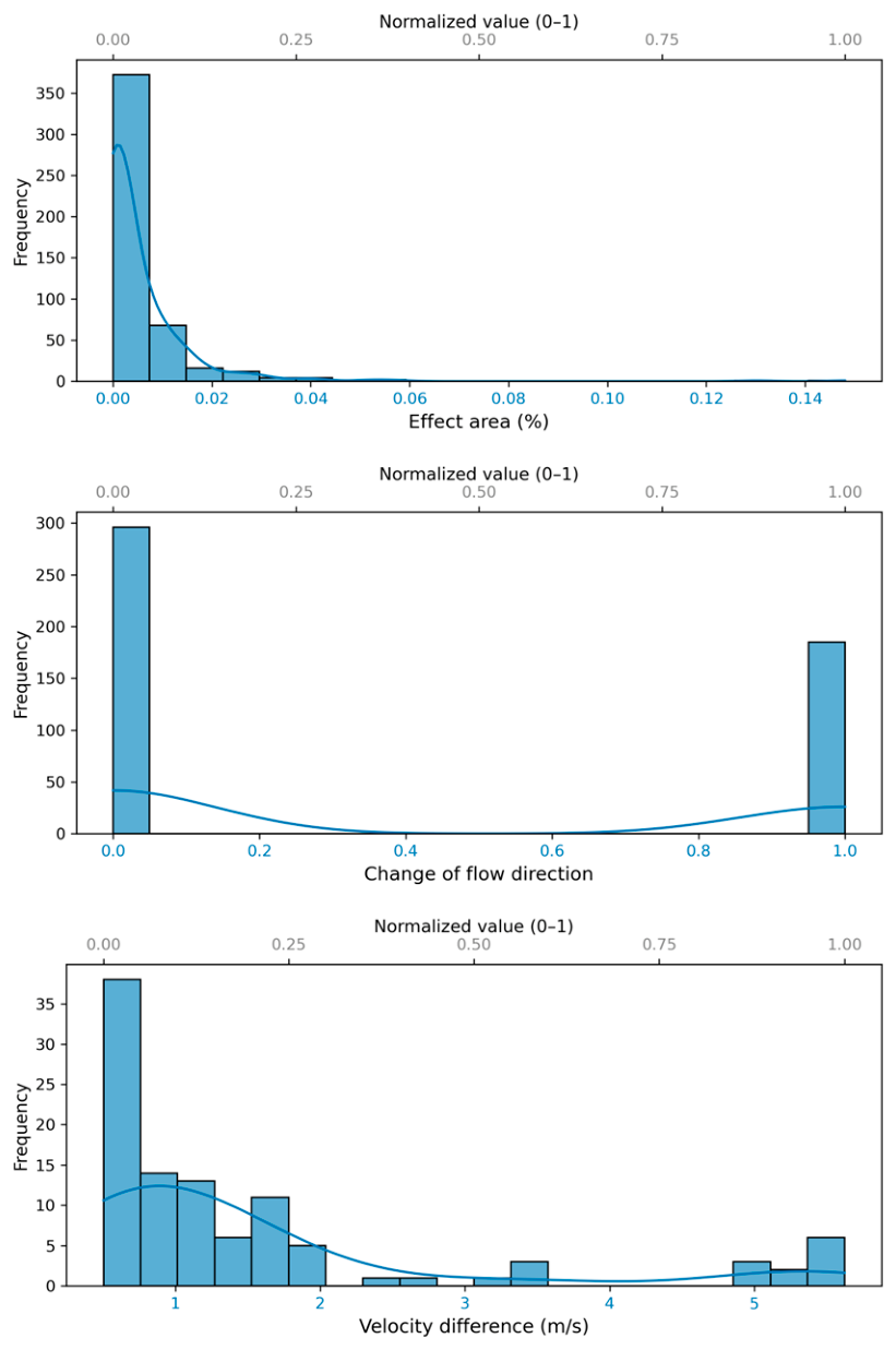
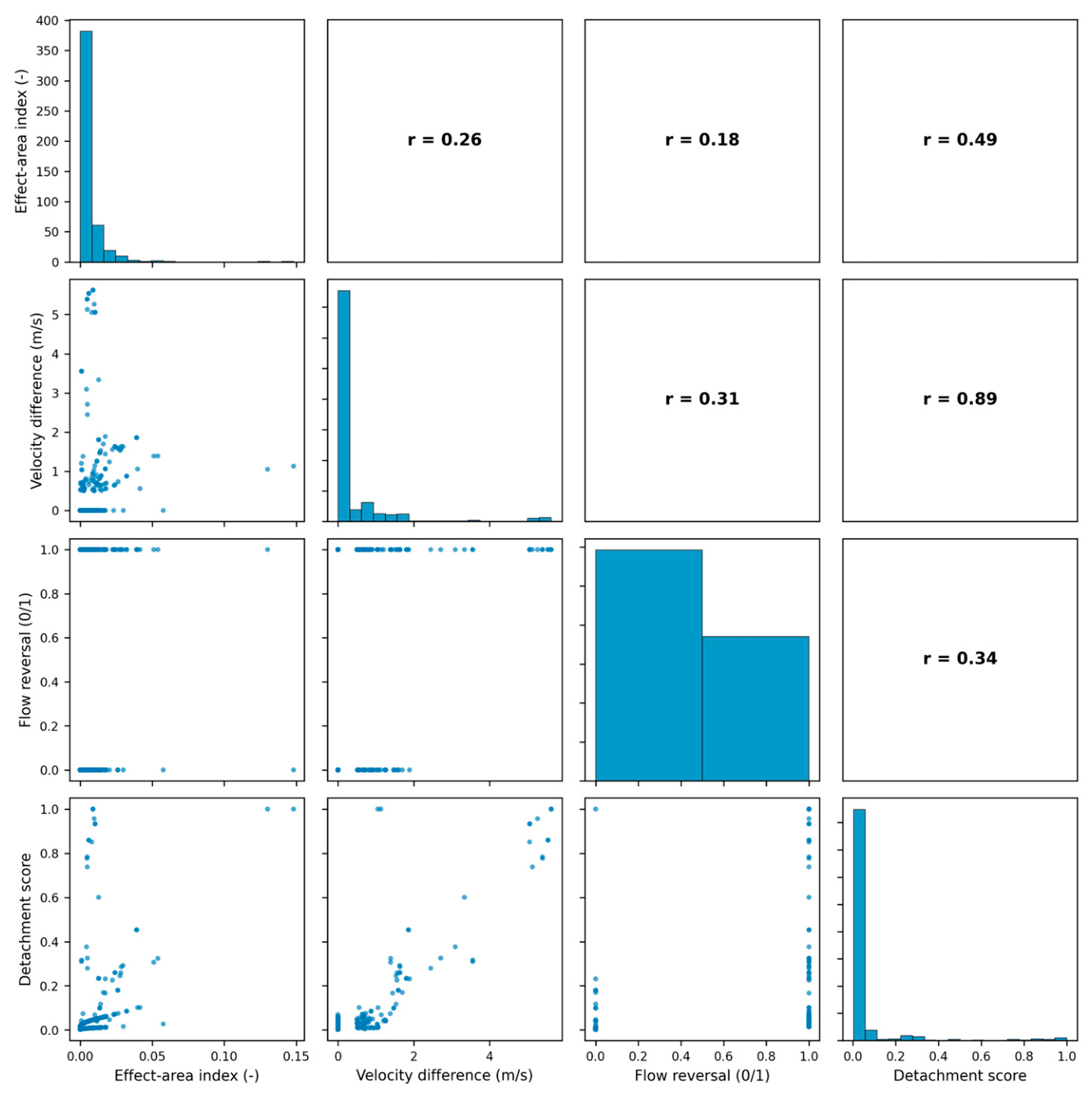
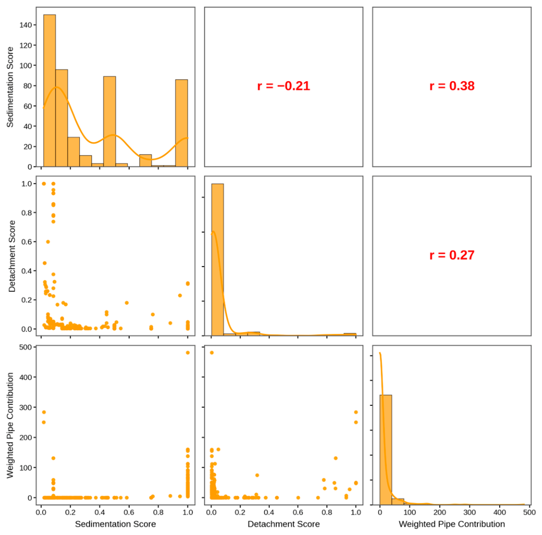
Figure 4 shows the distributions of the three detachment indicators. The raw effect-area proxy is strongly right-skewed, flow reversal is binary, and velocity difference contains many zero values because changes below 0.5 m/s are screened out by the adopted definition. A smaller subset of pipes experiences substantially larger velocity changes or flow reversal under source switching. The three variables therefore describe different aspects of the same operational disturbance and are evaluated jointly in the detachment DEA model.

The resulting dataset therefore incorporates both the physical characteristics of the network and the hydraulic conditions obtained under the normal and source-switching scenarios. Based on these data, the following section evaluates the relative sedimentation and detachment priorities of the pipes and their subsequent aggregation at the service-block level.

4. Results

4.1. Analysis of High-Risk Pipes and Determination of Risk Blocks

Section 4.1 interprets the two DEA scores at the pipe scale and then follows the selected pipe classes into service-block aggregation. The pairwise correlations are used to describe the relationships between the selected indicators and the resulting DEA scores within the analyzed dataset. Because these indicators are themselves included in the DEA models, the correlations are interpreted as descriptive diagnostics rather than as independent validation of sediment accumulation or detachment.

4.1.1. Analysis of Sedimentation Risk

The sedimentation model jointly evaluates pipe diameter, average velocity, pipe age, and stagnation time ratio. The resulting DEA values represent relative screening priorities within the analyzed network, with higher values indicating a less favorable combination of the selected sedimentation-related conditions under the adopted orientation. Accordingly, the scores rank the pipes relative to one another; they do not quantify the mass of deposited material or the probability of a future incident.

Pipes with diameters of 100 mm or less account for approximately 54% of the network. Figure 5 shows a negative association between pipe diameter and the sedimentation score ($r=-0.64$, $p<0.001$), indicating that smaller-diameter pipes tend to receive higher relative scores in the present dataset. However, pipes with similar diameters are distributed over a broad range of DEA scores because diameter is evaluated jointly with velocity, age, and stagnation. The observed relationship therefore indicates strong diameter-related discrimination in this network rather than a deterministic relationship between pipe diameter and sediment accumulation.

Approximately 62% of all pipes had average velocities within the range of 0.3–0.5 m/s, while some pipes exhibited extremely low velocities below 0.1 m/s. The correlation between average velocity and the sedimentation score is weakly negative ($r=-0.05$), indicating that low daily mean velocity alone does not reproduce the DEA ordering. Average velocity and stagnation time ratio are positively correlated in the present dataset ($r=0.75$). These two indicators nevertheless represent different characteristics of the 24-h hydraulic series: a pipe can experience several zero-flow periods while maintaining a comparatively high daily mean velocity when velocities during the remaining active-flow periods are sufficiently large. Their simultaneous use therefore retains information on both the overall flow level and intermittent stagnation.

Pipe age shows a modest positive correlation with the sedimentation score ($r=0.22$). Pipe age is an installation-history variable and is not expected to have a monotonic relationship with hydraulic velocity, which is governed by network topology, demand allocation, pipe diameter, supply path, and operational conditions. In addition, the relatively narrow age range of the case-study network limits the discriminatory power of age alone.

Stagnation time ratio is also positively associated with the sedimentation score in the present dataset ($r=0.11$, $p<0.05$). Because the ratio represents the proportion of zero-flow reporting steps, a higher value identifies pipes that experience more frequent or prolonged periods of no flow. The magnitude of the correlation is relatively small, but stagnation provides temporal information that is not represented directly by the daily average velocity.

Figure 5 therefore shows that the DEA ordering cannot be reproduced completely by any single indicator. Although diameter exhibits the strongest individual association with the sedimentation score, pipes near the priority frontier occur under different combinations of diameter, velocity, age, and stagnation. This pattern was further examined through indicator-omission analysis. Removing average velocity, stagnation time ratio, or pipe age retained 85, 83, and 81 of the baseline 88 priority pipes, respectively, whereas removing pipe diameter retained 39. These results confirm that diameter is a strong discriminator in the present network, while the other structural and hydraulic indicators provide additional information that affects the composition and ordering of the selected pipe set. The result should therefore be interpreted as a dataset-specific characteristic of the multi-indicator screening model rather than as evidence that diameter alone determines sediment accumulation.

Applying the adopted classification to the pipe-level DEA output identified 88 sedimentation-priority pipes: 10 Rank 1, 7 Rank 2, 68 Rank 3, and 3 Rank 4 pipes. The remaining 393 pipes were below the strict Rank 4 screening boundary. These classified pipes are carried forward to the service-block aggregation stage, where the pipe-level priorities are combined with pipe length and spatial block membership.

Taken together, the sedimentation results indicate that the proposed DEA model provides a structured means of evaluating the combined structural and hydraulic conditions of the pipes without imposing one common analyst-defined weighting vector. The resulting score is used as a relative screening layer for subsequent block-level planning, while detailed maintenance decisions remain dependent on hydraulic feasibility, field observations, and utility operating judgment.

4.1.2. Analysis of Detachment Risk

The detachment model evaluates the hydraulic disturbance associated with the source-switching scenario together with the effect-area proxy. Its purpose is to identify pipes that become relatively prominent under the specified operational change, rather than to estimate the probability or mass of sediment release.

Velocity difference has the strongest association with the detachment score ($r=0.89$; Figure 6), followed by the effect-area proxy ($r=0.49$) and flow reversal ($r=0.34$). This result indicates that the relative detachment score is most strongly associated with the magnitude of the modeled hydraulic change in this scenario, while the potential influence range and directional reversal provide complementary information.

The effect-area proxy and velocity difference are moderately associated ($r=0.26$), while effect area and flow reversal show a weaker relationship ($r=0.18$), and velocity difference and flow reversal are positively associated ($r=0.31$). These relationships indicate that the three indicators are related but not interchangeable, because high values do not occur in exactly the same pipes.

Flow reversal distinguishes pipes that change flow direction under source switching from those that do not, whereas velocity difference retains the magnitude of the hydraulic change above the adopted screening level. A pipe with a large effect-area proxy does not necessarily receive a high detachment score when the associated hydraulic change is limited, and flow reversal alone does not determine the priority set.

The detachment results are therefore interpreted as scenario-specific relative priorities. They identify a small set of pipes for which the selected hydraulic-influence and disturbance indicators combine unfavorably under source switching, while the actual physical response remains dependent on the presence and condition of accumulated material and requires subsequent hydraulic and field verification.

Twelve pipes are included in the high-priority detachment set: four pipes in the upper detachment planning class and eight Rank 4 pipes. The remaining 469 pipes fall outside the retained detachment-priority classes. This selected set is carried forward separately from the sedimentation set until the service-block aggregation stage.

The sensitivity of the selected pipes to the velocity-difference screening level was also examined. The same 12 highest-priority detachment pipes were retained when the screening level was increased from 0.5 to 0.7, 1.0, 1.5, and 2.0 m/s. At 1.5 m/s, one additional pipe exceeded the 0.75 DEA screening boundary, although the composition of the leading 12 pipes remained unchanged. This result indicates that the principal detachment candidates are stable over the tested range, while the total number of pipes exceeding the screening boundary can vary slightly with the adopted threshold.

Indicator-omission analysis further showed that removing flow reversal retained 11 of the baseline 12 priority pipes, whereas removing velocity difference retained only two in the fixed-size top-12 comparison. This difference indicates that velocity difference provides the strongest discrimination among the highest-priority detachment pipes in the present scenario, while flow reversal contributes complementary directional information.

The pairwise plots are used to explain the structure of the detachment-screening results rather than to establish independent predictive validity. Together with the sensitivity analyses, they show how the three indicators contribute to the relative prioritization of pipes under the specified source-switching condition.

The practical role of the detachment model is therefore to focus subsequent planning on pipes that experience substantial hydraulic changes and/or comparatively large potential influence under source switching, thereby providing a manageable set of locations for subsequent block-level and hydraulic assessment.

4.1.3. Results of High-Risk Block Assessment

Table 2. Planning classes, class coefficients, and number of pipes.

Planning Class	Classification Criterion	Class Coefficient	Number of Pipes
			Sedimentation	Detachment
Rank 1	1++	1	10	0
Rank 2	1+	0.8	7	0
Rank 3	1−/upper detachment planning class	0.5	68	4
Rank 4	0.75 < θ < 1.0	0.3	3	8
Below Rank 4	θ ≤ 0.75	0	393	469

Note: The 1++, 1+, and 1− classifications refer to the sedimentation slack-based classification. The four pipes retained in the upper detachment planning class are assigned the Rank 3 coefficient for block aggregation.

summarizes the pipe classes used for service-block aggregation. Under the sedimentation analysis, 10 pipes are classified as Rank 1, 7 as Rank 2, 68 as Rank 3, and 3 as Rank 4, with 393 pipes below the Rank 4 boundary. Under the detachment analysis, four pipes are assigned to Rank 3 and eight to Rank 4, with 469 pipes below the boundary. Thus, 88 sedimentation-priority pipes and 12 detachment-priority pipes are carried forward to block assessment.

Table 3. Cumulative and length-normalized service-block priority results.

Block	Cumulative Priority Score	Cumulative Rank	Priority Intensity	Intensity Rank
1	2083.16	1	0.182	2
2	704.55	3	0.334	1
3	6.00	8	0.001	8
4	520.26	4	0.139	3
5	112.80	7	0.034	7
6	0.00	9	0.000	9
7	984.23	2	0.089	5
8	386.35	5	0.092	4
9	269.94	6	0.035	6

presents the service-block priority results obtained by combining the pipe classes with pipe length according to Equations (9) and (10). Block 1 has the highest cumulative priority score (2083.16), followed by Blocks 7 (984.23), 2 (704.55), and 4 (520.26). Blocks 8 and 9 form the next tier, while Blocks 5, 3, and 6 have substantially lower cumulative values.

To distinguish the cumulative extent of priority pipes from their concentration within blocks of different sizes, Table 3 also presents the length-normalized priority intensity defined in Equation (11). While Block 1 has the highest cumulative priority, Block 2 has the highest normalized intensity. Thus, the two measures provide complementary information: the cumulative score emphasizes the overall length-weighted maintenance priority within a block, whereas the normalized intensity indicates how strongly priority-pipe contributions are concentrated relative to the total pipe length of that block.

Priority pipes are not distributed uniformly across the nine service blocks. The block measures therefore provide a planning-scale description of the cumulative extent and the relative concentration of classified priority pipes within each block.

Figure 7 provides a descriptive view of the relationships among pipe age, diameter, average velocity, stagnation time ratio, effect area, velocity difference, flow reversal, and the length-weighted pipe contribution $P_i$ used for service-block aggregation.

Pipe age has a correlation of 0.15 with $P_i$, whereas stagnation time ratio has only a weak correlation of 0.02. Average velocity and stagnation time ratio are positively correlated in the analyzed dataset ($r=0.75$). As discussed in Section 4.1.1, these two variables characterize different aspects of an intermittent 24-h velocity series; periods of zero flow can coexist with comparatively high velocities during the remaining active-flow periods.

Pipe diameter has only a very weak association with $P_i$($r=0.01$), even though it is more strongly associated with the sedimentation score ($r=-0.64$). Average velocity also has a weak association with $P_i$($r=-0.06$). These differences illustrate that the length-weighted contribution used for block aggregation is not a simple linear surrogate for any single raw indicator but reflects the preceding DEA classification together with the pipe length.

The effect-area proxy has a weak-to-moderate positive association with $P_i$($r=0.26$), while flow reversal has only a weak association ($r=0.02$). These correlations describe the structure of the analyzed dataset and the subsequent aggregation procedure rather than independent physical effects of the individual indicators.

Because $P_i$ is constructed from the post-DEA class assignments and pipe length, the correlations in Figure 7 are used primarily to describe how the screening variables relate to the quantity subsequently accumulated at the block level. Relationships between the sedimentation and detachment DEA scores and $P_i$ are shown separately in Figure 8.

Figure 8 compares the sedimentation score, detachment score, and length-weighted pipe contribution. Sedimentation and detachment scores are weakly negatively associated ($r=-0.21$), indicating that pipes emphasized by the two screening mechanisms are not necessarily the same. The sedimentation score has a positive association with $P_i$($r=0.38$), while the detachment score has a weaker positive association ($r=0.27$). Because $P_i$ is calculated after DEA classification and incorporates pipe length, these relationships describe the transition from pipe-level screening to service-block aggregation rather than predictive relationships with observed water-quality incidents.

The pairwise distributions therefore support retaining sedimentation and detachment as separate screening mechanisms through the pipe-level stage before their class-based contributions are combined for service-block prioritization. Most pipes have relatively low sedimentation and detachment scores, whereas a smaller subset approaches the priority frontier and contributes to the length-weighted block scores.

The block-level results further show that these contributions are spatially uneven across the network. Blocks 1, 7, 2, and 4 have the highest cumulative priority scores, whereas the normalized results show that Block 2 contains the greatest concentration of priority contribution per unit pipe length. This distinction allows the cumulative extent of priority pipes and their within-block concentration to be considered separately when selecting areas for more detailed flushing assessment.

Overall, the block assessment translates the pipe-level relative classifications into the operational service-block units used by the utility. The resulting block measures support planning decisions rather than failure prediction.

4.2. Candidate Flushing Planning for a Representative Block

Block 8 is used as a representative case to demonstrate how a prioritized service block can be translated into candidate flushing segments. It ranks fifth in the cumulative block assessment and fourth in the length-normalized priority intensity, indicating a meaningful concentration of priority pipes without being the highest-ranked block in the network. More importantly, its existing valve–hydrant configuration provides a clear example for illustrating the segmentation procedure because several connected pipe groups can be delineated using different combinations of the installed facilities. Selection of Block 8 for demonstration does not alter the network-wide priority ranking.

For this purpose, the internal layout of Block 8 was mapped, and the identifiers of the major existing facilities, including hydrants (H1–H3) and gate valves (V1–V14), are shown in Figure 9. These facilities are treated as fixed operational constraints for candidate-segment delineation rather than as optimized locations.

In the next stage, Block 8 was subdivided into five candidate segments (a–e) using the structural network layout and the locations of the existing hydrants and gate valves. Each candidate forms a connected pipe set that can be considered for isolation and includes an existing hydrant as a potential flushing outlet. The segment boundaries therefore represent planning-level candidate UDF configurations rather than hydraulically approved operating zones.

Where multiple topologically feasible boundary locations existed, existing isolation points and major diameter or geometry transitions were preferred, while pipes of similar diameter were grouped where practicable. Segment pipe length, diameter, candidate valve set, and hydrant location were compiled to support subsequent engineering review (Figure 10).

Table 4. Candidate flushing configurations by segment in Block 8.

	Segment (a)	Segment (b)	Segment (c)	Segment (d)	Segment (e)
Candidate valve set	V1	V2, V3, V4	V2, V3, V5, V6, V9, V10	V2, V6, V7, V8, V11, V12	V2, V6, V8, V11, V13, V14
Pipe diameter (mm)	250, 300	80, 250	80, 250	80, 200, 250	250
Segment length (m)	892.4	465.8	678.9	928.6	633.7
Candidate hydrant outlet	H3	H1	H1	H2	H3

lists the candidate segments together with the corresponding valve sets, designated hydrant outlets, pipe diameters, and segment lengths. The table functions as a pre-design inventory that identifies the pipe and facility combinations to be taken forward to detailed hydraulic assessment. Final valve operating states, flushing discharge, flushing duration, restoration sequence, pressure response, and other site-specific operating restrictions are determined only after the candidate set has been established.

The candidate configurations for Block 8 are not intended to replace hydraulic simulation. Network structure and existing facility locations are used to reduce the number of configurations that require detailed review; achievable flushing velocity, pressure response, hydrant discharge, water volume, and safe valve operation must be confirmed before field implementation. Any simultaneous or sequential operation is therefore determined only after hydraulic assessment of the candidate segments.

The complete planning sequence consists of pipe-level DEA screening, service-block prioritization, facility-constrained candidate-segment delineation, and subsequent hydraulic verification. The five configurations derived for Block 8 therefore represent candidate UDF plans that define where detailed hydraulic evaluation should be concentrated, rather than final flushing operations. This separation preserves the role of hydraulic modeling and field judgment in the final design while using the DEA results to focus that effort on a smaller and explicitly defined set of locations.

5. Discussion

5.1. DEA Model Specification and Indicator Contributions

The pipe-level results should be interpreted in relation to the DEA formulation adopted for the screening problem. The efficiency score used in this study does not represent conventional operational efficiency or a calibrated probability of a water-quality event. Instead, the input and output variables are oriented so that pipes exhibiting less favorable sedimentation- or detachment-related conditions approach the DEA frontier. The resulting values therefore provide relative screening priorities within the analyzed network and under the specified model structure.

The principal robustness checks are summarized in

Table 5. Summary of the principal pipe-level robustness analyses.

Sensitivity Check	Sedimentation	Detachment	Main Interpretation
Alternative DEA form	CCR-I: ρ = 0.932; top-88 overlap = 74/88. BCC-O: 214 pipes above 0.75.	CCR-I: ρ = 0.986; top-12 overlap = 2/12. BCC-O: 186-pipe frontier.	BCC-I retains comparatively selective screening under the adopted orientation.
Indicator omission	Diameter removal: ρ = 0.508; overlap = 39/88.	ΔV removal: overlap = 2/12; flow-reversal removal: 11/12.	The strongest discriminators differ between the two screening components.
ΔV threshold	—	Top-12 retained for thresholds from 0.5 to 2.0 m/s.	Principal detachment candidates are stable within the tested upward range.
Equal-weight WSM	ρ = 0.580; overlap = 57/88.	ρ = 0.982; overlap = 11/12.	Common-weight and DEA rankings differ more strongly for sedimentation.
AR 0.1–10	ρ = 0.984; overlap = 76/88.	ρ = 0.999; overlap = 12/12.	Broad ranking structure remains comparatively stable under moderate weight restrictions.

BCC-I, input-oriented Banker–Charnes–Cooper model; CCR-I, input-oriented Charnes–Cooper–Rhodes model; BCC-O, output-oriented BCC model; ΔV, velocity difference; AR, assurance region. Detailed values are provided in Appendix A Table A1, Table A2, Table A3, Table A4, Table A5, Table A6, Table A7 and Table A8.

, while the complete model-form, effect-area, indicator-removal, preprocessing, and weight-flexibility results are provided in Appendix A. The comparison with alternative DEA formulations shows that the overall ordering can remain similar even when the number of pipes retained above the screening boundary changes substantially. Output-oriented BCC produces a much broader high-score region, particularly for the detachment model, and therefore provides less selective screening under the present indicator orientation. These results support retaining the input-oriented BCC formulation as the baseline while making clear that the selected set remains conditional on the stated model specification.

The indicator-removal results reveal different structures for the two screening components. Sedimentation priority is particularly sensitive to pipe diameter, whereas removing average velocity, stagnation ratio, or pipe age produces comparatively smaller changes in the selected set. This strong diameter-related discrimination is consistent with the empirical structure of the case-study network, in which pipe age varies over a relatively narrow range while diameter spans 80–800 mm. The result should not be interpreted as evidence that smaller pipes necessarily contain more deposited sediment. Diameter is one structural descriptor within the four-indicator model, and the hydraulic and temporal indicators continue to differentiate pipes with similar diameters.

The detachment model shows a different pattern. Removing velocity difference substantially reduces discrimination among the highest-priority pipes, whereas removal of flow reversal leaves most of the original priority set unchanged. This behavior is consistent with the strong relationship between velocity difference and the detachment score and indicates that the magnitude of the source-switching disturbance provides the principal separation among the upper-ranked pipes in this operating scenario. Effect area remains structurally important because it is the sole DEA input in the detachment model; its removal produces a degenerate input-oriented comparison rather than an ordinary leave-one-out model.

5.2. Robustness to Preprocessing, Hydraulic Screening, and DEA Weight Flexibility

The sensitivity analyses also show that numerical preprocessing is an integral part of the DEA specification rather than a neutral formatting step. The archived DEA matrices represent lower numerical endpoints using small positive values. These numerical values should be distinguished from the physical meaning of the original observations: a raw stagnation ratio of zero still denotes the absence of zero-velocity reporting steps, and a raw flow-reversal value of zero still denotes that no reversal occurred. Appendix A

Table A4. Positive numerical minima used in the archived DEA matrices.

Component	Indicator	Numerical Minimum	Encoding Rule
Sedimentation	Diameter input	0.01388889	0.5 × smallest positive exact min-max value
Sedimentation	Average velocity input	0.00132626	0.5 × smallest positive exact min-max value
Sedimentation	Stagnation output	0.02083333	0.5 × smallest positive exact min-max value
Sedimentation	Age output	0.14285714	0.5 × smallest positive exact min-max value
Detachment	Effect-area input	0.00256271	0.2 × smallest positive log-reciprocal min-max value
Detachment	Velocity-difference output	0.01788297	0.2 × smallest retained normalized value
Detachment	Flow-reversal output	0.10000000	Raw 0 represented by 0.1; raw 1 remains 1

and

Table A5. Comparison of alternative normalization schemes.

Component	Scheme	Spearman ρ	Frontier n	Score > 0.75 n	Top-k Overlap
Sedimentation	Current archived	1.000	85	88	88/88
Sedimentation	Literal-zero min-max	0.705	17	22	48/88
Sedimentation	Ratio-to-max	0.971	85	179	88/88
Sedimentation	Winsorized 1–99% min-max	0.968	102	104	73/88
Detachment	Current archived	1.000	3	12	12/12
Detachment	Literal-zero min-max	0.881	6	9	7/12
Detachment	Ratio-to-max	0.825	7	12	8/12
Detachment	Winsorized 1–99% min-max	0.811	11	12	7/12

provide the archived lower endpoints and the corresponding normalization diagnostics.

Replacing the archived positive lower endpoints with literal numerical zeros changes the sedimentation frontier and selected set substantially, whereas several positive lower-endpoint perturbations around the archived representation retain the principal priority set. The detachment model is more stable over the tested positive-endpoint range. These results support retaining the archived preprocessing convention for reproduction of the reported planning result while also showing that the numerical representation should be stated explicitly when the method is transferred to another network.

The velocity-difference screening level shows greater robustness. Raising the threshold from 0.5 to 2.0 m/s retains the same leading 12 detachment candidates, although one additional pipe crosses the DEA screening boundary at 1.5 m/s. The 0.5 m/s value is therefore an operational screening level for the source-switching analysis, not a calibrated sediment-detachment threshold. The detailed threshold results are given in Appendix A

Table A6. Upward velocity-difference threshold stress test.

Threshold (m/s)	Retained ΔV n	Spearman ρ	Score > 0.75 n	Top-12 Overlap
0.50	104	1.000	12	12/12
0.70	73	1.000	12	12/12
1.00	52	1.000	12	12/12
1.50	33	0.994	13	12/12
2.00	17	0.986	12	12/12

.

A further methodological issue concerns the flexibility of the endogenous DEA multipliers. The stored unrestricted solutions are sparse for several variables, which confirms that optimized DEA multipliers do not represent universal physical-importance coefficients. The assurance-region (AR) tests nevertheless retain high whole-ranking agreement with the baseline, particularly for detachment. Sedimentation becomes progressively more selective as the allowable weight-ratio interval narrows. Because no externally calibrated weight-ratio bounds are available for the study network, the unrestricted BCC formulation is retained as the baseline, while the assurance-region and multiplier results in Appendix A

Table A8. Exploratory assurance-region sensitivity.

Component	Weight-Ratio Interval	Spearman ρ	Frontier n	Score > 0.75 n	Top-k Overlap
Sedimentation	0.1–10	0.984	15	73	76/88
Detachment	0.1–10	0.999	3	12	12/12
Sedimentation	0.2–5	0.976	15	60	76/88
Detachment	0.2–5	0.996	3	12	12/12
Sedimentation	0.5–2	0.948	13	40	66/88
Detachment	0.5–2	0.992	3	12	12/12

and

Table A9. Summary of stored unrestricted optimal multiplier solutions.

Component	Multiplier	Zero n	Zero (%)	Median	Maximum
Sedimentation	Diameter input	34	7.1	10.286	72.000
Sedimentation	Average velocity input	342	71.1	0.000	754.000
Sedimentation	Stagnation output	450	93.6	0.000	3.725
Sedimentation	Age output	422	87.7	0.000	19.427
Detachment	Effect-area input	0	0.0	2.028	390.213
Detachment	Velocity-difference output	436	90.6	0.000	3.268
Detachment	Flow-reversal output	298	62.0	0.000	0.889

are used to identify the sensitivity of that choice. Stored cross-efficiency results were also reviewed as a secondary diagnostic; because peer appraisal can depend on alternative optimal multipliers and secondary-objective choices, cross-efficiency was not used as the primary robustness criterion.

5.3. Comparison with Common-Weight Prioritization and Robustness of Service-Block Decisions

The use of DEA in this study is motivated in part by the absence of an externally established common weighting vector for the selected structural and hydraulic indicators. Equal-weight weighted-sum method (WSM) and TOPSIS were therefore evaluated as structural comparators using the same available indicators and aligned priority directions. These comparisons are not tests of predictive superiority because no independent pipe-level observations of sediment mass, discoloration response, or flushing outcome are available as ground truth. Instead, they show how the screening outcome changes when a common weighting structure is imposed.

The sedimentation ranking differs substantially between DEA and the equal-weight alternatives, whereas the detachment rankings show much greater agreement. At the service-block scale, however, the main planning decisions are more stable than the individual pipe rankings. The key block-level results are summarized in

Table 6. Summary of service-block robustness and planning interpretation.

Sensitivity Check	Principal Result	Planning Interpretation
Baseline cumulative priority	1 > 7 > 2 > 4 > 8 > 9 > 5 > 3 > 6	Block 1 has the largest total length-weighted priority.
Length-normalized intensity	2 > 1 > 4 > 8 > 7 > 9 > 5 > 3 > 6	Block 2 has the greatest concentration of priority contribution.
Pipe-length exponent, α = 0–1	Leading set {1, 2, 4, 7} retained; internal order changes.	Pipe length affects ordering within the leading group but not its membership.
Alternative class coefficients	Leading block group retained; only middle ranks change in one deterministic case.	Block prioritization is not driven by one coefficient spacing.
Score cut-off, 0.75–0.95	Complete baseline block order retained.	More restrictive screening leaves the block order unchanged.
Score cut-off, 0.60–0.70	Block 9 moves above Block 4.	Middle-ranked blocks are more sensitive when near-threshold pipes are added.
Equal-weight WSM propagation	Leading set {1, 2, 4, 7} retained.	Block-level decisions are more stable than the underlying pipe ranking.

, and the complete common-weight, pipe-length, class-coefficient, and score-cutoff results are provided in Appendix A

Table A7. Equal-weight pipe-level and matched-cardinality block comparisons.

Component/Level	Comparator	Spearman ρ	Top-k Overlap	Block Order/Note
Sedimentation pipe	Equal-weight WSM	0.580	57/88	—
Sedimentation pipe	Equal-weight TOPSIS	0.445	37/88	—
Detachment pipe	Equal-weight WSM	0.982	11/12	—
Detachment pipe	Equal-weight TOPSIS	0.992	10/12	—
Block	DEA baseline	1.000	4/4 top blocks	1, 7, 2, 4, 8, 9, 5, 3, 6
Block	Equal-weight WSM	0.833	4/4 top blocks	1, 4, 2, 7, 9, 5, 3, 8, 6
Block	Equal-weight TOPSIS	0.533	3/4 top blocks	1, 4, 7, 3, 9, 5, 2, 6, 8

,

Table A10. Service-block ranking under alternative pipe-length exponents.

Length Exponent α	Block Order	Spearman ρ
0.00	1, 2, 4, 7, 9, 8, 5, 3, 6	0.933
0.25	1, 2, 4, 7, 8, 9, 5, 3, 6	0.950
0.50	1, 2, 4, 7, 8, 9, 5, 3, 6	0.950
0.75	1, 7, 2, 4, 8, 9, 5, 3, 6	1.000
1.00	1, 7, 2, 4, 8, 9, 5, 3, 6	1.000

,

Table A11. Service-block ranking under alternative post-DEA class coefficients.

Specification	Block Order	Spearman ρ
Baseline 1.0/0.8/0.5/0.3	1, 7, 2, 4, 8, 9, 5, 3, 6	1.000
1.0/0.8/0.6/0.4	1, 7, 2, 4, 8, 9, 5, 3, 6	1.000
2.0/1.0/0.5/0.25	1, 7, 2, 4, 9, 8, 5, 3, 6	0.983
4.0/3.0/2.0/1.0	1, 7, 2, 4, 8, 9, 5, 3, 6	1.000
Four upper detachment pipes → Rank 1	1, 7, 2, 4, 8, 9, 5, 3, 6	1.000
Four upper detachment pipes → Rank 2	1, 7, 2, 4, 8, 9, 5, 3, 6	1.000

and

Table A12. Service-block ranking under alternative DEA score cut-offs.

Cut-Off	Sedimentation n	Detachment n	Block Order	Spearman ρ
0.60	100	14	1, 7, 2, 9, 4, 8, 5, 3, 6	0.950
0.65	100	13	1, 7, 2, 9, 4, 8, 5, 3, 6	0.950
0.70	100	13	1, 7, 2, 9, 4, 8, 5, 3, 6	0.950
0.75	88	12	1, 7, 2, 4, 8, 9, 5, 3, 6	1.000
0.80	87	10	1, 7, 2, 4, 8, 9, 5, 3, 6	1.000
0.85	87	10	1, 7, 2, 4, 8, 9, 5, 3, 6	1.000
0.90	86	7	1, 7, 2, 4, 8, 9, 5, 3, 6	1.000
0.95	85	5	1, 7, 2, 4, 8, 9, 5, 3, 6	1.000

.

The pipe-length analysis provides a clear example of this distinction. When the influence of pipe length is reduced or removed, Block 7 moves downward and Blocks 2 and 4 become more prominent, yet Blocks 1, 2, 4, and 7 remain the leading set throughout the deterministic length-exponent cases. Thus, length weighting affects the internal order of the leading blocks but does not solely determine which blocks emerge as principal candidates. A similar pattern is observed for alternative post-DEA class coefficients, for which the leading block group remains stable and only middle-ranked blocks exchange positions under one tested spacing.

The screening cut-off has a somewhat different effect. More restrictive cut-offs retain the complete baseline block order, whereas lowering the cut-off introduces additional near-threshold pipes and moves Block 9 above Block 4. This result is operationally useful because it distinguishes decisions that remain stable across reasonable planning choices from those that depend more strongly on the breadth of the screening set.

The cumulative and normalized block measures should likewise be interpreted as complementary. Block 1 contains the largest cumulative priority and therefore represents the greatest total extent of length-weighted priority pipe, whereas Block 2 has the highest normalized priority intensity and therefore represents the greatest concentration of priority contribution relative to total block length. These two measures support different maintenance decisions: one emphasizes the overall extent of attention required, while the other identifies areas where priority conditions are concentrated within a comparatively small network length.

5.4. Practical Implications and Limitations

The principal practical contribution of the framework is the translation of a network-wide screening problem into a sequence of pipe-, block-, and segment-level decisions. The DEA analysis reduces the full 481-pipe network to a smaller set of pipes requiring closer attention, while the subsequent block aggregation translates those classifications into the pre-existing service-block structure used by the utility. Candidate UDF configurations are then defined using installed isolation and discharge facilities rather than by introducing optimized or hypothetical network components.

The Block 8 application illustrates this transition. Block 8 is not the highest-ranked block in cumulative priority, but it ranks fifth cumulatively and fourth in normalized priority intensity. More importantly for demonstration of the procedure, its valve-hydrant configuration permits several distinct connected pipe groups to be delineated using the existing facilities. The five configurations identified in Section 4.2 should therefore be interpreted as representative candidate UDF plans rather than as evidence that Block 8 should necessarily be treated before all higher-ranked blocks. The network-wide priority assessment and the candidate-segment demonstration serve different roles within the overall planning procedure.

The candidate configurations do not replace conventional hydraulic design. Topological connectivity, isolation-valve availability, hydrant location, and pipe geometry are sufficient to define a manageable set of candidate segments, but they do not demonstrate that the required flushing velocity can be achieved while maintaining acceptable pressures. Final implementation requires additional verification of flushing velocity, pressure response, outlet discharge, required water volume, valve-operating sequence, restoration procedure, and field-operability constraints. The present framework therefore identifies where detailed engineering analysis should be concentrated rather than prescribing the final operating conditions.

The interpretation of the results is further limited by the available evidence. The case study is based on one utility-scale network and does not include pipe-level observations of deposited sediment mass, geocoded discoloration or turbidity responses, field flushing outcomes, or a contemporaneous expert-ranked pipe list that could be used as independent ground truth. The reported DEA scores are therefore relative planning indicators within the analyzed network, not calibrated failure probabilities. The historical discoloration incidents provide operational context for the study area, but the available archive does not support a defensible pipe-level spatial validation against those events.

Standard hydraulic benchmark networks also do not provide an equivalent validation environment for the present planning problem because they generally lack the combined installation-age, operational switching, service-block, gate-valve, hydrant, and field-response information required by the workflow. Synthetic assignment of these attributes could demonstrate numerical execution but would not constitute equivalent utility-scale validation. The sensitivity analyses nevertheless identify which planning outputs remain comparatively stable and which depend more strongly on model specification, preprocessing, or screening conventions, thereby providing a practical basis for future application to additional data-rich utility systems.

6. Conclusions

This study developed a DEA-based planning framework to support flushing prioritization in water distribution networks by linking pipe-level screening, service-block prioritization, and candidate flushing-segment planning. Seven structural and hydraulic indicators were evaluated using separate sedimentation and detachment models based on an input-oriented BCC DEA formulation. The DEA scores were used as relative screening priorities within the analyzed network, thereby allowing heterogeneous pipe information to be evaluated without prescribing a single common expert-defined weighting vector.

Application to the 481-pipe case-study network identified 88 sedimentation-priority pipes and 12 detachment-priority pipes. Because the two sets did not overlap, 100 unique pipes, corresponding to 20.8% of the network, were included in at least one priority set. The resulting pipe classes were combined with pipe length and aggregated within the nine pre-existing service blocks. Blocks 1, 7, 2, and 4 received the highest cumulative priorities, while the length-normalized analysis identified Block 2 as having the greatest concentration of priority contribution. These two block measures therefore provide complementary information on the overall extent and spatial concentration of maintenance priority.

The block-level results were subsequently connected to the existing valve and hydrant configuration to establish candidate UDF plans. Five candidate flushing segments were delineated in Block 8 as a representative case, demonstrating how network-wide screening can be translated into physically defined pipe and facility combinations for subsequent engineering assessment. The sensitivity analyses further showed that the principal planning decisions were comparatively stable under several alternative assumptions. In particular, the leading service-block group remained consistent under changes in pipe-length weighting and class coefficients, while the leading detachment candidates were retained across the tested velocity-difference screening levels. At the same time, the sedimentation results were more sensitive to indicator selection, preprocessing, and DEA weight restrictions, emphasizing the need to interpret the resulting priorities within the stated model specification.

The proposed framework is therefore intended to identify where detailed flushing assessment should begin rather than to replace conventional hydraulic design. Candidate segments must still be evaluated with respect to achievable flushing velocity, pressure response, outlet discharge, required water volume, valve-operating sequence, and field conditions before implementation. In addition, the present study is based on a single utility-scale network and does not include pipe-level observations of deposited sediment mass, turbidity response, or field flushing performance as independent validation data. Future studies should apply the framework to additional data-rich utility systems, link the relative priorities with field water-quality and flushing observations, and evaluate alternative prioritization structures using comparable input and outcome data.