Spatiotemporal Prediction Algorithm for Groundwater Quality Under Multi-Indicator Coupling Constraints

Abstract

Spatiotemporal prediction of groundwater quality is of great significance for regional water environmental safety assessment, pollution risk identification, and urban groundwater resource management. To address the difficulty of existing methods in simultaneously characterizing multi-indicator coupling relationships, temporal evolution processes, and spatial heterogeneity, this study proposes a spatiotemporal groundwater quality prediction model under multi-indicator coupling constraints. First, indicators including dissolved oxygen, total nitrogen, electrical conductivity, dissolved organic carbon, pH, permanganate index, and total phosphorus are uniformly mapped into a risk space to construct an integrated groundwater quality risk index. Then, based on monthly groundwater monitoring data from Yiyang City during 2000–2023, continuous regional grid sequences are generated. In terms of model design, the Temporal Difference Interaction Module (TDIM) is introduced to enhance multi-scale temporal variation modeling, Region-Guided Feature Modulation (RGFM) is used to strengthen regional heterogeneity representation, and Spatiotemporal Boundary-Aware Loss (STB Loss) is adopted to maintain spatiotemporal boundary consistency. The experimental results show that the proposed method achieves a Structural Similarity Index Measure (SSIM) of $0.9814\pm 0.0085$, a Peak Signal-to-Noise Ratio (PSNR) of $40.47\pm 2.19$, a Mean Absolute Error (MAE) of $2.80\times {10}^{-3}\pm 1.50\times {10}^{-3}$, and a Root Mean Square Error (RMSE) of $9.70\times {10}^{-3}\pm 2.69\times {10}^{-3}$, outperforming comparison models overall and providing effective support for dynamic groundwater quality prediction and water environmental safety assessment.

1. Introduction

Groundwater is an important basic resource for maintaining regional water supply security, ecological stability, and sustainable urban development [1]. Its quality changes are directly related to domestic water use, agricultural production, industrial utilization, and the safety of urban underground space development. With the acceleration of urbanization, changes in land use patterns, and the intensification of human activities, groundwater systems are facing more complex pollution inputs and hydrochemical evolution processes [2]. Groundwater quality is not determined by a single indicator, but is jointly affected by multiple water quality factors, such as dissolved oxygen, nutrients, organic pollutants, ionic content, and acid–base status [3]. Therefore, constructing groundwater quality evaluation and prediction methods that can comprehensively characterize multi-indicator coupling relationships is of great significance for regional water environmental safety assessment, pollution risk identification, and refined management of groundwater resources [4].

Existing studies on groundwater quality usually focus on static evaluation or single-indicator prediction, making it difficult to fully characterize the continuous spatial and temporal variations of groundwater quality. On the one hand, different water quality indicators have different units, risk directions, and environmental meanings. Direct modeling may lead to inconsistent indicator scales and non-unified risk interpretation [5]. On the other hand, groundwater monitoring sites usually have uneven spatial distributions, long observation intervals, and sparse data in local areas, which makes it difficult for models to accurately recover continuous regional risk fields. In addition, groundwater quality variation has obvious spatiotemporal coupling characteristics, including continuous month-to-month variations, local abrupt changes, and regional diffusion phenomena [6]. Traditional methods often struggle to simultaneously maintain numerical prediction accuracy, spatial structural continuity, and temporal variation consistency.

To address the above problems, this study constructs a regional integrated groundwater quality risk prediction framework for the task of spatiotemporal groundwater quality prediction under multi-indicator coupling constraints. First, multiple groundwater quality indicators are uniformly mapped into a comparable risk space, and an integrated groundwater quality risk index is constructed so that different indicators can participate in subsequent modeling under unified semantics. Second, based on the administrative boundary of the study area and the spatial locations of monitoring sites, discrete groundwater observation data are converted into continuous monthly grid sequences, thereby providing a structured data foundation for regional-scale spatiotemporal prediction. In terms of model design, this study further introduces temporal difference modeling, region-guided feature modulation, and spatiotemporal boundary constraints, enabling the model to simultaneously focus on the temporal evolution, spatial heterogeneity, and boundary variation characteristics of groundwater quality risk.

The main contributions of this study are summarized as follows:

1.

A task-oriented multi-indicator risk representation is constructed for regional spatiotemporal groundwater quality prediction. Seven groundwater quality indicators with different units and risk directions are first transformed into a unified $[0,1]$ risk space and then aggregated into an integrated groundwater quality risk index. Rather than separately forecasting each indicator, this representation provides a unified prediction target that directly characterizes the overall groundwater quality risk state and facilitates the comparison of spatial risk patterns across different months. The purpose of this design is not to replace indicator-specific assessment, but to provide a consistent regional risk representation that is more suitable for subsequent grid-based spatiotemporal prediction and regional water environmental safety assessment.

2.

A spatiotemporal prediction framework integrating the Temporal Difference Interaction Module (TDIM) and Region-Guided Feature Modulation (RGFM) is proposed. TDIM explicitly calculates adjacent and multi-lag feature differences within the historical sequence and combines them with cross-temporal aggregation and adaptive temporal gating, thereby enhancing the representation of short-term fluctuations, accumulated variations, and temporally informative change patterns. RGFM integrates multi-scale spatial features with regional prior, saliency, and boundary cues, and constructs adaptive affinity relationships among spatial units to emphasize high-risk regions, locally significant changes, and spatially heterogeneous responses. These two components respectively strengthen temporal-change modeling and spatial-region modeling during the prediction process.

3.

A spatiotemporal boundary-aware constraint is designed for groundwater quality risk maps. In this study, “boundary” primarily refers to the spatial transition and high-gradient boundaries of the gridded groundwater quality risk field, together with the administrative boundary used to define the valid study area, rather than geological, hydrogeological, watershed, or pollution-source boundaries. By constraining both the spatial gradients of the predicted risk map and the gradients associated with temporal risk variation, the proposed mechanism reduces excessive spatial smoothing and improves the preservation of local risk-transition structures.

2. Related Work

2.1. Groundwater Quality Assessment and Composite Safety Index Construction

The core challenge of groundwater quality assessment lies in transforming multi-source, multidimensional, and dimensionally inconsistent water quality indicators into an integrated evaluation result with unified interpretability. Traditional water quality index methods usually compress complex hydrochemical information into a single index through indicator normalization, weight assignment, and comprehensive aggregation, thereby supporting groundwater safety classification, regional difference identification, and water resource management decision-making. Sajib et al. proposed a novel groundwater quality index model to improve the reliability of groundwater quality classification, providing a direct reference for composite index construction [7]. On this basis, Cauich-Kau et al. proposed an adapted groundwater quality index that incorporates toxicologically critical pollutants into the evaluation system, indicating that groundwater quality indices should not only reflect conventional physicochemical indicators but also consider pollutants with potential risks to human health [8]. Zhang et al. combined principal component analysis, entropy weighting, and coefficient of variation methods for water quality indicator dimensionality reduction and weight optimization, demonstrating that objective weighting strategies can reduce indicator redundancy and enhance the stability of comprehensive evaluation results [9]. Das et al. further developed a comprehensive groundwater quality index for drinking water safety, showing that composite indices can transform multi-parameter monitoring results into more interpretable water safety information [10].

In recent years, comprehensive groundwater quality assessment has gradually expanded from static water quality classification to integrated application scenarios involving health risk assessment, spatial distribution analysis, and predictive modeling. Boukich et al. proposed a personalized groundwater quality index and combined it with health risk assessment of potentially toxic elements, reflecting the growing trend of integrating index construction with exposure risk analysis [11]. Basharat et al. integrated multivariate statistical analysis, self-organizing maps, and water quality indices to identify groundwater hydrochemical patterns and quality differences, indicating that composite indices can be combined with pattern recognition methods to reveal complex mechanisms of water quality variation [12]. In terms of spatial representation, Kalaivanan et al. combined WQI with GIS techniques to analyze groundwater quality and nitrate-related health risks, demonstrating that spatial mapping of index results is important for identifying vulnerable areas and the distribution of pollution risks [13]. In addition, Nafouanti et al. employed hybrid classification and regression models for groundwater quality prediction, promoting the transition of water quality indices from evaluation tools to predictive targets [14]. Sundhar et al. further investigated groundwater quality assessment and forecasting using attention-based mechanisms, demonstrating the growing integration of groundwater quality evaluation with deep temporal prediction [15]. Rostami et al. constructed a fusion-based heavy metal contamination index and employed deep learning for groundwater contamination index prediction, further showing the feasibility of using integrated multi-indicator representations as predictive targets [16]. Hasan et al. combined water quality indices with multivariate analysis methods for comprehensive groundwater quality assessment, further confirming that multi-indicator fusion frameworks can characterize groundwater quality status more comprehensively [17]. However, most existing composite-index studies mainly focus on static groundwater quality assessment, health-risk evaluation, or prediction of scalar/site-level integrated indices, while continuous two-dimensional regional risk-field prediction based on multi-indicator coupling remains relatively underexplored. These studies provide a methodological basis for constructing the composite groundwater quality safety index in this study, in which indicators such as dissolved oxygen, total nitrogen, electrical conductivity, dissolved organic carbon, pH, permanganate index, and total phosphorus are uniformly mapped into a comparable safety score space and further used as the unified prediction target of the subsequent spatiotemporal prediction model.

2.2. Spatiotemporal Deep Learning for Regional Groundwater Quality Prediction

Groundwater quality prediction exhibits evident spatiotemporal coupling characteristics. Its variation is influenced not only by pollutant migration, groundwater flow, and hydrogeological conditions, but also by urban expansion, land-use changes, and the intensity of human activities. Early studies mostly employed traditional machine learning methods or single-site time-series models to predict groundwater quality indicators. Valadkhan et al. used an LSTM-RNN model for groundwater quality time-series prediction, demonstrating that recurrent neural networks can capture long-term variation trends in groundwater quality indicators [18]. Liu et al. further applied long short-term memory networks to predict groundwater indicator concentrations, verifying the applicability of deep sequential models in groundwater quality parameter prediction [19]. Kouadri et al. compared ANN, LSTM, and MLR models for predicting irrigation groundwater quality parameters, showing that deep learning models have advantages in modeling nonlinear water quality relationships [20]. Rammohan et al. combined machine learning models with geospatial techniques for groundwater quality prediction and analysis, indicating that incorporating spatial information can improve the interpretability of regional-scale groundwater quality prediction [21]. Li et al. provided a bibliometric overview of machine-learning-based groundwater pollution research from 2000 to 2023, offering a broader perspective on the development and increasing application of data-driven methods in groundwater pollution analysis and prediction [22]. These studies provide a foundation for groundwater quality prediction; however, most existing methods still mainly focus on single-site or local time-series relationships, with insufficient characterization of spatial dependencies among monitoring sites and spatiotemporal propagation processes at the regional scale. More importantly, these methods mainly predict site-level groundwater variables, individual water-quality indicators, or scalar quality indices rather than continuous two-dimensional regional groundwater quality risk maps.

In recent years, graph neural networks, attention mechanisms, and multi-source fusion models have gradually been introduced into groundwater quality and groundwater system prediction tasks to characterize complex spatial topological relationships and dynamic evolution processes. He et al. proposed a Soft-DTW-based clustering and graph neural network framework for spatiotemporal prediction of heavy metal contamination in groundwater, demonstrating the advantages of dynamic graph structures and temporal similarity modeling in pollutant migration prediction [23]. Qiao et al. combined groundwater quality data with machine learning models to reveal the spatiotemporal evolution of dissolved-phase NAPL contaminant plumes, indicating that data-driven methods can assist in identifying groundwater pollution diffusion patterns [24]. Selvarangam et al. proposed attention-optimized models to predict the dynamic changes of groundwater nitrate and sulfate under the spatiotemporal influence of urban expansion, suggesting that attention mechanisms can enhance model responsiveness to key driving factors [25]. Zhu and Liu proposed a causal discovery and Bayesian graph neural network framework for transparent groundwater pollution risk prediction, providing insights into improving model interpretability and uncertainty representation [26]. In addition, Taccari et al. applied spatiotemporal graph neural networks to groundwater data modeling, emphasizing the importance of monitoring-site network structures for groundwater system prediction [27]. Han et al. incorporated spatial dynamic information from neighboring wells into a deep learning framework, further confirming the necessity of spatial correlation modeling for improving groundwater prediction accuracy [28]. Nevertheless, these approaches are primarily formulated for monitoring-site networks, pollutant variables, or groundwater system states and do not directly address grid-based spatiotemporal prediction of continuous image-like regional risk fields. In particular, existing studies rarely integrate a unified multi-indicator risk representation with explicit modeling of adjacent and multi-lag temporal changes, spatially heterogeneous regional relationships, and boundary-transition preservation within a single prediction framework. Therefore, regional groundwater quality prediction needs to jointly consider temporal evolution, spatial adjacency relationships, multi-indicator pollution response mechanisms, and spatial risk-boundary characteristics, providing an important methodological basis for the spatiotemporal prediction of the composite groundwater safety index in the Yiyang region.

3. Method

3.1. Overall Model Architecture

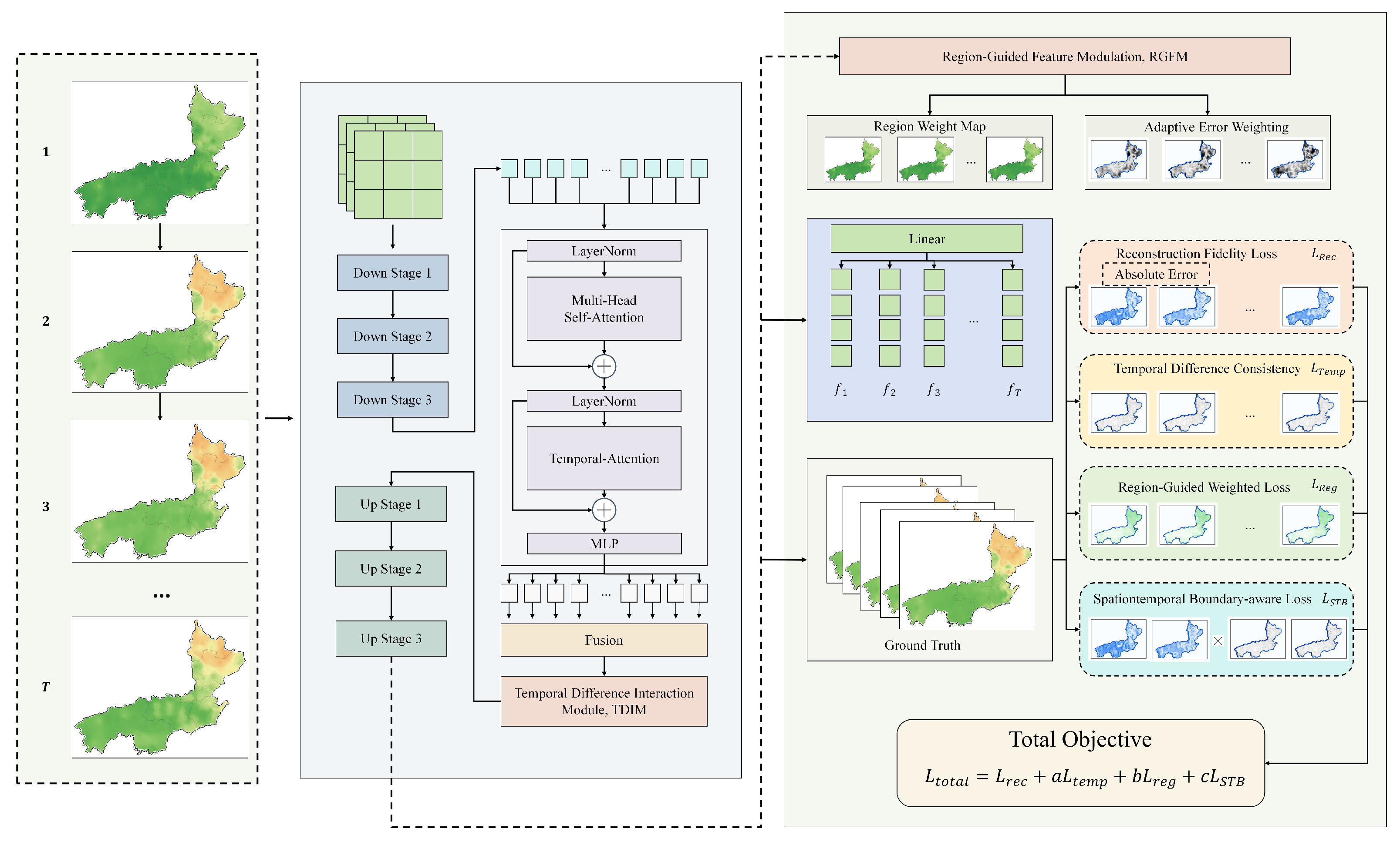
The spatiotemporal prediction of the composite groundwater quality safety index is essentially a regional continuous-field prediction problem. Its objective is not merely to extrapolate the water quality status of individual monitoring sites, but to learn the coupled relationships among the overall spatial pattern, local anomalous regions, and temporal evolution trends from continuous regional groundwater safety state maps. To this end, this study organizes the composite groundwater quality safety index of Yiyang City as a continuous spatial sequence input, enabling the model to perform both regional-scale prediction and community-scale point prediction within a unified framework. Specifically, the input sequence consists of composite groundwater quality safety index maps from multiple historical time steps, where each frame corresponds to the spatial distribution of safety scores at different locations within the study area. The overall model structure is shown in Figure 1. The model first receives the historical regional safety index sequence and extracts multi-scale features ranging from shallow spatial textures to deep regional semantics through a multi-stage encoder. Let the historical input length be T, the prediction horizon be K, and the regional grid size be $H\times W$. The input sequence can be expressed as

$${\mathbf{X}}_{1:T}=\left\{{\mathbf{X}}_1,{\mathbf{X}}_2,\dots ,{\mathbf{X}}_T\right\},{\mathbf{X}}_t\in {\mathbb{R}}^{H\times W\times C},t=1,2,\dots ,T,$$

(1)

where C denotes the number of input channels. When the model directly takes the composite groundwater quality safety index as input, $C=1$; when multi-source environmental variables, historical water quality indicators, or spatial auxiliary factors are further introduced, C can be extended to a multi-channel form. In the encoding stage, a progressive downsampling structure is adopted to compress the spatial resolution and enlarge the receptive field, allowing the model to capture cross-regional water quality correlations. In the decoding stage, spatial details are gradually restored through progressive upsampling, while shallow features are incorporated to preserve regional boundaries, local abrupt changes, and the continuity of spatial distributions.

After obtaining multi-scale spatial features, the model further introduces spatial attention and temporal attention structures to enhance the modeling of regional dependencies and temporal variation patterns. Spatial attention is used to characterize potential associations among different grid regions, while temporal attention is used to identify historical time steps that are more critical for future prediction, thereby improving the model response to pollutant diffusion, short-term temporal fluctuations, and local anomalous changes. This spatiotemporal encoding process can be summarized as

$${\mathbf{Z}}_{1:T}={\mathcal{A}}_{temp}\left({\mathcal{A}}_{spa}\left(\mathcal{E}\left({\mathbf{X}}_{1:T}\right)\right)\right),$$

(2)

where $\mathcal{E}(·)$ denotes the multi-stage spatial encoder, ${\mathcal{A}}_{spa}(·)$ denotes spatial attention modeling, ${\mathcal{A}}_{temp}(·)$ denotes temporal attention modeling, and ${\mathbf{Z}}_{1:T}$ represents the high-level spatiotemporal representation after integrating spatial structures and temporal dynamics. Subsequently, the model integrates encoder and decoder information through a multi-scale feature fusion module, and explicitly models the magnitude and direction of changes in the composite groundwater quality safety index between adjacent time steps using the Temporal Difference Interaction Module. Meanwhile, the Region-Guided Feature Modulation module adaptively adjusts feature responses according to regional weight maps and error-sensitive areas, enabling the model to focus more on spatial units with higher water quality risks or more intense variations. Finally, the model outputs regional prediction maps of the composite groundwater quality safety index for multiple future time steps, and point prediction results for designated communities or monitoring regions can be extracted using a spatial sampling operator. The overall prediction process is formulated as

$$\left({\widehat{\mathbf{Y}}}_{T+1:T+K},{\widehat{\mathbf{y}}}_{p,T+1:T+K}\right)=\left(\mathcal{P}\left({\mathcal{G}}_{reg}\left({\mathcal{F}}_{fuse}\left(\mathcal{D}\left({\mathbf{Z}}_{1:T}\right),{\mathcal{T}}_{diff}\left({\mathbf{Z}}_{1:T}\right)\right)\right)\right),{\mathcal{S}}_p\left({\widehat{\mathbf{Y}}}_{T+1:T+K}\right)\right),$$

(3)

where $\mathcal{D}(·)$ denotes the decoder, ${\mathcal{T}}_{diff}(·)$ denotes the Temporal Difference Interaction Module, ${\mathcal{F}}_{fuse}(·)$ denotes the multi-scale fusion operation, ${\mathcal{G}}_{reg}(·)$ denotes Region-Guided Feature Modulation, $\mathcal{P}(·)$ denotes the prediction head, ${\widehat{\mathbf{Y}}}_{T+1:T+K}$ denotes the regional prediction results for the future K time steps, ${\mathcal{S}}_p(·)$ denotes the spatial sampling or regional aggregation operation corresponding to community location p, and ${\widehat{\mathbf{y}}}_{p,T+1:T+K}$ denotes the point prediction sequence of the designated community. Through the above design, the model can simultaneously account for the overall evolution of regional groundwater quality, small-scale spatial heterogeneity, and dynamic changes in local risk areas, providing a unified modeling basis for groundwater quality prediction, water resource safety zoning, and pollution risk early warning.

3.2. Temporal Difference Interaction Module, TDIM

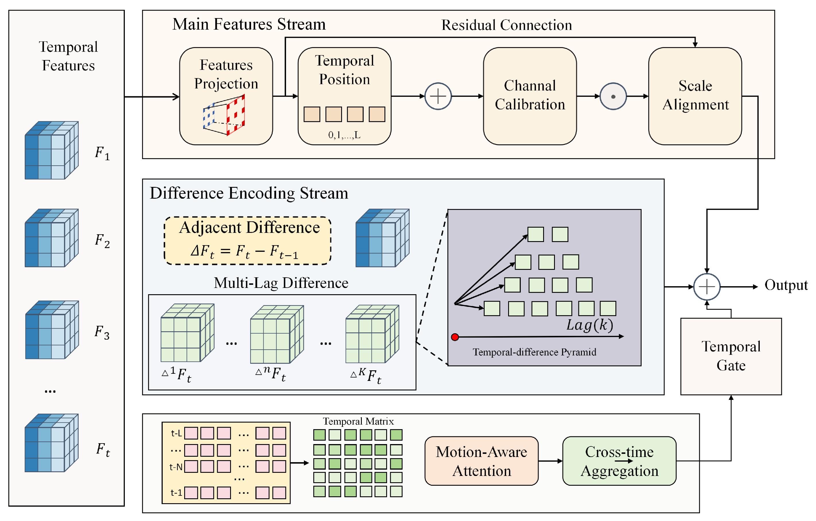
The composite groundwater quality safety index usually exhibits a dynamic process in the temporal dimension, where slow evolution and local abrupt changes coexist. On the one hand, regional water quality status is affected by short-term hydrological variations, groundwater runoff, and gradual changes in pollutant levels, showing continuous variation characteristics. On the other hand, local pollutant inputs, extreme rainfall disturbances, or changes in human activities may lead to abnormal fluctuations within a short period. If only conventional temporal attention or convolutional structures are used, the model may tend to learn the overall trend while showing insufficient response to fine-grained changes between adjacent time steps. To address this issue, this study designs the Temporal Difference Interaction Module (TDIM), which jointly models trend information, differential variations, and cross-temporal dependencies in groundwater quality sequences through the main feature stream, differential encoding stream, and motion-aware temporal aggregation stream. The architecture of the module is shown in Figure 2.

Given the temporal feature sequence from the upstream spatiotemporal encoder, ${\mathbf{F}}_{1:T}=\{{\mathbf{F}}_1,{\mathbf{F}}_2,\dots ,{\mathbf{F}}_T\}$, where ${\mathbf{F}}_t\in {\mathbb{R}}^{H\times W\times C}$, TDIM first performs linear projection on the feature of each time step and introduces learnable temporal positional encoding to preserve temporal order information:

$${\mathbf{U}}_t={\varphi }_p\left({\mathbf{F}}_t\right)+{\mathbf{e}}_t,{\mathbf{e}}_t\in {\mathbb{R}}^{H\times W\times d},t=1,2,\dots ,T,$$

(4)

where ${\varphi }_p(·)$ denotes the feature projection operation, d is the hidden channel dimension, and ${\mathbf{e}}_t$ represents the temporal positional embedding at the t-th time step. This main feature stream is used to preserve the original spatiotemporal semantics and provide a stable basic representation for subsequent differential interaction.

To explicitly characterize the changes in groundwater quality status between adjacent time steps and across multiple temporal intervals, TDIM constructs a differential encoding stream. First, feature differences between adjacent time steps are calculated to capture short-term change direction and change intensity. Then, the operation is further extended to a multi-lag differential form, enabling the model to perceive both short-term fluctuations and accumulated changes across multiple monthly intervals within the input sequence. This process is defined as

$${\Delta }^k{\mathbf{F}}_t={\mathbf{F}}_t-{\mathbf{F}}_{t-k},k\in \mathcal{K},t>k,$$

(5)

where $\mathcal{K}=\{1,2,\dots ,K_d\}$ denotes the set of differential lags. ${\Delta }^1{\mathbf{F}}_t$ corresponds to the adjacent-time-step difference, while larger k values correspond to change responses across wider intervals within the historical input sequence. Furthermore, TDIM organizes the differential features at different lag scales into a temporal difference pyramid and extracts change patterns through a scale-shared encoder:

$${\mathbf{D}}_t={\psi }_d\left(Concat\left[{\Delta }^1{\mathbf{F}}_t,{\Delta }^2{\mathbf{F}}_t,\dots ,{\Delta }^{K_d}{\mathbf{F}}_t\right]\right),$$

(6)

where $Concat[·]$ denotes concatenation along the channel dimension, and ${\psi }_d(·)$ is the differential encoding function. Through this design, the model can not only identify instantaneous changes in the groundwater quality index, but also capture multi-interval temporal processes such as gradual pollutant variation, local diffusion, and short-term water quality recovery.

Based on the differential features, TDIM further introduces motion-aware temporal attention to model the different contributions of historical time steps to the current predicted state. Specifically, the module constructs a temporal correlation matrix according to the current main feature ${\mathbf{U}}_t$ and the historical differential feature ${\mathbf{D}}_i$, and obtains cross-temporal attention weights through normalization:

$${\alpha }_{t,i}={\displaystyle \frac{exp\left(〈{\theta }_q\left({\mathbf{U}}_t\right),{\theta }_k\left({\mathbf{D}}_i\right)〉/\sqrt{d}\right)}{{\sum }_{j=t-L}^{t-1}exp\left(〈{\theta }_q\left({\mathbf{U}}_t\right),{\theta }_k\left({\mathbf{D}}_j\right)〉/\sqrt{d}\right)}},i\in [t-L,t-1],$$

(7)

where L denotes the temporal look-back window, ${\theta }_q(·)$ and ${\theta }_k(·)$ denote the query mapping and key mapping, respectively, and $\langle ·,·\rangle$ denotes the feature similarity measure. Subsequently, the module performs cross-temporal aggregation on historical change features to obtain the motion-aware representation:

$${\mathbf{M}}_t={\displaystyle \sum _{i=t-L}^{t-1}}{\alpha }_{t,i}{\theta }_v\left({\mathbf{D}}_i\right),$$

(8)

where ${\theta }_v(·)$ denotes the value mapping. This aggregation process enables the model to automatically focus on historical change segments that are more informative for explaining the evolution of the current water quality status, thereby alleviating the limitation that a fixed temporal window cannot adapt to different regional change rhythms.

Finally, TDIM performs adaptive fusion between the main feature stream and the differential change stream through channel calibration, scale alignment, and temporal gating mechanisms. Channel calibration is used to enhance feature channels related to water quality changes, scale alignment ensures consistency between main features and differential features in spatial resolution and channel dimension, and temporal gating dynamically controls the fusion ratio between trend information and change information according to the current state. The overall output is expressed as

$${\tilde{\mathbf{F}}}_t={\mathbf{U}}_t+{\gamma }_t\odot \eta \left({\mathbf{D}}_t+{\mathbf{M}}_t\right),{\gamma }_t=\sigma \left(\omega \left[{\mathbf{U}}_t,{\mathbf{D}}_t,{\mathbf{M}}_t\right]\right),$$

(9)

where $\eta (·)$ denotes the scale alignment operation, $\omega (·)$ denotes the gating mapping function, $\sigma (·)$ is the Sigmoid activation function, ⊙ denotes element-wise multiplication, and ${\gamma }_t$ represents the temporal gating weight. Through the above structure, TDIM can preserve the stable spatial pattern of regional groundwater quality while explicitly enhancing adjacent temporal differences, multi-lag variations, and cross-temporal dynamic propagation information, thereby improving the model ability to characterize the spatiotemporal evolution process of the composite groundwater quality safety index.

3.3. Region-Guided Feature Modulation, RGFM

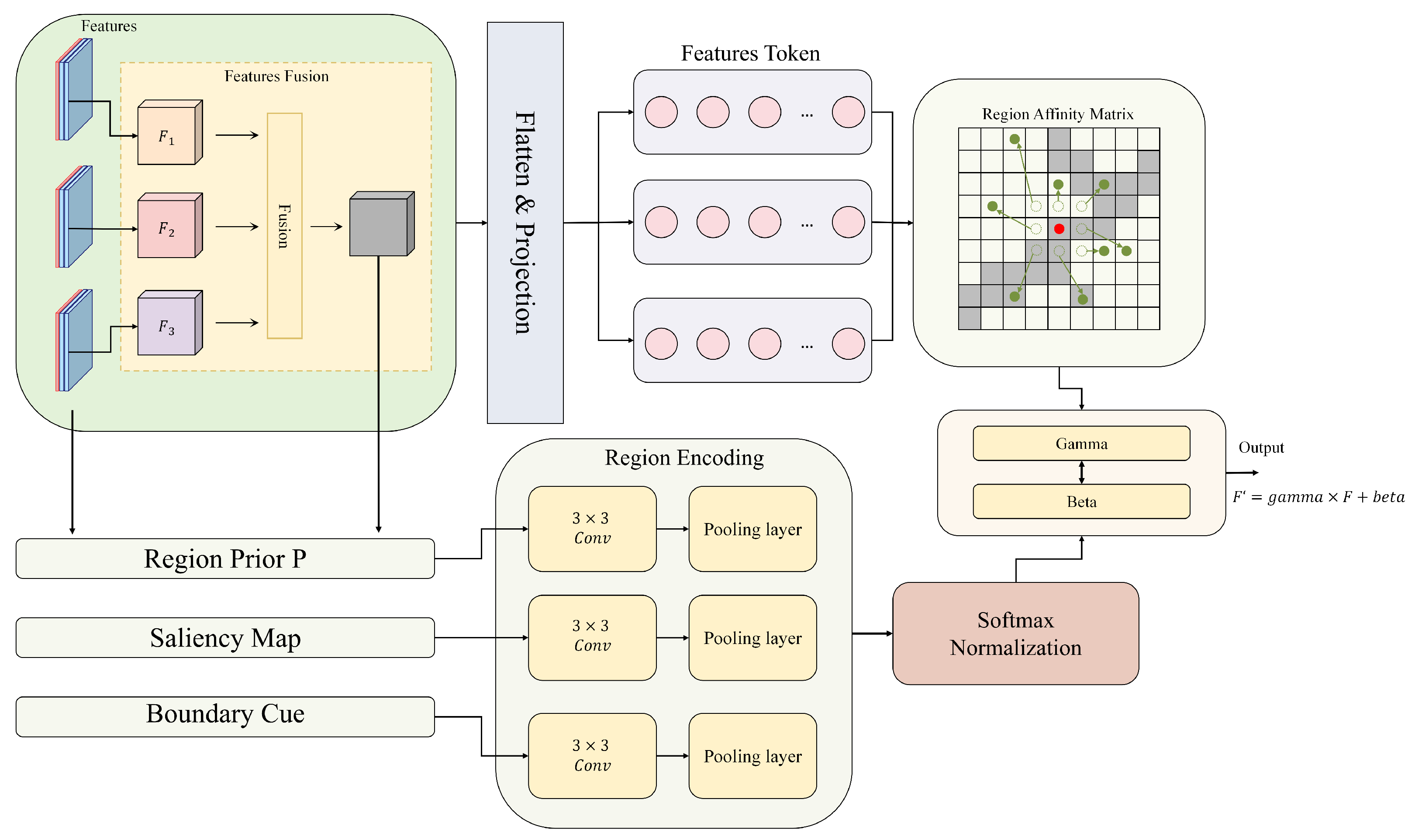
After TDIM enhances temporal differential changes, the model can obtain spatiotemporal features with dynamic-change awareness. However, the spatial distribution of the composite groundwater quality safety index does not change uniformly. Different regions are jointly affected by topographic structures, pollutant inputs, groundwater runoff connectivity, land-use types, and the sparsity of monitoring sites, thus showing evident regional heterogeneity. If the output features of TDIM are directly fed into the prediction head, the model may tend to learn globally smoothed trends while weakening its attention to high-risk regions, spatial boundary regions, and locally significant changing areas. To address this issue, this study designs the Region-Guided Feature Modulation (RGFM) module. Based on spatiotemporal features, RGFM introduces regional priors, saliency responses, and boundary cues, and generates adaptive modulation parameters through regional affinity modeling, thereby enhancing the model ability to represent spatial differences in groundwater quality. The architecture of this module is shown in Figure 3.

Given the features from different scales at the t-th time step, $\{{\tilde{\mathbf{F}}}_t^1,{\tilde{\mathbf{F}}}_t^2,{\tilde{\mathbf{F}}}_t^3\}$, RGFM first performs scale alignment and feature fusion:

$${\mathbf{F}}_t={\varphi }_f\left(Concat\left[{\mathcal{R}}_1\left({\tilde{\mathbf{F}}}_t^1\right),{\mathcal{R}}_2\left({\tilde{\mathbf{F}}}_t^2\right),{\mathcal{R}}_3\left({\tilde{\mathbf{F}}}_t^3\right)\right]\right),$$

(10)

where ${\mathcal{R}}_s(·)$ denotes the spatial alignment operation at the s-th scale, ${\varphi }_f(·)$ denotes the fusion mapping function, and ${\mathbf{F}}_t\in {\mathbb{R}}^{H\times W\times C}$ represents the fused regional spatiotemporal feature. Subsequently, ${\mathbf{F}}_t$ is flattened and projected into regional feature tokens:

$${\mathbf{T}}_t=Proj\left(Flatten\left({\mathbf{F}}_t\right)\right),{\mathbf{T}}_t={\left[{\mathbf{t}}_{t,1},{\mathbf{t}}_{t,2},\dots ,{\mathbf{t}}_{t,N}\right]}^{\top },N=HW.$$

(11)

Here, ${\mathbf{t}}_{t,i}\in {\mathbb{R}}^d$ denotes the feature token of the i-th spatial unit, N is the number of spatial tokens, and d is the token dimension.

To ensure that the regional modulation process relies not only on data-driven features but also on spatial prior knowledge in groundwater quality prediction, RGFM constructs a regional encoding branch. This branch contains three types of inputs: the regional prior map $\mathbf{P}$, the saliency map ${\mathbf{S}}_t$, and the boundary cue map $\mathbf{B}$. Specifically, $\mathbf{P}$ describes relatively stable spatial risk differences within the study area, ${\mathbf{S}}_t$ represents salient response regions in the prediction features at the current time step, and $\mathbf{B}$ is used to characterize administrative boundaries, spatial transition zones, or high-gradient changing regions. These three types of regional cues are encoded by convolution and compressed by pooling to obtain the corresponding regional embeddings:

$${\mathbf{r}}^p=Pool\left({Conv}_{3\times 3}\left(\mathbf{P}\right)\right),{\mathbf{r}}_t^s=Pool\left({Conv}_{3\times 3}\left({\mathbf{S}}_t\right)\right),{\mathbf{r}}^b=Pool\left({Conv}_{3\times 3}\left(\mathbf{B}\right)\right).$$

(12)

On this basis, RGFM performs adaptive normalized fusion on the three types of regional embeddings to obtain a unified region-guided vector:

$${\mathbf{r}}_t=\sum _{q\in \{p,s,b\}}{\lambda }_t^q{\mathbf{r}}_t^q,{\lambda }_t^q={\displaystyle \frac{exp\left({\mathbf{a}}^{\top }{\mathbf{r}}_t^q\right)}{{\sum }_{m\in \{p,s,b\}}exp\left({\mathbf{a}}^{\top }{\mathbf{r}}_t^m\right)}},$$

(13)

where ${\mathbf{r}}_t^p={\mathbf{r}}^p$, ${\mathbf{r}}_t^b={\mathbf{r}}^b$, ${\lambda }_t^q$ denotes the adaptive weight of different regional cues, and $\mathbf{a}$ is a learnable parameter. This design enables the model to dynamically select more important regional constraint information according to the groundwater quality status at the current time step.

After obtaining the regional feature tokens and the region-guided vector, RGFM further constructs a regional affinity matrix to describe the potential relationships among different spatial units. Unlike a fixed adjacency matrix, this affinity matrix simultaneously considers feature similarity, regional prior modulation, and spatial positional relationships, and therefore can more flexibly reflect the non-uniform propagation characteristics of the composite groundwater quality safety index within the region:

$${\mathbf{A}}_{t,ij}={\displaystyle \frac{{\left({\mathbf{W}}_q{\mathbf{t}}_{t,i}\right)}^{\top }\left({\mathbf{W}}_k{\mathbf{t}}_{t,j}\right)}{\sqrt{d}}}+{\mathbf{u}}^{\top }{\psi }_r\left({\mathbf{r}}_t,{\mathbf{p}}_i,{\mathbf{p}}_j\right),$$

(14)

where ${\mathbf{W}}_q$ and ${\mathbf{W}}_k$ denote the query mapping and key mapping, respectively, ${\mathbf{p}}_i$ and ${\mathbf{p}}_j$ denote the positional embeddings of the i-th and j-th spatial units, ${\psi }_r(·)$ denotes the regional relation encoding function, and $\mathbf{u}$ is a learnable vector. Then, Softmax normalization is applied to the regional affinity matrix to obtain the region-guided weight matrix:

$${\mathbf{G}}_{t,ij}={\displaystyle \frac{exp\left({\mathbf{A}}_{t,ij}\right)}{{\sum }_{m=1}^{N}exp\left({\mathbf{A}}_{t,im}\right)}}.$$

(15)

Here, ${\mathbf{G}}_{t,ij}$ represents the regional dependency strength from the i-th spatial unit to the j-th spatial unit, which can be used to selectively aggregate contextual information with similar water quality variation patterns or potential spatial associations.

Based on the region-guided weight matrix, RGFM performs weighted aggregation over all spatial tokens to obtain region-enhanced feature representations. This process enables high-risk regions to obtain supplementary information from regions with similar pollution responses, and allows boundary regions to acquire more stable spatial context from adjacent transition areas, thereby alleviating local prediction discontinuity and blurred regional boundary problems:

$${\overline{\mathbf{t}}}_{t,i}={\displaystyle \sum _{j=1}^N}{\mathbf{G}}_{t,ij}{\mathbf{W}}_v{\mathbf{t}}_{t,j},{\overline{\mathbf{T}}}_t={\left[{\overline{\mathbf{t}}}_{t,1},{\overline{\mathbf{t}}}_{t,2},\dots ,{\overline{\mathbf{t}}}_{t,N}\right]}^{\top }.$$

(16)

Here, ${\mathbf{W}}_v$ denotes the value mapping matrix, and ${\overline{\mathbf{T}}}_t$ is the token sequence enhanced by regional context. Different from directly concatenating regional priors, this aggregation strategy establishes soft connections among spatial units through affinity relationships, enabling the model to automatically learn the propagation and collaborative variation relationships of groundwater quality status within the region.

Finally, RGFM restores the enhanced token sequence into a spatial feature map and generates the scaling parameter ${\gamma }_t$ and shifting parameter ${\beta }_t$ to perform region-guided affine modulation on the original fused feature ${\mathbf{F}}_t$. This modulation mechanism can finely adjust the feature response intensity at different spatial locations without disrupting the backbone spatiotemporal semantics:

$${\gamma }_t,{\beta }_t=Split\left({\varphi }_m\left(Reshape\left({\overline{\mathbf{T}}}_t\right)\right)\right),{\mathbf{F}}_t^{\prime }={\gamma }_t\odot {\mathbf{F}}_t+{\beta }_t+{\mathbf{F}}_t.$$

(17)

Here, ${\varphi }_m(·)$ denotes the modulation parameter generation function, $Split(·)$ denotes splitting the output into the scaling term and shifting term, ⊙ denotes element-wise multiplication, and ${\mathbf{F}}_t^{\prime }$ is the region-modulated feature output by RGFM. Through the above design, RGFM integrates multi-scale spatiotemporal features, regional priors, saliency responses, boundary cues, and regional affinity relationships into a unified modulation framework, enabling the model to focus more sufficiently on key spatial units in groundwater quality prediction and thereby improving the spatial representation ability of both regional-scale prediction and community-scale point prediction.

3.4. Training Objective and Loss Function

The training objective of this study is to enable the model to simultaneously achieve regional reconstruction accuracy, temporal variation consistency, regional risk sensitivity, and spatiotemporal boundary preservation. Given the historical input sequence ${\mathbf{X}}_{1:T}$, the model predicts the composite groundwater quality safety index map for the next month, denoted as ${\widehat{\mathbf{Y}}}_{T+1}$, with the corresponding ground truth denoted as ${\mathbf{Y}}_{T+1}$. In this study, the prediction horizon is fixed to one month, i.e., $K=1$, throughout model training and evaluation. The overall training process is shown in Algorithm 1. In each training batch, the model sequentially performs spatiotemporal feature encoding, TDIM-based temporal difference enhancement, RGFM-based region-guided modulation, and joint optimization with multiple training objectives.

Specifically, the reconstruction fidelity term is used to constrain the overall numerical consistency between the prediction results and the ground truth composite groundwater quality safety index, which is defined as

$${\mathcal{L}}_{rec}={∥{\widehat{\mathbf{Y}}}_{T+1}-{\mathbf{Y}}_{T+1}∥}_1.$$

(18)

Algorithm 1 Training process of the proposed groundwater quality prediction model

Require: Historical groundwater quality sequence ${\mathbf{X}}_{1:T}$, ground truth map ${\mathbf{Y}}_{T+1}$ Ensure: Optimized model parameters $\Theta$ 1: Initialize model parameters $\Theta$ 2: for each training epoch do 3:     for each mini-batch do 4:         Extract multiscale spatiotemporal features from ${\mathbf{X}}_{1:T}$ 5:         Enhance temporal variation features using TDIM 6:         Generate region-guided modulated features using RGFM 7:         Predict the next-month groundwater quality map ${\widehat{\mathbf{Y}}}_{T+1}$ 8:         Compute reconstruction, temporal, region-guided, and STB losses 9:         Update $\Theta$ by back-propagation 10:     end for 11: end for

To enhance the model ability to characterize the temporal variation from the last observed month to the predicted month, this study introduces a one-step temporal variation consistency constraint. Specifically, the predicted and ground-truth temporal changes are first defined as

$$\Delta {\widehat{\mathbf{Y}}}_{T+1}={\widehat{\mathbf{Y}}}_{T+1}-{\mathbf{Y}}_T,\Delta {\mathbf{Y}}_{T+1}={\mathbf{Y}}_{T+1}-{\mathbf{Y}}_T,$$

(19)

where ${\mathbf{Y}}_T$ denotes the integrated groundwater quality risk map of the last observed month in the historical input sequence. The temporal consistency loss jointly constrains the magnitude and direction of the month-to-month variation:

$${\mathcal{L}}_{temp}={∥\left|\Delta {\widehat{\mathbf{Y}}}_{T+1}\right|-\left|\Delta {\mathbf{Y}}_{T+1}\right|∥}_1+\left(1-{\displaystyle \frac{〈\Delta {\widehat{\mathbf{Y}}}_{T+1},\Delta {\mathbf{Y}}_{T+1}〉+ϵ}{{∥\Delta {\widehat{\mathbf{Y}}}_{T+1}∥}_2{∥\Delta {\mathbf{Y}}_{T+1}∥}_2+ϵ}}\right).$$

(20)

The first term constrains the magnitude of groundwater quality variation between two consecutive months, while the second term encourages consistency in the overall direction of temporal change. The inner product and the corresponding norms are computed over the spatial domain.

In addition, the regional weight map ${\mathbf{R}}_{T+1}$ output by RGFM is used to construct a region-guided weighted error, enabling the model to pay more attention to high-risk regions, significantly changing regions, and boundary transition regions:

$${\mathcal{L}}_{reg}={\displaystyle \frac{{∥{\mathbf{R}}_{T+1}\odot \left({\widehat{\mathbf{Y}}}_{T+1}-{\mathbf{Y}}_{T+1}\right)∥}_1}{{∥{\mathbf{R}}_{T+1}∥}_1+ϵ}}.$$

(21)

To further preserve the spatial boundaries of groundwater quality and their temporal variation boundaries, this study designs a spatiotemporal boundary-aware loss, namely STB Loss, which jointly constrains the prediction results through spatial gradients and temporal difference gradients:

$${\mathcal{L}}_{STB}={∥\nabla {\widehat{\mathbf{Y}}}_{T+1}-\nabla {\mathbf{Y}}_{T+1}∥}_1+{∥\nabla \left|\Delta {\widehat{\mathbf{Y}}}_{T+1}\right|-\nabla \left|\Delta {\mathbf{Y}}_{T+1}\right|∥}_1.$$

(22)

Here, the first term preserves the spatial boundary structure of the predicted groundwater quality risk map, while the second term constrains the spatial distribution and boundary structure of the month-to-month variation magnitude. where $\nabla (·)$ denotes the spatial gradient operator, and $ϵ$ is a constant used to prevent division by zero. Finally, the total training objective is formulated as

$${\mathcal{L}}_{total}={\mathcal{L}}_{rec}+\alpha {\mathcal{L}}_{temp}+\beta {\mathcal{L}}_{reg}+\lambda {\mathcal{L}}_{STB},$$

(23)

where $\alpha$, $\beta$, and $\lambda$ denote the weighting coefficients of different loss terms, respectively. Through the above joint optimization, the model can better preserve the temporal continuity, regional risk sensitivity, and spatial boundary structure of the composite groundwater quality safety index while maintaining overall prediction accuracy.

4. Datasets and Evaluation Metrics

4.1. Dataset

Based on groundwater monitoring data from Yiyang City from 2000 to 2023, this study constructs a multi-indicator gridded dataset for spatiotemporal groundwater quality prediction and water environmental safety assessment. The raw data consist of monthly water quality observations from groundwater monitoring sites within the study area. Each record contains the longitude and latitude of the monitoring site, monitoring time, and multiple groundwater quality indicators. To ensure spatial consistency, the administrative boundary file of Yiyang City is first used to spatially filter the monitoring sites, and only valid groundwater monitoring samples located inside or on the boundary of the study area are retained. The resulting rectangular raster grid has a fixed spatial size of $512\times 512$ cells, of which approximately $67.3\%$ fall outside the administrative boundary of Yiyang City and are treated as invalid spatial locations. Considering that groundwater quality is jointly affected by multiple hydrochemical factors, this study selects dissolved oxygen, total nitrogen, electrical conductivity, dissolved organic carbon, pH, permanganate index, and total phosphorus as the main evaluation indicators. These indicators characterize groundwater quality from the perspectives of redox conditions, nitrogen and phosphorus nutrient accumulation, ionic content, organic pollution load, and acid–base status. The meaning, risk direction, and normalization strategy of each indicator are shown in

Table 1. Water quality indicators used for constructing the integrated groundwater quality risk index.

Indicator	Symbol	Indicator Type	Risk Direction	Environmental Meaning
Dissolved oxygen	DO	Benefit-type	Lower value, higher risk	Indicates groundwater oxygen condition and self-purification capacity.
Total nitrogen	TN	Cost-type	Higher value, higher risk	Indicates nitrogen enrichment and potential nutrient pollution.
Electrical conductivity	EC	Cost-type	Higher value, higher risk	Reflects dissolved ions, salinity, and mineralization level.
Dissolved organic carbon	DOC	Cost-type	Higher value, higher risk	Represents soluble organic matter and organic pollution load.
pH	pH	Optimum-type	Larger deviation, higher risk	Describes groundwater acid–base balance and chemical stability.
Permanganate index	CODMn	Cost-type	Higher value, higher risk	Reflects reducing substances and organic pollution pressure.
Total phosphorus	TP	Cost-type	Higher value, higher risk	Indicates phosphorus enrichment and potential pollution risk.

.

Since different groundwater quality indicators have obvious differences in units, value ranges, and risk directions, this study first maps all indicators into a unified $[0,1]$ risk space. Let $x_{i,t}^m$ denote the observed value of the m-th indicator at the i-th groundwater monitoring site at time t, and let $q_1^m$ and $q_{99}^m$ denote the 1st and 99th percentiles of this indicator calculated exclusively from the training period, respectively. The percentile statistics obtained from the training period were fixed and directly applied to the validation and test periods without recalculation. For cost-type indicators, including total nitrogen, electrical conductivity, dissolved organic carbon, permanganate index, and total phosphorus, higher values indicate greater groundwater quality risk. The normalized risk value is defined as

$$r_{i,t}^m=\mathrm{clip}\left({\displaystyle \frac{x_{i,t}^m-q_1^m}{q_{99}^m-q_1^m}},0,1\right).$$

(24)

For benefit-type indicators such as dissolved oxygen, higher values usually indicate better groundwater environmental conditions. Therefore, reverse normalization is adopted:

$$r_{i,t}^m=\mathrm{clip}\left({\displaystyle \frac{q_{99}^m-x_{i,t}^m}{q_{99}^m-q_1^m}},0,1\right).$$

(25)

For indicators with a suitable range, such as pH, this study takes $7.5$ as the reference suitable center and constructs the risk value according to its deviation:

$$r_{i,t}^m=\mathrm{clip}\left({\displaystyle \frac{|x_{i,t}^m-7.5|}{1.5}},0,1\right).$$

(26)

On this basis, the risk values of multiple valid indicators at the same groundwater monitoring site are averaged to obtain the integrated groundwater quality risk index:

$$R_{i,t}={\displaystyle \frac{1}{M_{i,t}}}{\displaystyle \sum _{m=1}^{M_{i,t}}}{r}_{i,t}^m,$$

(27)

where $M_{i,t}$ denotes the number of indicators with valid observations at the i-th monitoring site at time t. The value range of $R_{i,t}$ is $[0,1]$, and a larger value indicates a higher integrated groundwater quality risk. In this way, dissolved oxygen, total nitrogen, electrical conductivity, dissolved organic carbon, pH, permanganate index, and total phosphorus are uniformly transformed into an integrated evaluation target with consistent risk semantics, thereby avoiding scale bias caused by directly modeling indicators with different units and different risk directions.

After obtaining the integrated groundwater quality risk index at the monitoring-site scale, this study further converts the discrete monitoring data into continuous regional grid sequences. Specifically, a spatial mask is generated based on the administrative boundary of Yiyang City, and a regular longitude–latitude grid is constructed at a spatial resolution of $0.01°$. For each month, inverse distance weighting interpolation is used to map the risk values of groundwater monitoring sites to grid cells within the study area. Let s denote the grid location to be estimated, and let ${\mathcal{N}}_k\left(s\right)$ denote the set of its neighboring monitoring sites. The integrated groundwater quality risk value at this location is expressed as

$${\widehat{R}}_t\left(s\right)={\displaystyle \frac{{\sum }_{j\in {\mathcal{N}}_k\left(s\right)}{w}_j\left(s\right)R_{j,t}}{{\sum }_{j\in {\mathcal{N}}_k\left(s\right)}{w}_j\left(s\right)}},w_j\left(s\right)={\displaystyle \frac{1}{{\left(d(s,s_j)+ϵ\right)}^p}},$$

(28)

where $d(s,s_j)$ denotes the spatial distance between the grid location s and the j-th groundwater monitoring site, $k=12$ denotes the number of neighboring monitoring sites, $p=2$ denotes the distance decay coefficient, and $ϵ$ is a very small constant used to avoid division by zero. Subsequently, missing grid cells inside the boundary are filled using nearest-neighbor completion and smoothing to generate continuous and stable monthly groundwater quality risk maps. Finally, the gridded results of all months are organized as a spatiotemporal tensor ${\mathbf{X}}_{1:T}\in {\mathbb{R}}^{T\times H\times W\times C}$, where the channel dimension includes the integrated groundwater quality risk index and the risk maps of individual indicators. The model uses the regional grid sequence of the previous consecutive 6 months as input to predict the integrated groundwater quality risk distribution of the next month:

$${\mathbf{X}}_{t-5:t}⟶{\mathbf{Y}}_{t+1}.$$

(29)

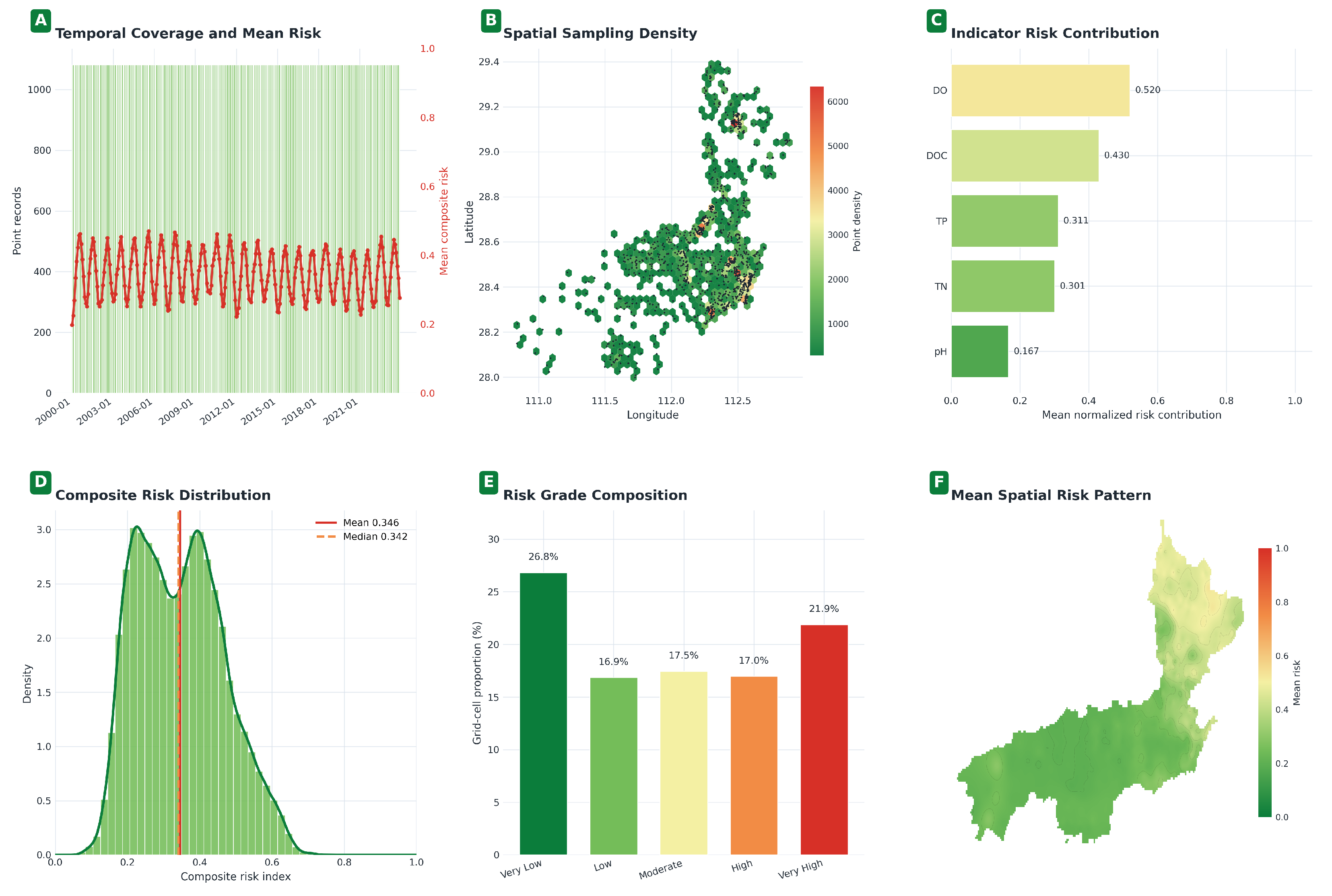
In addition, this study further divides groundwater quality risk levels according to the quantile thresholds of the integrated risk index, which are used for regional water quality safety zoning and visualization of prediction results. This data construction strategy transforms discrete groundwater monitoring observations into a regional spatiotemporal prediction dataset with clear spatial boundaries, continuous temporal structure, and unified risk semantics, providing a data foundation for groundwater quality evolution modeling and water environmental safety assessment. Finally, the overall statistics and examples of the dataset are given, as shown in Figure 4.

4.2. Evaluation Metric

To comprehensively evaluate the predictive performance of the model for integrated groundwater quality risk maps, this study adopts the Structural Similarity Index Measure, Peak Signal-to-Noise Ratio, Mean Absolute Error, and Root Mean Square Error as evaluation metrics. Let the ground-truth groundwater quality risk map be denoted as $\mathbf{Y}$, and the model prediction be denoted as $\widehat{\mathbf{Y}}$. There are N valid grid cells in the image, and ${\mathbf{Y}}_i$ and ${\widehat{\mathbf{Y}}}_i$ denote the ground-truth value and predicted value of the i-th grid cell, respectively. Since the prediction target in this study is the normalized integrated groundwater quality risk index, whose value range is $[0,1]$, all related metrics are calculated under a unified numerical scale.

The Structural Similarity Index Measure (SSIM) is used to measure the consistency between the predicted risk map and the ground-truth risk map in terms of luminance, contrast, and structural distribution. Unlike simple pixel-level errors, SSIM focuses more on whether the overall spatial structure is correctly preserved. Therefore, it is suitable for evaluating the model’s ability to predict the spatial distribution pattern, regional boundaries, and local variation characteristics of groundwater quality risk. The closer the SSIM value is to 1, the more similar the predicted result is to the ground truth in terms of spatial structure. It is defined as

$$\mathrm{SSIM}={\displaystyle \frac{(2{\mu }_{\mathbf{Y}}{\mu }_{\widehat{\mathbf{Y}}}+C_1)(2{\sigma }_{\mathbf{Y}\widehat{\mathbf{Y}}}+C_2)}{({\mu }_{\mathbf{Y}}^2+{\mu }_{\widehat{\mathbf{Y}}}^2+C_1)({\sigma }_{\mathbf{Y}}^2+{\sigma }_{\widehat{\mathbf{Y}}}^2+C_2)}},$$

(30)

where ${\mu }_{\mathbf{Y}}$ and ${\mu }_{\widehat{\mathbf{Y}}}$ denote the mean values of the ground-truth map and the predicted map, respectively; ${\sigma }_{\mathbf{Y}}^2$ and ${\sigma }_{\widehat{\mathbf{Y}}}^2$ denote their variances; ${\sigma }_{\mathbf{Y}\widehat{\mathbf{Y}}}$ denotes the covariance between them; and $C_1$ and $C_2$ are stability constants used to avoid division by zero.

The Peak Signal-to-Noise Ratio (PSNR) is used to evaluate the overall reconstruction quality of the predicted result relative to the ground truth. PSNR is calculated based on the mean squared error and can reflect the noise level and numerical reconstruction error in the predicted risk map. For the groundwater quality risk prediction task, a higher PSNR indicates that the model can more accurately recover the overall numerical distribution of the regional risk map and reduce spatial noise caused by prediction errors. It is defined as

$$\mathrm{PSNR}=10{log}_{10}\left({\displaystyle \frac{L^2}{\frac{1}{N}{\sum }_{i=1}^N{\left({\mathbf{Y}}_i-{\widehat{\mathbf{Y}}}_i\right)}^2}}\right),$$

(31)

where L denotes the maximum possible value of the risk index. Since the integrated groundwater quality risk index in this study is normalized to $[0,1]$, L is set to 1. A larger PSNR value indicates a smaller reconstruction error between the predicted result and the ground truth.

The Mean Absolute Error (MAE) is used to measure the average absolute deviation between predicted values and ground-truth values. This metric has intuitive physical meaning and can directly reflect the average prediction error of the model at each valid grid cell. For groundwater quality risk prediction, a lower MAE indicates that the model can more accurately estimate the integrated risk level at different spatial locations and reduce the average bias in regional risk assessment. MAE is defined as

$$\mathrm{MAE}={\displaystyle \frac{1}{N}}{\displaystyle \sum _{i=1}^N}\left|{\mathbf{Y}}_i-{\widehat{\mathbf{Y}}}_i\right|.$$

(32)

Here, N denotes the number of valid grid cells within the boundary of the study area. A smaller MAE value indicates that the model prediction is closer to the true groundwater quality risk distribution.

The Root Mean Square Error (RMSE) is used to measure the square root of the mean squared error between predicted values and ground-truth values. Compared with MAE, RMSE is more sensitive to larger prediction deviations, and therefore can more prominently reflect prediction errors in high-risk areas, abrupt-change areas, or local abnormal regions. For the spatiotemporal groundwater quality prediction task, a lower RMSE indicates that the model can not only maintain overall prediction accuracy but also effectively reduce large local errors. RMSE is defined as

$$\mathrm{RMSE}=\sqrt{{\displaystyle \frac{1}{N}}{\sum }_{i=1}^N{\left({\mathbf{Y}}_i-{\widehat{\mathbf{Y}}}_i\right)}^2}.$$

(33)

A smaller RMSE value indicates that both the overall error and local large errors of the model in regional groundwater quality risk prediction are lower.

5. Experimental Results and Analysis

5.1. Experimental Setup

The experiments in this study were conducted on an NVIDIA H100 GPU computing platform, and both model training and testing were implemented based on the PyTorch 2.1 deep learning framework. To ensure the reproducibility of the experimental results, all input data were uniformly processed according to the aforementioned data construction procedure. Specifically, the groundwater monitoring data of Yiyang City were first mapped into monthly regular grid sequences. Then, the multi-channel groundwater quality risk maps of the previous consecutive 6 months were used as historical inputs to predict the integrated groundwater quality risk map of the next month. The monthly sequences were divided chronologically into training, validation, and test sets at a ratio of 7:1:2 according to their original temporal order, with the earliest 70% used for training, the subsequent 10% used for validation, and the latest 20% used for testing. No random shuffling was performed across the monthly grids. In addition, the six-month input windows were constructed independently within each subset and were not allowed to cross the boundaries between the training, validation, and test periods, thereby avoiding temporal overlap across different data subsets. During model training, the AdamW optimizer was adopted for parameter updating, and reconstruction constraints related to mean squared error, temporal difference consistency constraints, region-guided constraints, and spatiotemporal boundary preservation constraints were jointly optimized. In the ablation experiments, SimVPv1 was adopted as the Baseline, and TDIM, RGFM, and STB Loss were introduced on top of this baseline to evaluate their individual and combined contributions. The main experimental environment, data processing parameters, and training hyperparameters are shown in

Table 2. Experimental environment and hyperparameter settings.

Setting	Value
Prediction target	Integrated groundwater quality risk index
Grid resolution	$0.01°$
Spatial interpolation method	Inverse distance weighting interpolation
Number of neighboring points	$k=12$
Distance decay coefficient	$p=2$
Historical input length	6 months
Deep learning framework	PyTorch
GPU device	NVIDIA H100
Optimizer	AdamW
Initial learning rate	$1\times {10}^{-4}$
Weight decay	$1\times {10}^{-5}$
Prediction horizon	1 month ($K=1$)
Batch size	8
Training epochs	200

.

5.2. Comparison of Experimental Results with Other Models

To verify the effectiveness of the proposed method in the spatiotemporal groundwater quality prediction task, this section compares the proposed model with several representative prediction models. All models use the same data split, input sequence length, prediction horizon, and evaluation metrics to ensure the fairness of the experimental comparison. By uniformly evaluating the performance of different models in terms of SSIM, PSNR, MAE, and RMSE, the comprehensive performance of the proposed method can be further analyzed in terms of spatial structure preservation, numerical reconstruction accuracy, and regional risk prediction stability. The experimental results are shown in

Table 3. Comparison results of different models for groundwater quality spatiotemporal prediction. The results are reported as mean ± standard deviation over three random seeds, and the best results are highlighted in bold.

Method	SSIM ↑	PSNR ↑	MAE ↓	RMSE ↓
3DCNN [29]	$0.9278\pm 0.0161$	$31.91\pm 1.46$	$1.07\times {10}^{-2}\pm 1.78\times {10}^{-3}$	$2.54\times {10}^{-2}\pm 3.19\times {10}^{-3}$
PredRNN [30]	$0.9099\pm 0.0109$	$33.49\pm 1.33$	$1.30\times {10}^{-2}\pm 1.35\times {10}^{-3}$	$2.12\times {10}^{-2}\pm 4.77\times {10}^{-3}$
SwinLSTM [31]	$0.9397\pm 0.0178$	$34.68\pm 1.66$	$1.12\times {10}^{-2}\pm 2.07\times {10}^{-3}$	$1.85\times {10}^{-2}\pm 6.30\times {10}^{-3}$
UniST [32]	$0.9370\pm 0.0079$	$35.85\pm 1.54$	$1.07\times {10}^{-2}\pm 2.52\times {10}^{-3}$	$1.67\times {10}^{-2}\pm 2.74\times {10}^{-3}$
MLPST [33]	$0.9366\pm 0.0127$	$38.57\pm 1.41$	$1.01\times {10}^{-2}\pm 7.55\times {10}^{-4}$	$1.18\times {10}^{-2}\pm 5.77\times {10}^{-3}$
MGSFformer [34]	$0.9104\pm 0.0091$	$31.78\pm 1.66$	$1.34\times {10}^{-2}\pm 2.02\times {10}^{-3}$	$2.58\times {10}^{-2}\pm 5.67\times {10}^{-3}$
SimVPv2 [35]	$0.9196\pm 0.0051$	$32.10\pm 1.21$	$1.18\times {10}^{-2}\pm 1.61\times {10}^{-3}$	$2.48\times {10}^{-2}\pm 5.16\times {10}^{-3}$
VMRNN [36]	$0.9604\pm 0.0074$	$37.57\pm 2.28$	$8.78\times {10}^{-3}\pm 3.15\times {10}^{-3}$	$1.32\times {10}^{-2}\pm 5.00\times {10}^{-3}$
OpenSTL [37]	$0.9271\pm 0.0160$	$34.46\pm 0.94$	$9.79\times {10}^{-3}\pm 2.63\times {10}^{-3}$	$1.89\times {10}^{-2}\pm 3.81\times {10}^{-3}$
STRPM [38]	$0.9238\pm 0.0094$	$34.81\pm 1.83$	$8.09\times {10}^{-3}\pm 1.14\times {10}^{-3}$	$1.82\times {10}^{-2}\pm 3.20\times {10}^{-3}$
UniFlow [39]	$0.9357\pm 0.0138$	$33.89\pm 2.18$	$8.67\times {10}^{-3}\pm 1.83\times {10}^{-3}$	$2.02\times {10}^{-2}\pm 3.39\times {10}^{-3}$
TSF-mLSTM [40]	$0.9216\pm 0.0124$	$33.59\pm 2.31$	$1.42\times {10}^{-2}\pm 2.88\times {10}^{-3}$	$2.09\times {10}^{-2}\pm 5.53\times {10}^{-3}$
AMV-STECNet [41]	$0.9528\pm 0.0095$	$35.79\pm 1.86$	$8.09\times {10}^{-3}\pm 2.59\times {10}^{-3}$	$1.62\times {10}^{-2}\pm 3.85\times {10}^{-3}$
Ours	$\mathbf{0}.\mathbf{9814}\pm \mathbf{0}.\mathbf{0085}$	$\mathbf{40}.\mathbf{47}\pm \mathbf{2}.\mathbf{19}$	$\mathbf{2}.\mathbf{80}\times {\mathbf{10}}^{-\mathbf{3}}\pm \mathbf{1}.\mathbf{50}\times {\mathbf{10}}^{-\mathbf{3}}$	$\mathbf{9}.\mathbf{70}\times {\mathbf{10}}^{-\mathbf{3}}\pm \mathbf{2}.\mathbf{69}\times {\mathbf{10}}^{-\mathbf{3}}$

.

As shown in Table 3, the proposed method achieves the best results on all four metrics, including SSIM, PSNR, MAE, and RMSE, indicating that the proposed model has stronger comprehensive prediction capability for the spatiotemporal groundwater quality prediction task. Specifically, the SSIM of the proposed method reaches $0.9814$, which is higher than $0.9604$ of VMRNN and $0.9528$ of AMV-STECNet. This indicates that the proposed model can better preserve the spatial structure, regional morphology, and boundary continuity of groundwater quality risk maps. In terms of reconstruction quality, the PSNR of the proposed method reaches $40.47$, which is clearly superior to those of the other comparison models, suggesting that the overall numerical deviation between the predicted results and the ground-truth risk maps is smaller. For the error metrics, the MAE and RMSE of the proposed method are $2.80\times {10}^{-3}$ and $9.70\times {10}^{-3}$, respectively, both of which are lower than those of all baseline models. This demonstrates that the proposed model can not only reduce the average prediction error but also effectively suppress large local deviations.

The superior performance of the proposed method mainly benefits from its dedicated design for the evolution characteristics of groundwater quality. TDIM explicitly models short-term fluctuations, cumulative changes, and cross-time dynamic propagation relationships of groundwater quality risk through adjacent temporal differences, multi-lag temporal differences, and temporal gating mechanisms, thereby improving the model’s ability to capture monthly variation trends. RGFM further combines regional priors, salient responses, and boundary information to adaptively modulate features in different spatial regions, enabling the model to focus more on high-risk regions, spatial transition zones, and local abnormal variation areas. Meanwhile, STB Loss constrains the prediction results from both spatial gradients and temporal difference gradients, which helps preserve the boundary structure of risk maps and the consistency of temporal variations. Therefore, compared with comparison methods that rely only on convolution, recurrent modeling, or general spatiotemporal prediction structures, the proposed model can more sufficiently learn the spatial heterogeneity and temporal evolution patterns of groundwater quality risk.

5.3. Ablation Test Results

To further verify the contribution of each key component in the proposed model to the spatiotemporal prediction performance of groundwater quality, this section designs ablation experiments by individually introducing TDIM, RGFM, and STB Loss into the baseline model. The experimental results are shown in

Table 4. Ablation results of the proposed modules and loss function. The results are reported as mean ± standard deviation over three different random seeds, and the best results are highlighted in bold.

Method	SSIM ↑	PSNR ↑	MAE ↓	RMSE ↓
Baseline	$0.9195\pm 0.0151$	$35.01\pm 1.21$	$1.01\times {10}^{-2}\pm 1.60\times {10}^{-3}$	$1.79\times {10}^{-2}\pm 2.40\times {10}^{-3}$
Baseline + TDIM	$0.9342\pm 0.0137$	$37.41\pm 1.23$	$7.95\times {10}^{-3}\pm 1.89\times {10}^{-3}$	$1.49\times {10}^{-2}\pm 2.10\times {10}^{-3}$
Baseline + RGFM	$0.9531\pm 0.0104$	$38.13\pm 1.90$	$6.16\times {10}^{-3}\pm 1.57\times {10}^{-3}$	$1.33\times {10}^{-2}\pm 2.18\times {10}^{-3}$
Baseline + STB Loss	$0.9593\pm 0.0116$	$38.28\pm 1.06$	$4.64\times {10}^{-3}\pm 1.63\times {10}^{-3}$	$1.24\times {10}^{-2}\pm 2.23\times {10}^{-3}$
Ours	$\mathbf{0}.\mathbf{9814}\pm \mathbf{0}.\mathbf{0085}$	$\mathbf{40}.\mathbf{47}\pm \mathbf{2}.\mathbf{19}$	$\mathbf{2}.\mathbf{80}\times {\mathbf{10}}^{-\mathbf{3}}\pm \mathbf{1}.\mathbf{50}\times {\mathbf{10}}^{-\mathbf{3}}$	$\mathbf{9}.\mathbf{70}\times {\mathbf{10}}^{-\mathbf{3}}\pm \mathbf{2}.\mathbf{69}\times {\mathbf{10}}^{-\mathbf{3}}$

. All ablation variants are evaluated under the same data split, training strategy, and evaluation metrics to ensure comparability. By comparing each single-component variant with the baseline and the complete model, the roles of temporal difference modeling, region-guided feature modulation, and spatiotemporal boundary constraints can be more clearly assessed.

As shown in Table 4, individually introducing TDIM, RGFM, or STB Loss improves the prediction performance compared with the Baseline, indicating that each component contributes positively to groundwater quality risk prediction. The TDIM variant improves PSNR and reduces MAE and RMSE, suggesting that temporal difference interaction helps the model capture adjacent-month variations and cumulative evolution trends. The RGFM variant achieves clear gains in SSIM and error-related metrics, showing that region-guided modulation strengthens the representation of spatial heterogeneity and regional correlations. The STB Loss variant further reduces prediction errors, indicating that spatiotemporal boundary constraints help preserve local transition regions and abrupt-change areas. The complete model achieves the best results across all metrics, demonstrating that TDIM, RGFM, and STB Loss provide complementary improvements when jointly integrated.

5.4. Experimental Results of Loss Function Varying with Epoch

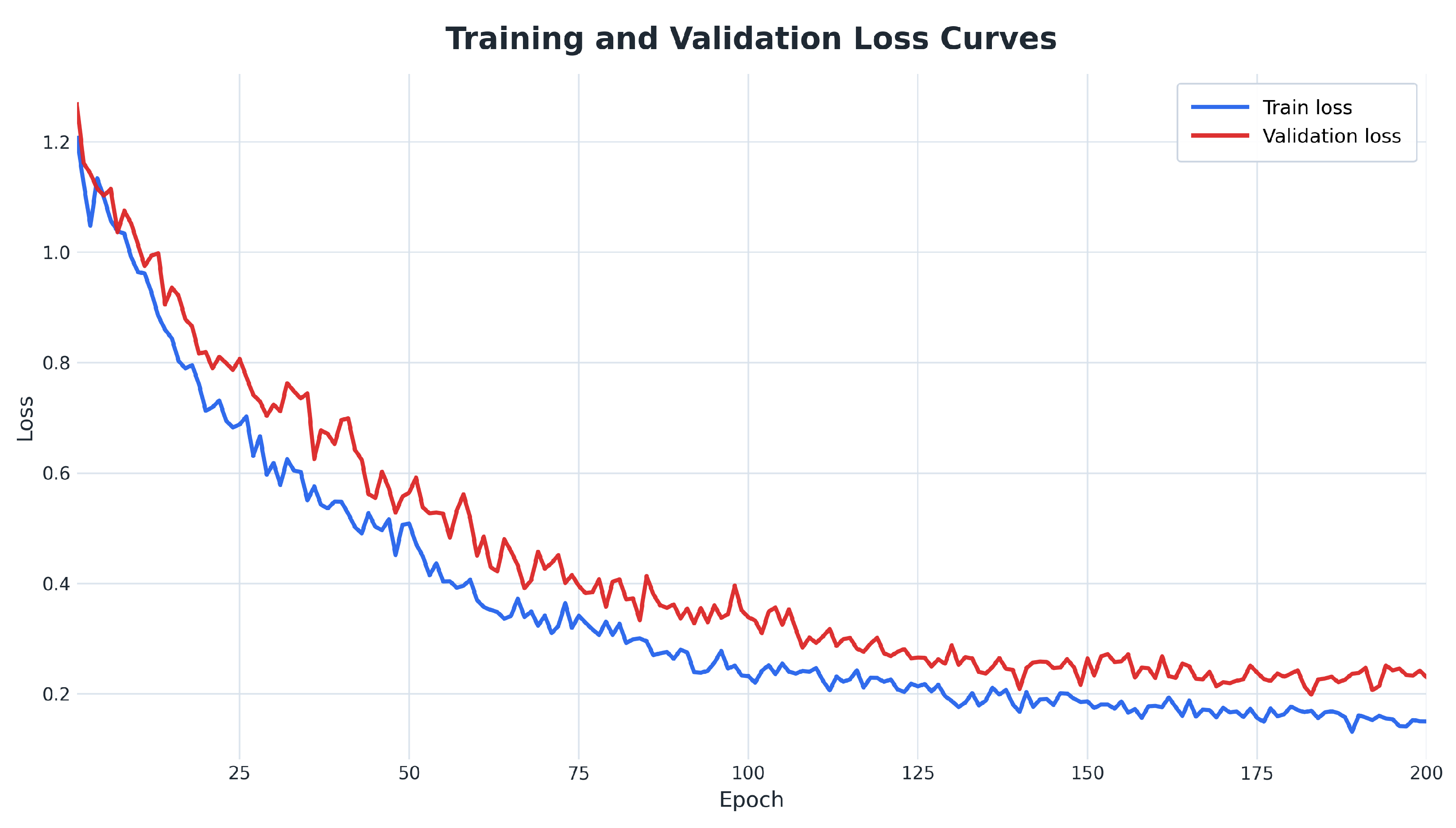
To analyze the convergence and optimization stability of the model training process, this study further plots the loss curves of the training set and validation set with respect to training epochs. This experiment can reflect the model’s fitting ability for groundwater quality risk distributions during the iterative optimization process, and can also be used to observe whether there are obvious oscillations, underfitting, or overfitting during training. The changing trends of training loss and validation loss are shown in Figure 5.

Both the training loss and validation loss decrease rapidly in the early stage, indicating that the model can learn the main spatial distribution characteristics and temporal evolution patterns in groundwater quality risk maps within a relatively short training period. As the number of training epochs increases, the decreasing rates of the two curves gradually slow down and tend to become stable in the later stage, suggesting that the parameter optimization process of the model gradually converges. The validation loss is generally higher than the training loss but maintains a consistent downward trend, and there is no continuous enlargement or abnormal separation between the two curves. This indicates that the model’s fitting on the training data does not significantly sacrifice its generalization ability on the validation set. In the later stage, the validation loss shows slight fluctuations, which may be related to local high-risk areas, uneven distribution of monitoring sites, and uncertainty in monthly-scale variations in the spatiotemporal groundwater quality data. However, the overall trend remains stable, demonstrating that the proposed model has good training stability and generalization performance.

5.5. Visualization Comparison with Competitive Models

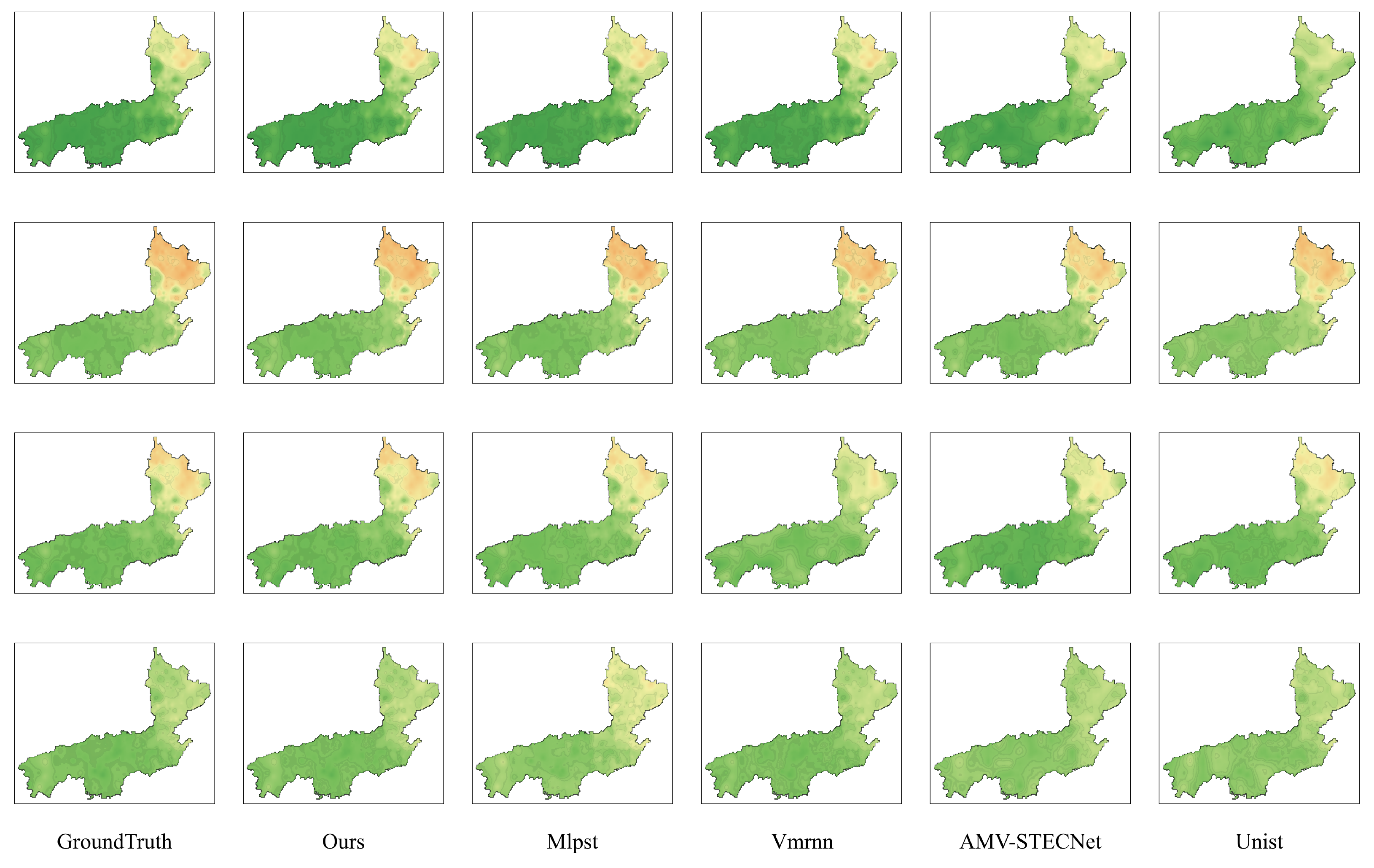
To further analyze the prediction differences among different models from the perspective of spatial distribution, this study selects several representative suboptimal models with relatively close performance in the quantitative experiments for visual comparison, including MLPST, VMRNN, AMV-STECNet, and UniST. These models are selected because they outperform most baseline methods in the aforementioned comparison experiments and can serve as more competitive reference models, thereby providing a stricter evaluation of the advantages of the proposed method in spatial prediction of groundwater quality risk. The groundwater quality risk prediction results of different models on different temporal samples are shown in Figure 6.

As shown in Figure 6, different models can generally recover the overall spatial pattern of groundwater quality risk in the study area, but clear differences remain in local risk intensity, transition-region continuity, and high-risk region characterization. The prediction results of MLPST and UniST are generally smooth and can preserve the basic contours of large-scale low-risk regions, but they tend to weaken details in local high-risk patches and spatial gradient transition areas. VMRNN shows relatively strong responses to certain spatial variations, but obvious local texture fluctuations can be observed in its prediction maps, indicating that recurrent temporal modeling may introduce certain spatial instability when handling continuous regional risk fields. AMV-STECNet can capture the main risk regions relatively well, but risk intensity deviations still exist in some boundary transition areas. In contrast, the prediction maps generated by the proposed method are more consistent with the Ground Truth in terms of overall color distribution, the morphology of northern high-risk regions, and the continuity of central and southern low-risk regions. This indicates that the proposed model can not only predict the numerical level of groundwater quality risk, but also more stably preserve regional spatial structures and local risk differences.

5.6. Residual Visualization Analysis

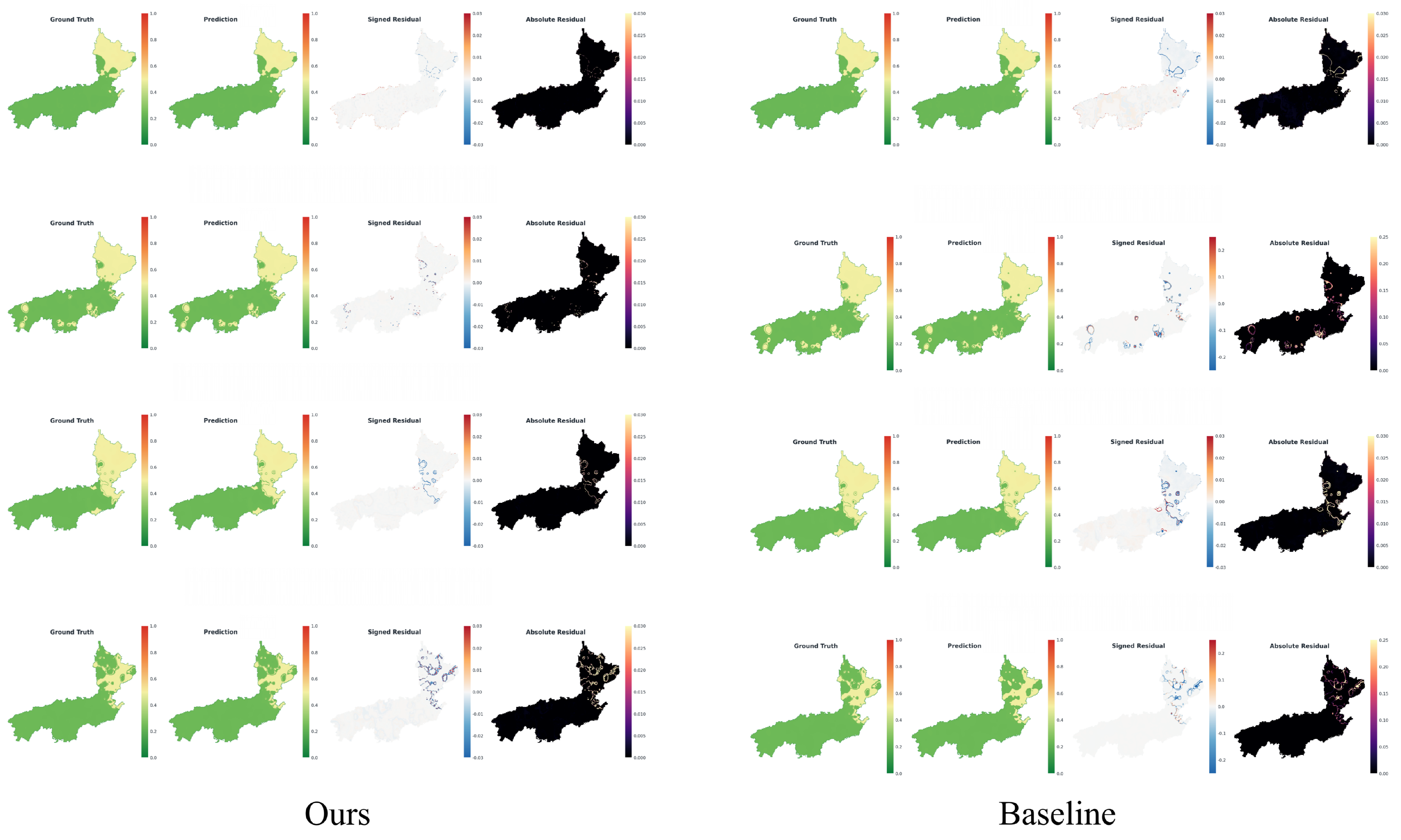
After completing the comparison of overall prediction performance, this section further analyzes the prediction reliability of the model from the perspective of spatial error distribution. Since some models in the aforementioned comparison experiments have already shown suboptimal performance except for the proposed method, the visualization analysis mainly selects the proposed model and the baseline model as references, so as to observe the differences in error distribution among different methods in local risk regions, boundary transition regions, and abnormal variation regions. In this study, the ground-truth map, predicted map, signed residual map, and absolute residual map are jointly displayed to more intuitively evaluate the error sources of the model in spatial reconstruction of groundwater quality risk.

Residual maps can provide more fine-grained error localization information than overall prediction maps. As shown in Figure 7, the prediction results of the proposed method maintain high consistency with the ground-truth risk maps in the main spatial distribution, and the signed residuals are mainly concentrated around zero, indicating that the model does not show obvious systematic overestimation or underestimation. In contrast, the Baseline shows more obvious alternating positive and negative residuals in some local patches, risk boundaries, and high-gradient regions, suggesting that it has insufficient ability to characterize the spatial transition relationships of groundwater quality risk variations. The absolute residual maps further show that the errors of the proposed method are mainly scattered and that the high-error regions cover a relatively small area, whereas the errors of the Baseline are more likely to aggregate along risk boundaries or local abnormal regions. This phenomenon indicates that the proposed model not only improves the overall numerical prediction accuracy, but also more effectively suppresses the diffusion of local errors, making the prediction results more stable in terms of spatial continuity and risk boundary preservation.

5.7. Paired Bootstrap Significance Analysis

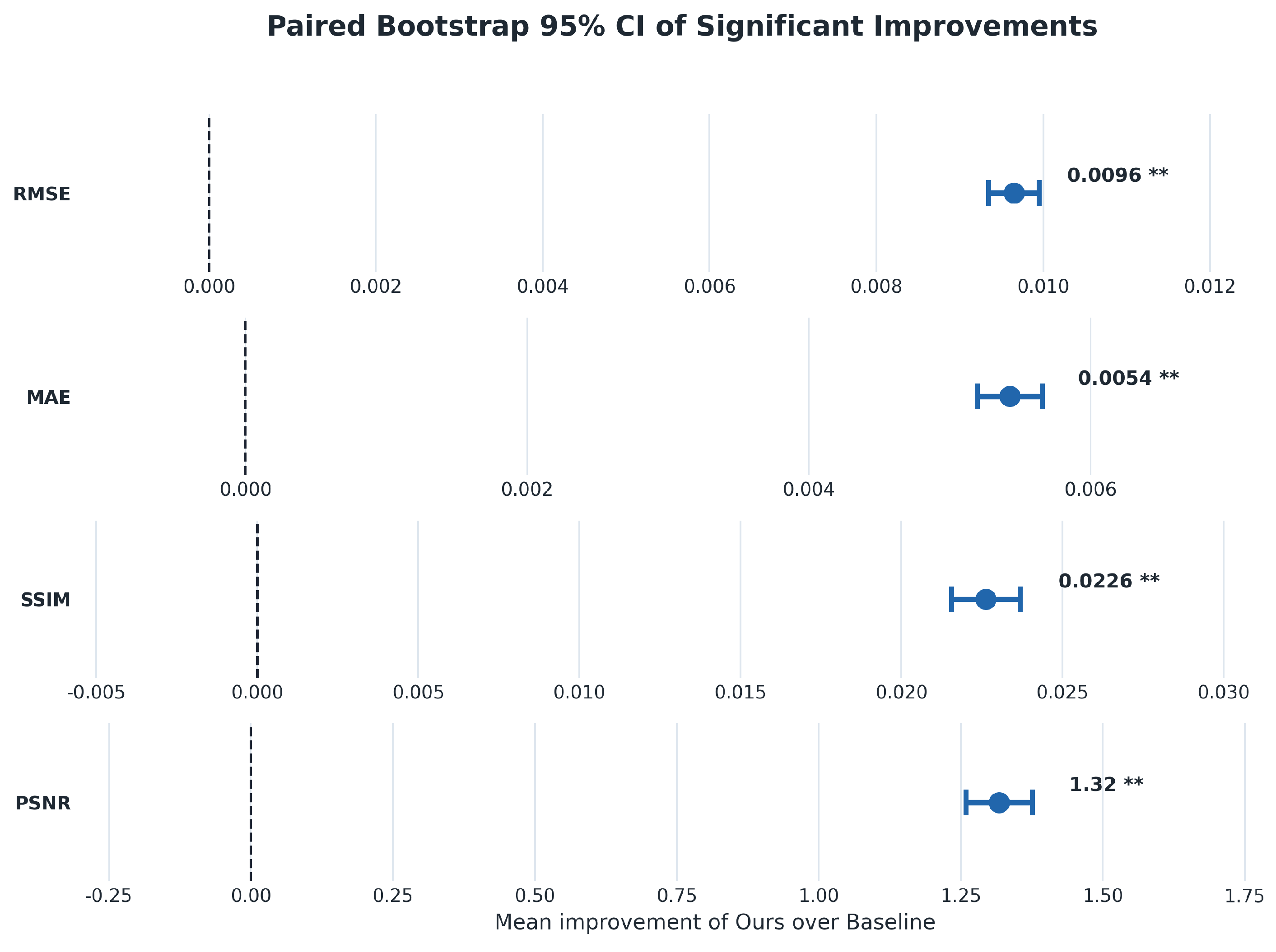
To further examine whether the performance improvement of the proposed method over competitive models is statistically reliable, this study adopts the paired bootstrap method to conduct confidence interval analysis on the main evaluation metrics. Since some comparison models in the aforementioned experiments already represent strong suboptimal models except for the proposed method, this section selects representative strong competitive models as references to more strictly evaluate the improvement stability of the proposed method across different test samples. Specifically, repeated resampling is performed on the test samples, and the average improvements of the proposed method over the reference model in terms of SSIM, PSNR, MAE, and RMSE, together with their $95\%$ confidence intervals, are calculated. The results are shown in Figure 8.

Unlike comparisons based only on mean results, paired bootstrap analysis can further reflect the stability of model performance improvements at the sample level. As shown in Figure 8, the $95\%$ confidence intervals corresponding to the four metrics, including SSIM, PSNR, MAE, and RMSE, are all located on the right side of the zero reference line. This indicates that the improvements of the proposed method over the reference model are not caused by accidental fluctuations in a small number of samples, but remain consistently advantageous in most resampled test subsets. Among them, the positive improvements in SSIM and PSNR indicate that the model achieves stable gains in spatial structure preservation and overall reconstruction quality. The improvements in MAE and RMSE further suggest that the proposed method can continuously reduce both average errors and large local errors. These results statistically support the effectiveness of the joint modeling strategy formed by TDIM, RGFM, and STB Loss in groundwater quality risk prediction, demonstrating that the model not only performs better in overall metrics but also has strong sample-level stability and statistical reliability.

5.8. Hyperparameter Sensitivity Experimental Results

To analyze the influence of different hyperparameter settings on model prediction performance, this study further conducts hyperparameter sensitivity experiments. The experiments mainly include three aspects: the STB Loss weight, input noise intensity, and learning rate, which are used to investigate the effects of boundary constraint strength, data perturbation, and optimization step size on the model, respectively. All experiments are conducted using the same data split, model architecture, and evaluation metrics to ensure the comparability of results under different settings.

5.8.1. Sensitivity Analysis of the STB Loss Weight

STB Loss is used to constrain the spatial boundaries and temporal variation boundaries of groundwater quality risk maps, and its weight affects the contribution of this constraint term to the overall optimization objective. To analyze the influence of boundary constraint strength on prediction performance, this study sets different STB Loss weights for comparative experiments. The results are shown in

Table 5. Sensitivity analysis of the STB loss weight.

STB Weight	SSIM ↑	PSNR ↑	MAE ↓	RMSE ↓
$0.1$	$0.9692\pm 0.0097$	$38.92\pm 1.90$	$4.32\times {10}^{-3}\pm 1.57\times {10}^{-3}$	$1.19\times {10}^{-2}\pm 2.92\times {10}^{-3}$
$0.3$	$0.9767\pm 0.0088$	$39.94\pm 1.44$	$3.36\times {10}^{-3}\pm 1.81\times {10}^{-3}$	$1.01\times {10}^{-2}\pm 1.37\times {10}^{-3}$
$0.5$	$\mathbf{0}.\mathbf{9814}\pm \mathbf{0}.\mathbf{0085}$	$\mathbf{40}.\mathbf{47}\pm \mathbf{2}.\mathbf{19}$	$\mathbf{2}.\mathbf{80}\times {\mathbf{10}}^{-\mathbf{3}}\pm \mathbf{1}.\mathbf{50}\times {\mathbf{10}}^{-\mathbf{3}}$	$\mathbf{9}.\mathbf{70}\times {\mathbf{10}}^{-\mathbf{3}}\pm \mathbf{2}.\mathbf{69}\times {\mathbf{10}}^{-\mathbf{3}}$
$0.7$	$0.9781\pm 0.0075$	$39.95\pm 2.18$	$2.89\times {10}^{-3}\pm 1.65\times {10}^{-3}$	$1.06\times {10}^{-2}\pm 2.17\times {10}^{-3}$
$1.0$	$0.9723\pm 0.0068$	$39.02\pm 1.83$	$3.96\times {10}^{-3}\pm 1.11\times {10}^{-3}$	$1.16\times {10}^{-2}\pm 2.29\times {10}^{-3}$

.

As shown in Table 5, changes in the STB Loss weight have a certain influence on model performance, indicating that spatiotemporal boundary constraints play a practical role in groundwater quality risk prediction. When the weight is within a moderate range, the model can achieve a better balance between structural preservation and numerical reconstruction. When the weight is too low, the boundary constraint is insufficient, making it difficult to fully preserve spatial transitions and local variations in the risk map. When the weight is too high, the model may overemphasize gradient boundaries and weaken its ability to fit the overall risk field. Overall, the model performance changes relatively smoothly under different weight settings without severe degradation, indicating that the proposed method has a certain robustness to the STB Loss weight.

5.8.2. Sensitivity Analysis Under Different Noise Intensities

Groundwater monitoring data may be affected by sampling errors, local outliers, and spatial interpolation errors. Therefore, it is necessary to evaluate the stability of the model under input perturbations. In this study, different intensities of noise are added to the input data to analyze the sensitivity of the model to data perturbations. The results are shown in

Table 6. Sensitivity analysis under different noise intensities.

Noise	SSIM ↑	PSNR ↑	MAE ↓	RMSE ↓
$0.00$	$\mathbf{0}.\mathbf{9814}\pm \mathbf{0}.\mathbf{0085}$	$\mathbf{40}.\mathbf{47}\pm \mathbf{2}.\mathbf{19}$	$\mathbf{2}.\mathbf{80}\times {\mathbf{10}}^{-\mathbf{3}}\pm \mathbf{1}.\mathbf{50}\times {\mathbf{10}}^{-\mathbf{3}}$	$\mathbf{9}.\mathbf{70}\times {\mathbf{10}}^{-\mathbf{3}}\pm \mathbf{2}.\mathbf{69}\times {\mathbf{10}}^{-\mathbf{3}}$
$0.01$	$0.9780\pm 0.0100$	$39.48\pm 1.65$	$3.34\times {10}^{-3}\pm 1.42\times {10}^{-3}$	$1.03\times {10}^{-2}\pm 1.35\times {10}^{-3}$
$0.03$	$0.9774\pm 0.0124$	$39.60\pm 0.90$	$3.73\times {10}^{-3}\pm 1.32\times {10}^{-3}$	$1.10\times {10}^{-2}\pm 2.74\times {10}^{-3}$
$0.05$	$0.9690\pm 0.0122$	$38.66\pm 2.10$	$4.25\times {10}^{-3}\pm 1.74\times {10}^{-3}$	$1.20\times {10}^{-2}\pm 1.65\times {10}^{-3}$
$0.07$	$0.9576\pm 0.0100$	$38.05\pm 1.52$	$5.20\times {10}^{-3}\pm 8.99\times {10}^{-4}$	$1.33\times {10}^{-2}\pm 1.37\times {10}^{-3}$
$0.10$	$0.9461\pm 0.0062$	$36.76\pm 2.18$	$6.39\times {10}^{-3}\pm 2.01\times {10}^{-3}$	$1.54\times {10}^{-2}\pm 2.56\times {10}^{-3}$

.

As shown in Table 6, model performance generally decreases as the noise intensity increases, indicating that the quality of input data still affects the accuracy of groundwater quality risk prediction. However, under low to moderate noise perturbations, the model can still maintain relatively high SSIM and PSNR values and relatively low error levels, suggesting that it can use temporal context and regional correlation information to alleviate the influence of local perturbations. When the noise intensity further increases, the spatial risk structure and local boundaries are more obviously damaged, leading to gradually increased prediction errors. Overall, although noise affects the model, the proposed method still maintains stable prediction performance within a certain perturbation range, demonstrating good anti-noise robustness.

5.8.3. Sensitivity Analysis of the Learning Rate

The learning rate determines the step size of model parameter updates and is an important factor affecting the training stability and convergence state of deep models. To analyze the sensitivity of the optimization process to learning rate variations, this study sets several typical learning rates for comparative experiments. The results are shown in

Table 7. Sensitivity analysis of the learning rate.

Learning Rate	SSIM ↑	PSNR ↑	MAE ↓	RMSE ↓
$1\times {10}^{-5}$	$0.9607\pm 0.0094$	$38.63\pm 1.99$	$4.78\times {10}^{-3}\pm 9.66\times {10}^{-4}$	$1.17\times {10}^{-2}\pm 2.52\times {10}^{-3}$
$3\times {10}^{-5}$	$0.9741\pm 0.0114$	$39.43\pm 1.72$	$3.35\times {10}^{-3}\pm 1.26\times {10}^{-3}$	$1.05\times {10}^{-2}\pm 2.63\times {10}^{-3}$
$1\times {10}^{-4}$	$\mathbf{0}.\mathbf{9814}\pm \mathbf{0}.\mathbf{0085}$	$\mathbf{40}.\mathbf{47}\pm \mathbf{2}.\mathbf{19}$	$\mathbf{2}.\mathbf{80}\times {\mathbf{10}}^{-\mathbf{3}}\pm \mathbf{1}.\mathbf{50}\times {\mathbf{10}}^{-\mathbf{3}}$	$\mathbf{9}.\mathbf{70}\times {\mathbf{10}}^{-\mathbf{3}}\pm \mathbf{2}.\mathbf{69}\times {\mathbf{10}}^{-\mathbf{3}}$
$3\times {10}^{-4}$	$0.9780\pm 0.0088$	$39.84\pm 1.77$	$3.32\times {10}^{-3}\pm 2.16\times {10}^{-3}$	$9.93\times {10}^{-3}\pm 2.02\times {10}^{-3}$
$1\times {10}^{-3}$	$0.9491\pm 0.0111$	$37.62\pm 1.50$	$6.00\times {10}^{-3}\pm 1.64\times {10}^{-3}$	$1.45\times {10}^{-2}\pm 3.17\times {10}^{-3}$

.

As shown in Table 7, changes in the learning rate affect the optimization performance of the model, but the model still maintains good performance stability within adjacent learning rate ranges. When the learning rate is too small, the parameter update magnitude is limited, and the model cannot sufficiently learn complex spatiotemporal features and regional risk variations. When the learning rate is too large, the parameter update process tends to become unstable, making it difficult for the model to finely characterize local structures and boundary changes in groundwater quality risk maps. Within the medium learning rate range, SSIM, PSNR, MAE, and RMSE all remain at relatively good levels, indicating that the proposed model is not extremely sensitive to the learning rate. Overall, the learning rate affects the training convergence quality, but the proposed model has good optimization robustness within a reasonable learning rate range.

5.9. Error Distribution and Cumulative Error Analysis

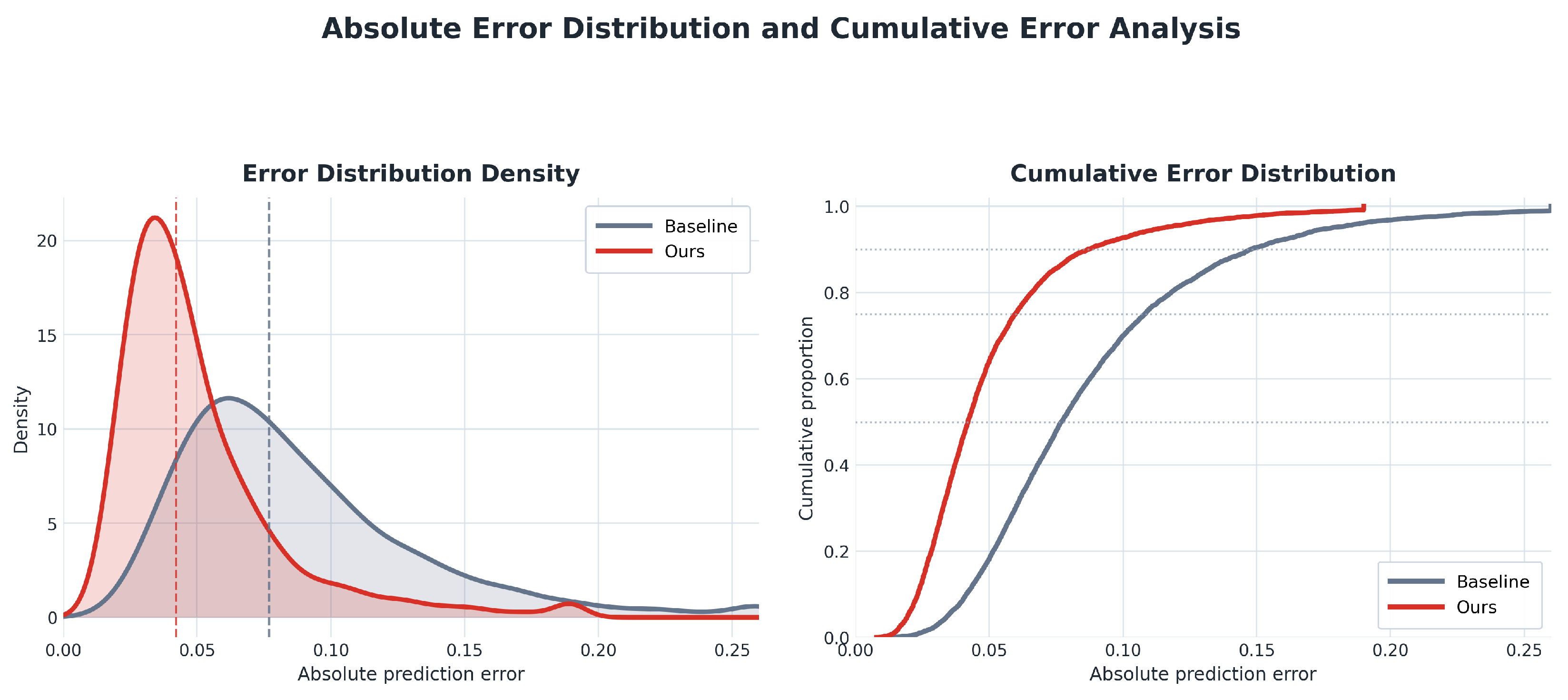
To further analyze the distribution characteristics of model errors in the test samples, this study performs kernel density estimation and cumulative distribution statistics on the absolute errors of the prediction results. In this section, the baseline model is selected as the reference to more clearly observe the differences between the proposed method and the baseline model in terms of error concentration and large-error control. The absolute error distribution and cumulative error statistics are shown in Figure 9.

The error distribution can reveal the structure of prediction deviations beyond average metrics. As shown in Figure 9, the error density peak of the proposed method is closer to the zero-error region, and the distribution is more concentrated, indicating that the prediction deviations of most grid cells are compressed within a smaller range. In contrast, the error distribution of the baseline shifts to the right overall and shows a more obvious long-tail characteristic, suggesting that it is more likely to produce large local prediction deviations. From the cumulative distribution curves, the proposed method covers a higher proportion of samples under smaller error thresholds, indicating that its prediction errors are not only lower in mean value but also contain a higher proportion of small-error samples. This phenomenon shows that the proposed model does not simply reduce the errors of a small number of samples, but improves prediction stability across the entire grid range, making the error distribution more compact and thereby benefiting subsequent regional risk identification and water environmental safety zoning.

5.10. Held-Out Monitoring-Site Quantitative Validation

To further evaluate the prediction accuracy of the proposed model against actual groundwater monitoring observations, an additional five-fold monitoring-site-level validation experiment was conducted. A total of 1084 valid groundwater monitoring records were included in this experiment. These records were first grouped according to their corresponding monitoring-site identities, and all valid monitoring sites were then divided into five non-overlapping subsets using a fixed site-level split. In each fold, one subset of monitoring sites was completely held out, and all monitoring records and temporal observations associated with these held-out sites were excluded before indicator normalization, IDW interpolation, nearest-neighbor completion, and model training, thereby ensuring that no information from the held-out monitoring locations participated in the construction of the model inputs or training targets. The monitoring records from the remaining sites were used to construct the monthly groundwater quality risk maps following the same data-processing procedure as the main experiment.

The resulting monthly sequences were further divided chronologically into training, validation, and test periods using the same 7:1:2 ratio as the main experiment, without random temporal shuffling or cross-subset temporal-window construction. After prediction, the groundwater quality risk values at the geographical coordinates of the held-out monitoring sites were extracted from the predicted maps and directly compared with the integrated risk values calculated from the corresponding actual groundwater monitoring observations. This procedure was repeated for all five subsets so that each monitoring site was used as an independent held-out spatial location in one of the five folds. Since this experiment evaluates point-level prediction against actual monitoring observations rather than image-level spatial reconstruction, MAE, RMSE, and $R^2$ were used as the quantitative evaluation metrics. The same held-out-site partitions, temporal splits, preprocessing procedures, and evaluation protocol were used for both the Baseline and the proposed model to ensure a fair comparison.

Table 8. Quantitative comparison on held-out groundwater monitoring-site observations. The results are reported as mean ± standard deviation over five monitoring-site-level folds.

Method	MAE ↓	RMSE ↓	${\mathit{R}}^2$↑
Baseline	$0.0223\pm 0.0017$	$0.0312\pm 0.0018$	$0.8433\pm 0.0265$
Ours	$\mathbf{0}.\mathbf{0141}\pm \mathbf{0}.\mathbf{0010}$	$\mathbf{0}.\mathbf{0209}\pm \mathbf{0}.\mathbf{0013}$	$\mathbf{0}.\mathbf{9295}\pm \mathbf{0}.\mathbf{0129}$

presents the quantitative validation results against the observations from the held-out groundwater monitoring sites. The proposed method consistently outperforms the Baseline across all evaluation metrics, showing lower point-level prediction errors and a stronger agreement between the predicted groundwater quality risk values and those calculated from the actual monitoring observations. Moreover, the smaller variations across the monitoring-site-level folds indicate that the proposed model maintains more stable predictive performance when different spatial subsets of monitoring sites are excluded from interpolation and training. These results further demonstrate that the performance improvement is not limited to reproducing interpolation-derived regional risk maps, but is also retained when the model is directly evaluated against actual observations from previously unseen monitoring locations.

5.11. Local-Scale Application Analysis

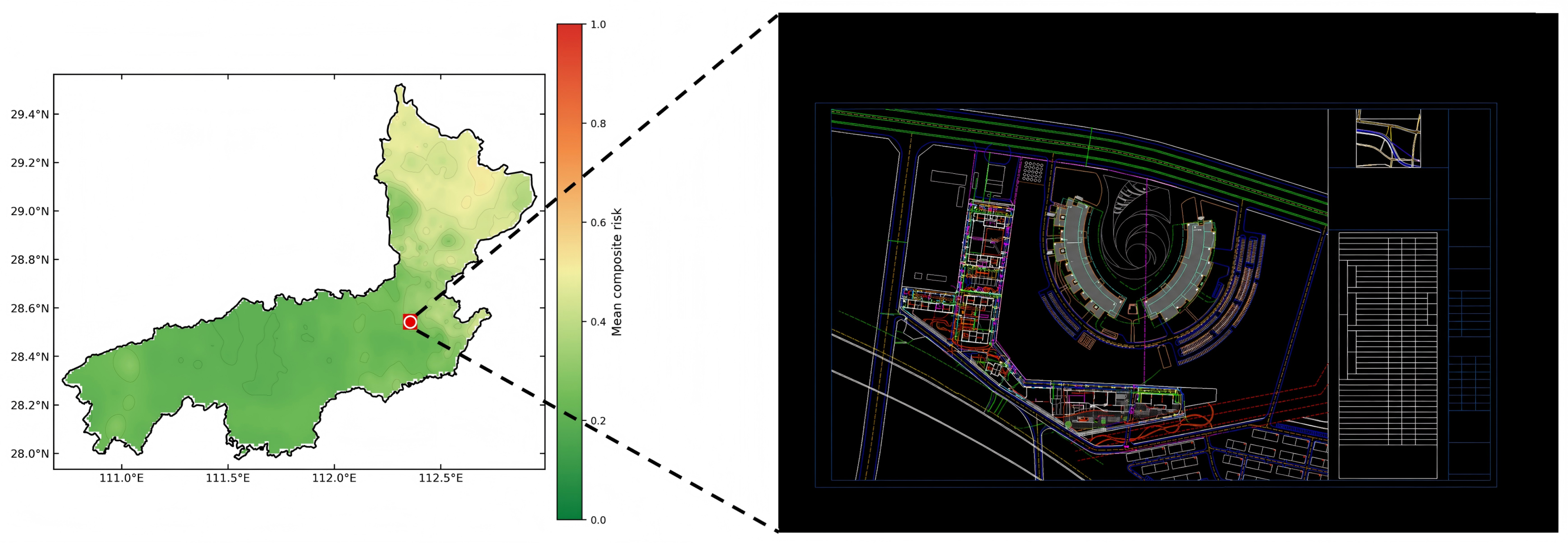
To further examine the local-scale applicability of the proposed model, this study selects a residential community in Yiyang City as a typical local application area and conducts local-scale visual and quantitative analysis of the model prediction results. This area has a clear engineering application background and underground space modeling requirements, and can be used to examine the interpretability of regional-scale groundwater quality prediction results in specific urban construction units. An example image of the selected residential community is shown in Figure 10.

By marking the location of the residential community on the groundwater quality risk prediction map, the spatial correspondence between the model prediction results and the real application area can be further analyzed, thereby providing support for subsequent urban geological modeling, water environmental safety assessment, and local risk identification. The experimental results are presented here, as shown in

Table 9. Quantitative results within the selected residential community area. The results are reported as mean ± standard deviation.

Method	SSIM ↑	PSNR ↑	MAE ↓	RMSE ↓
Baseline	$0.9447\pm 0.0128$	$36.18\pm 1.57$	$7.26\times {10}^{-3}\pm 1.94\times {10}^{-3}$	$1.58\times {10}^{-2}\pm 3.27\times {10}^{-3}$
Ours	$\mathbf{0}.\mathbf{9789}\pm \mathbf{0}.\mathbf{0076}$	$\mathbf{39}.\mathbf{86}\pm \mathbf{1}.\mathbf{72}$	$\mathbf{3}.\mathbf{18}\times {\mathbf{10}}^{-\mathbf{3}}\pm \mathbf{1}.\mathbf{37}\times {\mathbf{10}}^{-\mathbf{3}}$	$\mathbf{9}.\mathbf{84}\times {\mathbf{10}}^{-\mathbf{3}}\pm \mathbf{2}.\mathbf{41}\times {\mathbf{10}}^{-\mathbf{3}}$

.

As shown in Table 9, within the selected residential community area, the proposed method outperforms the Baseline on all four metrics, including SSIM, PSNR, MAE, and RMSE. This indicates that the model still maintains good prediction stability and spatial adaptability at the local spatial scale. Specifically, the proposed method achieves higher SSIM and PSNR, demonstrating that it can more accurately preserve the spatial structure and overall reconstruction quality of groundwater quality risk maps around the residential community. Meanwhile, its MAE and RMSE are clearly lower than those of the Baseline, indicating that the proposed method can reduce both the average prediction deviation and large errors within the local area. These results further show that the performance advantages observed at the regional scale are also maintained within the selected local area, indicating the potential of the predicted groundwater quality risk maps to provide spatial reference information for local risk identification, underground space development, urban geological modeling, and water environmental safety assessment.

6. Discussion

This study focuses on the problem of spatiotemporal groundwater quality prediction under multi-indicator coupling constraints and constructs a complete modeling workflow from multi-source water quality indicator normalization, integrated risk index generation, and regional gridded representation to deep spatiotemporal prediction. The experimental results show that the proposed model can effectively capture the continuous evolution characteristics of groundwater quality risk in the temporal dimension and the heterogeneous distribution patterns in the spatial dimension. Specifically, TDIM enhances the model’s ability to represent adjacent-month variations and multi-timescale cumulative effects, RGFM improves the model’s response capability to high-risk regions, boundary regions, and spatially heterogeneous areas, and STB Loss further constrains the spatial boundaries and temporal variation consistency of the prediction results. From the perspective of practical application, the proposed method can transform discrete groundwater monitoring site data into continuous regional risk maps, providing auxiliary support for dynamic groundwater quality monitoring, risk zoning, pollution warning, and urban geological modeling. In particular, in the residential community application scenario, the model prediction results can establish spatial correspondence with specific urban construction units, which helps provide a more intuitive decision-making basis for underground space development, water environmental safety assessment, and local risk identification.

Although the proposed method achieves good experimental results, it still has certain limitations. First, the data used in this study mainly come from monthly observation records of groundwater monitoring sites. The uneven spatial distribution of monitoring sites and insufficient samples in local areas may affect the fine-grained representation ability of gridded risk maps. Especially in sparsely monitored regions, the interpolation results may still contain uncertainty. In addition, although invalid cells outside the administrative boundary are excluded using a spatial mask during data construction, loss calculation, and quantitative evaluation, conventional convolution and downsampling operations may still introduce limited feature mixing near the irregular study-area boundary. Future work will investigate mask-aware convolution or boundary-adaptive feature propagation to further reduce this influence. In addition, although the dataset spans a relatively long period from 2000 to 2023, it contains only 288 monthly observations, and the limited number of temporal samples may increase the risk of overfitting for a relatively complex spatiotemporal model and constrain its generalization ability to unseen temporal periods or other study regions. Second, the integrated risk index in this study is mainly constructed based on existing water quality indicators. Although it can unify the risk directions and numerical scales of different indicators, external driving factors such as groundwater depth, aquifer structure, land use, human activity intensity, precipitation, and topography have not yet been further introduced. Therefore, there is still room for improving the interpretation of complex hydrogeological processes. In addition, the current model mainly focuses on one-step-ahead prediction. Future research can further extend the model to multi-step prediction, cross-region transfer, and uncertainty quantification, so as to improve its generalization ability in long-term risk warning and applications across different urban regions. In the future, more field verification data and three-dimensional urban geological models can also be integrated to achieve deeper fusion between groundwater quality prediction results and underground space development, geological safety assessment, and urban planning management.

7. Conclusions

To address the challenges of groundwater quality being affected by multi-indicator coupling, uneven spatial distribution, and complex temporal variation processes, this study proposes a spatiotemporal deep learning model for regional integrated groundwater quality risk prediction. First, an integrated groundwater quality risk index is constructed based on dissolved oxygen, total nitrogen, electrical conductivity, dissolved organic carbon, pH, permanganate index, and total phosphorus. Then, monthly regional spatiotemporal sequences are generated through spatial interpolation and gridded processing. On this basis, the model captures multi-scale temporal variations in groundwater quality risk through TDIM, strengthens the representation of risk correlations among different spatial regions through RGFM, and constrains the spatial boundaries and temporal variation consistency of the prediction results using STB Loss. The experimental results show that the proposed method outperforms multiple comparison models in terms of SSIM, PSNR, MAE, and RMSE, and demonstrates good prediction accuracy, stability, and application interpretability in ablation experiments, hyperparameter sensitivity analysis, error distribution analysis, and residential community application analysis. Overall, the proposed method can provide effective technical support for regional groundwater quality dynamic prediction, water environmental safety assessment, and urban-scale local risk identification.

References

1. Ram, A.; Tiwari, S.K.; Pandey, H.K.; Chaurasia, A.K.; Singh, S.; Singh, Y.V. Groundwater quality assessment using water quality index (WQI) under GIS framework. Appl. Water Sci. 2021, 11, 46. [Google Scholar] [CrossRef] [Scilit]
2. Piyathilake, I.D.U.H.; Ranaweera, L.V.; Udayakumara, E.P.N.; Gunatilake, S.K.; Dissanayake, C.B. Assessing groundwater quality using the water quality index (WQI) and GIS in the Uva Province, Sri Lanka. Appl. Water Sci. 2022, 12, 72. [Google Scholar] [CrossRef] [Scilit]
3. Adimalla, N.; Li, P.; Venkatayogi, S. Hydrogeochemical evaluation of groundwater quality for drinking and irrigation purposes and integrated interpretation with water quality index studies. Environ. Process. 2018, 5, 363–383. [Google Scholar] [CrossRef] [Scilit]
4. Bhunia, G.S.; Keshavarzi, A.; Shit, P.K.; Omran, E.S.E.; Bagherzadeh, A. Evaluation of groundwater quality and its suitability for drinking and irrigation using GIS and geostatistics techniques in semiarid region of Neyshabur, Iran. Appl. Water Sci. 2018, 8, 168. [Google Scholar] [CrossRef] [Scilit]
5. Tesema, A.; Jothimani, M.; Abebe, A.; Gunalan, J.; Getahun, E.; Karuppannan, S. Hydrochemical characterization and water quality assessment for drinking and irrigation purposes using WQI and GIS techniques in the Upper Omo River Basin, Southern Ethiopia. J. Chem. 2023, 2023, 3246851. [Google Scholar] [CrossRef] [Scilit]
6. Pyo, J.; Pachepsky, Y.; Kim, S.; Abbas, A.; Kim, M.; Kwon, Y.S.; Ligaray, M.; Cho, K.H. Long short-term memory models of water quality in inland water environments. Water Res. X 2023, 21, 100207. [Google Scholar] [CrossRef] [Scilit]
7. Sajib, A.M.; Bamal, A.; Diganta, M.T.M.; Ashekuzzaman, S.; Rahman, A.; Olbert, A.I.; Uddin, M.G. Novel groundwater quality index (GWQI) model: A reliable approach for the assessment of groundwater. Results Eng. 2025, 25, 104265. [Google Scholar] [CrossRef] [Scilit]
8. Cauich-Kau, D.; Castro-Larragoitia, J.; Benavides, A.C.; García-Arreola, M.E.; García-Vargas, G.G. An adapted groundwater quality index including toxicological critical pollutants. Groundw. Sustain. Dev. 2025, 28, 101401. [Google Scholar] [CrossRef] [Scilit]
9. Zhang, B.; Hu, X.; Li, B.; Wu, P.; Cai, X.; Luo, Y.; Deng, X.; Jiang, M. A Groundwater Quality Assessment Model for Water Quality Index: Combining Principal Component Analysis, Entropy Weight Method, and Coefficient of Variation Method for Dimensionality Reduction and Weight Optimization, and Its Application. Water Environ. Res. 2024, 96, e11155. [Google Scholar] [CrossRef] [Scilit]
10. Das, C.R.; Som, R.; Das, S. Transforming water safety: A comprehensive groundwater quality index for reliable drinking water in South 24 Parganas, India. Reg. Stud. Mar. Sci. 2025, 92, 104628. [Google Scholar] [CrossRef] [Scilit]
11. Boukich, O.; Ben-tahar, R.; El guerrouj, B.; Smiri, Y. New approach to evaluate groundwater quality for human consumption: Application of a personalized index and health risk assessment of potentially toxic elements. Groundw. Sustain. Dev. 2025, 31, 101542. [Google Scholar] [CrossRef] [Scilit]
12. Basharat, U.; Zhang, W.; Abbasi, A.; Mahroof, S.; Han, C.; Khan, S.H.; Li, S. Integrated assessment of groundwater hydrogeochemistry and quality using multivariate statistical analysis, self-organizing maps, and water quality indices in District Bagh, AJK, Pakistan. Ecotoxicol. Environ. Saf. 2025, 301, 118515. [Google Scholar] [CrossRef] [Scilit]
13. Kalaivanan, K.; Karunanidhi, D.; Sankar, K.; Marghade, D.; Subramani, T.; Shanthi, D. Groundwater quality and nitrate health risk evaluation in eastern part of Salem district, south India: Insights from water quality index (WQI) and GIS techniques. J. Environ. Chem. Eng. 2025, 13, 118609. [Google Scholar] [CrossRef] [Scilit]
14. Nafouanti, M.B.; Li, J.; Usman, U.S.; Mwakipunda, G.C.; Fatima, E.B.; Baba, A.S. Groundwater quality prediction using novel hybrid classification and regression models. J. Contam. Hydrol. 2025, 277, 104834. [Google Scholar] [CrossRef] [Scilit]
15. Sundhar, S.; Shashannk, S.; Nandhini, D.; Amutha, S. Ground water quality assessment and forecasting using attention-based mechanisms. Environ. Sci. Eur. 2025, 37, 232. [Google Scholar] [CrossRef] [Scilit]
16. Rostami, A.A.; Sedghi, Z.; Nadiri, A.A.; Barzegar, R.; Dimova, N.T.; Senapathi, V.; Islam, A.R.M.T. Harnessing deep learning for fusion-based heavy metal contamination index prediction in groundwater. J. Contam. Hydrol. 2025, 274, 104672. [Google Scholar] [CrossRef] [Scilit]
17. Hasan, M.A.; Basak, S.B.; Haque, M.K.; Roy, S.K. Comprehensive assessment of groundwater quality in Moilakanda, Mymensingh City: Insights from water quality indices and multivariate analysis. Clean. Water 2026, 5, 100148. [Google Scholar] [CrossRef] [Scilit]
18. Valadkhan, D.; Moghaddasi, R.; Mohammadinejad, A. Groundwater quality prediction based on LSTM RNN: An Iranian experience. Int. J. Environ. Sci. Technol. 2022, 19, 11397–11408. [Google Scholar] [CrossRef] [Scilit]
19. Liu, C.; Xu, M.; Liu, Y.; Li, X.; Pang, Z.; Miao, S. Predicting groundwater indicator concentration based on long short-term memory neural network: A case study. Int. J. Environ. Res. Public Health 2022, 19, 15612. [Google Scholar] [CrossRef] [Scilit]
20. Kouadri, S.; Pande, C.B.; Panneerselvam, B.; Moharir, K.N.; Elbeltagi, A. Prediction of irrigation groundwater quality parameters using ANN, LSTM, and MLR models. Environ. Sci. Pollut. Res. 2022, 29, 21067–21091. [Google Scholar] [CrossRef] [Scilit]
21. Rammohan, B.; Partheeban, P.; Ranganathan, R.; Balaraman, S. Groundwater quality prediction and analysis using machine learning models and geospatial technology. Sustainability 2024, 16, 9848. [Google Scholar] [CrossRef] [Scilit]
22. Li, X.; Liang, G.; He, B.; Ning, Y.; Yang, Y.; Wang, L.; Wang, G. Recent advances in groundwater pollution research using machine learning from 2000 to 2023: A bibliometric analysis. Environ. Res. 2025, 267, 120683. [Google Scholar] [CrossRef] [Scilit]
23. He, Y.; Duan, Z.L.; Ding, X.H.; Zhang, Z.; Mayoulou, R.E.; Zhu, K.F. Spatiotemporal prediction for groundwater heavy metal contamination using Soft-DTW-based clustering and graph neural network framework. Water Res. 2025, 291, 125245. [Google Scholar] [CrossRef] [Scilit]
24. Qiao, F.; Wang, J.; Song, J.; Chen, Z.; Kwaw, A.K.; Zhao, Y.; Zheng, S. The spatiotemporal evolution of dissolved-phase NAPL plumes revealed by the integrated groundwater quality and machine learning models. Water Res. 2025, 280, 123535. [Google Scholar] [CrossRef] [Scilit]
25. Selvarangam, D.K.; Jayalakshmi, S.; Ramakrishnan, S.S. Prediction of nitrate and sulphate dynamics in groundwater under spatiotemporal effects of urban growth using attention optimized models. Sci. Rep. 2025, 15, 39760. [Google Scholar] [CrossRef] [Scilit]
26. Zhu, Y.; Liu, Q. Toward transparent groundwater contamination risk forecasting: Integrating causal discovery and Bayesian graph neural networks. Sci. Total Environ. 2025, 998, 180233. [Google Scholar] [CrossRef] [Scilit]
27. Taccari, M.L.; Wang, H.; Nuttall, J.; Chen, X.; Jimack, P.K. Spatial-temporal graph neural networks for groundwater data. Sci. Rep. 2024, 14, 24564. [Google Scholar] [CrossRef] [Scilit]
28. Han, Z.; Li, F.; Zhao, Y.; Liu, C. Investigation into groundwater level prediction within a deep learning framework: Incorporating the spatial dynamics of adjacent wells. J. Hydrol. 2025, 657, 133097. [Google Scholar] [CrossRef] [Scilit]
29. Tran, D.; Bourdev, L.; Fergus, R.; Torresani, L.; Paluri, M. Learning spatiotemporal features with 3D convolutional networks. In Proceedings of the IEEE International Conference on Computer Vision, Santiago, Chile, 7–13 December 2015. [Google Scholar]
30. Wang, Y.; Long, M.; Wang, J.; Gao, Z.; Yu, P.S. Predrnn: Recurrent neural networks for predictive learning using spatiotemporal lstms. Adv. Neural Inf. Process. Syst. 2017, 30, 879–888. [Google Scholar]
31. Tang, S.; Li, C.; Zhang, P.; Tang, R. Swinlstm: Improving spatiotemporal prediction accuracy using swin transformer and lstm. In Proceedings of the IEEE/CVF International Conference on Computer Vision, Paris, France, 1–6 October 2023; pp. 13470–13479. [Google Scholar]
32. Yuan, Y.; Ding, J.; Feng, J.; Jin, D.; Li, Y. Unist: A prompt-empowered universal model for urban spatio-temporal prediction. In Proceedings of the 30th ACM SIGKDD Conference on Knowledge Discovery and Data Mining, Barcelona, Spain, 25–29 August 2024; pp. 4095–4106. [Google Scholar]
33. Zhang, Z.; Huang, Z.; Hu, Z.; Zhao, X.; Wang, W.; Liu, Z.; Zhang, J.; Qin, S.J.; Zhao, H. Mlpst: Mlp is all you need for spatio-temporal prediction. In Proceedings of the 32nd ACM International Conference on Information and Knowledge Management, Birmingham, UK, 21–25 October 2023; pp. 3381–3390. [Google Scholar]
34. Yu, C.; Wang, F.; Wang, Y.; Shao, Z.; Sun, T.; Yao, D.; Xu, Y. Mgsfformer: A multi-granularity spatiotemporal fusion transformer for air quality prediction. Inf. Fusion 2025, 113, 102607. [Google Scholar] [CrossRef] [Scilit]
35. Tan, C.; Gao, Z.; Li, S.; Li, S.Z. SimVPv2: Towards simple yet powerful spatiotemporal predictive learning. IEEE Trans. Multimed. 2025, 27, 5170–5184. [Google Scholar] [CrossRef] [Scilit]
36. Tang, Y.; Dong, P.; Tang, Z.; Chu, X.; Liang, J. Vmrnn: Integrating vision mamba and lstm for efficient and accurate spatiotemporal forecasting. In Proceedings of the IEEE/CVF Conference on Computer Vision and Pattern Recognition, Seattle, WA, USA, 16–22 June 2024; pp. 5663–5673. [Google Scholar]
37. Tan, C.; Li, S.; Gao, Z.; Guan, W.; Wang, Z.; Liu, Z.; Wu, L.; Li, S.Z. Openstl: A comprehensive benchmark of spatio-temporal predictive learning. Adv. Neural Inf. Process. Syst. 2023, 36, 69819–69831. [Google Scholar] [CrossRef] [Scilit]
38. Chang, Z.; Zhang, X.; Wang, S.; Ma, S.; Gao, W. Strpm: A spatiotemporal residual predictive model for high-resolution video prediction. In Proceedings of the IEEE/CVF Conference on Computer Vision and Pattern Recognition, New Orleans, LA, USA, 18–22 June 2022; pp. 13946–13955. [Google Scholar]
39. Yuan, Y.; Ding, J.; Han, C.; Sheng, Z.; Jin, D.; Li, Y. UniFlow: A foundation model for unified urban spatio-temporal flow prediction. IEEE Trans. Mob. Comput. 2026, 25, 13034–13046. [Google Scholar] [CrossRef] [Scilit]
40. Cheng, J.; Nie, L.; Chen, S.Y.; Wang, Y.; Yang, Z.; Luo, Y. TSF-Mlstm: A Spatiotemporal Feature-Enhanced Monitoring Method for Coalmine Pressure Prediction. IEEE Trans. Instrum. Meas. 2026, 75, 9517113. [Google Scholar] [CrossRef] [Scilit]
41. Cao, H.; Leng, H.; Yan, Y.; Zhao, J.; Liu, Y.; Huang, L.; Chai, X.; Li, B. AMV-STECNet: A Deep Learning Framework for Spatiotemporal Error Correction of Atmospheric Motion Vectors to Enhance Numerical Weather Prediction. IEEE Trans. Geosci. Remote Sens. 2026, 64, 4101913. [Google Scholar] [CrossRef] [Scilit]
Figure 1. Overall architecture of the proposed spatiotemporal deep learning framework for regional groundwater quality composite safety index prediction.
Water 18 02219 g001
Figure 2. The TDIM module jointly models the temporal evolution process of groundwater quality features through the main feature stream, differential encoding stream, and motion-aware temporal aggregation stream. By incorporating adjacent differences, multi-lag differences, a temporal-difference pyramid, and a temporal gating mechanism, this module enhances the model ability to represent local abrupt changes, multi-interval temporal variations, and cross-temporal dynamic propagation relationships.
Water 18 02219 g002
Figure 3. The RGFM module constructs regional affinity relationships through multi-scale feature fusion, regional prior encoding, and feature token modeling, thereby enhancing the representation of associations among specific spatial units in groundwater quality prediction. Furthermore, this module uses normalized region-guided information to generate scaling and shifting parameters, which adaptively modulate the original features to highlight high-risk regions, significantly changing regions, and boundary transition areas.
Water 18 02219 g003
Figure 4. Dataset characterization of the groundwater quality monitoring data in the study area, including temporal coverage, spatial sampling density, indicator-level risk contribution, composite risk distribution, risk grade composition, and mean spatial risk pattern. The results show that the constructed dataset contains continuous temporal observations and clear spatial heterogeneity, providing a reliable data basis for regional groundwater quality spatiotemporal prediction and water environmental safety assessment.
Water 18 02219 g004
Figure 5. Training and validation loss curves over 200 epochs.
Water 18 02219 g005
Figure 6. Visual comparison of groundwater quality risk prediction maps generated by the proposed method and competitive baseline models.
Water 18 02219 g006
Figure 7. Residual visualization comparison between the proposed model and the baseline model for groundwater quality risk prediction.
Water 18 02219 g007
Figure 8. Paired bootstrap 95 % confidence intervals of the performance improvements achieved by the proposed method over the baseline model.
Water 18 02219 g008
Figure 9. Absolute error distribution and cumulative error comparison between the proposed method and the baseline model. The absolute errors were normalized for distribution visualization.
Water 18 02219 g009
Figure 10. Spatial localization of the selected residential community application area, showing the correspondence between the regional groundwater quality risk map and the target urban construction unit.
Water 18 02219 g010