Inversion of Groundwater DNAPL Pollution Source Based on DCNN Surrogate Model and Hybrid Homotopy-PSO with Feedback Iteration

Abstract

Existing DNAPL groundwater source inversion approaches are confronted with prominent bottlenecks: shallow surrogate models often fail to capture strong nonlinear multiphase flow relationships, traditional heuristic optimizers suffer from premature convergence, and ill-posed equifinality further degrades inversion reliability, together with prohibitive computational costs from repeated multiphase numerical simulation. Taking a typical chemical-contaminated site in Northeast China as the research object, this study establishes a multiphase flow numerical model that fully reproduces the migration and transformation mechanisms of chlorobenzene-based DNAPLs after systematic generalization of the site’s geological and hydrogeological conditions. To drastically cut the computational burden incurred during iterative inversion, high-quality datasets are generated via parameter sensitivity analysis and Latin hypercube sampling, based on which a deep convolutional neural network (DCNN)-driven high-fidelity surrogate model is constructed and embedded into the optimization framework as an equality constraint. A separated nonlinear programming model is formulated to independently quantify pollution source characteristics and hydrogeological parameters, with the objective of minimizing the residual error between field-measured and numerically simulated contaminant concentrations. A hybrid homotopy-particle swarm optimization (HH-PSO) algorithm is further proposed to address the limitations of conventional optimizers, including strong dependence on initial guesses and susceptibility to local optima. On this basis, a closed-loop feedback iteration scheme is developed, where source identification and parameter calibration are implemented alternately with bidirectional constraints and progressive correction to continuously refine and stabilize inversion outputs. This work presents distinct innovations in the methodology, algorithm, and practical application of DNAPL groundwater source inversion. Results from synthetic benchmark cases and on-site field applications demonstrate that the DCNN surrogate model achieves far higher fitting accuracy than shallow learning approaches (e.g., Kriging and support vector regression), with the coefficient of determination R² exceeding 0.99. After the feedback correction iteration procedure, the average relative error for retrieved source locations, release histories, and hydrogeological parameters drops to 3.72%, and the overall computational efficiency is elevated by approximately 99.84%. The integrated simulation–optimization inversion framework proposed in this work integrates monitoring signal denoising, multiphase numerical simulation, deep learning surrogate modeling, hybrid intelligent optimization, and feedback iterative correction. This integrated system effectively resolves core technical bottlenecks in DNAPL groundwater source inversion, such as nonlinear ill-posedness, equifinality induced by mutual interference between source terms and aquifer parameters, prohibitive computational costs of multiphase simulations, and premature convergence of traditional optimization algorithms. The established framework can serve as a robust theoretical foundation and technical tool for rapid, precise source tracing, pollution liability confirmation, and remediation design at complex contaminated sites.

1. Introduction

Leakage of petroleum-derived and chlorinated solvents during production, storage, transportation, and frequent usage of petrochemical products introduces dense non-aqueous phase liquids (DNAPLs) into the subsurface. Due to their high density, low solubility, high interfacial tension, and strong toxicity and persistence, DNAPLs remain trapped in aquifers over long periods and continuously release dissolved contaminants, posing severe threats to drinking water safety and ecosystem health. Unlike surface water pollution, groundwater contamination is highly concealed and often discovered only after extensive migration has occurred. Consequently, critical information including source location, release intensity, and historical release process cannot be directly observed, bringing enormous difficulties to pollution liability identification, risk management, and remediation design [1,2]. Therefore, developing efficient, stable, and high-precision methods for groundwater DNAPL pollution source inversion has become an urgent demand in groundwater resource protection and contaminated site management.

Mathematically, groundwater pollution source inversion represents a typical nonlinear ill-posed inverse problem [3,4]. Limited and noisy monitoring data, unknown model parameters, and unknown source conditions together lead to equifinality, where different parameter combinations can produce similar concentration fields, resulting in non-unique and unstable inversion results. Meanwhile, multiphase flow numerical models are structurally complex and computationally expensive; frequent calls during iterative inversion create prohibitive computational burdens [5]. Existing surrogate-based acceleration schemes and heuristic optimization algorithms still suffer from notable bottlenecks when coping with the strong nonlinearity of multiphase flow inversion tasks.

To overcome these difficulties, this study develops a simulation–optimization coupling model based on artificial intelligence to invert and trace DNAPL pollutants. The research focuses on four key components: establishing an adaptive wavelet threshold denoising method for noisy monitoring data [6,7]; constructing a high-precision DCNN surrogate for multiphase flow models to balance speed and accuracy [8]; proposing a hybrid homotopy-PSO algorithm that is independent of initial values for robust global optimization; and designing a separated identification and bidirectional correction feedback iteration scheme to suppress equifinality at the mechanism level [9]. Verified by both hypothetical and real-world cases, the proposed method significantly improves accuracy, stability, and efficiency, providing a reproducible and scalable paradigm for rapid source inversion at similar contaminated sites [10].

This study clarifies its main innovations from methodological, algorithmic, and application-oriented perspectives.

(1) Methodological innovation: An integrated end-to-end inversion framework, combining adaptive monitoring data denoising, DCNN surrogate modelling, and closed-loop feedback correction iteration, is established. A separated identification strategy is adopted to decouple pollution source characteristics and aquifer hydrogeological parameters. Bidirectional constraint and progressive correction are realized via closed-loop iteration, which effectively mitigates the equifinality effect and the ill-posed nature of DNAPL source inversion. DCNN is adapted as a high-precision surrogate for multiphase flow simulation, which greatly relieves the heavy computational burden caused by repeated multiphase model calls.

(2) Algorithmic innovation: A hybrid homotopy-particle swarm optimization (HH-PSO) algorithm is proposed. By combining the global path-tracking advantage of the homotopy method and the local searching capability of PSO, the algorithm reduces strong initial value dependence and alleviates the premature convergence problem of conventional PSO.

(3) Application-oriented innovation: The proposed integrated simulation–optimization framework is applied to a real-world chlorobenzene-contaminated DNAPL site in Northeast China. Real-site inversion simultaneously retrieves pollution source spatial location, the historical release process, and key hydrogeological parameters. It provides practical technical support for source tracing, pollution liability identification, and a groundwater remediation design for actual complex contaminated site scenarios.

2. Study Area and Multiphase Flow Numerical Model

2.1. Site Overview

A historically contaminated chemical site in Northeast China is selected as the real study area. The site has a long history of organic chemical production and storage, and historical leakage incidents have resulted in chlorobenzene contamination in the unconfined aquifer. The site is located on the second terrace of a river, with a relatively flat terrain, covered by silty clay and fine sand, underlain by impermeable granite forming a stable aquifer base. The aquifer thickness is approximately 10 m. Groundwater flows slowly from the northeast to the southwest, with a hydraulic gradient ranging from 0.6% to 3% and an average velocity of about 0.15 m/d. Under natural conditions, the groundwater level fluctuates slightly between 187 m and 188 m, mainly recharged by precipitation and discharged via lateral runoff and evapotranspiration.

To obtain reliable time series concentration and water level data, three long-term monitoring wells are installed and sampled at regular intervals. Monitoring data show distinct point source diffusion patterns with significant spatial variations in chlorobenzene concentrations, consistent with typical DNAPL migration behavior [11]. Based on field investigations, borehole data, and laboratory analyses, the site is generalized as a homogeneous and isotropic unconfined aquifer system, providing sound geological constraints for subsequent modeling [12].

2.2. Conceptual Model and Boundary Conditions

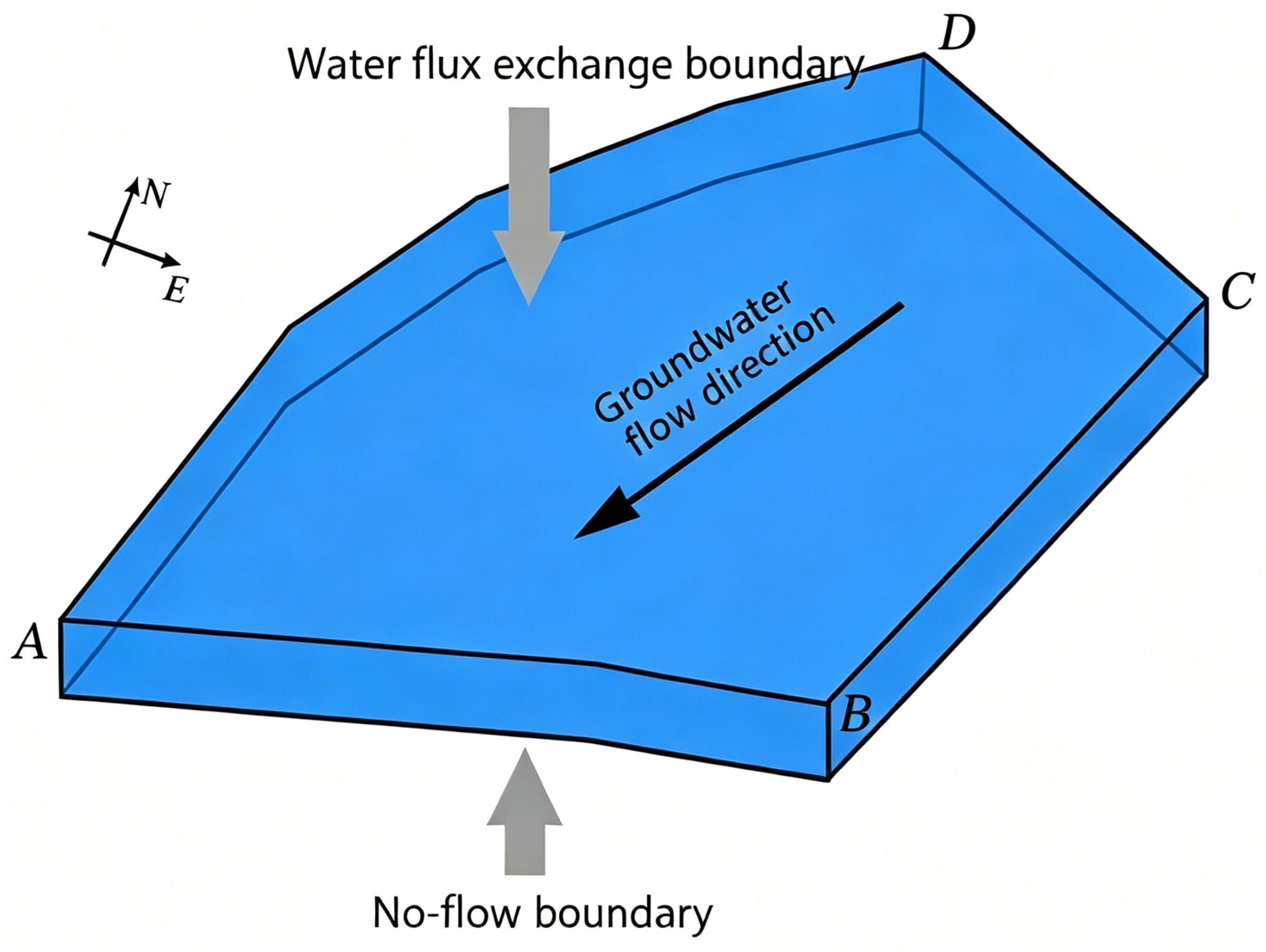
Based on a comprehensive analysis of the site’s geological structure, medium properties, boundary conditions, and recharge–discharge characteristics, the study area is conceptualized as a hydrogeological system with clear constraints. The top of the model represents the water table, which receives infiltration recharge from precipitation and forms a water exchange boundary. The bottom of the model consists of impermeable granite and is set as a no-flux boundary. The eastern side of the model is adjacent to a river and is defined as a constant-head boundary. The remaining lateral boundaries are far from the contaminated core zone, where the impact of contaminant migration is negligible and thus uniformly set as no-flux boundaries. Initial conditions are determined based on background monitoring results, and the initial pressure, saturation, and concentration fields are all set as steady-state fields. A schematic diagram of the conceptual model is shown in Figure 1.

In a multiphase flow system, the aqueous phase, non-aqueous phase, and gas phase migrate simultaneously in porous media under the combined control of pressure gradients, gravity, capillary forces, and viscous drag. Contaminants undergo a series of complex processes including pore entrapment, dissolution into the aqueous phase, diffusion and dispersion, advective migration, and accumulation along impermeable boundaries, exhibiting distinct non-ideal migration behavior. Based on these physical processes, a multiphase flow mathematical model is constructed to fully describe the migration, transformation, and distribution of DNAPLs, laying a foundation for subsequent surrogate model training and inversion calculations [13].

It should be specially noted that in this manuscript, the author(s) used Dola(2.27.11) for the purposes of optimize colors for Figure 1 and Figure 10. The authors have reviewed and edited the output and take full responsibility for the content of this publication.

2.3. Multiphase Flow Numerical Model

In this study, a numerical model for groundwater DNAPL transport is established using mass conservation equations and multiphase Darcy’s law as governing equations. The model comprehensively incorporates component migration, advection, dispersion, molecular diffusion, interphase partitioning, and source–sink effects, enabling a realistic representation of chlorobenzene migration and transformation in subsurface media. The equations include key parameters such as porosity, permeability, saturation, relative permeability, density, viscosity, interfacial tension, and dispersivity, which collectively determine the migration velocity and distribution pattern of contaminants. The relevant parameters of chlorobenzene and water are shown in

Table 1. Parameters of chlorobenzene and water.

Parameter	Chlorobenzene	Water
Density $(\mathrm{kg}\cdot {\mathrm{m}}^{-3})$	1105	1000
Aqueous solubility of chlorobenzene $(\mathrm{mg}\cdot {\mathrm{L}}^{-1})$ (30 °C)	490	--
Chlorobenzene/water interfacial tension $(\mathrm{dyne}\cdot {\mathrm{cm}}^{-1})$	33.02	--
Viscosity $(\mathrm{Pa}\cdot \mathrm{s})$	0.000799	0.001
Residual saturation	0.17	0.24

.

Based on the established conceptual model, a set of mathematical equations is used to describe the transport and diffusion characteristics of DNAPL pollutants, and a numerical simulation model of groundwater DNAPL pollution multiphase flow is established, which includes partial differential equations and definite solution conditions (initial and boundary conditions). The established numerical simulation model is shown below:

$$\left\{\begin{array}{l}{\displaystyle \frac{\partial (\varphi {\tilde{C}}_k{\rho }_k)}{\partial t}}+\overrightarrow{\nabla }\left[{\displaystyle \sum _{l=1}^3{\rho }_k(C_{kl}{\overrightarrow{v}}_l-\varphi S_l{\overrightarrow{\overrightarrow{K}}}_{kl}\overrightarrow{\nabla }{C}_{kl})}\right]=R_k,(x,y,z)\in \mathsf{\Omega },t\ge 0\\ {\overrightarrow{\overrightarrow{K}}}_{kl}={\displaystyle \frac{D_{dkl}}{\tau }}{\delta }_{ij}+{\displaystyle \frac{a_{Tl}}{\varphi S_l}}\left|{\overrightarrow{v}}_l\right|{\delta }_{ij}+{\displaystyle \frac{a_{Ll}-a_{Tl}}{\varphi S_l}}{\displaystyle \frac{v_{li}{v}_{lj}}{\left|{\overrightarrow{v}}_l\right|}},(x,y,z)\in \mathsf{\Omega },t\ge 0\\ {\overrightarrow{v}}_l=-{\displaystyle \frac{k_{rl}\overrightarrow{\overrightarrow{k}}}{{\mu }_l}}(\overrightarrow{\nabla }{P}_l-{\rho }_{l}g\overrightarrow{\nabla }z),(x,y,z)\in \mathsf{\Omega },t\ge 0\end{array}\right.$$

$$\left\{\begin{array}{l}{P}_l(x,y,z,t){|}_{t=0}=P_l^0(x,y,z),(x,y,z)\in \mathsf{\Omega }\\ S_l(x,y,z,t){|}_{t=0}=S_l^0(x,y,z),(x,y,z)\in \mathsf{\Omega }\\ C_{kl}(x,y,z,t){|}_{t=0}=C_{kl}^o(x,y,z),(x,y,z)\in \mathsf{\Omega }\end{array}\right.$$

$$\left\{\begin{array}{l}{P}_l(x,y,z,t){|}_{{\mathsf{\Gamma }}_1}=f_l^1(x,y,z,t),(x,y,z)\in {\mathsf{\Gamma }}_1,t\ge 0\\ {\displaystyle \frac{\partial P_l}{\partial n}}{|}_{{\mathsf{\Gamma }}_2}=0,(x,y,z)\in {\mathsf{\Gamma }}_2,t\ge 0\\ C_{kl}{|}_{{\mathsf{\Gamma }}_1}={\phi }_{kl}^1(x,y,z,t),(x,y,z)\in {\mathsf{\Gamma }}_1,t\ge 0\\ {\displaystyle \frac{\partial C_{kl}}{\partial n}}{{\displaystyle |}}_{{\mathsf{\Gamma }}_2}=0,(x,y,z)\in {\mathsf{\Gamma }}_2,t\ge 0\end{array}\right.$$

In partial differential equations, $k$ is the number of components; $l$ is the number of phases; $\varphi$ is the porosity; ${\tilde{C}}_k$ is the total concentration of component $k$; ${\rho }_k$ is the density of component $k$; $C_{kl}$ is the concentration of component $k$ in phase $l$. Denoting the Darcy flow velocity of phase $l$ as ${\overrightarrow{v}}_l$, $k_{rl}$ is the relative permeability of phase $l$, and $\overrightarrow{\overrightarrow{k}}$ is the inherent (intrinsic) permeability tensor of the porous medium. The saturation of phase $l$ is $S_l$, and the dispersion coefficient tensor representing component $k$ in phase $l$ is ${\overrightarrow{\overrightarrow{K}}}_{kl}$. $R_k$ is the source and sink term of component $k$. The molecular diffusion coefficient is denoted as $D_{dkl}$; the Kronecker delta tensor is denoted as ${\delta }_{ij}$, which serves as tensor index notation in the dispersion tensor expression, with ${\delta }_{ij}$ = 1 when i = j and ${\delta }_{ij}$ = 0 when i ≠ j; the distortion coefficient is denoted as $\tau$. $a_{Tl},a_{Ll}$ are the transverse and longitudinal dispersions of phase $l$. $v_{lj},v_{li}$ are the seepage partial velocities of phase $l$ in the $j$ and $i$ directions, respectively. ${\mu }_l$ is the viscosity of the phase $l$; $z$ is the vertical distance; $P_l$ is the pressure of phase $l$; $g$ is the acceleration of gravity; and ${\rho }_l$ is the density of phase $l$.

In initial conditions, $P(x,y,z,t){|}_{t=0}$ represents the initial pressure distribution in the simulation area; $S_l(x,y,z,t){|}_{t=0}$ is the initial saturation of the phase; $C_{kl}(x,y,z,t){|}_{t=0}$ is the initial concentration of component $k$ in phase $l$; $P^0(x,y,z)$, $S_l^0(x,y,z)$, and $C_{kl}^0(x,y,z)$ are the known functions in the simulation area.

In the boundary conditions, $f_1$ is the known function on boundary ${\mathsf{\Gamma }}_1$; $n$ is the direction of the outer normal of the outer boundary; $f_2$ is the known function on boundary ${\mathsf{\Gamma }}_2$. The closed boundary condition is the simplest form of the known flow boundary, and its flow is 0. $C_{kl}(x,y,z,t){|}_{{\mathsf{\Gamma }}_1}$ is the concentration of component $k$ in phase $l$.

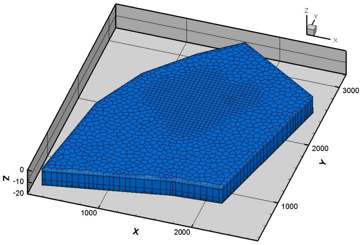
Numerical discretization uses the finite difference method, with refined grids in key zones to improve accuracy, and adaptive time stepping to ensure stability. The spatial discretization map of the study area is shown in Figure 2. Model solution is implemented using mature multiphase flow software, outputting key variables such as concentration, pressure, and saturation at any location and time, providing sufficient and reliable samples for surrogate training [14].

3. Monitoring Data Denoising and Sample Generation

3.1. Adaptive Wavelet Threshold Denoising

Groundwater dynamic monitoring data inevitably introduce environmental noise and instrumental errors during collection and transmission, which directly distort the concentration response relationship and reduce inversion accuracy [15]. Traditional wavelet hard threshold functions exhibit discontinuities at threshold points, easily causing oscillations in reconstructed signals, while soft threshold functions introduce systematic deviations that weaken signal details. To address these problems, an adaptive fusion coefficient is introduced in this study to weight and combine soft and hard thresholds, constructing a continuously differentiable adaptive threshold function with reduced deviation. The fusion coefficient automatically adjusts according to the degree of signal mutation, leaning toward the soft threshold in smooth segments to improve smoothness and toward the hard threshold in mutation segments to preserve details, making the denoising process more adaptive [16].

Furthermore, particle swarm optimization is introduced into the wavelet domain to automatically search for the optimal threshold by minimizing root mean square error (RMSE), replacing fixed threshold strategies [17]. The algorithm iteratively optimizes thresholds matched to real data characteristics. Hypothetical cases show that the proposed method achieves a higher signal to noise ratio (SNR) and lower RMSE than traditional methods under various noise intensities [18], effectively removing noise while retaining true concentration variations, providing high-quality data for subsequent inversion. The comparison of denoising performance of different threshold functions is shown in

Table 2. Comparison of denoising performance of different threshold functions.

Noise Intensity	Hard Threshold Function		Soft Threshold Function		Adaptive Threshold Function		PSO-Optimized Threshold
	RMSE	SNR (db)	RMSE	SNR (db)	RMSE	SNR (db)	RMSE	SNR (db)
0.05	0.356	29.47	0.311	36.61	0.165	39.25	0.119	42.56
0.10	0.397	27.81	0.315	32.76	0.197	37.49	0.125	39.43
0.15	0.412	26.98	0.326	30.89	0.202	35.24	0.143	37.38
0.20	0.429	23.35	0.371	28.05	0.205	33.18	0.154	35.64

.

Through the verification of the hypothetical example above, it can be seen that the particle swarm optimization adaptive wavelet threshold denoising method can not only effectively eliminate the noise of monitoring data, but also significantly improve the denoising performance compared to traditional denoising methods. Therefore, this method will be applied to the case study in this article.

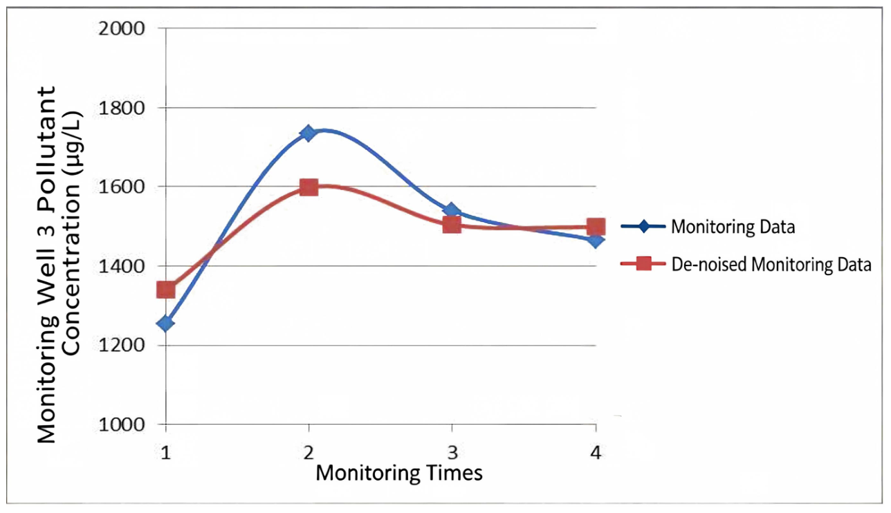
In this study, three dynamic monitoring wells were set up in a chemical pollution site, and they were monitored once a month to obtain corresponding dynamic monitoring data of water level and concentration. The whole monitoring period lasted for 12 months. For each monitoring well, 12 raw monthly concentration observations were collected, yielding 36 total raw observations across the three wells. Considering that monthly pollutant concentration data are susceptible to short-term random fluctuations caused by hydrogeological disturbances, abnormal monthly records were firstly filtered out. Quarterly averaged concentrations were then computed, and 4 quarterly average time series observations per well were finally obtained, with 12 aggregated observations in total for the three monitoring wells, and the particle swarm optimization adaptive wavelet threshold denoising method was applied to denoise the monitoring data.

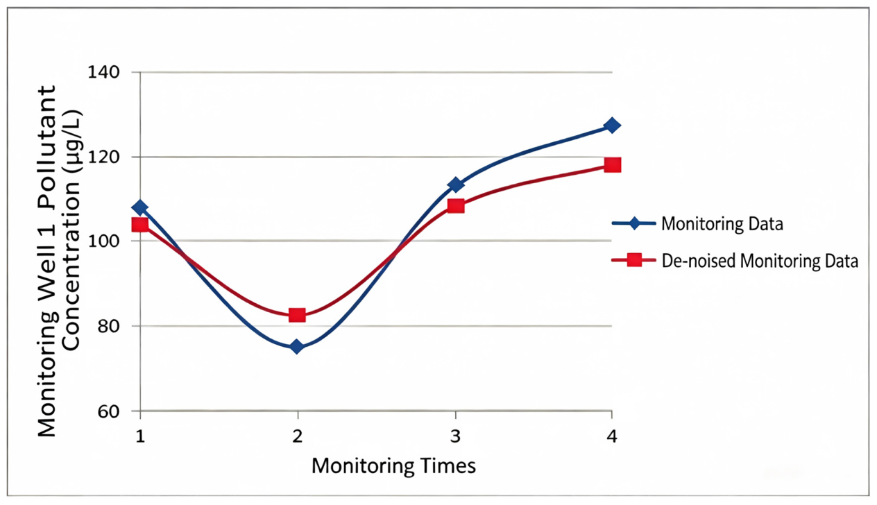
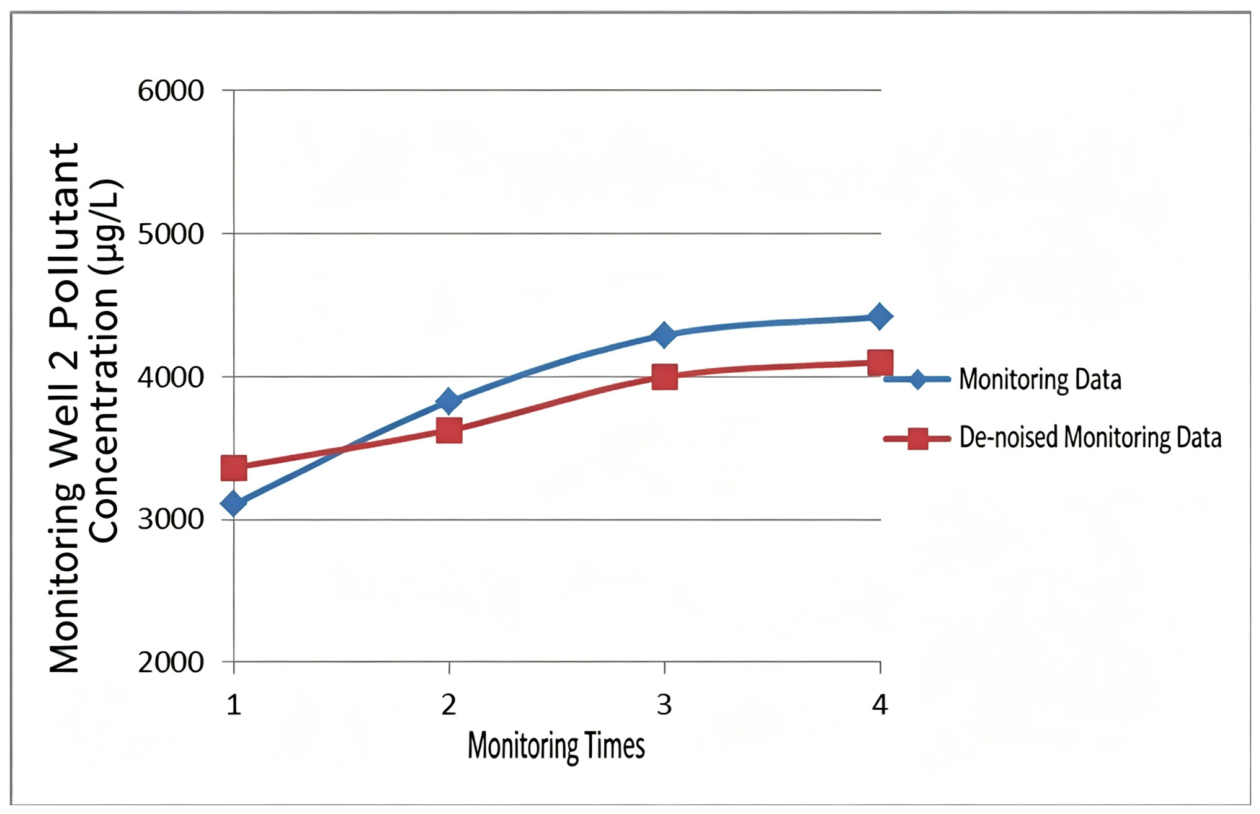
The denoising results of monitoring wells 1, 2, and 3 are shown in Figure 3, Figure 4, and Figure 5, respectively. The relevant parameters of the particle swarm optimization algorithm in the threshold optimization process are shown in

Table 3. Parameter values of PSO in the threshold optimization process.

Parameter	Value
Population size	20
Maximum number of iterations	100
Personal cognitive acceleration coefficient c1	1.5
Social cognitive acceleration coefficient c2	1.7

.

3.2. Parameter Sensitivity Analysis

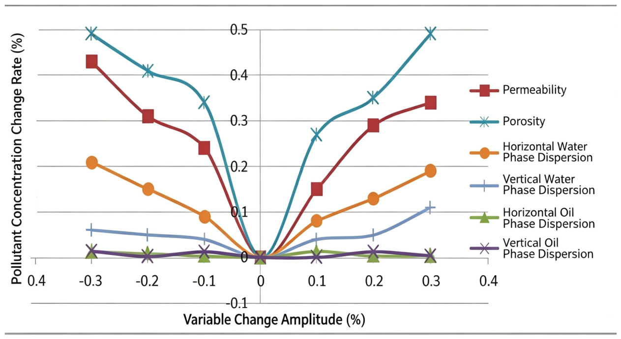
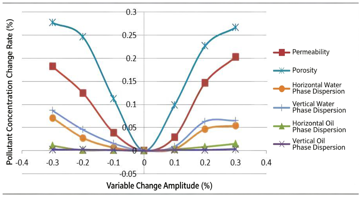
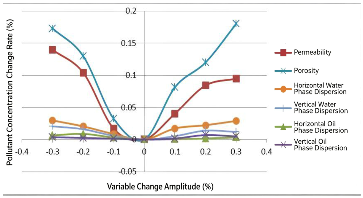
Not all parameters in a multiphase flow model exert the same influence on concentration output. To reduce input dimensionality and improve surrogate model efficiency and accuracy, a local sensitivity analysis method is adopted in this study to evaluate the influence of parameter variations on output concentration one by one. While keeping other parameters constant, the target parameter is varied within a reasonable range, and the change rate of the concentration response is calculated to measure parameter sensitivity [19].

Systematic calculations indicate that porosity, permeability, longitudinal water-phase dispersivity, and transverse water-phase dispersivity most significantly affect concentrations at monitoring points, while parameters such as oil-phase dispersivity show low sensitivity. Therefore, these four highly sensitive parameters, together with the horizontal and vertical coordinates of the pollution source, release duration, and total leakage volume, are collectively used as identifiable variables, while other parameters are set as constants during inversion. This greatly simplifies the input structure while ensuring the model’s expressive capability. The sensitivity analysis results for the three monitoring wells are shown in Figure 6, Figure 7 and Figure 8.

3.3. Latin Hypercube Sampling and Dataset Construction

To ensure uniform and representative coverage within the feasible domain, Latin hypercube sampling is used to generate input samples [20,21]. As a stratified sampling technique, it achieves efficient coverage of high-dimensional space with a relatively small sample size, avoiding clustering and blank areas common in traditional random sampling. Sampling ranges are comprehensively determined based on site conditions and expert experience, with source coordinates, release duration, leakage volume, and hydrogeological parameters sampled within reasonable intervals.

The generated input samples are individually input into the multiphase flow numerical model for forward simulation to obtain the corresponding concentration outputs at monitoring wells, forming input–output sample pairs. A total of 120 groups of samples were generated by Latin hypercube sampling in this study. The whole dataset was randomly divided into a training set and an independent validation set according to a partition ratio of 5:1. Among them, 100 samples were used for model training, and the remaining 20 samples served as the held-out independent validation set, which was not involved in the training process and was used to evaluate the generalization performance of the surrogate model. Only partial representative sample entries are listed in

Table 4. Training samples.

Number	Input Data								Output Data
	M1	M2	M3	M4	M5	M6	M7	M8	W1	W2	W3
1	1241.88	2463.57	4476	2.55	0.2502	3967.65	49.44	11.36	72.75	4359.86	1520.82
2	1354.68	2406.09	4061	1.84	0.2498	3810.62	46.31	9.99	58.88	3911.17	1709.76
3	1906.65	2252.55	3109	3.06	0.2532	3940.13	45.77	10.01	59.45	2044.59	2493.96
4	1497.14	2133.95	4364	2.47	0.2609	4001.87	52.03	10.15	30.69	11,072.06	3332.61
5	2162.17	2389.08	3616	1.32	0.2414	4103.99	55.32	11.67	83.46	6954.02	8281.19
…	…	…	…	…	…	…	…	…	…	…	…
96	1233.85	2465.76	3238	2.18	0.2508	3837.76	50.64	11.44	105.98	1972.23	2726.65
97	1540.96	2489.02	4910	3.16	0.2379	3913.33	48.17	10.51	113.63	5521.36	3185.27
98	2147.61	2271.96	4102	4.03	0.2499	4180.09	45.08	12.64	42.69	8282.69	1049.02
99	1809.05	2366.28	4562	3.43	0.2537	3765.74	46.94	12.28	97.42	7211.23	2550.94
100	1932.41	2175.78	4788	2.25	0.2477	4049.98	51.16	11.32	134.37	5891.87	1999.43

and

Table 5. Verification samples.

Number	Input data								Output data
	M1	M2	M3	M4	M5	M6	M7	M8	W1	W2	W3
1	1299.82	2434.98	3059	3.27	0.2555	3907.51	50.82	11.54	95.24	7722.69	1283.81
2	2125.42	2369.86	3525	2.10	0.2610	3885.25	49.58	12.04	52.15	4509.54	2996.63
3	1823.43	2263.93	4359	4.46	0.2351	4059.95	51.39	12.11	61.24	4972.47	1565.68
4	1420.73	2421.41	4917	2.03	0.2426	4129.11	47.63	10.01	74.21	2236.74	3603.26
5	1752.46	2055.37	4507	3.84	0.2394	4257.14	42.94	11.65	104.19	1817.04	3018.97
…	…	…	…	…	…	…	…	…	…	…	…
16	2143.74	2129.93	3889	4.34	0.2735	3902.27	57.95	10.87	78.69	14,649.29	8418.83
17	2062.20	2422.46	3755	3.15	0.2575	3799.05	49.72	10.98	128.68	8963.53	2869.96
18	1566.91	2049.06	3474	2.37	0.2438	3694.10	50.19	11.42	123.36	4062.08	2501.14
19	1392.73	2358.31	4670	4.66	0.2360	4097.52	46.84	12.93	139.96	2395.45	1608.32
20	2109.23	2231.14	4775	3.65	0.2653	3936.76	53.06	9.74	84.91	3066.19	3352.34

due to page length constraints. The training samples are shown in Table 4, and the validation samples are shown in Table 5.

4. DCNN Surrogate Model Construction and Validation

4.1. Establishment of DCNN Surrogate Model

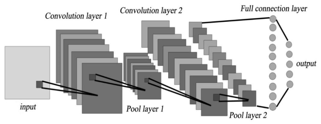
The deep convolutional neural network method (DCNN) is a convolutional neural network with a multi-hidden layer structure, which belongs to one of the deep learning algorithms. This method is mainly composed of a convolutional layer, pooling layer, and fully connected layer, as shown in Figure 9. It is essentially a multi-layer perceptron. Through weight sharing and local connection, the number of weights is effectively reduced, making the network easy to optimize and reducing the risk of overfitting.

Take the horizontal coordinate of the pollution source, the vertical coordinate of the pollution source, the migration and transformation time of the pollutant, the leakage of the pollutant, the porosity, the permeability, the vertical water phase dispersion, and the horizontal water dispersion as inputs, which are represented by M1–M8 in sequence. Take the pollutant concentrations at the bottom of the aquifer at the end of the three monitoring wells as the outputs, which are represented by W1 to W3 in sequence. Apply the deep convolutional neural network method to establish the surrogate model of the multiphase flow numerical simulation model.

Firstly, apply the Latin hypercube sampling method to sample the above eight variables (M1–M8) within the feasible range, input the extracted 100 sets of data into the multiphase flow numerical simulation model for calculation, and obtain 100 sets of input–output training samples for training the surrogate model. Then, use the same method to obtain 20 sets of input–output verification samples for verifying the surrogate model. Secondly, normalize the training samples and verification samples. Finally, use the MATLAB platform to train and verify the deep convolutional neural network model with the training samples and verification samples, and the deep convolutional neural network surrogate model is established. The steps of establishment are as follows:

(1)

Forward Conduction Process

In the forward conduction stage of training samples, a convolutional kernel suitable for the identification of groundwater pollution source is constructed and a reasonable hidden layer structure is designed. Through the alternate operation of convolution and pooling, feature extraction is performed on the original data. After the cumulative transformation of the multi-layer, it is mapped to a high-level abstract feature, and finally the result is output through the inner product calculation of the fully connected layer.

The deep convolutional neural network surrogate model established in this research contains 8 hidden layers. The volume base layer uses the ReLU activation function to continuously map the sample data to the high-dimensional space, as well as to learn and train the feature information in the sample data. Then, the extracted feature information is sampled for dimensionality reduction through the pooling layer, which reduces the amount of calculation and improves the calculation efficiency of the surrogate model. In the structure of the surrogate model, each convolutional layer and each pooling layer are alternately arranged to accurately and efficiently extract the feature information from the training samples.

Since the output of the surrogate model is the concentration value of the pollutant, it is a regression problem, so the value of the last layer of neurons of the deep convolutional neural network is used as the output value.

(2)

Back Propagation Process

Compare the output value obtained by the forward conduction with the target value. If the error is too large, use gradient descent to find the error of the previous layer according to the error of the output layer, until it reaches the input layer, and constantly adjust the weight and bias during this period. Repeat this process until the accuracy requirements are met.

4.2. Surrogate Training and Accuracy Comparison

After sample normalization, surrogate models are constructed using Kriging, support vector regression [22], and deep convolutional neural networks, and accuracy evaluation is performed using independent validation samples. To guarantee a fair comparison among different surrogate model architectures, Kriging and SVR are also tuned within their commonly adopted parameter search ranges. The parameter search space covers typical configuration options for Kriging (covariance kernel types and related kernel parameters) and SVR (kernel function, penalty coefficient, and kernel-specific parameters). An identical independent validation dataset is used as the objective metric, and the configuration achieving the best validation set prediction performance is selected as the final Kriging and SVR models. All three models (Kriging, SVR, and DCNN) are trained and validated on exactly the same training validation dataset partition, eliminating the performance bias induced by unequal parameter tuning efforts among different algorithms. Evaluation metrics include maximum relative error, mean relative error, root mean square error, and coefficient of determination. Comparative results show that shallow learning methods such as Kriging and support vector regression exhibit clear accuracy bottlenecks when processing complex multiphase flow mappings, with noticeable deviations between fitting curves and numerical model outputs. In contrast, the predicted outputs of the DCNN surrogate model almost completely coincide with numerical simulation results, and all indicators are significantly superior. The evaluation results are shown in

Table 6. Accuracy evaluation index values of different surrogate models.

Surrogate Model	KRG	SVR	DCNN
Maximum relative error (%)	8.751	7.133	4.614
MRE (%)	5.786	4.654	2.109
RMSE	12.585	9.061	5.103
R2	0.775	0.762	0.998

.

The maximum relative error of the DCNN surrogate model is controlled within 5%, the mean relative error is less than 2.2%, and the coefficient of determination is higher than 0.99, far exceeding the Kriging and SVR models. This indicates that deep learning can effectively capture the complex nonlinear mapping relationships within multiphase flow systems, making it suitable for embedding into iterative inversion frameworks as a high-precision and high-speed surrogate model.

5. Source Inversion Optimization Model and Hybrid Algorithm

5.1. Optimization Model Establishment

In this study on the source identification of DNAPL contamination in groundwater, two optimization models were established for identifying pollution source characteristics and simulation model parameters. The objective function of both models was defined to minimize the fitting error between the simulated and measured contaminant concentrations at monitoring wells.

For the identification of pollution source characteristics, the decision variables of the optimization model included the longitudinal coordinate, transverse coordinate, migration and transformation duration of contaminants, and leakage rate of the pollution source, while the parameters of the simulation model were set as constants. For the identification of simulation model parameters, the decision variables consisted of porosity, permeability, transverse aqueous dispersion, and longitudinal aqueous dispersion, and the pollution source characteristics were kept constant. When simultaneously identifying pollution source characteristics and simulation model parameters, all of the aforementioned variables were adopted as decision variables.

The established surrogate model based on deep convolutional neural network (DCNN) was embedded into the optimization model as an equality constraint. Combined with other constraint conditions, a nonlinear programming optimization model was further constructed for the source identification of DNAPL contamination in groundwater.

The nonlinear programming optimization model for the source identification of groundwater DNAPL contamination is composed of the aforementioned objective function and constraint conditions.

The objective function is expressed as:

$$\min \left[{\displaystyle \sum _{t=1}^4{\displaystyle \sum _{k=1}^3{\left(C_{k,t}-{\tilde{C}}_{k,t}\right)}^2}}\right]$$

In the formula, $C_{k,t}$ is the actual monitoring value of the pollutant concentration in the k-th monitoring well of the t-th monitoring, and ${\tilde{C}}_{k,t}$ is the corresponding simulated calculated value.

The constraints are expressed as follows:

(1) Constraints on the law of solute transport in groundwater (surrogate model of deep convolutional neural network):

$$\tilde{C}=f\left(s,p\right)$$

Here, the simulated calculated concentration vector of pollutants is denoted as $\tilde{C}$; in this study, it is the output of the deep convolutional neural network surrogate model. The parameter vector of the simulation model is denoted as $p$. The pollution source feature vector is denoted as $s$.

(2) Constraints representing the characteristics of pollution sources:

Lateral coordinates: $X^L\le X_i\le X^U$.

Longitudinal coordinates: $Y^L\le Y_i\le Y^U$.

Migration conversion duration: $T^L\le T_i\le T^U$.

Leakage: $M^L\le M_i\le M^U$.

(3) Constraints representing simulation model parameters:

Porosity: $n^L\le n_i\le n^U$.

Permeability: $k^L\le k_i\le k^U$.

Longitudinal aqueous dispersion: ${{\alpha }_{water,L}}^L\le {\alpha }_{water,L}\le {{\alpha }_{water,L}}^U$.

Transverse aqueous dispersion: ${{\alpha }_{water,T}}^L\le {\alpha }_{water,T}\le {{\alpha }_{water,T}}^U$.

5.2. Hybrid Homotopy-PSO Algorithm

Traditional PSO is sensitive to initial values and prone to becoming trapped in local optima in complex nonlinear problems [23]. Homotopy algorithms possess global path-following capability and can smoothly approach the global optimal solution from any initial point. This study combines the advantages of both to construct a hybrid homotopy-PSO algorithm. By constructing linear homotopy mapping, the original optimization problem is decomposed into a series of progressively transitional sub-problems, evolving from a simple initial problem to the original problem. At each step, PSO is used for local optimization, with the result of the previous step as the initial value of the next step, achieving progressive convergence.

A set of homotopy functions, denoted as $H$, are constructed based on the assumed pollution source characteristics and simulation model parameters of groundwater. Via path tracking, these homotopy equations are transformed into least-squares optimization problems, which are solved stepwise to approach the true values of the source characteristics and model parameters.

The parameter contained in the homotopy function $H$ is defined as the homotopy parameter, denoted by $t$, which increases gradually from 0 to 1. When solving for the assumed source characteristics and model parameters, $t=0$ and the homotopy equation satisfies $H=0$. When targeting the true values to be estimated, $t=1$ and the homotopy equation satisfies $H=1$.

In practical research, linear homotopy is generally adopted:

$$\mathrm{H}\left(\mathrm{X},\mathrm{t}\right)=\mathrm{t}\cdot \mathrm{G}\left(\mathrm{X}\right)+\left(1-\mathrm{t}\right)\cdot \mathrm{F}\left(\mathrm{X}\right)$$

The relationships for $G\left(X\right)$ and $F\left(X\right)$ are expressed as $G\left(X\right)=f\left(X\right)-C_{obs}$, $F\left(X\right)=f\left(X\right)-C_0$, where $X$ denotes the groundwater pollution source characteristics or simulation model parameters; the homotopy parameter t ranges within [0, 1]; and f represents the deep convolutional neural network surrogate model of the multiphase flow numerical model. $C_0$ is the concentration vector at monitoring wells calculated by substituting the initially assigned source characteristics or model parameters into the groundwater multiphase flow numerical model, and $C_{obs}$ stands for the field observed concentration vector at monitoring wells.

The homotopy parameter $t$ is discretized over the interval [0, 1] to obtain $t_0=0<t_1<\cdots t_i<\cdots <t_N=1$. Since the homotopy function $H$ continuously depends on $t$, a set of equations can be derived as follows:

$$\left\{\begin{array}{c}H\left(X,t_1\right)=f\left(x\right)-\left(t_1\cdot C_{obs}+\left(1-t_1\right)\cdot C_0\right)=0\\ ⋮\\ H\left(X,t_i\right)=f\left(x\right)-\left(t_i\cdot C_{obs}+\left(1-t_i\right)\cdot C_0\right)=0\\ ⋮\\ H\left(X,t_N\right)=f\left(x\right)-\left(t_N\cdot C_{obs}+\left(1-t_N\right)\cdot C_0\right)=0\end{array}\right.$$

If the interval between $t_i$ and $t_{i-1}$ is set sufficiently small, the corresponding solutions $X_i$ and $X_{i-1}$ of the homotopy equations will be very close to each other.

Based on the above principles, the optimization model can be further rewritten as follows:

$$\begin{array}{l}\min \left[{\displaystyle \sum _{t=1}^4{\displaystyle \sum _{k=1}^3{\left(\left(t_i\cdot C_{k,t}+\left(1-t_i\right)\cdot C_{k,t}^0\right)-{\tilde{C}}_{k,t}\right)}^2}}\right],\begin{array}{c}i=1,2,\dots ,N\end{array}\\ s.t.\left\{\begin{array}{c}\tilde{C}=f\left(s,p\right)\\ X^L\le X_i\le X^U\\ Y^L\le Y_i\le Y^U\\ T^L\le T_i\le T^U\\ M^L\le M_i\le M^U\\ n^L\le n_i\le n^U\\ k^L\le k_i\le k^U\\ {{\alpha }_{water,L}}^L\le {\alpha }_{water,L}\le {{\alpha }_{water,L}}^U\\ {{\alpha }_{water,T}}^L\le {\alpha }_{water,T}\le {{\alpha }_{water,T}}^U\end{array}\right.\end{array}$$

Independent of initial value selection, this algorithm effectively escapes local optima, and its convergence stability and solution accuracy are significantly better than traditional PSO, making it highly suitable for DNAPL source identification problems characterized by strong ill-posedness and high nonlinearity [24].

5.3. Feedback Correction Iterative Solution Procedure

To mitigate the parameter equifinality effect, two independent simulation–optimization identification schemes were employed to separately calibrate the source terms (pollution source characteristics) and simulation model parameters. For the identification of pollution source characteristics, the relevant source variables were treated as unknowns, and simulation model parameters were set as constants in the numerical model, surrogate model, and optimization model. In the identification of model parameters, conversely, model parameters were defined as variables, while pollution source characteristics remained constant across all three models.

To continuously revise and refine the identified pollution source characteristics and model parameters, a closed-loop iterative framework with feedback correction was established [25]. The two aforementioned simulation–optimization procedures were coupled together, and the identification results from the previous iteration were fed into the calculation of the next iteration. Along with the iterative feedback process, the retrieved source characteristics and model parameters were mutually optimized and gradually improved [26]. Through continuous iteration, the simulated contaminant concentrations at monitoring wells gradually converged to the measured values. The iteration was terminated once the convergence criterion was satisfied. The identification results at the end of iteration were taken as the final approximate values of pollution source characteristics and simulation model parameters.

6. Case Validation and Field Application

6.1. Hypothetical Case Validation

To systematically verify the effectiveness of the method, a hypothetical case consistent with real-site conditions is designed. True values of pollution sources and parameters are preset, and error-free “observation data” are obtained through forward simulation before starting the inversion process. Comparisons are conducted using traditional PSO, hybrid homotopy-PSO, and the hybrid algorithm with feedback iteration. Results show that traditional PSO produces large errors and poor stability; the hybrid algorithm significantly improves accuracy without relying on initial values; after adding feedback iteration, errors are further reduced, and each identification result highly matches the true values. The average relative error drops to 3.72%, and the maximum error is reduced from 12.77% to 4.41%, fully verifying the corrective effect of the iteration mechanism.

6.2. Real Site Computation Process

Validated by hypothetical cases, the deep convolutional neural network (DCNN) was adopted in the case study to construct a surrogate model for the multiphase flow numerical simulation. This surrogate model was embedded into the optimization model for DNAPL contamination source identification in groundwater as an equality constraint. Subsequently, a hybrid homotopy particle swarm optimization algorithm was utilized to solve the optimization model. A feedback correction iteration process was further applied to refine the identification results, enabling continuous updating and mutual optimization of pollution source characteristics and model parameters. Finally, the optimal solutions of the inverse identification were obtained.

A total of ten homotopy functions were constructed in the hybrid algorithm, and each was converted into a corresponding optimization problem with the homotopy parameter t set at an interval of 0.1. The particle swarm optimization algorithm was then adopted to solve these ten optimization problems sequentially. To ensure a gradual optimization process, the identification results obtained from the previous model were used as the initial values for solving the subsequent one. When the homotopy parameter t reached 1, the corresponding optimal solution was taken as the final result for groundwater DNAPL contamination source identification.

The identification results obtained from the hybrid homotopy–particle swarm optimization algorithm were continuously revised and improved via the feedback correction iteration process. The iteration was terminated once the results converged steadily to constant values. The resultant values of pollution source characteristics and simulation model parameters for groundwater DNAPL contamination source identification are presented in

Table 7. Identification results of the actual example.

Iteration Number	Pollution Source Characteristics				Simulation Model Parameters
	Horizontal Coordinate (m)	Vertical Coordinate (m)	Migration and Transformation Duration (d)	Leakage Volume (m3)	Porosity	Permeability (md)	Longitudinal Aqueous Phase Dispersivity (m)	Transverse Aqueous Phase Dispersivity (m)
1	1426.73	2138.15	4508.67	1.28	0.269	4310.47	54.58	10.89
2	1458.02	2124.59	4495.83	1.36	0.2661	4390.28	54.93	11.33
3	1550.42	2147.32	4516.79	1.41	0.2654	4476.79	54.75	11.68
4	1539.17	2152.98	4523.08	1.39	0.2613	4235.11	55.06	12.67
5	1568.56	2165.47	4567.25	1.43	0.2596	4198.17	55.74	12.24
6	1574.08	2173.11	4581.06	1.47	0.2535	4123.44	55.93	11.92
7	1578.31	2178.22	4609.98	1.50	0.2542	4090.12	56.01	11.96
8	1579.39	2179.47	4612.50	1.51	0.2542	4089.82	56.02	11.96

.

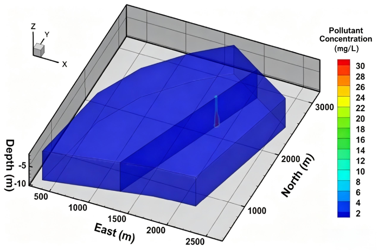
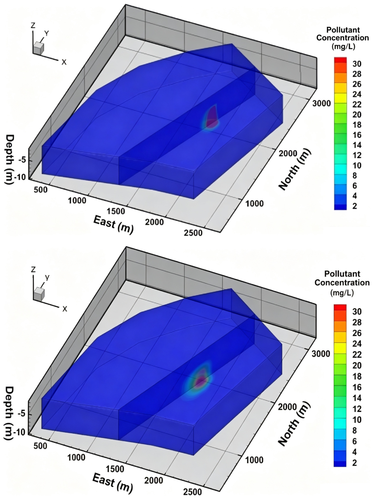
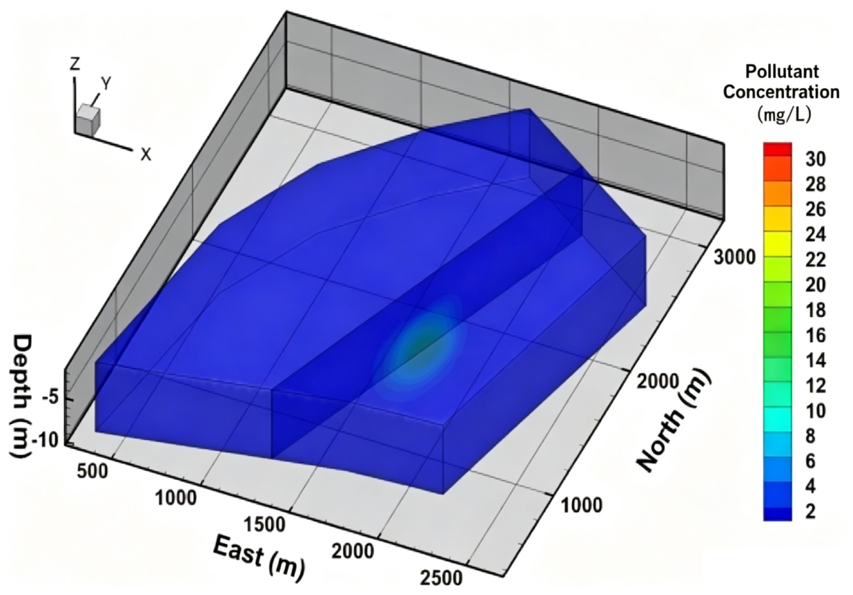
The initially established multiphase flow numerical model for groundwater DNAPL contamination was revised and refined using the identified pollution source characteristics and model parameters. The updated model was then run to simulate the temporal and spatial distribution of DNAPL contaminants in the study area, as illustrated in Figure 10. Accurate localization of pollution sources provides a basis for liability confirmation of polluters. Meanwhile, the simulated spatiotemporal distribution of contaminants offers theoretical support for the design and implementation of groundwater remediation schemes.

7. Conclusions

This work addresses critical bottlenecks in DNAPL groundwater source inversion and delivers clear innovations in methodology, algorithm, and practical application. This study establishes a complete inversion framework integrating adaptive denoising, multiphase flow numerical modeling, DCNN surrogate modeling, hybrid homotopy-PSO, and feedback correction iteration to address key challenges in groundwater DNAPL pollution source inversion, including ill-posedness, equifinality, high computational cost, and algorithmic premature convergence. Based on theoretical derivation, hypothetical cases, and real-site applications, the main conclusions are as follows.

(1)

Under the sample and simulation conditions adopted in this study, this study adopts the deep convolutional neural network to construct a surrogate model for the simulation model. Compared with the surrogate models constructed by shallow learning methods including Kriging and support vector regression, the DCNN surrogate model achieves relatively high accuracy. Its maximum relative error is 4.614%, average relative error is 2.109%, and root mean square error (RMSE) is 5.103, all of which are the lowest among the three methods. Meanwhile, the coefficient of determination reaches 0.998, the highest value of the three approaches. The DCNN method shows good potential to effectively improve the approximation capability of the surrogate model to the original numerical model.

(2)

A hybrid homotopy–particle swarm optimization algorithm was developed by combining the homotopy method and particle swarm optimization (PSO). Its applicability was analyzed, and the algorithm was further applied to the case study of groundwater DNAPL contamination source identification. The results show that compared with the standard PSO, the maximum relative error decreased from 12.77% to 9.69%, and the average relative error dropped from 7.62% to 5.96%. The proposed hybrid algorithm exhibits obvious improvements in identification accuracy. It can help to effectively reduce the initial value dependence of traditional heuristic algorithms and facilitates efficient searching for the global optimal solution.

(3)

To avoid the parameter equifinality effect, we proposed a strategy to separately identify pollution source characteristics and simulation model parameters. These two independent identification procedures were coupled to form a closed-loop iteration with feedback correction for refining the retrieved results. The results reveal that compared with the simultaneous identification scheme, the maximum relative error decreased from 9.69% to 4.41% and the average relative error dropped from 5.96% to 3.72% after iterative feedback correction. This iterative framework is capable of enabling the continuous updating of source characteristics and model parameters, and can substantially improve the overall identification accuracy for the investigated site under given assumptions.

8. Limitations and Future Work

It should be noted that the performance of the proposed framework is subject to several inherent limitations and sources of uncertainty. First, all training and validation samples for the DCNN surrogate are generated from multiphase numerical simulations under simplified aquifer assumptions; real-world aquifers usually contain complex spatial heterogeneity which is not fully represented in the current model, which may bring prediction bias when extended to highly heterogeneous sites. Additionally, the surrogate model generalization capacity is constrained by the Latin hypercube sampling range and sample size. Prediction reliability may decrease when input parameters go beyond the sampled feasible parameter domain.

In future research, more field monitoring datasets will be incorporated to further constrain inversion results. Stratified k-fold cross-validation will be adopted for more robust assessment of surrogate model generalization. Aquifer heterogeneity will be better represented within the numerical model, and quantitative uncertainty analysis will be introduced to provide confidence intervals for inverted source and aquifer parameters.

References

1. Gorelick, S.M.; Evans, B.; Remson, I. Identifying source of groundwater pollution: An optimization approach. Water Resour. Res. 1983, 19, 779–790. [Google Scholar] [CrossRef] [Scilit]
2. Atmadja, J.; Bagtzoglou, A.C. State of the art report on mathematical methods for groundwater pollution source identification. Environ. Forensics 2001, 2, 205–214. [Google Scholar] [CrossRef] [Scilit]
3. Tikhonov, A.N.; Arsenin, V.Y. Solution of Ill-Posed Problem. Math. Comput. 1978, 32, 491. [Google Scholar] [CrossRef] [Scilit]
4. Keller, J.B. Inverse problems. Am. Math. Mon. 1976, 83, 107–118. [Google Scholar] [CrossRef] [Scilit]
5. Queipo, N.V.; Haftka, R.T.; Shyy, W.; Goel, T.; Vaidyanathan, R.; Tucker, P.K. Surrogate-based analysis and optimization. Prog. Aerosp. Sci. 2005, 41, 1–28. [Google Scholar] [CrossRef] [Scilit]
6. Donoho, D.L.; Johnstone, J.M. Ideal spatial adaptation by wavelet shrinkage. Biometrika 1994, 81, 425–455. [Google Scholar] [CrossRef] [Scilit]
7. Lu, J.Y.; Lin, H.; Ye, D.; Zhang, Y. A New Wavelet Threshold Function and Denoising Application. Math. Probl. Eng. 2016, 2016, 1–8. [Google Scholar] [CrossRef] [Scilit]
8. LeCun, Y.; Bottou, L.; Bengio, Y.; Haffner, P. Gradient-based learning applied to document recognition. Proc. IEEE 1998, 86, 2278–2324. [Google Scholar] [CrossRef] [Scilit]
9. Rui, X.F. Opinions on frontier scientific issues in hydrology. Adv. Sci. Technol. Water Resour. 2015, 35, 95–102. [Google Scholar]
10. Hou, Z.Y.; Lu, W.X. Comparative Study of Surrogate Models for Groundwater Contamination Source Identification at DNAPL-contaminated Sites. Hydrogeol. J. 2018, 203, 28–37. [Google Scholar] [CrossRef] [Scilit]
11. Sciortino, A.; Harmon, T.C.; Yeh, W.W. Inverse modeling for locating dense nonaqueous pools in groundwater under steady flow conditions. Water Resour. Res. 2000, 36, 1723–1735. [Google Scholar] [CrossRef] [Scilit]
12. Xin, X.; Lu, W.X.; Luo, J.N. Surrogate model for multiphase flow numerical simulation of DNAPL-contaminated aquifers. J. Jilin Univ. (Earth Sci. Ed.) 2011, 41, 855–860. [Google Scholar]
13. Li, G.S.; Tan, Y.J.; Wang, X.Q. Inverse problem method for determining groundwater pollution source intensity. Appl. Math. 2005, 18, 92–98. [Google Scholar]
14. Luo, J.N.; Lu, W.X. Sobol’ sensitivity analysis of NAPL remediation processes. Comput. Geosci. 2014, 67, 110–116. [Google Scholar] [CrossRef] [Scilit]
15. Datta, B.; Chakrabarty, D.; Dhar, A. Simultaneous identification of unknown groundwater pollution sources and estimation of aquifer parameters. J. Hydrol. 2009, 376, 48–57. [Google Scholar] [CrossRef] [Scilit]
16. Zhou, J.; Xiang, B.P.; Ni, L.; Ai, P. Research on a novel wavelet threshold denoising algorithm. Mach. Des. Res. 2017, 33, 1–5. [Google Scholar]
17. Kennedy, J.; Eberhart, R. Particle swarm optimization. In Proceedings of the IEEE International Conference on Neural Networks, Perth, Australia, 27 November–1 December 1995. [Google Scholar]
18. Ma, Y.J. Research on Solving Methods for Several Types of Ill-Posed Mathematical Physical Inverse Problems. Ph.D. Thesis, Lanzhou University, Lanzhou, China, 2012. [Google Scholar]
19. Simpson, T.W.; Mauery, T.M.; Korte, J.J.; Mistree, F. Kriging models for global approximation in simulation-based multidisciplinary design optimization. AIAA J. 2001, 39, 2233–2241. [Google Scholar] [CrossRef] [Scilit]
20. McKay, M.D.; Beckman, R.J.; Conover, W.J. A comparison of three methods for selecting values of input variables in the analysis of output from a computer code. Technometrics 1979, 21, 239–245. [Google Scholar] [CrossRef] [Scilit]
21. Helton, J.C.; Davis, F.J. Latin hypercube sampling and the propagation of uncertainty in analyses of complex systems. Reliab. Eng. Syst. Saf. 2003, 81, 23–69. [Google Scholar] [CrossRef] [Scilit]
22. Vapnik, V.N. An overview of statistical learning theory. IEEE Trans. Neural Netw. 1999, 10, 988–999. [Google Scholar] [CrossRef] [Scilit]
23. Krohling, R.A.; Coelho, L.D. Coevolutionary particle swarm optimization using Gaussian distribution for solving constrained optimization problems. IEEE Trans. Syst. Man. Cybern. Part B-Cybern. 2006, 36, 1407–1416. [Google Scholar] [CrossRef] [Scilit]
24. Miao, T.; Guo, J.; Li, G.; Huang, H. Inversion-based identification of DNAPLs-contaminated groundwater based on surrogate model of deep convolutional neural network. Water Supply 2023, 23, 129–143. [Google Scholar] [CrossRef] [Scilit]
25. Hou, Z.Y. Uncertainty Analysis of Remediation Optimization for DNAPL-Contaminated Aquifers Based on Surrogate Models. Master’s Thesis, Jilin University, Changchun, China, 2015. [Google Scholar]
26. Dokou, Z.; Pinder, G.F. Extension and field application of an integrated DNAPL source identification algorithm that utilizes stochastic modeling and a Kalman filter. J. Hydrol. 2011, 398, 277–291. [Google Scholar] [CrossRef] [Scilit]
Figure 1. Schematic diagram of the conceptual model.
Water 18 02185 g001
Figure 2. Spatial discretization grid map of study area.
Water 18 02185 g002
Figure 3. Monitoring data denoising results of observation well 1.
Water 18 02185 g003
Figure 4. Monitoring data denoising results of observation well 2.
Water 18 02185 g004
Figure 5. Monitoring data denoising results of observation well 3.
Water 18 02185 g005
Figure 6. Sensitivity analysis results of well 1.
Water 18 02185 g006
Figure 7. Sensitivity analysis results of well 2.
Water 18 02185 g007
Figure 8. Sensitivity analysis results of well 3.
Water 18 02185 g008
Figure 9. Structure of deep convolutional neural network.
Water 18 02185 g009
Figure 10. Spatial and temporal distribution of pollutant concentration in the actual example.
Water 18 02185 g010aWater 18 02185 g010bWater 18 02185 g010c