Article

Numerical Study of Culvert–Weir Operating Modes Under Steady and Unsteady Hydrographs: Stage Response, Regime Transition and Ventilation State

1
Department of Civil-Industrial Engineering and Architecture, University of Catania, 95123 Catania, Italy
2
Department of Environment, Land and Infrastructure Engineering, Politecnico di Torino, 10129 Turin, Italy
*
Author to whom correspondence should be addressed.
Water 2026, 18(17), 2081; https://doi.org/10.3390/w18172081
Submission received: 20 July 2026 / Revised: 20 August 2026 / Accepted: 21 August 2026 / Published: 24 August 2026

Abstract

Culverts are widely used to provide crossings over small rivers and can strongly influence flood hydraulics by controlling upstream water levels. During high flows, insufficient conveyance may cause pressurization and overtopping, with important implications for flood hazard assessment. Although computational fluid dynamics (CFD) is increasingly applied to investigate these complex hydraulic processes, systematic evaluations of its performance remain limited. This study addresses this gap by validating a three-dimensional CFD model against previously published laboratory experiments for culvert-only, weir-only and combined culvert–weir configurations under both steady (rising and receding discharge sequences) and unsteady flow conditions. Beyond benchmark validation, diagnostic analyses examined inlet region mesh resolution, inflow ramp history and turbulence closure, together with the associated outlet ventilation and attachment mechanisms. The model reproduced upstream water levels with mean absolute relative error (MARE) values ranging from 0.90% to 5.42% and captured the main stage–discharge relationships across the tested configurations. However, the experimentally observed transition from partially full to pressurized flow in the combined culvert–weir configuration was not reproduced consistently. The diagnostic analyses showed that inlet resolution influences entrance losses and post-submergence headwater, inflow history alters outlet attachment and ventilation and turbulence closure affects barrel filling and air-pocket morphology. The results indicate that CFD can reproduce water level and overtopping responses well when carefully configured, while regime transition prediction remains more uncertain because of its sensitivity to ventilation and discharge history effects.

1. Introduction

Culverts are widely used hydraulic structures that convey water beneath roadways, embankments and settlements. Their hydraulic performance depends on geometry, roughness and flow conditions [1].
In urban settlements, hydraulic protection is often constrained by the limited conveyance of culverted drainage systems, because these structures can act as local hydraulic controls that raise headwater when capacity is approached or exceeded [2,3].
Culvert operation is commonly classified as operating under inlet control or outlet control, depending on the section that limits the conveyed flow rate. Under inlet control, discharge is primarily limited by the entrance geometry, whereas under outlet control, discharge is limited by the barrel and downstream conditions, including friction, minor losses and tailwater [1,4]. Culverts may exhibit subcritical, supercritical and pressurized states [5]. In culvert–weir systems, rising headwater can also activate overtopping while flow continues through the barrels, so the hydraulic response depends on the interaction between the two conveyance mechanisms [6]. Transitions between these regimes can cause marked changes in upstream water level and increase flood risk, particularly under increasing discharges [4,7,8,9]. Furthermore, during rapid filling or inadequate ventilation, trapped air pockets may form in closed or partially filled conduits/culverts and amplify pressure fluctuations, complicating hydraulic response beyond steady, single-phase assumptions [10,11,12,13].
Conventional hydraulic analysis relies on empirical equations, such as the Manning and energy equations, alongside 1D models and physical models [14,15,16]. Recent discussions regarding Manning-based 1D models in flood hydraulics further characterize the application of these foundational theories [17]. While these methods are effective for simple conditions, they are limited in capturing complex geometrical features, including junctions, branching and complex layouts [18,19,20,21].
Enhanced 1D methods, such as the Preissmann slot, provide simplified representations of mixed free-surface and pressurized flow [22,23]. Under extreme conditions, such as intense rainfall and urban flooding, 1D approaches can misrepresent inundation extent and depth [18,24,25].
The limitations of traditional methods highlight the need for more detailed tools to better quantify both flow conveyed through the culvert and flow spilled by overtopping, which remains a critical challenge for civil protection. Computational fluid dynamics (CFD) has increasingly been applied to culvert hydraulics using platforms such as FLOW-3D, ANSYS Fluent and OpenFOAM. These models simulate culvert hydraulics by solving the Reynolds-averaged Navier–Stokes equations and commonly employing the volume of fluid (VOF) method to capture free-surface evolution, enabling detailed representation of flow regimes and turbulence [26,27].
For example, ANSYS Fluent has been adopted in studies concerning culverts with blockage, scour and gated flow conditions. Within this context, Zeng et al. [28] used dimensional analysis to develop gated culvert discharge relationships for different flow types. OpenFOAM has also been used in culvert hydraulics, including two-phase CFD simulations under blockage scenarios validated against laboratory velocity measurements [29] and CFD–flume comparisons assessing how streamlined inlet and outlet profiles can reduce head losses and lower headwater for a given discharge [30].
Flow-3D has also been applied to downstream scour and bed form change as functions of bed resistance and diversion, wing wall, and headwall configurations [31]. Related applications have examined velocity- and energy-dissipating culvert ends intended to reduce downstream erosion [32], while RNG-based simulations investigated scour under variable flows, including inlet blockage cases [33]. Other studies quantified how partial inlet blockage altered scour characteristics, with the blockage ratio identified as the dominant control on scour depth [34,35]. Under partial blockage in box culverts, internal obstructions were found to have a limited influence on scour depth, and an empirical relationship was proposed linking blockage ratio with submergence ratio and Froude number [36].
Despite the wide use of CFD models in culvert applications, most previous numerical studies have remained focused on specific mechanisms such as blockage, outlet scour and local protection measures, rather than providing a broader assessment of the suitability of CFD to study culvert hydraulics under both steady and unsteady conditions. As a result, the systematic evaluation of the suitability of CFD to study the hydraulic capacity and regime behavior across boundary conditions, including time-varying headwater response and transitions between flow regimes, has remained limited in the numerical literature.
This represents a significant gap, as professionals interested in applying CFD to real-world projects often lack clear guidance on the selection of the most critical numerical parameters, the conditions under which the model performs reliably, and the mechanisms that are not yet fully captured by numerical methods and may therefore require, where relevant in practical applications, an alternative approach. In this context, the present study uses the published laboratory measurements of Meselhe and Hebert [6] as the experimental benchmark and extends the analysis through three main objectives: (i) benchmark validation of the FLOW-3D model for three configurations (weir-only, culvert-only and combined culvert–weir), with emphasis on water stages and regime transitions; (ii) numerical sensitivity and diagnostic analyses examining inlet region mesh resolution, turbulence closure, surface tension and air entrainment with attention to their influence on headwater response, barrel filling, air-pocket development and local flow behavior; and (iii) investigation of how the experimentally undocumented discharge ramp time between successive flow levels may influence the outlet ventilation state, defined here as the presence or absence of an air region at the outlet, and the resulting flow regime transition.

2. Experimental Benchmark

This study is based on the previously published laboratory data of Meselhe and Hebert [6], which report steady stage–discharge h Q curves and an unsteady state hydrograph for a culvert–weir structure. No new laboratory geometry or additional physical experimental case was introduced in the present study. The dataset is particularly rich as it encompasses a wide variety of hydraulic behaviors. These data provide a controlled benchmark for assessing numerical accuracy in capturing flow regimes and transitions, as they were originally developed for model calibration and validation.
In the following, only the essential information on the experimental setup of Meselhe and Hebert [6] is provided. Additional details on the experimental apparatus, boundary-control procedure and instrumentation as reported in the original study are included in Appendix A for the convenience of interested readers.

2.1. Physical Model

The published experimental benchmark was conducted in a rectangular laboratory flume using three configurations: culvert-only, weir-only and combined culvert–weir. The weir crest was located 154 mm above the flume bed.
The culvert configuration comprised two circular barrels with diameter D = 76.2 mm and lengths L = 0.381 m. The term culvert-only flow denotes the condition in which flow passes exclusively through the culvert barrels, whereas weir-only flow refers to the condition in which discharge occurs exclusively by overtopping the weir. When both mechanisms occur simultaneously, the flow condition is referred to as combined culvert–weir flow.

2.2. Tested Flow Rates and Hydrographs

The experimental setup encompasses several types of operation, including culvert-only flow without overtopping, weir-only flow without the culvert and combined culvert–weir flow with the possibility of overtopping. These configurations are examined under both steady state and unsteady state flow conditions. The steady sequences include both a rising limb of the hydrograph, in which discharge is increased progressively from low to high values, and a receding limb, in which discharge is decreased from higher values back towards low flow as the system drains.
The steady program comprised rising and receding culvert-only sequences, a rising weir-only sequence and rising and receding combined culvert–weir sequences. The corresponding discharge ranges and numbers of experimental values are summarized in Table 1a.
Under unsteady conditions, the combined culvert–weir configuration was tested using a continuous rising-and-receding hydrograph, also summarized in Table 1a.

2.3. Boundary Conditions

Only free-flowing experiments were selected for this study because these are the cases for which the required data are fully reported. In these free-flow cases, the tailwater does not impose downstream control on the culvert–weir response. The experimental inflow and tailwater control procedures are described in Appendix A, while the corresponding numerical boundary conditions are specified in Section 3.2.3.

2.4. Available Data

The published dataset provides water level and discharge records for the steady and unsteady experiments. Details of the experimental instrumentation and measurement procedure are provided in Appendix A.
The data were used to develop h Q curves and to identify regime transitions. For the culvert-only experiments, the rising and receding limbs were performed as two separate steady test series, one ranging from low to high and the other from high to low; as such, these limbs are treated separately in the analysis. In contrast, the culvert–weir experiments were conducted in a single continuous steady sequence from low to peak and back to low and are therefore treated as a single looped h Q curve.
Two possible regimes were considered: partially full and pressurized. Partially full (free-surface) flow occurs when the water depth is below the culvert crown, and the flow is characterized by an internal air region and a distinct air–water interface. Pressurized (full-barrel) flow occurs when the culvert cross-section is completely filled.

3. Numerical Simulation Setup

3.1. FLOW-3D Solver

The numerical simulation setup used FLOW-3D HYDRO 2025 R1 (Flow Science, Inc., Santa Fe, NM, USA)., a 3D CFD solver designed for civil and environmental hydraulics. It solves the incompressible RANS (Reynolds-averaged Navier–Stokes) equations with the VOF (volume of fluid) method to capture free-surface flows. The model uses the FAVOR (fractional area/volume obstacle representation) technique to represent culvert and weir geometries inside a structured mesh without requiring body-fitted grids.
FLOW-3D expresses the conservation equations using the FAVOR fractional open-volume and open-area functions. For the Cartesian coordinates used in the present simulations, with inflow prescribed at the domain boundary rather than through an internal mass source, the incompressible continuity equation reduces to:
x ( u A x ) + y ( v A y ) + z ( w A z ) = 0 ,
and the corresponding momentum equations in the three Cartesian directions are:
u t + 1 V F ( u A x u x + v A y u y + w A z u z ) = 1 ρ p x + G x + f x b x ,
v t + 1 V F (   u A x v x + v A y v y + w A z v z ) = 1 ρ p y + G y + f y b y ,
w t + 1 V F ( u A x w x + v A y w y + w A z w z ) = 1 ρ p z + G z + f z b z ,
where t is time; u , v and w are the velocity components in the x , y and z directions, respectively; ρ is the fluid density; and p is pressure. The FAVOR quantities V F and A x , A y and A z denote the fractional cell volume and fractional face areas open to flow, respectively. G x , G y and G z are body accelerations; f x , f y and f z are viscous accelerations; and b x , b y and b z represent flow losses associated with porous media or baffles.
The benchmark simulations employed the RNG k–ε turbulence model. This closure was selected as the baseline because the investigated flow involves strong shear, acceleration, separation and recirculation, conditions for which RNG k–ε has been successfully applied in previous FLOW-3D studies of complex hydraulic structures, including supercritical bend manhole and vortex drop shaft flows [37,38]. In FLOW-3D, this two-equation closure solves transport equations for the turbulent kinetic energy k T and ε T , its dissipation rate, while retaining the FAVOR area and volume fractions. The turbulent kinetic energy equation is:
k T t + 1 V F (   u A x k T x +   v A y k T y +   w A z k T z ) = P T + G T + D i f f k T ε T ,
The corresponding dissipation rate equation is:
ε T t + 1 V F (   u A x ε T x +   v A y ε T y +   w A z ε T z ) = C D I S 1 ε T k T ( P T + C D I S 3 G T ) + D i f f ε C D I S 2 ε T 2 k T ,
where P T and G T   are the turbulent energy production terms associated with shear and buoyancy, respectively, while D i f f k T and D i f f ε   represent diffusion of turbulent kinetic energy and dissipation. The RNG model uses the FLOW-3D coefficients C D I S 1 , C D I S 2 , C D I S 3 and   C N U , with the turbulent kinematic viscosity evaluated as ν T = C N U k T 2 / ε T .
The simulation further incorporates a surface tension model to represent surface tension forces at the water–air interface. For an interface whose inward surface normally points in the negative z-direction, the z-component of the surface tension force is evaluated as:
S z = σ cos ( θ ) cos ( ϕ ) d y ,
where σ is the surface tension coefficient, θ is the angle of the second principal tangent with respect to the z-axis and ϕ is the angle of the first principal tangent with respect to the y-axis.
An air entrainment model is included to represent the entrainment, transport and release of air within the liquid due to turbulence at the free surface. The model introduces an entrained air concentration C, governed by:
{ t C + u C [ D C C ] = f I N f O U T ρ F L = ρ F L ( C ) f I N = α [ 2 ( ρ k T ρ g n L t 2 σ / L t ) ρ ] 1 / 2 ,     f O U T = f O U T ( C )
where the first relation describes advection and diffusion of entrained air together with source and sink terms, the second describes the variable fluid density and the third quantifies the entrainment rate at the surface. Here, with u = ( u , v , w ) denoting the velocity vector, C is the entrained air concentration and D C is its diffusion coefficient; f I N is the air entrainment source term at the free surface and f O U T is the air release (degassing) sink term expressed as a function of C ; α is the surface of contact where the entrainment can happen; g n is the gravity normal to free surface; and L t is the turbulent mixing length.
The numerical solution is based on the VOF method [39]. The free surface is represented by the fluid fraction F , where F = 0 corresponds to a void region, F = 1 corresponds to water and 0 < F < 1 denotes the free-surface region. The free surface is tracked by the transport equation:
F t + 1 V F [ x ( F A x u ) + y ( F A y v ) + z ( F A z w ) ] = 0 ,
The solver uses a TruVOF scheme, an advanced implementation of the classical VOF method for interface tracking, coupled with the FAVOR method.
The FAVOR method is used for geometric representation. The fractional open volumes and face areas introduced above account for portions of the Cartesian cells blocked by the culvert, weir and channel boundaries and are incorporated directly into the conservation and VOF transport equations.

3.2. Model of the Channel

3.2.1. Geometry

Regarding the channel geometry, the numerical model matched the laboratory flume dimensions exactly. Because the material of the culvert–weir structure was not reported in the experimental study, the numerical model assumed the same material treatment as the flume substrate. For the inlet, two configurations were evaluated. Option 1 applied a standard inlet boundary condition directly at the upstream face (see Section 3.2.3), while Option 2 involved an inlet conditioning system featuring three porous baffles to represent the laboratory diffuser screens and perforated wall.
Ultimately, Option 2 produced no meaningful change in predicted stages compared with Option 1; therefore, the standard inlet boundary was adopted to reduce computational cost.
Similarly, two outlet configurations were tested. Option 1 utilized a standard outlet boundary condition applied at the downstream face, whereas Option 2 incorporated a tail-tank drop box. This box was 0.30 m in length with an invert set 0.15 m below the culvert invert to mimic discharge into the laboratory tail tank. As with the inlet testing, Option 2 resulted in no significant difference in predicted water levels. Consequently, Option 1 was selected to avoid unnecessary run time and ensure computational efficiency.

3.2.2. Mesh

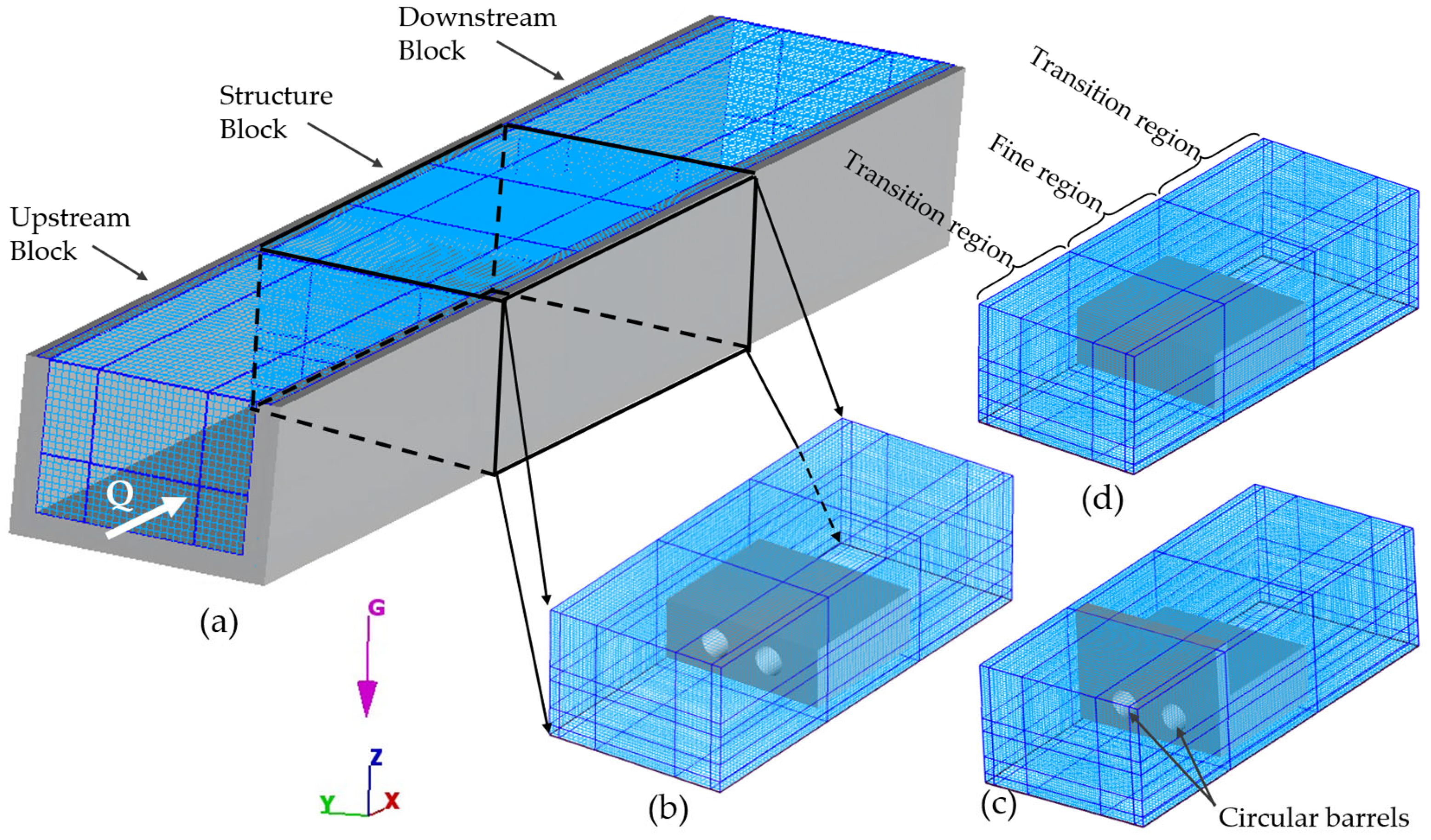
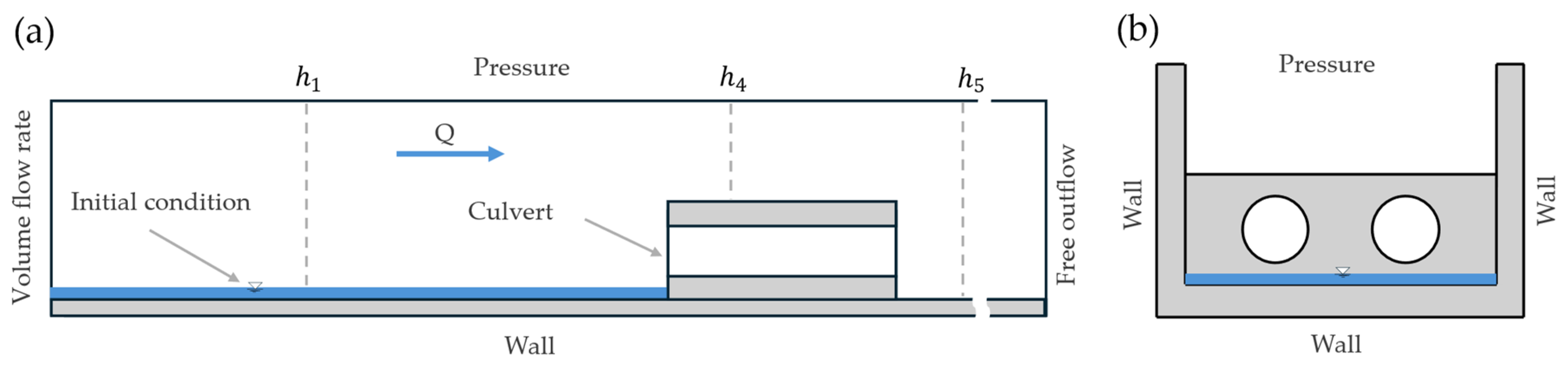
The computational domain was discretized using a non-conforming, block-structured Cartesian mesh. This architecture decouples cell face alignment at block interfaces, permitting localized refinement without global discretization penalties. Continuity of mass and momentum across these interfaces is maintained through inter-block interpolation. The domain comprises three primary blocks: an upstream block (inlet), the central culvert–weir structure block and a downstream block (outlet). The full-flume domain, culvert–weir, culvert-only and weir-only geometries are shown in Figure 1a–d, respectively.
Grid refinement was prioritized in the vicinity of the culvert barrels and weir crest to capture critical flow features. For the benchmark configuration, coarse upstream and downstream reaches utilized a nominal cell size of 28 mm ( 0.37 D , where D = 76.2 mm). Grid spacing was reduced to 0.16 D in the transition zones located between the coarse upstream and downstream reaches and the central refined region and reached 0.09 D in the fine region encompassing the culvert–weir structure.
This discretization strategy aligns with the established literature, and the baseline refinement levels were selected using the simplified mesh design analysis presented in Appendix B. The near-barrel resolution ( 0.09 D ) satisfies the 0.11 D threshold recommended by Liu et al. [40], who evaluated grid sensitivity for flow around cylindrical bridge piers and identified this spacing as necessary to resolve strong local gradients. Furthermore, the mesh refinement exceeds the 0.20 D 0.25 D requirements reported by Park et al. [41] for 3D structures. The vertical resolution is also consistent with the 0.15 H 0.15 H range (where H is wave height) employed by Tang et al. [42] for numerical wave tanks. This multi-block approach ensures high-fidelity resolution in critical regions while minimizing global computational cost.

3.2.3. Boundary Conditions

The side view and front view boundary conditions of the culvert–weir configuration are shown in Figure 2a,b, respectively; the same boundary conditions were used for the culvert-only and weir-only configurations. The adopted boundary conditions prescribe an upstream volume flow rate matching the experimental discharges and hydrograph, implemented as a uniform inflow over the inlet area A , i.e., u x = Q ( t ) / A and with a zero-gradient pressure condition, p / n = 0 . At the top boundary, a pressure boundary is imposed at atmospheric pressure, p = p atm , together with a free-slip condition for tangential velocity, u t / n = 0 . The sidewalls and bed use no-slip wall boundary conditions with a roughness of 0.0015 mm, applying the no-slip velocity condition u = 0 at the wall. The downstream boundary uses a wave outflow condition to allow exit without backpressure, / t + c / n = 0 , where · is any quantity, n is outward-normal coordinate to the boundary and c is the local phase speed of the outgoing wave.

3.2.4. Inflow Implementation and Hardware Characteristics

The steady h Q curves were simulated by reproducing the experimental discharge levels and rising or receding limb sequences reported by Meselhe and Hebert [6] using a quasi-steady step method, in which the inflow was applied as a sequence of constant discharge plateaus connected by short ramps. For each target discharge level   Q i , the inflow was imposed as a linear ramp from Q i 1   to Q i   over a prescribed ramp time Δ t r   ( = t Q i t Q i 1 ) , followed by a constant-discharge plateau of Q i for Δ t p to allow water levels to stabilize before measurement. This sequence was repeated for all reported experimental discharge levels; no additional values were introduced to target particular hydraulic states. In the baseline setup, Δ t p was set to 60 s for all steps as the stabilization plateau and Δ t r   was set to 5 s as the ramp time. For unsteady state conditions, the complete continuous experimental hydrograph was imposed directly, rising from 2 L/s to 30 L/s and subsequently receding to 2 L/s, over a total time of 32.66 min.
The benchmark setup was defined before comparison with the measurements and without calibration or tuning. Geometry, discharge sequences and the unsteady hydrograph, monitoring locations and principal boundary conditions were exactly the same as those adopted in the physical experiments. Fluid properties and wall roughness were selected on the basis of typical literature data. Inlet resolution, turbulence closure, surface-tension and air entrainment settings and ramp history were initially selected from CFD best practices reported in the literature and later varied in additional numerical analyses to provide sensitivity and diagnostic assessments. The computations were performed on a Windows 10 Pro 64-bit operating system using FLOW-3D HYDRO 2025 R1. The processor was an Intel i7-8700K, with 8 physical cores used. Typical production case cell count ranged from approximately 0.5 to 1.8 million cells. Steady runs required a range of ~8 h–15 d 2 h, while the unsteady hydrograph required ~1 d 22 h.

3.2.5. Evaluation Metrics

The benchmark validation was performed by reproducing the experimentally tested forcing and comparing the CFD results with the corresponding published laboratory data. No experimental cases were withheld as an independent validation set; all reproduced cases were used as benchmark comparisons. The evaluated responses depended on the analysis considered. The steady benchmark comparisons focused on upstream headwater at h 1 , barrel filling state, and the associated transition discharge, whereas the unsteady benchmark comparison examined the water level response at h 1 , h 4 and h 5 . The additional numerical analyses evaluated, as applicable, outlet ventilation and attachment, air-pocket extent, inlet flow structure and wall shear stress, as summarized in Table 1b.
For each discharge scenario, simulated water levels ( h CFD ) were extracted at the end of each 60 s constant-discharge plateau, immediately before the following discharge ramp, and compared directly against experimental values ( h exp ) . At this point, the simulated water level had remained essentially constant for more than 30 s, indicating a stable quasi-steady condition; therefore, no additional time averaging was applied. Furthermore, the validation assessed the numerical model’s capacity to capture regime transitions, specifically the discharge threshold at which the culvert shifts from partially full to full-flow conditions.
For the unsteady comparison, the experimental and CFD time series were aligned using elapsed time from the start of the hydrograph, without temporal shifting or distortion; the experimental datasets were digitized from the published laboratory time-series data, with time intervals that might be different from those of the numerical analysis, and no fixed sampling interval was imposed.
Experimental regime changes were identified from the published steady h Q figures using the reported arrows and annotations indicating the transition between partially full and full-barrel flow. Overtopping and regime intervals were identified from the corresponding published unsteady time-series figures and annotations.
For the CFD results, barrel filling and outlet ventilation were classified from the VOF fluid fraction field F   defined in Section 3.1. A barrel was classified as partially full when a free surface remained within the barrel, indicated by a contiguous void region ( F = 0) bounded by interface cells ( 0 < F < 1 ); a full-barrel state was identified when the internal free surface disappeared and the barrel interior was occupied by water ( F = 1). Outlet ventilation was assessed separately: The outlet was classified as ventilated when a void gap ( F = 0) remained at the downstream end of the barrel between the water surface and the culvert crown. An attached/sealed outlet state was identified when the water phase reached the crown at the outlet and this void gap disappeared. Void regions remaining inside the barrel after closure of the outlet gap were classified as trapped air pockets.
Statistical indicators used in the analysis include the root mean squared error [43,44]:
R M S E = 1 N i = 1 N ( h cfd , i h exp , i ) 2 ,
and the mean absolute error [45,46]:
M A E = 1 N i = 1 N h cfd , i h exp , i ,
Furthermore, the coefficient of determination: [47,48]
R 2 = 1 i = 1 N ( h cfd , i     h exp , i ) 2 i = 1 N ( h exp , i     h ¯ exp ) 2 ,
is employed alongside the mean absolute relative error (MARE), defined as: [49]
M A R E   ( % ) = 100 N i = 1 N | h c f d , i h e x p , i h e x p , i | ,
The benchmark validation cases and additional numerical analyses are summarized in Table 1a and Table 1b, respectively.
The processed data supporting the headwater–discharge comparisons, ramp-time and mesh-sensitivity analyses, and statistical metrics are provided in the Supplementary Materials.

3.2.6. Dimensionless Hydraulic Parameters

To characterize the investigated hydraulic conditions independently of dimensional scale, a set of dimensionless indicators was calculated from the experimental and numerical data. At the upstream monitoring section h 1 , the normalized headwater above the culvert inlet invert and the dimensionless total discharge were defined as:
h = h 1 z i n v D ,
Q = Q g D 5 ,
where z i n v is the culvert inlet invert elevation, Q is the total imposed discharge and g is gravitational acceleration. A bulk approach velocity was evaluated at the same section as U = Q / B h 1   from which the Froude and Reynolds numbers were calculated as:
F r = U g h 1 ,
R e = U D h ν ,
with D h = 4 A / P = 4 B h 1 / ( B + 2 h 1 ) , where B is the flume width, D h is the hydraulic diameter of the rectangular approach section and ν is the kinematic viscosity of water.
For the quasi-steady discharge sequences, the imposed transition between successive discharge levels was characterized by the dimensionless ramp time:
t r , i = Δ t r , i g / D ,
and the dimensionless discharge rate parameter:
Γ i = Q i Q i 1 g D 2 Δ t r , i .
The former expresses the ramp duration relative to the gravitational time scale D / g , whereas Γ i characterizes the magnitude of the imposed discharge change relative to the corresponding ramp duration. These quantities were used to compare the fast, slow and hybrid inflow histories and were not varied independently as a separate dimensionless parametric matrix.

4. Results

The validation of the numerical model is conducted through a systematic comparison between CFD results and experimental data; the results are presented first for the steady benchmark cases and associated numerical analyses, followed by the unsteady benchmark comparison.

4.1. Steady State

For steady state, the benchmark validation cases used incompressible RANS + VOF free-surface tracking and FAVOR geometry representation to replicate the physical setup and was performed with the RNG k–ε turbulence model. The additional numerical cases described later were analyzed separately and did not modify the benchmark validation results. The comparisons reported in this section focus on the h 1 upstream headwater sensor, representing the sole experimentally documented location for steady state conditions.
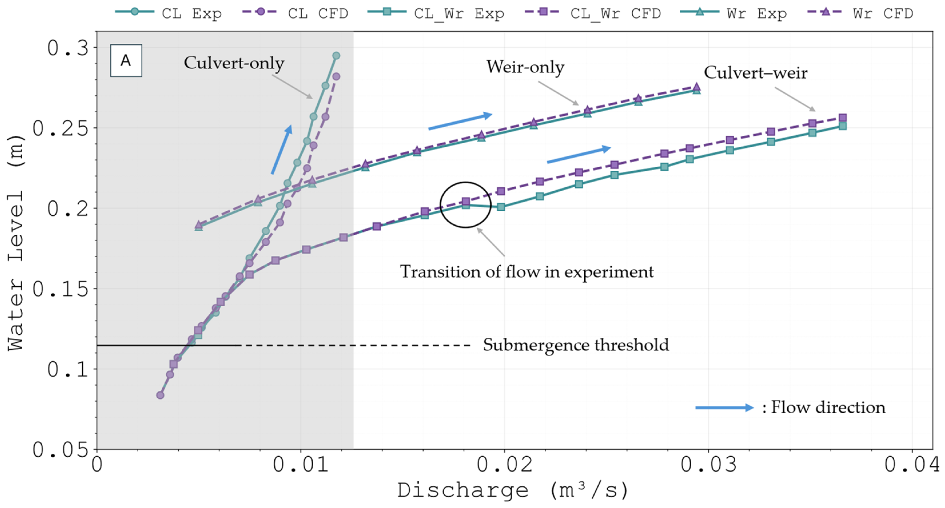
Rising limb: Figure 3 presents the steady state h Q curves for the rising limb experiments across the culvert-only (Cl), weir-only (Wr) and culvert–weir (Cl_Wr) configurations, providing a direct comparison between CFD model and experimental (Exp) data. The horizontal axis represents the discharge Q , which increases from low to high flows to construct the steady rising limb curves, while the vertical axis indicates the headwater elevation in meters recorded at the h 1 location. In these plots, the violet curves represent the CFD model values, and the green lines correspond to the experimental data.
A general trend could be observed across all three configurations: The headwater elevation increases as the discharge increases, and the numerical model effectively reproduces both the slope and the curvature of the experimental h Q curves during rising flows. Specifically, there is good agreement between the numerical and experimental data for the weir-only configuration. However, small discrepancies occur primarily at higher discharges for the culvert-only and combined culvert–weir configurations.
For the culvert-only test, the numerical model predicts a partially full culvert for all discharge levels. This is consistent with the experimental rising limb tests, where inlet behavior and the concentration of streamlines prevented the barrels from flowing full. In the culvert–weir case, the numerical model also predicts partially full flow at all discharges; however, the experiments indicate a transition to full culvert flow at higher discharges, as highlighted by the circled region in the figure. This divergence indicates that weir overflow and culvert outflow interaction changes the system dynamics relative to the culvert-only case and is associated with the observed regime transition behavior.
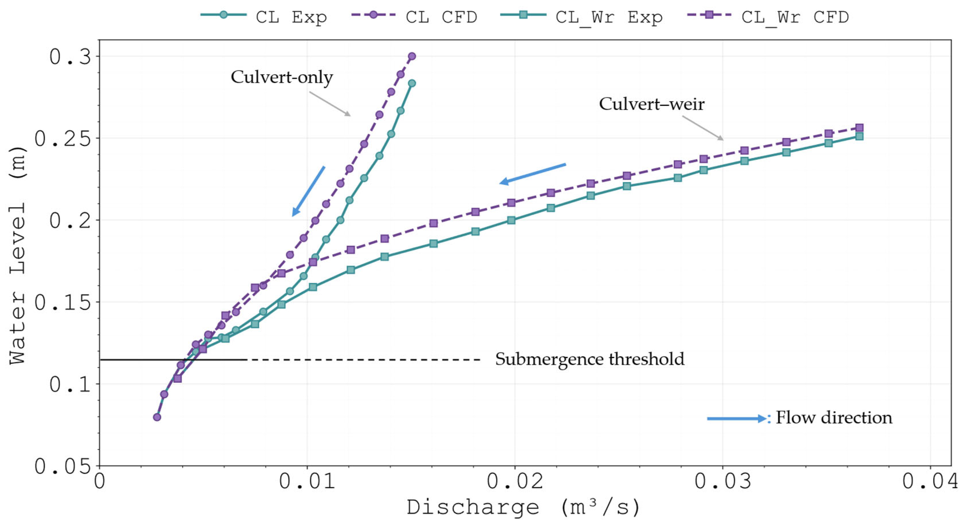
Receding limb: Figure 4 presents the h Q curves for the receding limbs of the culvert-only and culvert–weir configurations, providing a comparison between the numerical and experimental headwater elevations.
For both configurations, the headwater decreases monotonically while discharge reduces. The culvert–weir case shows that discrepancies between the numerical model and experiment increase as the discharge decreases. For the culvert-only configuration, the discrepancies are quite significant during the submergence phase, where the culvert flows full in the numerical simulation, which is consistent with the experimental observations. Furthermore, the transition from full to partially full flow occurs at approximately the same point in both the numerical and experimental models, specifically at a discharge of 4.63 L/s and a headwater level of 0.12 m. For the culvert–weir case, the numerical model predicts partially full flow across all discharge levels, whereas the experiments show a transition to partially full culvert flow only at the end of the submergence phase.

4.2. Mesh Verification and Local Inlet Diagnostics

4.2.1. Full-Geometry Mesh Verification

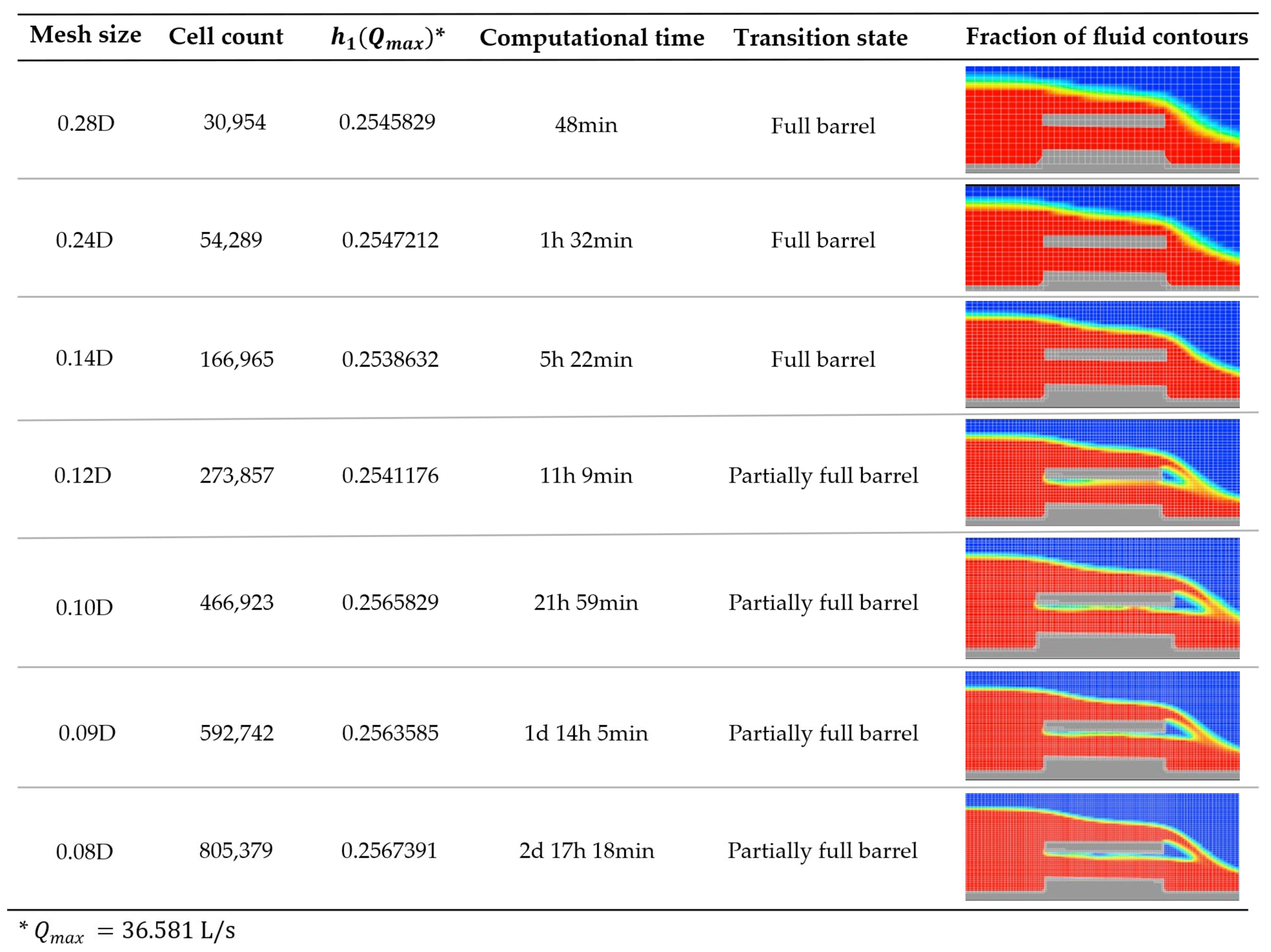
To assess mesh sensitivity in the complete culvert–weir geometry, seven resolutions ranging from 0.28D to 0.08D were compared using the same geometry, discharge sequence, boundary conditions and numerical settings. Figure 5 summarizes the mesh resolution, total cell count, computational time, predicted barrel state and representative VOF fields. The 0.28D, 0.24D and 0.14D meshes predicted a full-barrel state, whereas the 0.12D mesh and finer meshes predicted a partially full state over the tested discharge sequence.
The global headwater response also became progressively less sensitive with refinement as shown in Table 2; the mean absolute relative difference decreased from 0.47% for the 0.10D → 0.09D refinement to 0.17% for 0.09D → 0.08D, while the latter refinement increased the cell count by approximately 36% and the computational time by approximately 71%. For the global headwater response, this stabilization around 0.09D is consistent with the simplified mesh design analysis in Appendix B, where headwater became insensitive at approximately Δ l culv D / 10 , and is of the same order as the literature-based guidance cited in Section 3.2.2.
This consistency indicates that simplified case analyses and literature estimates can provide a useful first-order indication of the mesh scale required for more complex culvert–weir geometries. The full-geometry analysis further confirms the stability of the barrel state response between the two finest meshes, while detailed local inlet quantities may still require finer refinement. This consideration may be particularly relevant for circular culverts, where the curved barrel and inlet geometry is more demanding to represent on a Cartesian mesh; its applicability to box culverts, whose planar surfaces may be represented more directly, should be assessed separately.

4.2.2. Local Inlet Mesh Diagnostic Under Culvert-Only Flow Conditions

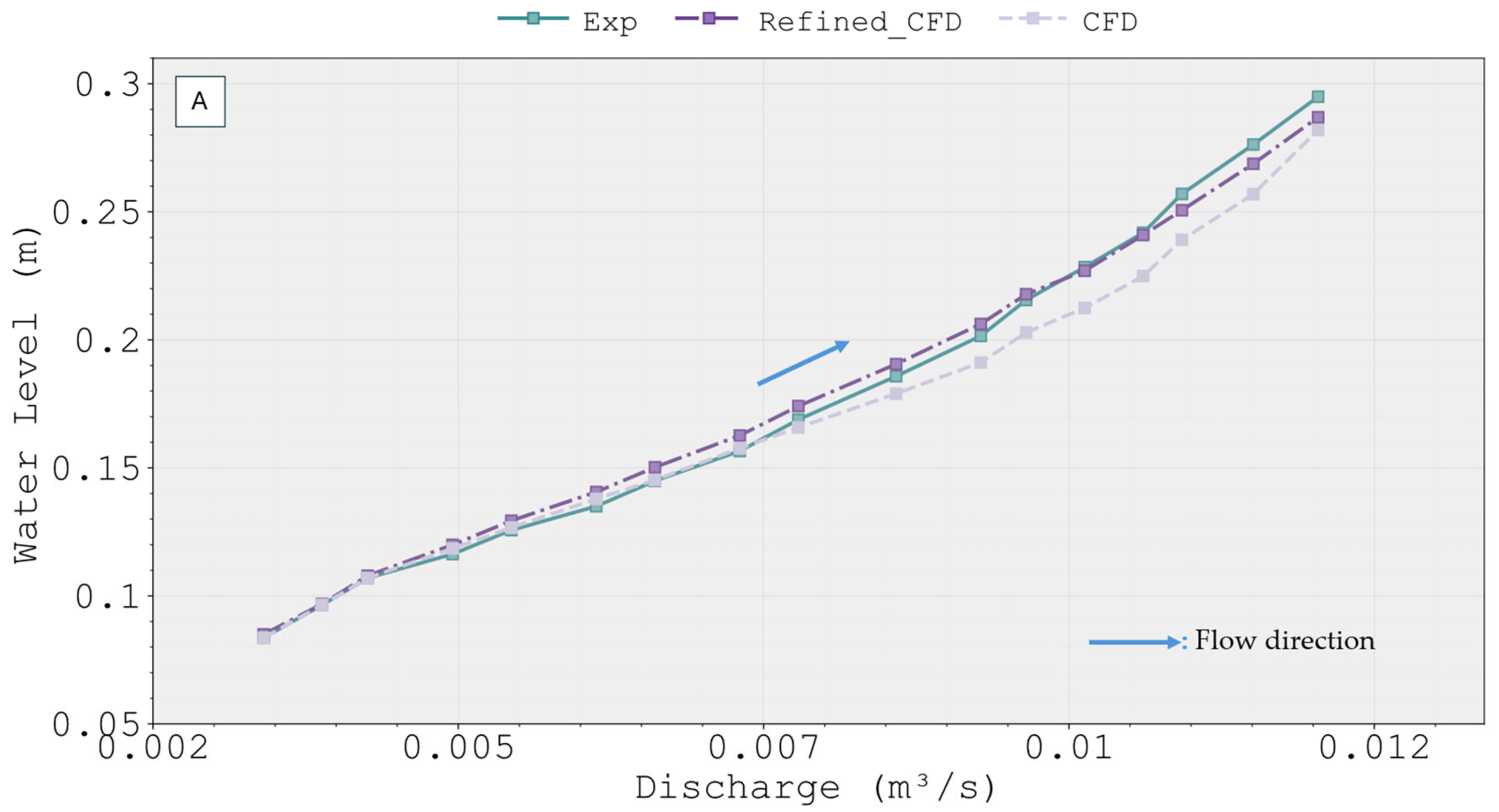
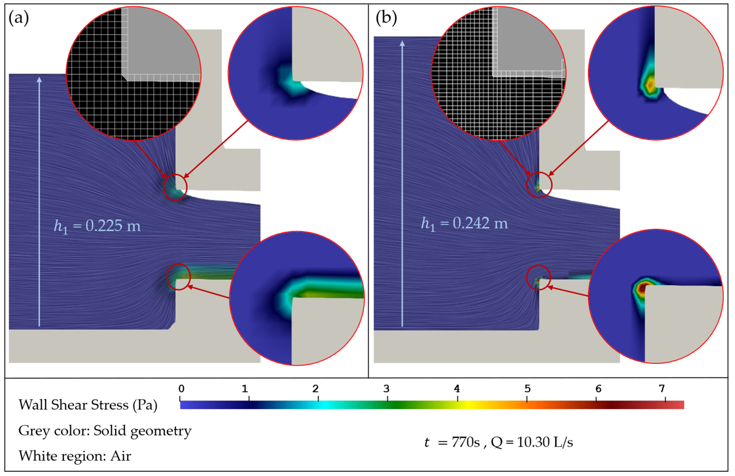
Rising limb: Investigation on the origin of the discrepancies observed for the culvert-only rising limb case showed that the creation of the mesh from the original geometry using the provided mesh generator induced a tapering of the inlet. This tapering allows smoother and more horizontal streamlines at the edge with respect to the reported sharp edges adopted in the lab experiment. This ultimately allows a higher degree of filling and thus a higher flow rate entering the culvert, as shown for the benchmark mesh in Figure 6a. A local inlet refinement diagnostic was therefore performed to examine whether a finer representation of the sharp inlet altered the predicted streamlines and associated headwater response. The mesh refinement consisted in reducing the cell size from Δ l = 0.09 D used in the benchmark case to Δ l = 0.02 D .
The region with Δ l = 0.02 D extended 1.5 D upstream and 1.5 D downstream of the inlet (inside the barrel). This region with Δ l = 0.02 D was not connected directly to the region with Δ l = 0.09 D . Rather, a transition region with Δ l = 0.046 D extending 0.75 D downstream and upstream was introduced.
Another considered aspect was the wall shear stress distribution at the culvert inlet edges for the benchmark and refined meshes, shown in Figure 6a,b, respectively. The quantitative differences between the two meshes are summarized in Table 3. The low wall shear stress in the benchmark mesh indicates weak resolution of inlet acceleration and separation, whereas the increased shear stress in the refined mesh indicates improved resolution of inlet losses, consistent with a sharper inlet and stronger local gradients.
Consistent with these local changes, Figure 7 shows that the refined CFD model lies closer to the experimental h Q points, with the largest improvement at higher discharges in the post-submergence region. This local inlet sensitivity was not identified by the global mesh sensitivity analysis and was instead revealed through the targeted inlet diagnostic. The remaining differences are small and occur mainly at the upper end of the discharge range. This behavior indicates that inlet region resolution affects streamlines and inlet losses and, in turn, the headwater response, with the baseline CFD model tending to underpredict water level after inlet submergence.
Receding limb: The h Q curve for the culvert-only receding limb case (Figure 4) shows that the numerical model predicts a higher headwater h 1 than the experimental measurements. It was found that additional inlet mesh refinement described in the previous subsection did not improve the performance, indicating that the mismatch is not caused by the poor inlet resolution alone.
The observed discrepancy during the receding limb may be influenced by uncertainties in experimental initialization and reporting, because the experimental sequence began under high-discharge conditions with full barrels and then progressively decreased. The experimental documentation did not fully document the procedure used to establish the initial full-flow state, including how the barrels were filled and how air was managed before drawdown. The resulting uncertainty in the initial hydraulic state therefore represents a possible contributor to the receding limb mismatch.
Findings from the integrated culvert–weir and unsteady analyses (Section 4.4 and Section 4.7) are consistent with this interpretation, suggesting that deviations in the rising limb terminal state may propagate into the receding limb trajectory. Consequently, receding limb hydraulics may be highly sensitive to antecedent aeration and flow conditions, and this interpretation is consistent with the observed differences in culvert flow behavior between the culvert-only and culvert–weir configurations. Differences in these initial states may therefore contribute to discrepancies in the observed drawdown response.

4.3. Additional Physics

The baseline configuration involved benchmark simulations that were initially conducted without considering the surface tension or air entrainment. To investigate the influence of these phenomena, three cases were performed for the culvert–weir steady state: the first included surface tension, the second incorporated air entrainment, and the third activated both models simultaneously. The results demonstrated that the inclusion of these two phenomena in the numerical setup led to no changes in the h Q relationship. This observed trend may confirm that water levels (at least at the spatial scales considered in this study) are not controlled or affected by these two phenomena.

4.4. Discrepancy Diagnosis for the Culvert–Weir Case

Particular attention was given to understanding the discrepancies observed in the culvert–weir configuration, as this case is especially relevant to real-world applications. The culvert–weir system represents a combined condition in which conveyed flow through the culvert and excess flow due to overtopping occur simultaneously, a scenario commonly encountered during high-stage and extreme events in practice.
Rising limb: For the rising limb, the discrepancy is associated with regime behavior: the numerical model keeps the culvert partially full, whereas the experiments show a partial to full transition at higher discharges (circled region in Figure 3). After inlet submergence, the barrels are 90% full in the numerical model, which may explain the higher value of h 1 obtained with the numerical model relative to the experimental h 1 .
The laboratory study states that each prescribed discharge level was maintained for a sufficient duration to achieve quasi-steady water levels before recording. However, the transition or ramp time between successive discharge plateaus is not documented, which introduces uncertainty regarding the imposed d Q / d t . This lack of data potentially contributes to the observed discrepancies between the numerical and experimental results.
We note that, in the numerical simulations, we used experimentally defined constant-discharge levels over plateau periods, with each plateau connected to the next by a ramp of duration Δ t r . A sensitivity of the results on the discharge ramp time Δ t r was indeed observed.
More specifically, Δ t r influences the so-called “ventilation state” of the outlet, namely, the presence or absence of a void gap at the culvert outlet. To better investigate this aspect, a targeted ramp history investigation was performed by varying the discharge ramp time that influences the rate of change of flow as d Q / d t ( Q i Q i 1 ) / Δ t r . This approach was motivated by the unreported ramp timing between plateaus, which for this reason was to be treated as an uncertainty potentially affecting the results.
In this framework, the primary objectives were: (i) to understand the numerical behavior behind the discrepancies, and the corresponding potential issues in practical applications; (ii) to assess whether plausible variations in Δ t r could alter the occurrence and timing of the regime transition; and (iii) to examine the relationship between Δ t r   and the outlet ventilation state, which governs the attachment or detachment behavior between the weir overflow and the culvert outflow.
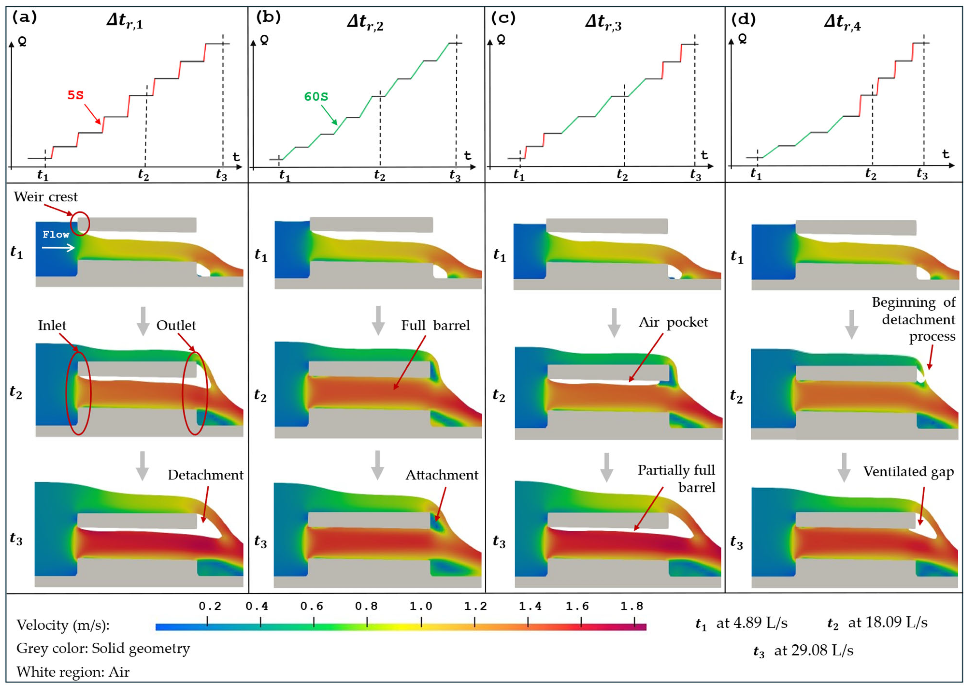
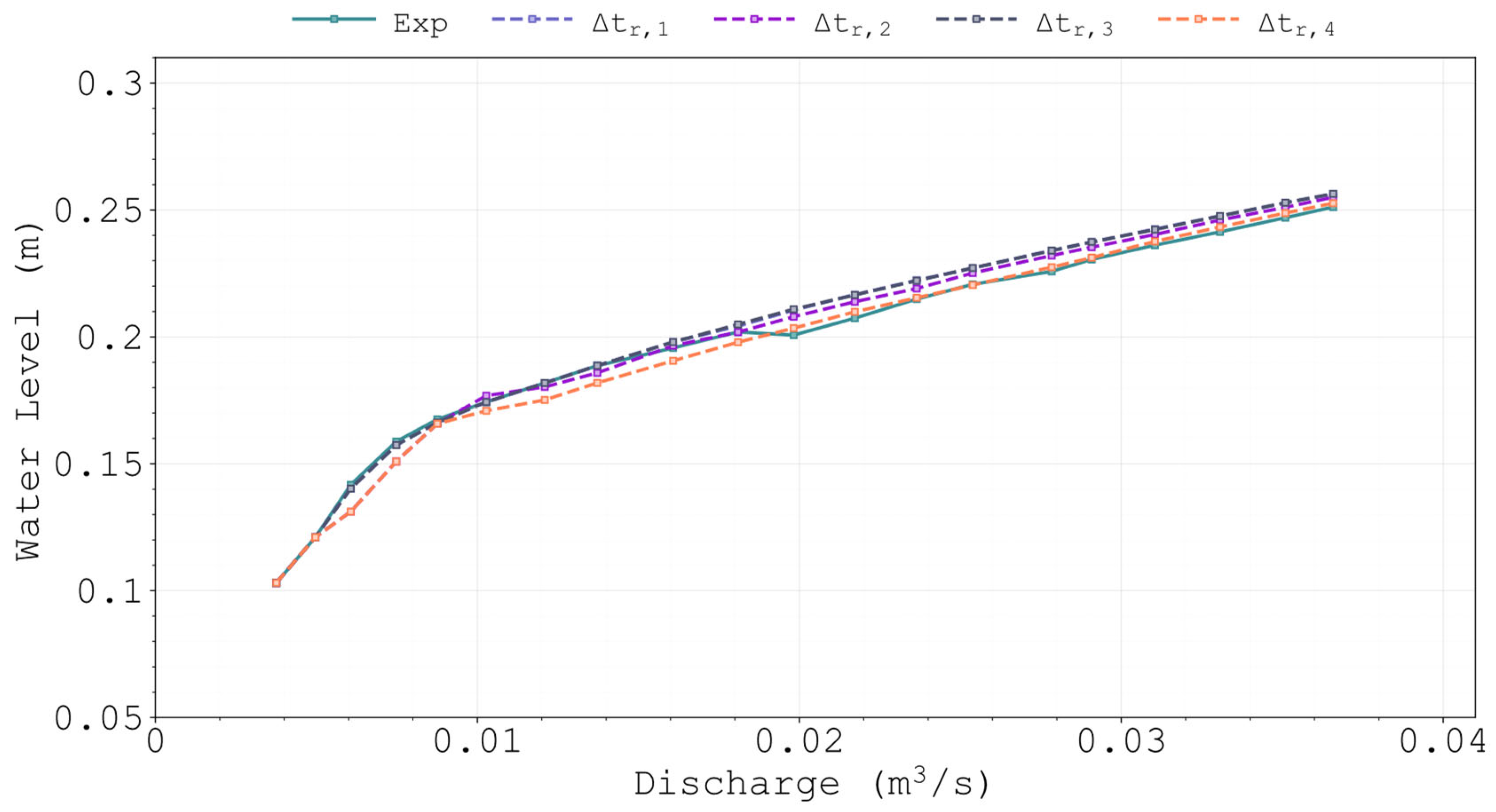
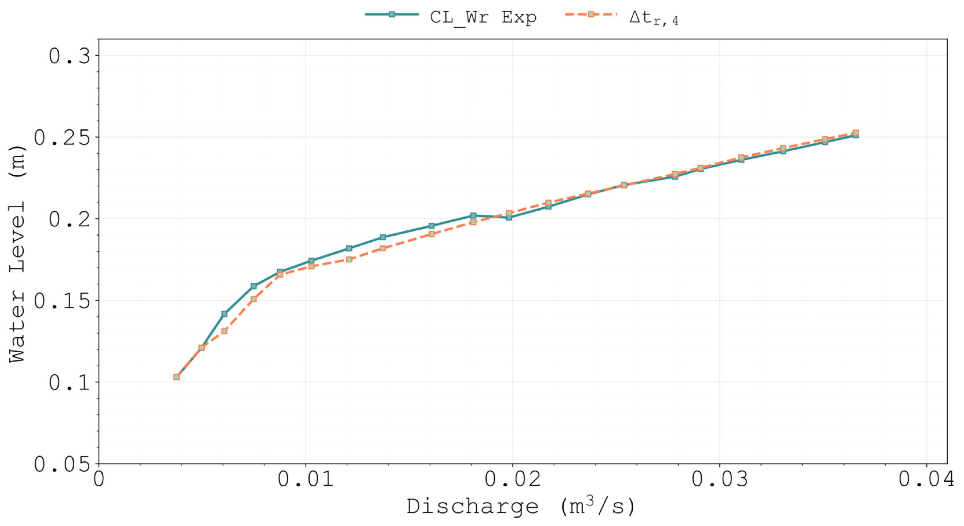
In the ramp time sensitivity test, we considered the same sequence of discharge plateaus (with each plateau held for a constant stabilization time of Δ t p = 60 s to allow for the evaluation of water levels and regime indicators at the end of each period). The test consisted in variations of the ramp time Δ t r between successive plateaus, thereby altering d Q / d t without modifying the discharge magnitudes. Four distinct ramping cases were tested. The first (benchmark case) was a fast ramp where Δ t r , 1 = 5 s was applied for all steps, while the second was a slow ramp with Δ t r , 2 = 60 s for all steps. The third case, identified as the first hybrid ramp Δ t r , 3 , followed a sequence of 5 s for discharges below 10.27 L/s, 60 s for discharges from 10.27 L/s to 21.72 L/s and 5 s thereafter, emphasizing slower ramp times for the critical value of discharges where transition from partially full to pressurized occurs in experiments. Finally, the second hybrid ramp Δ t r , 4   utilized 60 s for discharges below 16.08 L/s and 5 s for discharges exceeding this value, emphasizing slower ramp times for the lowest discharges.
Figure 8a–d presents the velocity magnitude contours on a 2D centerline slice of the first culvert barrel for Δ t r , 1 , Δ t r , 2 , Δ t r , 3 and Δ t r , 4 , respectively, illustrating the influence of the four inflow ramping strategies on outlet attachment, ventilation and the resulting culvert flow regime. The barrel and outlet states discussed below were classified using the VOF-based criterion defined in Section 3.2.5.
The trends observed in Figure 8a (the fast ramp case) show that at t 1 the flow submergences the inlet. By t 2 , the rapid increase in discharge produces the overtopping of the inlet, the activation on the weir flow and an overflow jet that projects away from the culvert outlet, ensuring the weir overflow remains detached from the culvert outflow. At   t 3 , a distinct air region persists at the culvert outlet, which indicates sustained ventilation while the barrel remains partially full. The fast ramp maintains a stable detached configuration with a ventilated state and a partially full barrel across the rising limb, resulting in no regime transition.
In contrast, Figure 8b details the behavior under a slow ramp case. Following inlet submergence at t 1 , the gradual increase in discharge at t 2 (low value of d Q / d t ) does not allow the formation of a jet. Rather, the flow creeps and keeps the overflow close to the outlet; consequently, attachment develops and the barrel reaches a full-flow condition. By t 3 , this attachment persists without a ventilated gap, and the barrel remains full. The slow ramp thus promotes attachment and sustains a sealed full-barrel state at later stages, causing the flow regime transition to occur at flow rate lower than those observed in experiments.
Figure 8c then shows the behavior under the first hybrid ramp time case. The initial behavior at t 1 aligns with cases (a) and (b). However, at t 2 , the slow ramping segment facilitates attachment between the weir overflow and culvert discharge, inducing air-pocket formation along the upper barrel. A subsequent transition to accelerated ramping at t 3 triggers jet detachment and restores outlet ventilation, resulting in a partially full regime. This ramping sequence does not induce a complete flow transition; the persistent air pocket maintains a partially full state even at peak discharge.
Finally, Figure 8d details the behavior under the second hybrid ramp time case. The initial behavior at t 1 aligns with cases (a–c). At t 2 , accelerated ramping initiates jet detachment and the onset of outlet ventilation. By t 3 , a distinct ventilated gap is established and the outlet is fully detached, while the barrel maintains a full-flow regime. This ramping sequence evolves from an initially attached state toward progressive detachment. This culminates in a stable ventilated gap and sustained full-barrel flow at elevated discharges, demonstrating that full barrel can coexist with later outlet ventilation. The imposed ramp histories and their corresponding regime and outlet states are summarized in Table 4.
The observed sequence demonstrates that the ventilation state is strongly dependent on the discharge rate of change ( d Q / d t ) rather than absolute magnitude. Accelerated ramping favors a detached, ventilated outlet and partially full flow; conversely, gradual ramping promotes early sealing and attachment, facilitating full-barrel conditions. While hybrid ramping fails to provide deterministic control over transition timing, these cases confirm the pronounced path-dependency of the ventilation state relative to the temporal variation in discharge.
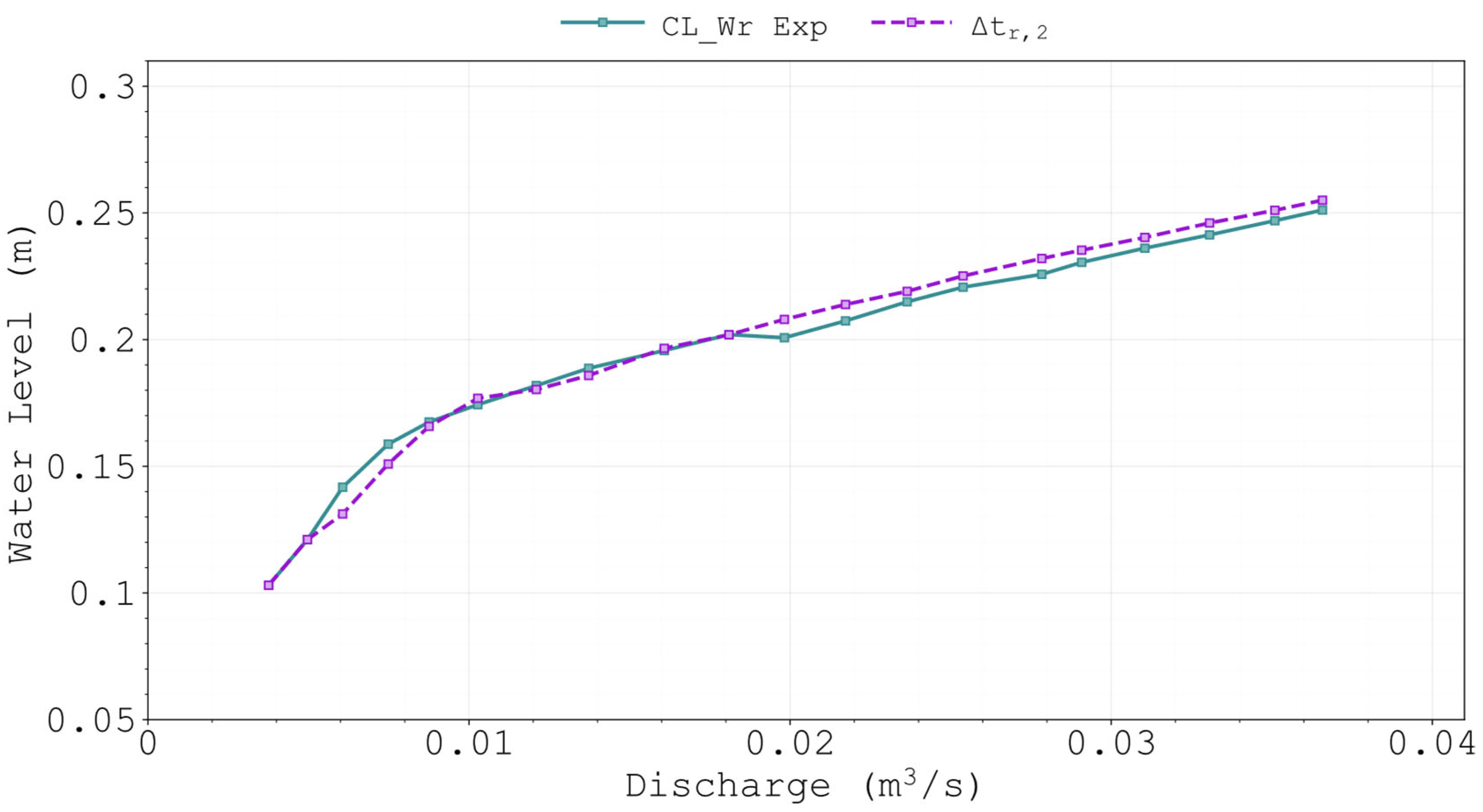
Figure 9 compares the h Q relationships with the experimental data during the rising limb for different ramp time strategies. The numerical cases reproduce the experimental trend well, with minor discrepancies at medium to high discharges (refer to Appendix C for a more detailed chart). At high discharges, Δ t r , 3   gives the highest water levels and the largest positive bias. The fast ramp Δ t r , 1   also overpredicts water levels at high discharges, but less than Δ t r , 3 . The slow ramp Δ t r , 2 slightly underpredicts water levels at low discharges and then approaches the experimental curve as discharge increases. The Δ t r , 4 case remains closest to the experiment at high discharges, with minor discrepancies at low discharges.
These results show that the rising h Q relationship is sensitive to the imposed ramping history, even when the discharge plateaus are identical. Among the tested cases, Δ t r , 4   gives the best overall agreement. No regime transition was observed for Δ t r , 1   and Δ t r , 3 . In contrast, both Δ t r , 2   and Δ t r , 4 produced a transition, but at lower flow rates than the experimental transition discharge. These comparisons were used diagnostically, and the Δ t r , 4 case was not substituted for the benchmark validation case.
Receding limb: The rising limb discrepancy analysis did not resolve the regime transition mismatch, as fast ramps remained partially full and ventilated, whereas slow ramps transitioned too early and remained attached. Consequently, the experimental transition could not be reproduced robustly. Because the culvert–weir experiment is continuous, the recession begins from the hydraulic state established at the end of the rising limb. A mismatch in the predicted rising limb terminal state may therefore influence the subsequent receding limb comparison. Accordingly, the receding limb comparison is interpreted in light of the rising limb end state.

4.5. Sensitivity Analysis on the Turbulence Model Adopted

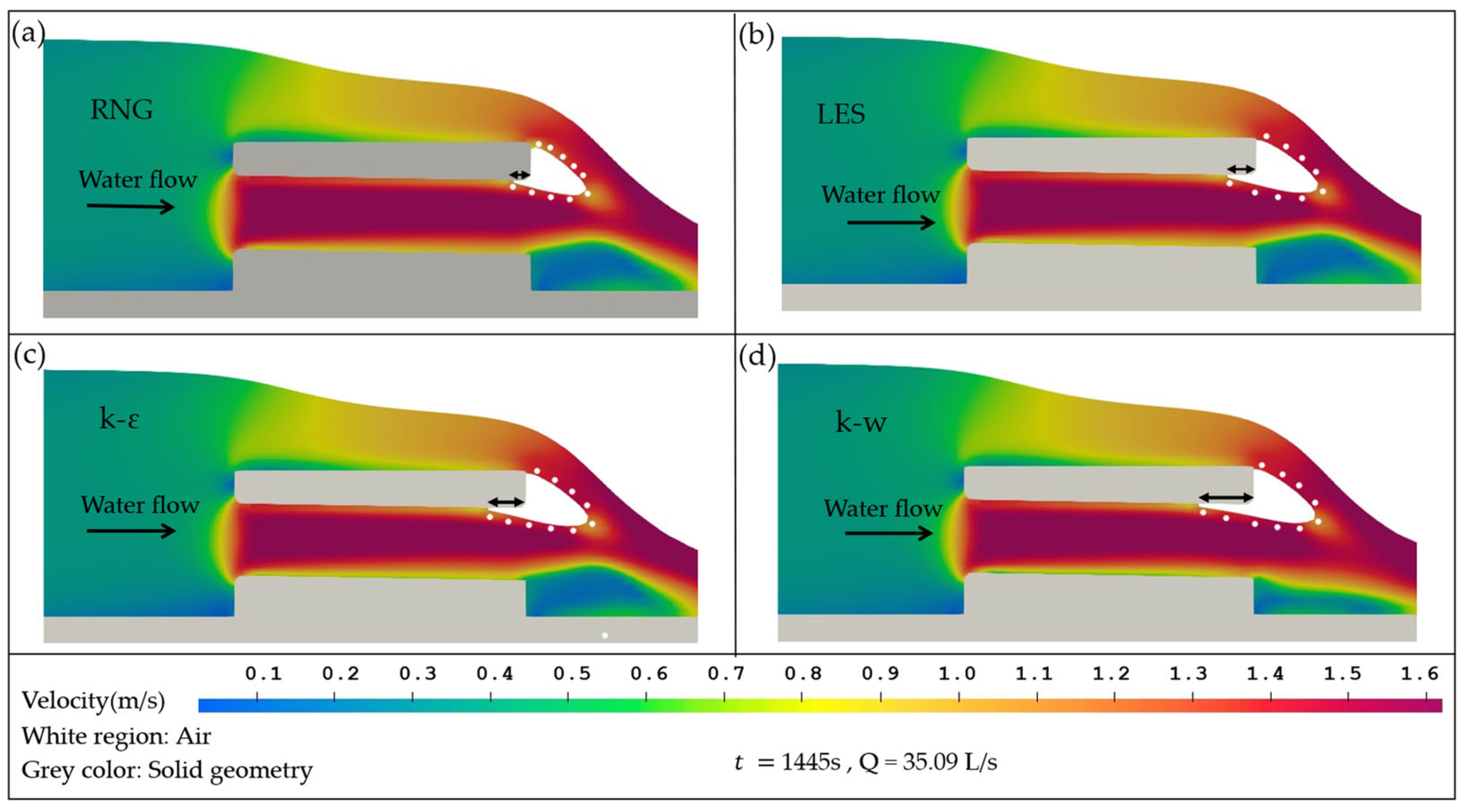
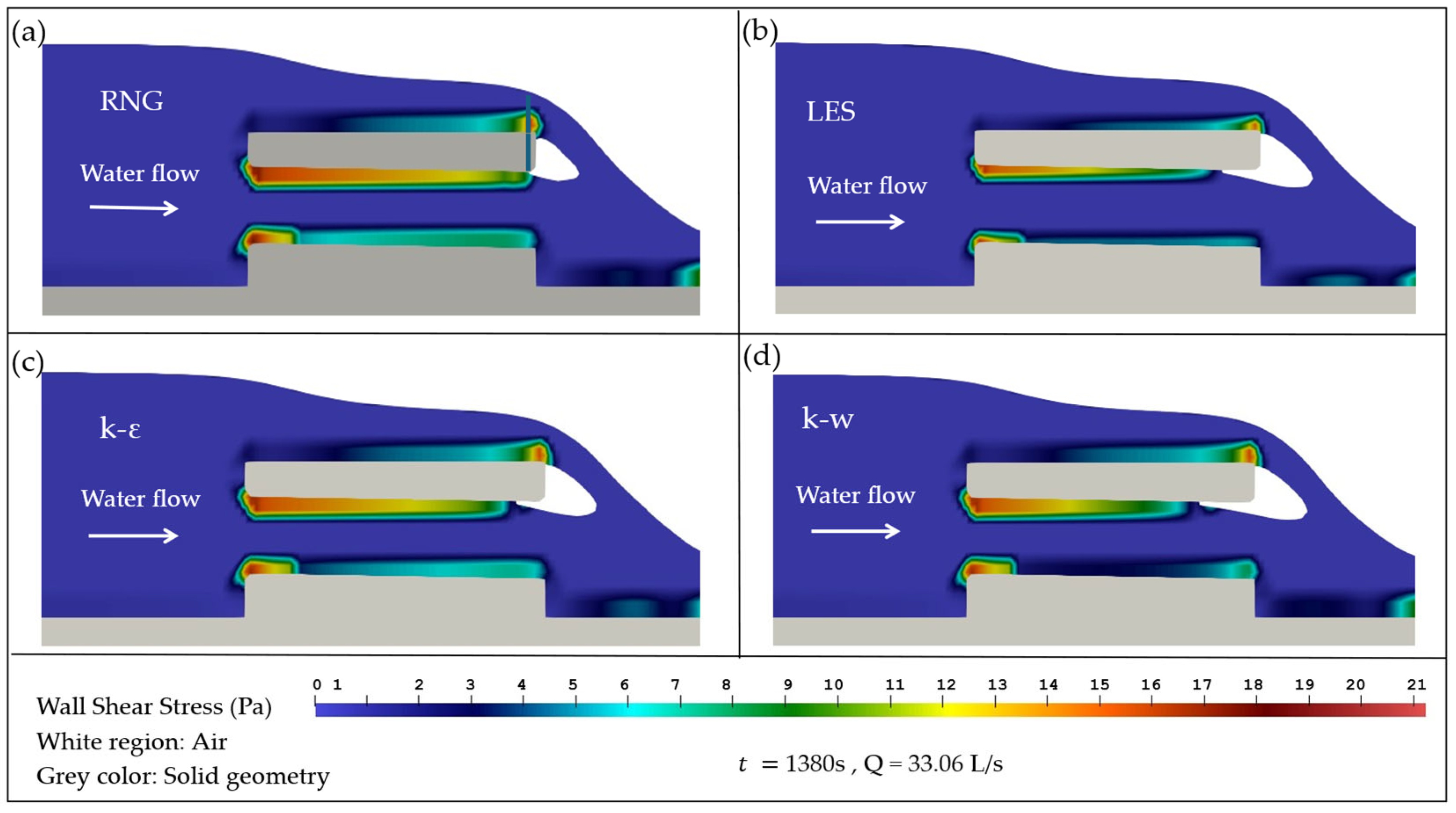
Sensitivity analysis assessed turbulence model influence on the culvert–weir rising limb case with ramping time Δ t r , 4 . Standard k ε , k ω and large eddy simulation (LES) closures were evaluated against the RNG k ε (benchmark model).
Figure 10 shows that turbulence closure affects the degree of barrel filling and the associated air-pocket morphology. The k–ω model produces the most pronounced incomplete filling and air-pocket formation near the outlet, whereas RNG k–ε produces the greatest barrel filling.
Figure 11a–d compares wall shear stress (WSS) distributions for RNG, LES, standard k–ε and k–ω, respectively. The RNG and standard k ε schemes produce relatively uniform WSS profiles along the culvert and weir boundaries. Conversely, the k ω model yields sharp, localized peaks near the entrance, whereas LES results exhibit low-magnitude, spatially variable shear fields. The main differences among the turbulence closures are summarized in Table 5.
In summary, turbulence model selection affects the predicted barrel filling, air-pocket morphology, and wall shear stress; however, the global water stage remains insensitive to the closure scheme in this specific geometry.

4.6. Statistical Comparison (RMSE, MAE, R2, MARE)

The statistical validation of the benchmark CFD configuration against the experimental data is summarized in Table 6. The weir-only rising case shows strong agreement and the lowest error levels among the rising limb cases. The culvert-only case shows good reproduction of the rising limb. The culvert–weir rising case with Δ t r , 1   shows good agreement, but with a slightly lower performance than the culvert-only and weir-only rising cases.
Overall performance is strongest for rising limb simulations, indicating reliable capture of increasing-flow conditions. The culvert–weir case is more sensitive than culvert-only and weir-only cases, consistent with added overtopping–culvert interaction. The lower culvert–weir receding agreement is consistent with recession dependence on the rising limb end state and outlet ventilation or attachment mode.

4.7. Unsteady State

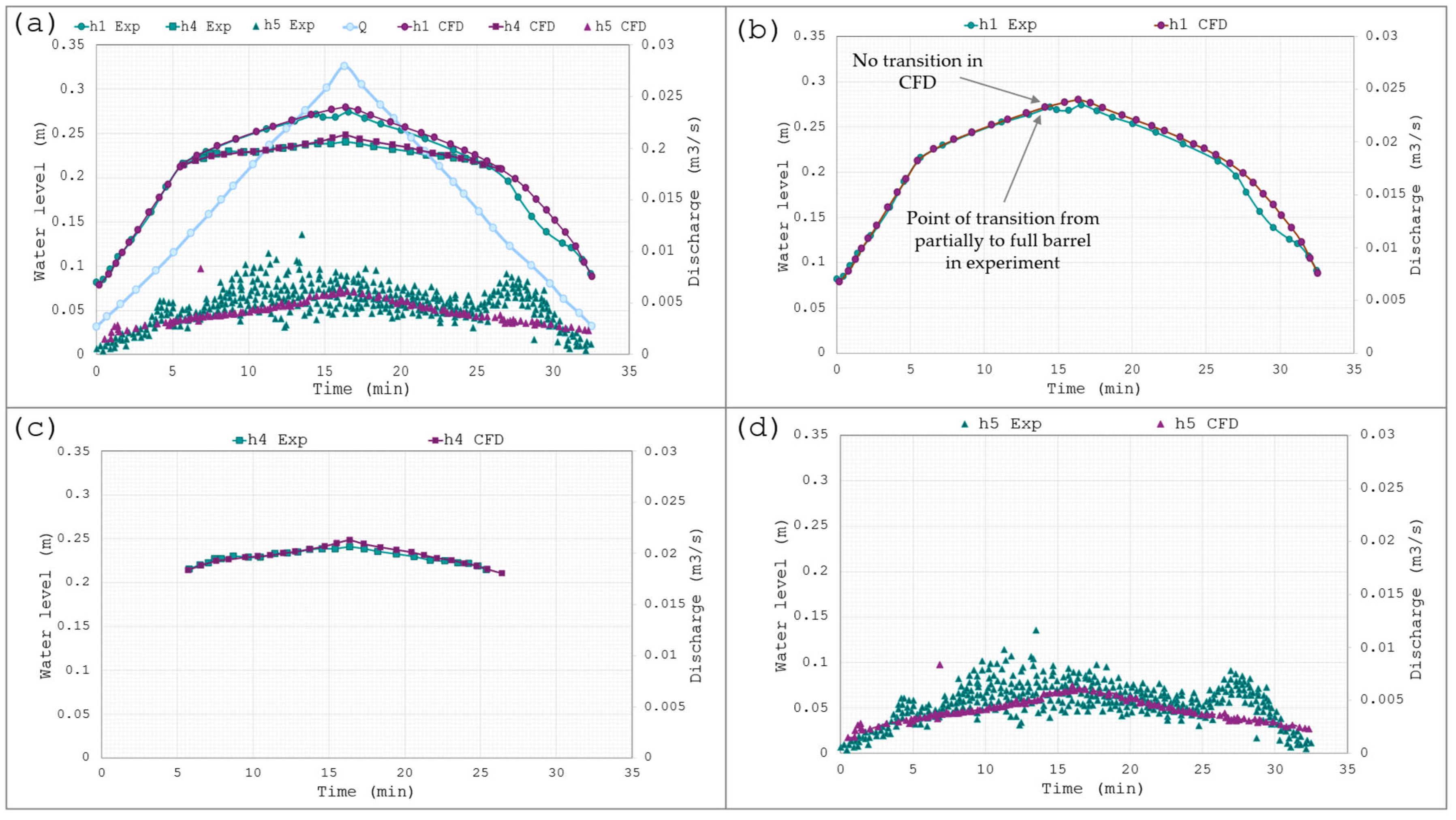
For the unsteady state, the benchmark runs use the same physical flume and culvert–weir setup as in the steady state case, replicated numerically using incompressible RANS with VOF free surface tracking and FAVOR geometry representation and performed with the RNG k–ε turbulence mode. Measurements are taken at h 1 upstream headwater, h 4 above the weir crest and h 5 downstream.
The results of the unsteady free-flow culvert–weir test are presented in Figure 12a–d, showing the full measurement set, the upstream response at h 1 , the weir-crest response at h 4 and the downstream response at h 5 , respectively.
Analysis of the trends in Figure 12b shows that at h 1 , both the experimental and numerical responses follow a consistent rise-to-peak-to-recession pattern. The quantitative comparison in Table 7 gives an RMSE of 9.35 mm, an MAE of 6.34 mm and R 2 = 0.9776, with a peak stage error of 5.6 mm and a peak time error of 12.25 s. The numerical response exhibits slightly higher water levels during the late recession phase. In the experiment, a transition occurs close to the peak, whereas the numerical model remains partially full throughout the entire hydrograph. At h 4 , Figure 12c shows similar experimental and numerical water level evolution above the weir. The corresponding RMSE and MAE are 3.02 and 2.20 mm, respectively, with R 2 = 0.8135; the peak stage error is 7.7 mm, and peak time error is 0.26 s. At h 5 , Figure 12d shows that the experimental record is scattered but follows an overall rise-and-fall trend, while the numerical model reproduces the mean trend but not the short-term fluctuations, with larger differences during recession. Because the experimental downstream record is strongly scattered, pointwise and peak-based metrics were not considered sufficiently robust at this location; the h 5 comparison is therefore retained as a qualitative assessment.
The largest differences, occurring at h 5 , are consistent with the higher variability and noise present in downstream measurements and the greater sensitivity of downstream levels during drawdown. Overall, the quantitative metrics support good reproduction of the unsteady water stage response at h 1 and h 4 , while the downstream h 5 comparison and the unresolved partial-to-full transition require greater caution.

4.8. Dimensionless Characterization

The dimensionless ranges represented by the steady and unsteady benchmark cases are summarized in Table 8. These values provide a scale-independent description of the hydraulic conditions covered by the present simulations. Because h*, Q *,   F r and R e were not varied independently, the reported ranges are not interpreted as general regime thresholds; instead, they provide a common dimensionless basis for the subsequent discussion of model performance, regime behavior and mesh sensitivity.

5. Discussion

The strong agreement, maintained across the tested weir-only range ( Q = 0.994 5.860 ) , indicates that the numerical model effectively captures the dominant crest control and overtopping hydraulics. This suggests that any remaining errors are more likely associated with the culvert regime representation rather than the weir formulation itself. The observation that discrepancies grow primarily towards the higher h and higher Q portion of the tested range for the culvert-containing configurations supports the conclusion that the modeling challenge is concentrated within the transition range, involving submergence and mixed behavior. In this range, the flow is close to filling the culvert crown, meaning small changes in predicted energy losses or the ventilation state can determine whether the computed water surface reaches the crown and causes the barrel to become full.
For the culvert-only rising tests, both the numerical simulations and experiments indicate partially full flow across the tested discharges. This implies that inlet conditions govern the response: the inlet flow contraction and concentration of streamlines limit barrel filling and prevent full-barrel flow. The numerical model is therefore consistent with the observed inlet-controlled behavior. In the culvert–weir rising limb case, the persistent partially full state in the numerical model, contrasting with the experimental transition to full flow, indicates that the interaction between overtopping flow and culvert outflow modifies the outlet condition in a way that is critical for pressurization, implicating the outlet sealing or ventilation pathway in the transition behavior.
Ramp time sensitivity tests demonstrate two stable outlet modes, identified as detached/ventilated state associated with lower t r and higher Γ and attached/sealed state associated with higher t r and lower Γ . This implies that the transition is controlled by the outlet topology, specifically whether the air pocket is maintained or suppressed, rather than being solely determined by discharge magnitude. The hybrid ramp cases reveal that once a ventilated state is established, it can persist through subsequent changes in ramping. This helps explain why adjusting the ramp rate only within the critical discharge range may still fail to initiate the transition observed in the experiments. Such behavior aligns with mixed-flow research, showing that air-pocket evolution and sealing–unsealing processes can produce different pressurization pathways for the same discharge range under varying inflow histories [50,51].
The analysis of inlet mesh refinement, which increased wall shear and improved agreement for the culvert-only rising limb, supports the conclusion that inlet losses are under-resolved on coarse grids. It further confirms that within the higher h and higher Q portion of the tested culvert-only range after submergence, the headwater elevation is sensitive to entrance sharpness and local gradients. However, the fact that inlet refinement did not improve the culvert-only receding limb agreement indicates that entrance resolution alone does not explain the discrepancy; uncertainty in the initial hydraulic state and the preceding air and barrel filling history may also contribute.
Furthermore, the limited impact of activating the surface tension and air entrainment options on the water stage suggests that, for the present setup and conditions, the bulk stage–discharge response is not sensitive to these model additions. By contrast, differences in barrel filling and air-pocket extent across turbulence models indicate that regime prediction depends on how flow detachment, recirculation and near-wall stresses are represented, particularly within the outlet interaction zone. Statistically, the larger discrepancies found in the culvert–weir receding case compared with the experiment occur in a continuous experimental sequence in which the recession begins from the end state of the rising limb. The transition state mismatch occurring during the rising limb may therefore contribute to the receding limb discrepancy.

6. Conclusions

This study evaluated whether a CFD model (FLOW-3D) can be used with confidence for culvert hydraulics relevant to urban drainage and extreme event scenarios. The focus was on stage prediction, overtopping behavior and flow regime transitions, considering culvert-only, weir-only and combined culvert–weir flows. Numerical results were compared with published laboratory data for a single benchmark geometry across steady sequences and an unsteady hydrograph. The main conclusions drawn by this study can be summarized as follows:
  • The CFD model reproduced the main water stage response across the tested configurations. For the reported steady benchmark comparisons, MARE ranged from 0.90% to 5.42%. Under the unsteady hydrograph, h 1 yielded RMSE = 9.35 mm, MAE = 6.34 mm and R 2 = 0.9776, with peak stage and peak time errors of 5.6 mm and 12.25 s, respectively; at   h 4 , the corresponding values were 3.02 mm, 2.20 mm, R 2 = 0.8135, 7.7 mm and 0.26 s. These results indicate that the principal water stage response was reproduced with generally small absolute errors.
  • Inlet mesh refinement was found to be a key parameter that strongly influences the representation of inlet flow contraction and separation, the associated entrance losses and the post-submergence headwater response in the culvert-only rising case. This indicates that sufficiently fine local resolution is particularly important when detailed inlet hydraulics influence the predicted headwater.
  • Discrepancies in the receding limbs could usually not be reduced, suggesting that recession behavior may be influenced by history or initialization effects. From a practical flood risk assessment perspective, this may represent a comparatively limited concern when the assessment is focused on peak conditions as it mainly affects the post-peak recession after the maximum flow has passed.
  • Despite the generally good reproduction of water stage, for the culvert–weir configuration, a key issue remains the partial-to-full regime transition. The CFD model did not consistently reproduce the experimentally observed transition and remained partially full when the experiment transitioned to full flow at higher discharge. This aspect was investigated by a ramp time sensitivity analysis that showed two possible outlet modes: detached and ventilated associated with partially full flow, versus attached and sealed associated with full-barrel flow. The ramp history analysis further showed that inflow history can alter outlet attachment and detachment, ventilation state and barrel filling even over the same discharge sequence, making regime transition prediction more sensitive than water stage prediction to the preceding hydraulic state.
  • Although the validation is based on one published laboratory dataset and a single benchmark geometry, the selected culvert–weir system covers a broad range of hydraulically relevant conditions, including partially full culvert flow, inlet submergence, weir overtopping, changes in outlet attachment and ventilation and the transition towards full-barrel flow. The scope nevertheless remains limited to this geometry and to free-flow/free-outfall conditions, without an independent second validation dataset. In addition, the experimental discharge ramp timing and initial hydraulic state were not fully documented, and the experimentally observed partial-to-full transition was not reproduced consistently. Further work should therefore test the identified numerical and hydraulic sensitivities using independent datasets spanning additional geometries, tailwater conditions, Froude number ranges and hydrograph shapes.

Supplementary Materials

The following supporting information can be downloaded at: https://www.mdpi.com/article/10.3390/w18172081/s1, The supplementary package contains the processed datasets used for the main headwater–discharge comparisons, ramp-time sensitivity analysis, mesh-sensitivity analysis, and statistical metrics, and a README file describing the contents.

Author Contributions

Conceptualization, Y.B., R.V. and P.C.; methodology, Y.B., R.V. and P.C.; software, Y.B.; validation, Y.B.; formal analysis, Y.B.; investigation, Y.B.; resources, Y.B., R.V. and P.C.; data curation, Y.B.; writing—original draft preparation, Y.B.; writing—review and editing, R.V. and P.C.; visualization, Y.B.; supervision, R.V. and P.C.; project administration, R.V. and P.C.; funding acquisition, P.C. All authors have read and agreed to the published version of the manuscript.

Funding

This study was carried out within the RETURN Extended Partnership and received funding from the European Union Next-Generation EU (National Recovery and Resilience Plan—NRRP, Mission 4, Component 2, Investment 1.3-D.D. 1243 2/8/2022, PE0000005, Spoke TS 2).

Data Availability Statement

The processed datasets supporting the main headwater–discharge comparisons, ramp time sensitivity analysis, mesh sensitivity analysis and statistical metrics are provided as Supplementary Material. The laboratory benchmark data were obtained from Meselhe and Hebert [6]. Additional simulation-related files are not readily available because of file size limitations, software-specific formats and data management constraints, but may be made available by the corresponding author upon reasonable request, where feasible.

Acknowledgments

The use of artificial intelligence in this paper was limited to grammatical refinement and typographical error detection. All scientific reasoning, methodological design and conclusions were developed by the authors.

Conflicts of Interest

The authors declare no conflicts of interest.

Abbreviations

The following abbreviations and symbols are used in this manuscript:
CFDComputational fluid dynamics
1D, 2D, 3DOne-, two-, three-dimensional
VOFVolume of fluid
FAVORFractional area/Volume obstacle representation
RANSReynolds-averaged Navier–Stokes
RNGRenormalization group
LESLarge eddy simulation
WSSWall shear stress
h Headwater level
Q Discharge
D Diameter
L Length
h cfd CFD headwater level
h exp Experimental headwater level

Appendix A

Appendix A.1. Experimental Apparatus

The experimental flume was 3.20 m long, 0.438 m wide and 0.305 m deep. The upstream face of the culvert–weir structure was located 1.44 m from the upstream end of the flume. The weir crest was 0.154 m above the flume bed. The two circular culvert barrels had a diameter of 0.0762 m and a length of 0.381 m. Their inlet and outlet invert elevations were 0.0432 m and 0.0381 m, respectively, corresponding to a culvert slope of 1.333/100. The barrels were arranged symmetrically, with their centers located 0.0762 m from the structure centerline.
The flume had a glass bed and walls supported by a stainless steel frame, with the head and tail tanks also made of stainless steel. The system was served by a pumping arrangement consisting of a variable-discharge pump and an orifice meter used to monitor the flow rate range.

Appendix A.2. Experimental Boundary Conditions

The upstream flow was supplied from a head tank by a variable-discharge centrifugal pump, using diffuser screens and a perforated wall at the entrance. For the steady tests, the discharge was set to successive constant values, whereas for the unsteady tests, the pump speed was varied to impose the prescribed hydrograph. Downstream, the tailwater was controlled in the laboratory by a sluice gate.
The present study considers only the published free-flow experiments for which the required data are fully reported. Under these conditions, downstream tailwater does not impose control on the culvert–weir response. The corresponding numerical boundary conditions adopted in the present study are described in Section 3.2.3.

Appendix A.3. Experimental Instrumentation and Measurement Procedure

Water level was measured using ultrasonic transducers at six longitudinal monitoring locations: h 1 = 0.66 m, h 2 = 1.00 m, h 3 = 1.35 m, h 4 = 1.70 m, h 5 = 1.96 m and h 6 = 2.81 m, measured from the upstream end of the flume. During the steady tests, water levels at all six locations were recorded for each discharge once steady flow was established. In the unsteady tests, water levels and discharge were recorded continuously throughout each experimental run. The present unsteady CFD comparison uses the experimental records at h 1 , h 4 and h 5 , corresponding to the upstream, weir region, and downstream monitoring locations, respectively.
Flow rate was measured using an orifice meter and differential pressure transducers installed in the discharge line. For the steady tests, discharge was measured through the orifice system together with the water level measurements for each steady increment. For the unsteady tests, discharge was continuously recorded alongside the water levels throughout the hydrograph.

Appendix B

Appendix B.1. Mesh Design Analysis

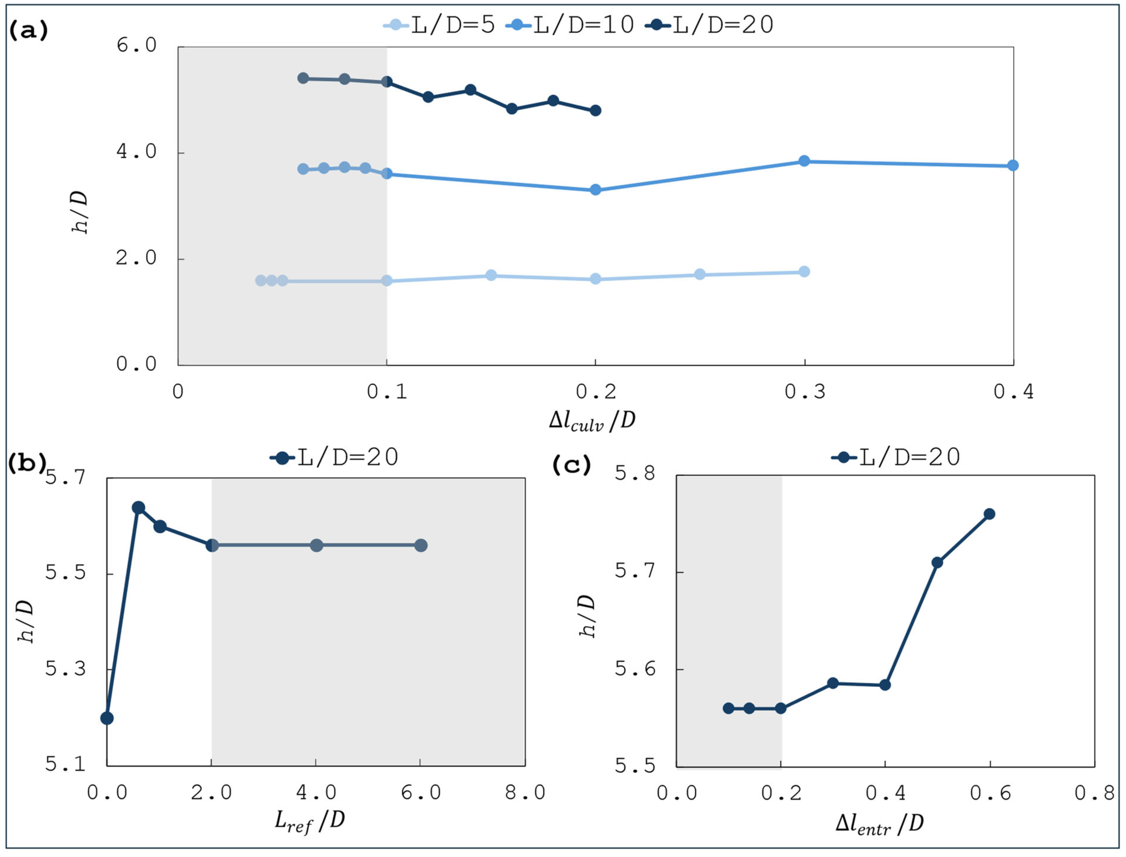
Prior to the benchmark simulations, a tripartite mesh design analysis was conducted using simplified culvert configurations to isolate the effects of individual refinement choices and provide practical guidance for constructing an efficient baseline mesh for the global headwater response. This study systematically evaluated three key parameters, as illustrated in Figure A1: (i) the discretization of the culvert region, (ii) the extension (length) of the refined upstream approach region ( L ref ) required to mitigate the effects of a coarser mesh in the entrance region and (iii) the discretization of the entrance region.
Figure A1. The 2D computational geometry (grey) and block-structured mesh (blue lines). Grey regions represent solid geometry.
Water 18 02081 g0a1

Appendix B.2. Method

Simulations utilized a single circular culvert with slope 1 / 1000 and lengths L = 5 D , 10 D   a n d   20 D . Discharge boundary conditions were set to achieve inside the culvert the average velocities U = 4.456   m / s , U = 6.366   m / s and U = 10.186   m / s . Each simulation ran for 50 s to ensure stage stabilization.
The initial phase identified a culvert region resolution yielding mesh-independent water levels, establishing a baseline for subsequent entrance effect trials. Mesh density was quantified using the dimensionless resolution Δ l culv / D . Convergence was assessed by monitoring the stability of the dimensionless headwater h / D against increasing Δ l culv / D .
The second phase determined the required length of the refined upstream approach region. The objective was to establish the minimum distance upstream of the inlet that must be refined using the optimized culvert zone resolution to eliminate grid-induced errors headwater fluctuations. For these trials, the culvert resolution was fixed at Δ l culv / D = 0.10 (based on the results of the preceding phase) while the refined length ( L ref ) was varied.
Finally, an entrance region discretization analysis identified the maximum permissible cell size Δ l entr / D that preserves stable h predictions. In this configuration, the refined entrance length was fixed at L ref / D = 2 based on the results of the preceding phase.

Appendix B.3. Results

The results of the mesh sensitivity analysis for the culvert region are illustrated in Figure A2a. This panel presents the predicted water level as a function of mesh cell size for three culvert sizes.
Figure A2. Mesh sensitivity analysis for the numerical model: (a) culvert region resolution; (b) refined upstream approach length; and (c) entrance region resolution. Grey shaded areas indicate the stabilization ranges.
Water 18 02081 g0a2
For all three cases, water level converges as cell size decreases and becomes insensitive once the mesh is sufficiently refined. It is observed that the water level stabilizes for Δ l culv / D 0.10 . Furthermore, refinement below Δ l culv / D = 0.05 produces negligible changes in water level, which indicates mesh-independent predictions across the three cases. Consequently, a mesh resolution of Δ l culv D / 10 yields stable results.
Figure A2b presents the predicted upstream water level for different refined upstream approach lengths. The horizontal axis is L ref / D , representing the length of the refined upstream approach region normalized by diameter. The trend indicates that water level reaches stabilization at L ref / D 2 . Shorter refinement regions lead to under-predicted headwater, whereas beyond a resolution of 2 D does not significantly change the water stage.
The upstream entrance mesh size sensitivity analysis is presented in Figure A2c, which depicts the predicted upstream water level as a function of the upstream entrance cell size. The solution remains stable for Δ l entr / D 0.20 , whereas sensitivity appears within the range of Δ l entr / D 0.20 –0.40. A strong bias is observed for values of Δ l entr / D > 0.40 .
In summary, the mesh refinement analysis supports, for the simplified configurations and global headwater response considered here, the application of a Δ l culv D / 10 discretization at the culvert region, complemented by a refined upstream approach region that extends more than 2 D upstream and a discretization at the entrance region such that Δ l e n t r 2 D / 10 . This analysis provides the baseline mesh design guidance and does not imply convergence of detailed local inlet quantities in the complete culvert–weir geometry.

Appendix C

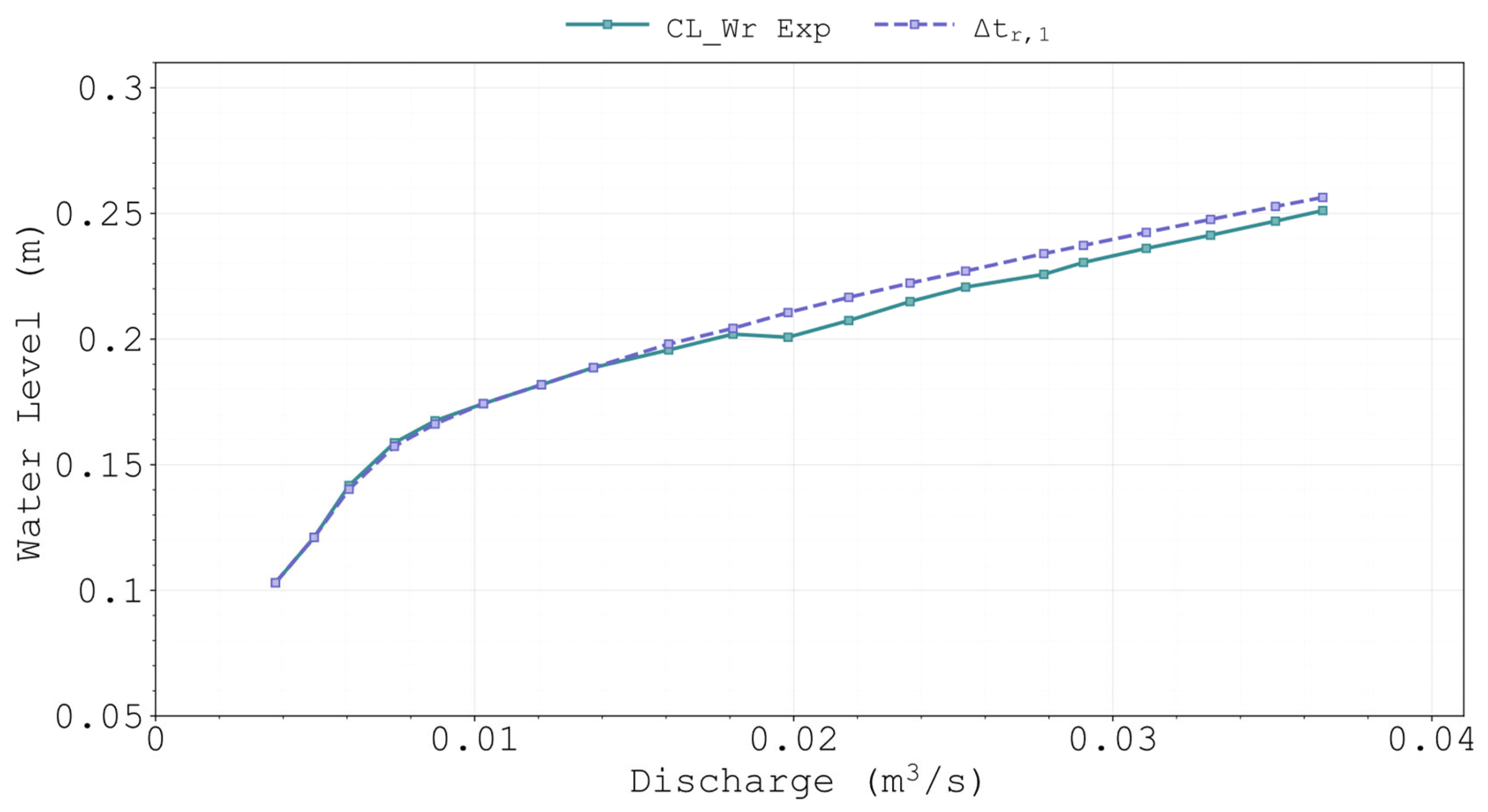
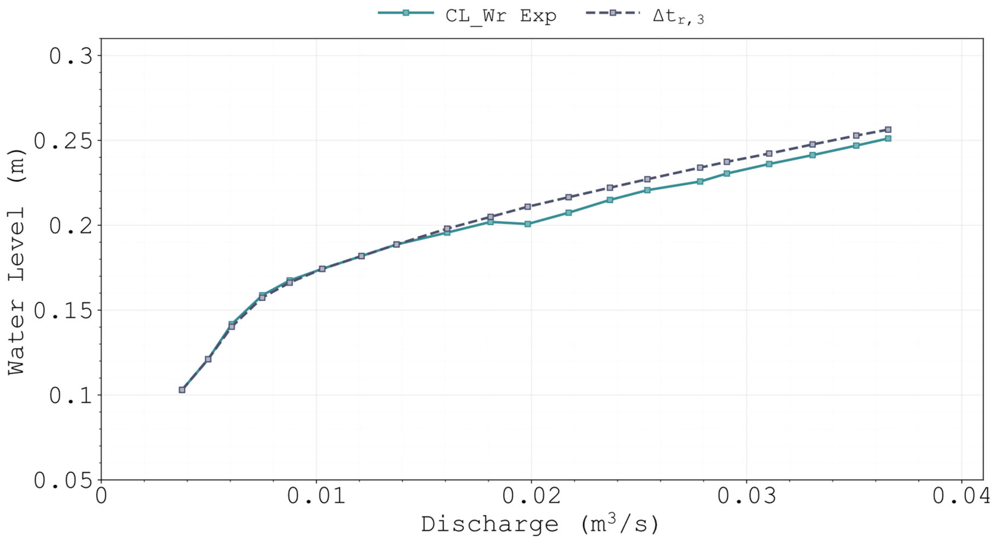
This appendix presents the individual headwater–discharge comparisons for each ramp time strategy tested in the combined culvert–weir rising limb simulations. These plots (Figure A3, Figure A4, Figure A5 and Figure A6) complement Figure 9 by separating the four numerical cases, allowing the agreement between each ramping strategy and the experimental curve to be assessed more clearly.
Figure A3. Headwater–discharge relationship for the combined culvert–weir rising limb using the fast-ramp strategy Δ t r , 1 .
Water 18 02081 g0a3
Figure A4. Headwater–discharge relationship for the combined culvert–weir rising limb using the slow ramp strategy Δ t r , 2 .
Water 18 02081 g0a4
Figure A5. Headwater–discharge relationship for the combined culvert–weir rising limb using the first hybrid ramp strategy Δ t r , 3 .
Water 18 02081 g0a5
Figure A6. Headwater–discharge relationship for the combined culvert–weir rising limb using the second hybrid ramp strategy Δ t r , 4 .
Water 18 02081 g0a6

References

  1. Schall, J.D.; Thompson, P.L.; Zerges, S.M.; Kilgore, R.T.; Morris, J.L. Hydraulic Design of Highway Culverts, 3rd ed.; Report FHWA-HIF-12-026; Hydraulic Design Series No. 5; Federal Highway Administration: Washington, DC, USA, 2012.
  2. Mile High Flood District. Urban Storm Drainage Criteria Manual, Volume 2: Structures, Storage and Recreation, Chapter 11: Culverts and Bridges; The Mile High Flood District: Lakewood, CO, USA, 2025. Available online: https://mhfd.org/files/27935c050/11_Culverts-and-Bridges.pdf (accessed on 19 August 2026).
  3. Fallowfield, L.; Motta, D. The permanent flood risk of culverts and the impact of increasing debris blockage. J. Flood Risk Manag. 2024, 17, e13021. [Google Scholar] [CrossRef] [Scilit]
  4. Jaeger, R.; Tondera, K.; Pather, S.; Porter, M.; Jacobs, C.; Tindale, N. Flow control in culverts: A performance comparison between inlet and outlet control. Water 2019, 11, 1408. [Google Scholar] [CrossRef] [Scilit]
  5. Chin, D.A. Hydraulic analysis and design of pipe culverts: USGS versus FHWA. J. Hydraul. Eng. 2013, 139, 886–893. [Google Scholar] [CrossRef] [Scilit]
  6. Meselhe, E.A.; Hebert, K. Laboratory measurements of flow through culverts. J. Hydraul. Eng. 2007, 133, 973–976. [Google Scholar] [CrossRef] [Scilit]
  7. Wasko, C.; Nathan, R.; Stein, L.; O’Shea, D. Evidence of shorter more extreme rainfalls and increased flood variability under climate change. J. Hydrol. 2021, 603, 126994. [Google Scholar] [CrossRef] [Scilit]
  8. Schütte, S.; Schulze, R.E. Projected impacts of urbanisation on hydrological resource flows: A case study within the uMngeni Catchment, South Africa. J. Environ. Manag. 2017, 196, 527–543. [Google Scholar] [CrossRef] [Scilit] [PubMed]
  9. Cullis, J.; Alton, T.; Arndt, C.; Cartwright, A.; Chang, A.; Gabriel, S.; Gebretsadik, Y.; Hartley, F.; de Jager, G.; Makrelov, K.; et al. An Uncertainty Approach to Modelling Climate Change Risk in South Africa; WIDER Working Paper 2015/045; UNU-WIDER: Helsinki, Finland, 2015. [Google Scholar] [CrossRef] [Scilit]
  10. Pozos-Estrada, O. Influence of entrapped air on hydraulic transients during rapid closure of a valve located upstream and downstream of an air pocket in pressurised pipes. Water 2025, 17, 927. [Google Scholar] [CrossRef] [Scilit]
  11. Wright, S.J.; Determan, K.V.; Vargas, S.M. Pressure transients due to compression of trapped air in rapidly filling sewer storage tunnels. J. Water Manag. Model. 2012, 20, R245-01. [Google Scholar] [CrossRef] [Scilit]
  12. Bergant, A.; Tijsseling, A.; Kim, Y.; Karadžić, U.; Zhou, L.; Lambert, M.F.; Simpson, A.R. Unsteady pressures influenced by trapped air pockets in water-filled pipelines. Stroj. Vestn.–J. Mech. Eng. 2018, 64, 501–512. [Google Scholar] [CrossRef] [Scilit]
  13. Zhou, L.; Liu, D. Experimental investigation of entrapped air pocket in a partially full water pipe. J. Hydraul. Res. 2013, 51, 469–474. [Google Scholar] [CrossRef] [Scilit]
  14. Cebe, K.; Bilhan, Ö.; Sınanmış Balcı, R. Comparative analysis of HEC-RAS, SWMM, and THDH approaches in highway culvert design. Dicle Üniversitesi Mühendis. Fakültesi Mühendis. Derg. 2024, 15, 977–992. [Google Scholar] [CrossRef] [Scilit]
  15. Conesa-García, C.; García-Lorenzo, R. Evaluating the effectiveness of road-crossing drainage culverts in ephemeral streams. Hydrol. Process. 2013, 27, 1781–1796. [Google Scholar] [CrossRef] [Scilit]
  16. Chow, V.T. Open-Channel Hydraulics; McGraw-Hill: New York, NY, USA, 1959. [Google Scholar]
  17. Horritt, M.S.; Bates, P.D. Evaluation of 1D and 2D numerical models for predicting river flood inundation. J. Hydrol. 2002, 268, 87–99. [Google Scholar] [CrossRef] [Scilit]
  18. Zeyrek, O.; Wang, F.; Xu, J. Behaviors of highway culverts subjected to flooding: A comprehensive review. Water 2025, 17, 2937. [Google Scholar] [CrossRef] [Scilit]
  19. Mark, O.; Weesakul, S.; Apirumanekul, C.; Boonya-Aroonnet, S.; Djordjević, S. Potential and limitations of 1D modelling of urban flooding. J. Hydrol. 2004, 299, 284–299. [Google Scholar] [CrossRef] [Scilit]
  20. Coutu, S.; Del Giudice, D.; Rossi, L.; Barry, D.A. Parsimonious hydrological modeling of urban sewer and river catchments. J. Hydrol. 2012, 464–465, 477–484. [Google Scholar] [CrossRef] [Scilit]
  21. Leandro, J.; Chen, A.S.; Djordjević, S.; Savić, D.A. Comparison of 1D/1D and 1D/2D coupled (sewer/surface) hydraulic models for urban flood simulation. J. Hydraul. Eng. 2009, 135, 495–504. [Google Scholar] [CrossRef] [Scilit]
  22. Trajkovic, B.; Ivetic, M.; Calomino, F.; Dippolito, A. Investigation of transition from free surface to pressurized flow in a circular pipe. Water Sci. Technol. 1999, 39, 105–112. [Google Scholar] [CrossRef] [Scilit]
  23. An, H.; Lee, S.; Noh, S.J.; Kim, Y.; Noh, J. Hybrid numerical scheme of Preissmann slot model for transient mixed flows. Water 2018, 10, 899. [Google Scholar] [CrossRef] [Scilit]
  24. Schubert, J.E.; Sanders, B.F. Building treatments for urban flood inundation models and implications for predictive skill and modeling efficiency. Adv. Water Resour. 2012, 41, 49–64. [Google Scholar] [CrossRef] [Scilit]
  25. Teng, J.; Jakeman, A.J.; Vaze, J.; Croke, B.F.W.; Dutta, D.; Kim, S. Flood inundation modelling: A review of methods, recent advances and uncertainty analysis. Environ. Model. Softw. 2017, 90, 201–216. [Google Scholar] [CrossRef] [Scilit]
  26. Jarman, D.S.; Faram, M.G.; Butler, D.; Tabor, G.; Stovin, V.R.; Burt, D.; Throp, E. Computational fluid dynamics as a tool for urban drainage system analysis: A review of applications and best practice. In Proceedings of the 11th International Conference on Urban Drainage (ICUD), Edinburgh, UK, 31 August–5 September 2008. [Google Scholar]
  27. Olsen, N.R.B.; Kjellesvig, H.M. Three-dimensional numerical flow modeling for estimation of maximum local scour depth. J. Hydraul. Res. 1998, 36, 579–590. [Google Scholar] [CrossRef] [Scilit]
  28. Zeng, J.; Rakib, Z.; Ansar, M.; Hajimirzaie, S.; Chen, Z. Application of hybrid flow data and dimensional analysis to gated-culvert flow estimation. J. Irrig. Drain. Eng. 2020, 146, 04020026. [Google Scholar] [CrossRef] [Scilit]
  29. Zhang, R.; Jin, Y.-C.; Wu, P. Numerical simulation of culvert flow using OpenFOAM. In Proceedings of the 38th IAHR World Congress, Panama City, Panama, 1–6 September 2019. [Google Scholar] [CrossRef] [Scilit]
  30. van Vliet, J. Improving Culvert Performance: Reducing Energy Losses by Streamlining the Entrance and Exit of Culverts. Master’s Thesis, Delft University of Technology, Delft, The Netherlands, 2024. Available online: https://resolver.tudelft.nl/uuid:e5bebc6d-f3de-4155-959e-423f3cefbb9c (accessed on 19 August 2026).
  31. Le, H.T.T.; Nguyen, C.V.; Le, D.-H. Numerical study of sediment scour at meander flume outlet of boxed culvert diversion work. PLoS ONE 2022, 17, e0275347. [Google Scholar] [CrossRef] [Scilit] [PubMed]
  32. Mostafazadeh-Fard, S.; Samani, Z. Dissipating culvert end design for erosion control using CFD platform FLOW-3D numerical simulation modeling. J. Pipeline Syst. Eng. Pract. 2023, 14, 04022064. [Google Scholar] [CrossRef] [Scilit]
  33. Ahmed, K.O.; Kavianpour, M.R.; Amini, A.; Aminpour, Y. Numerical modelling of downstream scour in circular culverts: Impact of inlet blockages and variable flow conditions. PLoS ONE 2024, 19, e0312501. [Google Scholar] [CrossRef] [Scilit] [PubMed]
  34. Sorourian, S. Turbulent flow characteristics at the outlet of partially blocked box culverts. In Proceedings of the 36th IAHR World Congress, The Hague, The Netherlands, 28 June–3 July 2015. [Google Scholar]
  35. Sorourian, S.; Keshavarzi, A.; Ball, J.E. Scour at partially blocked box-culverts under steady flow. Proc. Inst. Civ. Eng. Water Manag. 2016, 169, 247–259. [Google Scholar] [CrossRef] [Scilit]
  36. Taha, N.; El-Feky, M.M.; El-Saiad, A.A.; Fathy, I. Numerical investigation of scour characteristics downstream of blocked culverts. Alex. Eng. J. 2020, 59, 3503–3513. [Google Scholar] [CrossRef] [Scilit]
  37. Crispino, G.; Dorthe, D.; Gisonni, C.; Pfister, M. Hydraulic capacity of bend manholes for supercritical flow. J. Irrig. Drain. Eng. 2023, 149, 04022048. [Google Scholar] [CrossRef] [Scilit]
  38. Crispino, G.; Maietta, F.; Iervolino, M.; Gisonni, C. Numerical study on a supercritical vortex drop shaft with a spiral inlet. Results Eng. 2025, 25, 104197. [Google Scholar] [CrossRef] [Scilit]
  39. Hirt, C.W.; Nichols, B.D. Volume of fluid (VOF) method for the dynamics of free boundaries. J. Comput. Phys. 1981, 39, 201–225. [Google Scholar] [CrossRef] [Scilit]
  40. Liu, X.; Chen, Q.-S.; Zeng, Z.-N.; Dong, Z. Optimisation of bridge pier winding flow numerical simulation scheme based on Delft3D. Water 2024, 16, 2079. [Google Scholar] [CrossRef] [Scilit]
  41. Park, J.-C.; Kim, M.-H.; Miyata, H.; Chun, H.-H. Fully nonlinear numerical wave tank (NWT) simulations and wave run-up prediction around 3-D structures. Ocean Eng. 2003, 30, 1969–1996. [Google Scholar] [CrossRef] [Scilit]
  42. Tang, P.; Lin, X.; Wang, W.; Zhang, H. Numerical simulation of hydrodynamic performance of an offshore oscillating water column wave energy converter device. J. Mar. Sci. Eng. 2024, 12, 2289. [Google Scholar] [CrossRef] [Scilit]
  43. Legendre, A.-M. Nouvelles Méthodes Pour la Détermination des Orbites des Comètes; Firmin Didot: Paris, France, 1805. [Google Scholar]
  44. Stigler, S.M. Gauss and the invention of least squares. Ann. Stat. 1981, 9, 465–474. [Google Scholar] [CrossRef] [Scilit]
  45. Boscovich, R.J. De Litteraria Expeditione per Pontificiam Ditionem. Bononiensi Sci. Artium Inst. Atque Acad. Comment. 1757, 4, 353–396. [Google Scholar]
  46. Koenker, R.; Bassett, G. On Boscovich’s estimator. Ann. Stat. 1985, 13, 1625–1628. [Google Scholar] [CrossRef] [Scilit]
  47. Wright, S. Correlation and causation. J. Agric. Res. 1921, 20, 557–585. [Google Scholar]
  48. Legates, D.R.; McCabe, G.J. Evaluating the use of “goodness-of-fit” measures in hydrologic and hydroclimatic model validation. Water Resour. Res. 1999, 35, 233–241. [Google Scholar] [CrossRef] [Scilit]
  49. Moriasi, D.N.; Arnold, J.G.; Van Liew, M.W.; Bingner, R.L.; Harmel, R.D.; Veith, T.L. Model evaluation guidelines for systematic quantification of accuracy in watershed simulations. Trans. ASABE 2007, 50, 885–900. [Google Scholar] [CrossRef] [Scilit]
  50. Chen, Y.; Li, P.; Fei, Z.; Wang, R.; Zhang, H.; Zhu, D.Z.; Qian, S. Air–water interactions during rapid filling of a closed horizontal pipe. Phys. Fluids 2025, 37, 043326. [Google Scholar] [CrossRef] [Scilit]
  51. Hu, Y.; Wang, D.; Liu, S.; Xu, Y.; Zhou, L. Experimental study of mixed flow transitions in pipes with air pocket effects. Phys. Fluids 2025, 37, 114116. [Google Scholar] [CrossRef] [Scilit]
Figure 1. The 3D computational geometry (grey) and block-structured mesh (blue lines): (a) full-flume domain; (b) culvert–weir configuration; (c) culvert-only configuration; and (d) weir-only configuration.
Water 18 02081 g001
Figure 2. Boundary conditions: (a) side view; (b) front view.
Water 18 02081 g002
Figure 3. Rising limbs of culvert-only, weir-only and culvert–weir combined configurations. The grey zone (A) highlights the culvert-only portion of the plot analyzed further in Section 4.2.2.
Water 18 02081 g003
Figure 4. Receding limbs of culvert-only and culvert–weir configurations.
Water 18 02081 g004
Figure 5. Mesh sensitivity comparison for the benchmark culvert–weir geometry. In the fluid-fraction contours, red denotes water ( F = 1 ), blue denotes air/void ( F = 0 ), intermediate colors denote the free-surface interface, and grey denotes solid geometry.
Water 18 02081 g005
Figure 6. Wall shear stress and streamlines at the culvert inlet edge: (a) benchmark mesh; (b) refined mesh. Zoomed view shown without streamlines for clarity.
Water 18 02081 g006
Figure 7. Rising limb of culvert-only configuration after mesh refinement. Corresponding to region A in Figure 3.
Water 18 02081 g007
Figure 8. Velocity magnitude contours on a 2D centerline slice of the first culvert barrel showing the effect of inflow ramping strategy on outlet attachment, ventilation and culvert flow regime: (a) Δ t r , 1 ; (b) Δ t r , 2 ; (c) Δ t r , 3 ; and (d) Δ t r , 4 . Grey regions represent solid geometry and white regions represent air.
Water 18 02081 g008
Figure 9. Water level–discharge relationship obtained with different ramp times compared with the experiment.
Water 18 02081 g009
Figure 10. Hydraulic behavior comparison of turbulence model: (a) RNG; (b) LES; (c) k ε ; (d) kw. black arrowsindicates regions of incomplete barrel filling and white dots delineate air pockets.
Water 18 02081 g010
Figure 11. Wall shear stress comparison of turbulence model: (a) RNG; (b) LES; (c) k ε ; (d) kw.
Water 18 02081 g011
Figure 12. Unsteady state free flow, experiment vs. CFD: (a) Full measurements; (b) upstream ( h 1 ); (c) Above the weir ( h 4 ); (d) Downstream ( h 5 ).
Water 18 02081 g012
Table 1. Summary of experimental validation and numerical sensitivity cases.
(a) Validation Cases
IDCaseQ (L/s)/Levels Δ t r / Δ t p Model/MeshOutputs
V1Culvert–weir, steady rising3.758–36.581; 205 s/60 sRNG k–ε; benchmark mesh h 1 ; h Q ; submergence; overtopping; barrel filling; ventilation.
V2Weir-only, steady rising4.991–29.418; 105 s/60 sRNG k–ε; benchmark mesh h 1 ; h Q ; overtopping
V3Culvert-only, steady rising3.106–11.740; 175 s/60 sRNG k–ε; benchmark mesh h 1 ; h Q ; submergence; barrel state.
V4Culvert–weir, steady receding36.581–3.758; 205 s/60 sRNG k–ε; benchmark mesh h 1 ; recession response; barrel state
V5Culvert-only, steady receding15.040–2.769; 195 s/60 sRNG k–ε; benchmark mesh h 1 ; h Q ; full-to-partial transition
V6Culvert–weir, continuous unsteady hydrograph2 → 30 → 2/continuous hydrograph -RNG k–ε; benchmark mesh h 1 , h 4 , h 5 ; Stage evolution; peak stage/time; regime transition
(b) Additional Numerical Analyses
AnalysisQ (L/s)/LevelsVariants Δ t r / Δ t p Model/MeshOutputs
Local inlet refinement, applied to V33.106–11.740; 17 Benchmark; refined inlet5 s/60 sRNG k–ε, 0.09D; RNG k–ε, 0.02D h 1 ; streamlines; WSS.
Ramp time sensitivity, applied to V13.758–36.581; 20 Δ t r , 1 ; Δ t r , 2 ; Δ t r , 3 ;   Δ t r , 4 -/60 s:
5/60; 60/60; 5 → 60 → 5/60; 60 → 5/60
RNG k–ε; benchmark mesh, h 1 ; outlet state; ventilation; air-pocket; barrel filling
Turbulence-model sensitivity, applied to V13.758–36.581; 20 RNG k–ε;
Standard k–ε; k–w;
LES
5 s/60 sBenchmark mesh h 1 ; barrel filling; air-pocket; WSS
Additional physics trials, applied to V13.758–36.581; 20 Baseline; ST 1; AE 2; ST + AE5 s/60 sRNG k–ε; benchmark mesh h 1 ; h Q
Full-geometry mesh verificationV1; V17 meshes; 0.28D–0.08D5 s/60 sRNG k–ε h 1 ; barrel state; cells; runtime
Notes: 1 Surface tension; 2 air entrainment.
Table 2. Fine-mesh convergence of upstream water level h 1 .
Mesh PairMean Rel. Diff. (%)Max Rel. Diff. (%)Mean | Δ h 1 | (mm)Max | Δ h 1 | (mm)Cost Increase
0.10D → 0.09D0.472.240.783.18+26.9% cells; +73.2% runtime
0.09D → 0.08D0.170.350.340.86+35.9% cells; +71.5% runtime
Table 3. Inlet region mesh refinement.
CaseInlet Cell SizeWSS EffectHeadwater Response
Benchmark0.09 D Lower WSSUnderpredicted post-submergence headwater
Refined0.02 D Upper-edge WSS ~ 2–3 × higherCloser post-submergence h Q agreement
Table 4. Summary of ramp history cases and hydraulic outcomes.
CaseRamp History t r * Γ × 10 3 RegimeOutlet State
Δ t r , 1 Fast 5 s, all steps56.733.851–8.608No transitionDetached/Ventilated
Δ t r , 2 Slow 60 s, all steps680.780.321–0.717Early transitionAttached/Sealed
Δ t r , 3 Hybrid 5–60–5 s56.73–680.780.321–8.268No transitionAttached → ventilated
Δ t r , 4 Hybrid 60–5 s56.73–680.780.363–6.399Early transitionLater ventilation
Table 5. Turbulence model sensitivity.
Turbulence ModelBarrel FillingAir-Pocket ExtentWSSEffect on h 1
RNG k ε HighestSmallestRelatively uniformNegligible
LESLower than RNGModerateLow, spatially variableNegligible
Standard k ε Lower than LESLargerRelatively uniformNegligible
k w LowestLargestSharp local inlet peaksNegligible
Table 6. Statistical metrics: experiment vs. CFD.
CaseRMSE (mm)MAE (mm)R2MARE (%)
Weir-only (rising)2.152.120.99340.90
Culvert-only (rising)10.137.270.97473.21
Culvert–weir (rising) Δ t r , 1 5.253.960.98311.84
Culvert–weir (receding) Δ t r , 1 10.969.530.93825.42
Table 7. Quantitative comparison for the unsteady culvert–weir case.
LocationRMSE (mm)MAE (mm) R 2 Peak Stage Err. (mm)Peak Time Err. (s)
h19.356.340.97765.612.25
h43.022.200.81357.70.26
Table 8. Dimensionless ranges characterizing the investigated hydraulic conditions.
ConfigurationSource h Q F r R e
Unsteady culvert–weirExperiment0.501–3.0280.542–5.4820.074–0.142 1.81 × 10 4 1.12 × 10 5
Unsteady culvert–weirCFD0.540–3.0940.563–5.4750.073–0.136 1.83 × 10 4 1.10 × 10 5
Steady culvert–weirExperiment0.785–2.7290.749–7.2870.083–0.212 2.33 × 10 4 1.56 × 10 5
Steady culvert–weirCFD0.785–2.7970.749–7.2870.083–0.205 2.33 × 10 4 1.54 × 10 5
Steady weir-onlyExperiment1.905–3.0220.994–5.8600.045–0.150 2.45 × 10 4 1.19 × 10 5
Steady weir-onlyCFD1.926–3.0510.994–5.8600.044–0.148 2.44 × 10 4 1.19 × 10 5
Steady culvert-onlyExperiment0.531–3.3040.619–2.3390.053–0.094 2.05 × 10 4 4.57 × 10 4
Steady culvert-onlyCFD0.531–3.1330.619–2.3390.057–0.094 2.05 × 10 4 4.71 × 10 4
Disclaimer/Publisher’s Note: The statements, opinions and data contained in all publications are solely those of the individual author(s) and contributor(s) and not of MDPI and/or the editor(s). MDPI and/or the editor(s) disclaim responsibility for any injury to people or property resulting from any ideas, methods, instructions or products referred to in the content.