Depth-Ratio Effects on Flow in a Partially Vegetated Compound Channel

Abstract

Laboratory experiments were conducted to investigate the effects of the relative depth ratio, $D_r$, on flow in an asymmetric compound channel with a partially vegetated floodplain. Five cases covering $D_r=0.15-0.52$ were examined. Partial-width vegetation produced two lateral shear layers: the main-channel/floodplain (MCFP) layer and the non-vegetated/vegetated-floodplain (NVV) layer. As $D_r$ increased, streamwise velocity and discharge were redistributed from the main channel toward the floodplain: the main-channel discharge fraction decreased from 83.7% to 56.6%, while the combined floodplain fraction increased from 16.31% to 43.33%. The dimensionless shear parameters ${\lambda }_{MCFP}$ and ${\lambda }_{NVV}$ decreased from 0.584 to 0.064 and from 0.741 to 0.316, respectively, with ${\lambda }_{NVV}>{\lambda }_{MCFP}$ in all cases. The maximum local Reynolds shear stress occurred near the NVV interface. For the four cases measured using an acoustic Doppler velocimeter (ADV), mean transverse advection dominated the total depth-averaged transverse momentum exchange, and its case-wise maximum magnitude exceeded those of the Reynolds-stress and dispersive contributions by factors of 71.4–356.3 and 74.2–556.7, respectively. Spectral analysis indicated that large-scale coherent motions over the floodplain were strongest under shallow-flow conditions and weakened as $D_r$ increased. These findings show that $D_r$ regulates the relative roles of the two shear layers.

1. Introduction

Natural rivers often exhibit compound-channel cross-sections with partially vegetated floodplains. In partially vegetated compound channels, patchy vegetation introduces pronounced spanwise variations in vegetation drag and hydraulic roughness, resulting in velocity distributions that differ from those in fully vegetated or non-vegetated compound channels [1,2,3,4,5]. Under overbank-flow conditions, the abrupt bed elevation change at the main-channel/floodplain (MCFP) interface and the vegetation-drag discontinuity at the non-vegetated/vegetated (NVV) floodplain interface produce two coexisting lateral shear layers. The coexistence of these shear layers may produce coupled effects on velocity redistribution, coherent structures, and momentum exchange. The strength and spatial extent of each shear layer depend on the velocity contrast across its corresponding interface. The MCFP velocity contrast is strongly affected by the relative depth ratio, $D_r=h/H$, where $h$ and $H$ denote the water depths in the floodplain and the main channel, respectively [6], whereas the NVV velocity contrast is associated with vegetation-induced drag and flow redistribution [7]. However, how variations in $D_r$ modify the relative strengths of the two shear layers in a partially vegetated compound channel remains unclear. Understanding how $D_r$ affects velocity distributions, shear layer characteristics, coherent structures, and momentum exchange is therefore important for characterizing flow structure in partially vegetated compound channels.

Previous studies have shown that $D_r$ alters the velocity difference between the main channel (MC) and the floodplain (FP) and thereby affects the development of the MCFP shear layer, coherent structures, and transverse momentum exchange [8,9,10,11]. For uniform compound channel flows, existing $D_r$-based classifications indicate that shallow overbank flows, such as $D_r$ < 0.33, are commonly associated with monotonic velocity profiles and clockwise-rotating macro-vortices near the MCFP interface [9,12,13]. At intermediate depth ratios, such as 0.33 < $D_r$ < 0.5, non-monotonic velocity profiles and a velocity dip near the MCFP interface have been reported, indicating the presence of counter-rotating macro-vortices [9,12,13]. At larger depth ratios, such as $D_r$ > 0.5, non-monotonic profiles may still occur, but the shear in the transition region tends to weaken, resulting in lower Reynolds shear stresses than those observed under shallower conditions [8,9,12]. Although the exact threshold values vary with channel geometry, roughness, and flow conditions [8,9,10,14], these classifications indicate that the response of the transverse shear layer to $D_r$ is complex and not necessarily monotonic.

The complex response of shear-layer turbulence to $D_r$ can be attributed to two competing effects of relative depth. First, decreasing $D_r$ strengthens the topographical forcing associated with the two-stage geometry. This forcing can sustain shear-layer turbulence [15], while the cross-stream change in flow depth can generate quasi-two-dimensional macro vortices in uniform compound-channel flows [12,16]. Second, a decrease in floodplain water depth increases the vertical confinement of the shear layer, which reduces the peak magnitude of the depth-averaged Reynolds stress and limits the transverse extent of turbulent lateral shear [12]. This constraining effect is weaker when turbulence is organized into quasi-two-dimensional structures, indicating that the influence of $D_r$ depends jointly on vertical confinement and interfacial shear [12].

Consistent with these competing effects, previous studies have shown that relative depth affects the magnitude and transverse development of MCFP shear-layer turbulence through vertical confinement, whereas the formation of quasi-two-dimensional coherent structures is governed more directly by interfacial shear and the direction and magnitude of the mean transverse flow [12]. Under uniform-flow conditions, shear-layer turbulence generally decreases as $D_r$ increases [12]. However, the range of $D_r$ over which LHCSs form or persist appears to differ among vegetation configurations. In non-vegetated compound channels, coherent structures have been reported to diminish when $D_r>0.25$ [12,17], whereas studies under fully vegetated [18] and partially vegetated floodplain conditions [19] indicate that LHCSs may persist at higher depth ratios, such as $D_r=0.4$–0.5.

These contrasting observations suggest that $D_r$ alone may not fully characterize the interfacial shear conditions controlling LHCSs formation. To characterize the velocity contrast across the MCFP mixing layer more directly, the dimensionless shear parameter is expressed here, following Proust, Fernandes, Leal, Rivière and Peltier [12], as:

$${\lambda }_{MCFP}={\displaystyle \frac{U_1-U_2}{U_1+U_2}}$$

(1)

where $U_1$ and $U_2$ are the streamwise depth-averaged velocities of the ambient flows outside the MCFP mixing layer on the MC and FP sides, respectively. Related experiments on shallow mixing layers by Proust et al. [20] further demonstrated the importance of the shear parameter in controlling mixing-layer characteristics. In the present partially vegetated configuration, $U_2$ corresponds to the streamwise depth-averaged velocity in the non-vegetated floodplain region between the MCFP and NVV mixing layers. The dimensionless shear parameter affects the width and structure of the MCFP mixing layer and therefore influences the conditions under which LHCSs form. Because vegetation can modify the velocity difference between the MC and FP, it may alter ${\lambda }_{MCFP}$ at a given $D_r$ [6,14]. This may partly explain why the $D_r$ range associated with LHCSs formation or persistence differs among non-vegetated, fully vegetated, and partially vegetated compound channels. However, ${\lambda }_{MCFP}$ characterizes only the velocity contrast across the MCFP interface and does not represent the additional NVV shear layer present in partially vegetated compound channels. Therefore, it is essential to employ a similar shear parameter to characterize the velocity contrast across the NVV interface (see Section 3).

Although LHCSs contribute to the transverse exchange of streamwise momentum through Reynolds stresses, the total depth-averaged exchange also includes transverse-advection and dispersive-stress contributions. Following Proust, Fernandes, Leal, Rivière and Peltier [12], the depth-averaged transverse exchange of streamwise momentum can be decomposed into three main contributions: the depth-averaged Reynolds-stress contribution, the transverse-advection contribution associated with the depth-averaged mean transverse flow, and the dispersive-stress contribution associated with secondary currents. The relative importance of these contributions depends strongly on the direction and magnitude of the mean transverse flow. When a strong transverse flow is directed toward the MC, the transverse-advection contribution can dominate the momentum exchange, whereas Reynolds stress, transverse advection, and dispersive stress can all contribute when the transverse flow is directed toward the FP [12]. Recent experiments in a compound channel with a heterogeneous floodplain forest showed that vegetation-induced flow readjustment generated a strong mean transverse flow from the FP toward the MC; the associated transverse-advection contribution accounted for more than 95% of the total momentum exchange at the mixing-layer center [14]. However, it remains unclear how partial-width vegetation modifies the mean transverse flow and how its contribution to the total transverse momentum exchange varies with $D_r$, particularly when the MCFP and NVV shear layers coexist.

The secondary-current-related dispersive contribution can also be important. Dupuis, Proust, Berni and Paquier [6] found that this contribution was of the same order of magnitude as the Reynolds-stress contribution within the MC but was negligible at the MCFP interface, indicating that secondary currents primarily redistributed streamwise momentum within the MC rather than directly between the MC and FP. Proust, Fernandes, Leal, Rivière and Peltier [12] further showed that vertical confinement can constrain the transverse development of shear-layer turbulence and reduce peak Reynolds stresses, particularly under weakly sheared conditions dominated by three-dimensional turbulence. These findings motivate examining whether variations in $D_r$ alter the balance among the three momentum-exchange contributions in partially vegetated compound channels.

Although some previous studies have examined aspects of velocity distribution, coherent structures, and transverse momentum exchange in partially vegetated compound channels [19,21,22], the dependence of these processes on $D_r$ remains insufficiently resolved. Existing $D_r$-based flow-regime classifications have been developed mainly for non-vegetated compound channels, while available dimensionless-shear relationships generally describe a single dominant mixing layer. Their applicability to partially vegetated compound channels, where the MCFP and NVV shear layers coexist, therefore remains uncertain. In particular, it remains unclear how variations in $D_r$ alter the relative strengths and interaction of the two shear layers, how LHCS formation and persistence differ between the MCFP and NVV interfaces, and how the relative contributions of Reynolds stress, transverse advection, and dispersive stress to the total transverse momentum exchange vary with $D_r$. These unresolved issues collectively define the principal knowledge gap addressed in the present study.

Therefore, this study investigates how the relative depth ratio $D_r$ modulates flow structure and transverse momentum exchange in a partially vegetated compound channel. Laboratory experiments were conducted over a range of $D_r$ values to: (i) characterize the resulting changes in velocity distributions and in the relative strengths of the MCFP and NVV shear layers; (ii) examine how $D_r$ affects the formation and persistence of LHCSs at the two interfaces; and (iii) quantify the relative contributions of Reynolds stress, transverse advection, and dispersive stress to the total transverse momentum exchange. The results provide process-level understanding of depth ratio-dependent flow organization in partially vegetated compound channels and a hydraulic basis for improving the representation of velocity redistribution and lateral momentum exchange in compound-channel models.

This paper is structured as follows: Section 2 describes the apparatus, flow conditions, and measurement techniques. Section 3 outlines the data analysis methods. Section 4 presents experimental results and discussion on velocity distributions, transverse momentum exchange, and turbulent structures. Finally, the key findings and conclusions are summarized in Section 5.

2. Experimental Setup

2.1. Experimental Apparatus

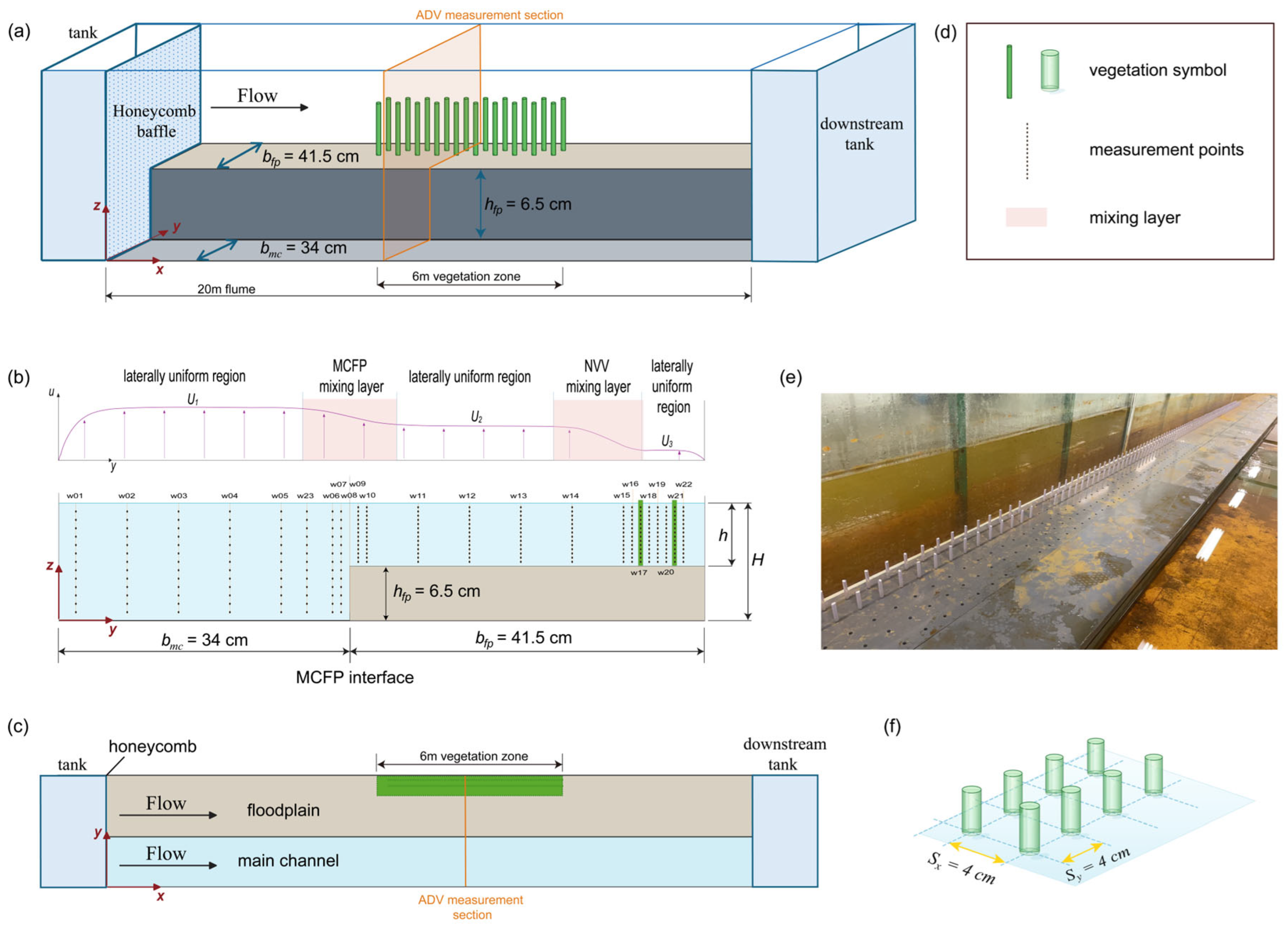
The experiments were conducted in a water flume at the hydraulic laboratory of Xi’an Jiaotong-Liverpool University. The flume is 0.755 m wide, 20 m long, and 0.8 m deep with a 6 m-long vegetation zone starting from x = 8 m (see Figure 1). The x, y, and z refer to the longitudinal (positive downstream), transverse (positive towards the floodplain wall), and vertical (positive upwards) directions, respectively. Under this coordinate system, x = 0 indicates the inlet cross-section; y = 0 indicates the flume wall of the main channel; z = 0 indicates the flume bed of the main channel. The flume bed and walls are made of painted steel and plexiglass, respectively, with a fixed bed slope of 0.003. The floodplain was constructed with PVC boards, with a width $b_{fp}$ = 41.5 cm and a height $h_{fp}$ = 6.5 cm (the subscript fp denotes the floodplain).

Plastic dowels were used to simulate rigid vegetation, with a diameter d of 6.35 mm as suggested by Van Rooijen et al. [23] and a height h_v of 4 cm. The distance between the neighboring dowels in the x and y directions is 4 cm, i.e., $S_x=S_y=$ 4 cm, where $S_x$ and $S_y$ are the vegetation spacing in the x and y directions, respectively.

2.2. Flow Conditions

All test cases were conducted under streamwise quasi-uniform and steady conditions. A honeycomb baffle was placed at the beginning of the flume to reduce turbulence and non-uniformity (Figure 1). Despite the difficulty in achieving strictly uniform flows, we assume that if local water depth D at the lateral position y, $D\left(y\right)$, in the vegetated region (the region between x = 8 m and x = 14 m) remains constant, i.e., ${\displaystyle \frac{\partial D\left(y\right)}{\partial x}}={\displaystyle \frac{\partial z_b}{\partial x}}$ ($z_b$ refers to the z position of the flume bottom), the flow could be considered streamwise uniform flow in this region. This method has also been adopted by Van Prooijen et al. [24], Dorcheh [25], Hamidifar et al. [26], and Proust and Nikora [10].

The channel Reynolds number $Re$ and the stem Reynolds number ${Re}_d$, the channel Froude number $Fr$ and the stem Froude number ${Fr}_d$ were used to characterize the flow condition, which are defined by Equations (2) and (3), respectively. The details of the test parameters are summarized in

Table 1. Summary of Experiments.

Case	H (cm)	$\mathit{h}$ (cm)	${\mathit{D}}_{\mathit{r}}$	${\mathit{U}}_0$ (cm/s)	$\mathit{R}\mathit{e}$	${\mathit{R}\mathit{e}}_{\mathit{d}}$	$\mathit{F}\mathit{r}$	${\mathit{F}\mathit{r}}_{\mathit{d}}$	Measurement
1	7.6	1.1	0.15	50.85	16978	82	0.89	0.04	propeller
2	8.8	2.3	0.26	50.20	21195	498	0.78	0.17	ADV
3	9.6	3.1	0.32	54.65	26156	617	0.80	0.18	ADV
4	11	4.5	0.41	46.70	26751	706	0.62	0.17	ADV
5	13.6	7.1	0.52	55.34	40631	1420	0.65	0.27	ADV

, covering a depth ratio $D_r$ varying between 0.15 and 0.52. In all cases, the flow was fully turbulent with a minimum $Re\approx \mathrm{16,978}$ and was subcritical with a maximum $Fr=0.89$.

$$Re={\displaystyle \frac{U_0{R}_L}{\nu }},{Re}_d={\displaystyle \frac{U_{veg}d}{\nu }}$$

(2)

$$Fr={\displaystyle \frac{U_0}{\sqrt{g{R}_L}}},{Fr}_d={\displaystyle \frac{U_{veg}}{\sqrt{gh}}}$$

(3)

where $R_L$ is the hydraulic radius, defined as $R_L=A/P$; $A$ is the total wetted cross-sectional area; $P$ is the corresponding wetted perimeter; $U_0$ is the mean channel velocity; $U_{veg}$ is the mean streamwise velocity in the vegetated zone; $\nu$ is the kinematic viscosity of water, taken as $1.004\times {10}^{-6} {\mathrm{m}}^2/\mathrm{s}$; g is the local gravitational acceleration.

2.3. Velocity and Water Level Measurements

A three-dimensional Nortek acoustic Doppler velocimeter (ADV) was used to measure the three velocity components in cases 2–5, whereas a micro-propeller velocity meter was used to measure the streamwise velocity in Case 1. According to the Nortek velocimeter manual [27], a factory-calibrated ADV has a velocity scale-factor bias of less than 1% of the measured velocity, provided that the probe geometry remains undeformed. This specification represents systematic scale-factor bias rather than the short-term uncertainty of an individual velocity sample. The latter depends on the selected velocity range, probe geometry, acoustic scattering conditions, signal-to-noise ratio (SNR), turbulence intensity, and number of samples used for averaging. The micro-propeller meter had an accuracy of 95%, and a resolution of 0.1 cm/s.

At each measuring position, the ADV data were acquired at a sampling frequency of 200 Hz for 120–180 s, corresponding nominally to 24,000–36,000 raw samples. The ADV records were processed using WinADV version 2.028. Velocity spikes were detected and removed using the robust phase-space-thresholding procedure developed by Goring and Nikora [28] and subsequently modified by Wahl [29]. Samples with correlations below 70% or SNR values below 15 dB were excluded. These thresholds are consistent with the recommendations for instantaneous velocity and turbulence measurements given by Wahl [29]. and the Nortek manual [27]. The velocity range was selected to avoid phase wrapping and velocity ambiguity.

After quality screening, the removal of invalid samples resulted in non-equidistant time series. For the power spectral density analysis presented in Section 4.4, the quality-controlled records were therefore linearly resampled onto a uniform 150 Hz time grid using MATLAB R2022a. The resampled records were used only for spectral analysis; the mean velocities and turbulence statistics were calculated from the quality-controlled ADV records before temporal resampling.

For Case 1, the micro-propeller measurements were acquired for 40 s at each position and repeated twice. The two time-averaged measurements were averaged, and their difference was used to evaluate measurement repeatability. The repeated measurements do not replace the manufacturer-specified instrument accuracy but provide an additional assessment of the reproducibility of the measured mean streamwise velocity. Because the micro-propeller meter measured only the streamwise velocity component, Case 1 was not included in the analyses of transverse velocity, Reynolds stress, dispersive stress, or the complete transverse momentum-exchange decomposition.

All velocity measurements were conducted at x = 11 m, corresponding to the y-z cross-section at the center of the 6 m long vegetated reach. This section was located 3 m downstream of the leading edge of the vegetation. Zampiron [30] suggested that an adjustment length of approximately 50–70 times the water depth may be required in conventional channels, whereas Proust and Nikora [10] reported that approximately 30 water depths may be sufficient in vegetated compound channels. On this basis, the section at x = 11 m was selected to represent approximately streamwise quasi-uniform mean-flow conditions. This assumption applies to the mean-flow field and does not imply exact longitudinal invariance of all turbulence statistics.

The lateral and vertical positions of the measuring points are summarized in

Table 2. Positions of Measurement Points.

Main Channel		Non-Vegetated Floodplain		Vegetated Floodplain
Point	y Position (cm)	Point	y Position (cm)	Point	y Position (cm)
w01	2	w08	34	w15	66
w02	8	w09	35	w16	67
w03	14	w10	36	w17	68
w04	20	w11	42	w18	69
w05	26	w12	48	w19	70
w23	29	w13	54	w20	71
w06	32	w14	60	w21	72
w07	33			w22	73

and illustrated in Figure 1. The lowest measuring elevation was 0.5 cm above the local bed for the ADV measurements and 1.0 cm above the local bed for the micro-propeller measurements. The vertical spacing between adjacent measuring points was 0.5–1.0 cm in the main channel and 0.5 cm on the floodplain.

The water-surface elevation was measured using a point gauge at the measurement cross-section x = 11 m. The total discharge was measured using an electromagnetic flowmeter installed in the inlet pipe. The flowmeter was calibrated against the time-averaged volume of water passing through the pipe.

3. Analysis Method

3.1. Velocity and Shear Layer Characterization

The lateral and vertical distributions of streamwise velocity are analyzed using the normalized velocity $U_d/U_0$, where $U_0$ is the mean channel velocity. The depth-averaged form of a quantity $\varphi$ at the lateral position $y$ is defined as:

$${\varphi }_d\left(y\right)={\displaystyle \frac{1}{D\left(y\right)}}{\int }_{z=0}^{z=D\left(y\right)}\varphi \left(y,z\right)dz$$

(4)

$$U_0=Q/A$$

(5)

where $D\left(y\right)$ is the local water depth; $Q$ is the total discharge, defined as $Q=Q_{\mathrm{M}\mathrm{C}}+Q_{\mathrm{F}\mathrm{P}}=Q_{\mathrm{M}\mathrm{C}}+Q_{\mathrm{N}\mathrm{V}\mathrm{F}\mathrm{P}}+Q_{\mathrm{V}\mathrm{F}\mathrm{P}}$; $A$ is the total wetted cross-sectional area.

The spatial structure of lateral shear layers in vegetated flows is characterized using three parameters: the dimensionless shear $\lambda$, the nominal shear layer thickness $t$, and the momentum thickness $\theta$ [12,31,32,33]. The dimensionless shear $\lambda$ (see Equation (6)) quantifies the relative magnitude of the shear between the two adjacent ambient flow regions to the convection velocity $U_c$. The nominal shear layer thickness $t$ (see Equation (7)) represents the geometric width of the region over which coherent vortices, induced by K-H instabilities, develop. The momentum thickness $\theta$ (see Equation (8)) is a theoretical length scale that measures the reduction in momentum flux due to the shear layer.

$${\lambda }_{MCFP}={\displaystyle \frac{U_1-U_2}{U_1+U_2}}, {\lambda }_{NVV}={\displaystyle \frac{U_2-U_3}{U_2+U_3}}$$

(6)

Here, ${\lambda }_{MCFP}$ quantifies the shear within the MCFP mixing layer, and ${\lambda }_{NVV}$ quantifies the shear within the NVV mixing layer.

The velocities $U_1$, $U_2$ and $U_3$ are the depth-averaged streamwise velocities representative of three ambient flow regions outside the mixing layers (Figure 1):

• $U_1$: The streamwise depth-averaged velocity of the ambient streams outside the MCFP mixing layer in the main channel. It is obtained from the approximately constant velocity observed in the main channel region.
• $U_2$: The streamwise depth-averaged velocity in the non-vegetated floodplain, situated between the MCFP and NVV mixing layers. It is derived from the nearly constant value on the non-vegetated floodplain.
• $U_3$: The streamwise depth-averaged velocity of the ambient streams within the vegetated floodplain region. $U_3$ is obtained by laterally averaging the depth-averaged velocity over the vegetated region [31].

As suggested by Caroppi, Vastila, Jarvela, Rowinski and Giugni [31], the interface locations $y_1$, $y_2$, $y_3$ and $y_4$ are determined based on the relative deviation from the ambient velocities. Specifically:

• $y_1$: defined as the second position within the main channel where $U_d\left(y\right)$ decreases to 95% of $U_1$;
• $y_2$: defined as the first position on the non-vegetated floodplain where $U_d\left(y\right)$ decreases to 105% of $U_2$;
• $y_3$: defined as the first position on the non-vegetated floodplain where $U_d\left(y\right)$ decreases to 95% of $U_2$;
• $y_4$: defined as the first position on the non-vegetated floodplain where $U_d\left(y\right)$ decreases to 105% of $U_3$;

Based on these interface positions, the nominal mixing layer thicknesses $t$ are computed as:

$$t_{MCFP}=y_2-y_1, t_{NVV}=y_4-y_3$$

(7)

where the $t_{MCFP}$ and $t_{NVV}$ represent the widths of the MCFP mixing layer and NVV mixing layer, respectively.

The momentum thickness $\theta$ is then defined as [31,34]:

$${\theta }_{MCFP}={\int }_{y_1}^{y_2}\left\{{\displaystyle \frac{1}{4}}-{\left[{\displaystyle \frac{2U\left(y\right)-\left(U_1+U_2\right)}{2\left(U_1-U_2\right)}}\right]}^2\right\}dy$$

(8)

$${\theta }_{NVV}={\int }_{y_3}^{y_4}\left\{{\displaystyle \frac{1}{4}}-{\left[{\displaystyle \frac{2U\left(y\right)-\left(U_2+U_3\right)}{2\left(U_2-U_3\right)}}\right]}^2\right\}dy$$

(9)

where ${\theta }_{MCFP}$ is the momentum thickness of the MCFP mixing layer and ${\theta }_{NVV}$ is the momentum thickness of the NVV shear layer. It should be noted that the integrations are performed only within the extent of each shear layer, which is, from $y_1$ to $y_2$ for the MCFP mixing layer, and from $y_3$ to $y_4$ for the NVV mixing layer.

3.2. Transverse Momentum Exchange

Following Proust, Fernandes, Leal, Rivière and Peltier [12], the time- and depth-averaged transverse exchange of streamwise momentum, ${\left(T_{yx}\right)}_d$, is decomposed into three contributions:

$${\left(T_{yx}\right)}_d=\underset{T_{RS}}{\underbrace{-\rho \hspace{0.17em}{\overline{u^{\prime }{v}^{\prime }}}_d}}\underset{T_{TA}}{\underbrace{-\rho \hspace{0.17em}{U}_d{V}_d}}\underset{T_{DS}}{\underbrace{-\rho \hspace{0.17em}{\left[U\left(V-V_d\right)\right]}_d}}$$

(10)

where $\rho$ is the water density; $u$ and $v$ are the instantaneous streamwise and transverse velocities, respectively; $U=\overline{u}$ and $V=\overline{v}$ are the corresponding time-averaged velocities; $u^{\prime }=u-U$ and $v^{\prime }=v-V$ are the fluctuating streamwise and transverse velocities, respectively. The subscript $d$ denotes depth averaging, and the overbar denotes time averaging. Accordingly, $U_d$ and $V_d$ are the depth-averaged mean streamwise and transverse velocities, respectively (see quantity definition in Equation (4)).

The first term on the right-hand side of Equation (10), $T_{RS}$, is the depth-averaged Reynolds stress contribution and represents the turbulent transverse transport of streamwise momentum. The second term, $T_{TA}$, is the transverse-advection contribution and represents the transport of streamwise momentum by the depth-averaged transverse flow. The third term, $T_{DS}$, is the secondary-current-related dispersive contribution and represents the momentum transport associated with the depth-dependent deviation of the mean velocities from their depth-averaged values. Because $\left[V-V_d{]}_d=0\right.$, the dispersive contribution may equivalently be written as:

$${\left[U(V-V_d)\right]}_d={\left[(U-U_d)(V-V_d)\right]}_d$$

(11)

In the first stage of the analysis, the relative magnitudes of the three contributions are compared after normalization. Because the terms in Equation (10) are dimensional momentum fluxes, they are normalized by $\rho u_{\ast }^2$. This is equivalent to normalizing their corresponding kinematic forms by $u_{\ast }^2$. The reference shear velocity is defined as [19,35]:

$$u_{\ast }=\sqrt{gH{S}_0}$$

(12)

The signed normalized contributions are therefore defined as:

$$T_{RS}^{\ast }={\displaystyle \frac{T_{RS}}{\rho u_{\ast }^2}}=-{\displaystyle \frac{{\left(\overline{u^{\prime }{v}^{\prime }}\right)}_d}{u_{\ast }^2}}$$

(13)

$$T_{TA}^{\ast }={\displaystyle \frac{T_{TA}}{\rho u_{\ast }^2}}=-{\displaystyle \frac{U_d{V}_d}{u_{\ast }^2}}$$

(14)

$$T_{DS}^{\ast }={\displaystyle \frac{T_{DS}}{\rho u_{\ast }^2}}=-{\displaystyle \frac{{\left[U(V-V_d)\right]}_d}{u_{\ast }^2}}$$

(15)

The normalized total transverse exchange of streamwise momentum is consequently:

$${\left(T_{yx}\right)}_d^{\ast }=T_{RS}^{\ast }+T_{TA}^{\ast }+T_{DS}^{\ast }$$

(16)

The signs of the three contributions are retained throughout the analysis to indicate the direction of momentum transport. The positive $y$-direction is defined from the MC toward the FP, as shown in Figure 1. Under the sign convention adopted in Equation (10), a negative value of the three terms, $T_{RS}^{\ast }$, $T_{TA}^{\ast }$, and $T_{DS}^{\ast }$, represents transport in the positive $y$-direction, i.e., from the MC to the FP, whereas a positive value represents transport in the negative $y$-direction, i.e., from the FP to the MC. Absolute values are used only when comparing the magnitudes of the three contributions. Comparing $T_{RS}^{\ast }$, $T_{TA}^{\ast }$, and $T_{DS}^{\ast }$ identifies whether turbulent transport, mean transverse advection, or dispersive transport is the dominant mechanism at a given lateral position and under a given flow condition.

For each experimental case, the maximum absolute magnitude of each momentum-exchange contribution was determined independently over all available lateral measurement positions:

$$A_i=max\left|T_i^{\ast }\left(y\right)\right|, i=RS, TA, DS$$

(17)

The ratios $A_{TA}/A_{RS}$ and $A_{TA}/A_{DS}$ therefore represent comparisons of the case-wise peak magnitudes. Because the maximum of the three terms may occur at different lateral positions, these ratios should not be interpreted as pointwise percentage contributions. Calculations involving the total momentum flux were performed only at positions where all three contributions were available. Missing values were excluded without interpolation.

In the second stage of the analysis, the cross-sectional distribution of the local Reynolds shear stress is examined using:

$$R_{uv}^{\ast }\left(y,z\right)=-{\displaystyle \frac{\overline{u^{\prime }{v}^{\prime }}}{{u_{\ast }}^2}}$$

(18)

Unlike $T_{RS}^{\ast }$, which is averaged over the local water depth and therefore varies only in the lateral direction, $R_{uv}^{\ast }$ retains both the lateral and vertical variations in Reynolds shear stress. It is used to identify the location, magnitude, and spatial extent of turbulent transverse momentum transport across the measured cross-section, particularly within the MCFP and NVV shear layers.

Evaluation of all three terms requires vertical profiles of the three velocity components. Therefore, the momentum-exchange decomposition was applied only to the four ADV-measured cases, i.e., $D_r=0.26$, 0.32, 0.41, and 0.52. The shallowest case, $D_r=0.15$, which was measured using the micro-propeller velocity meter, was excluded from this analysis.

3.3. Turbulent Structures

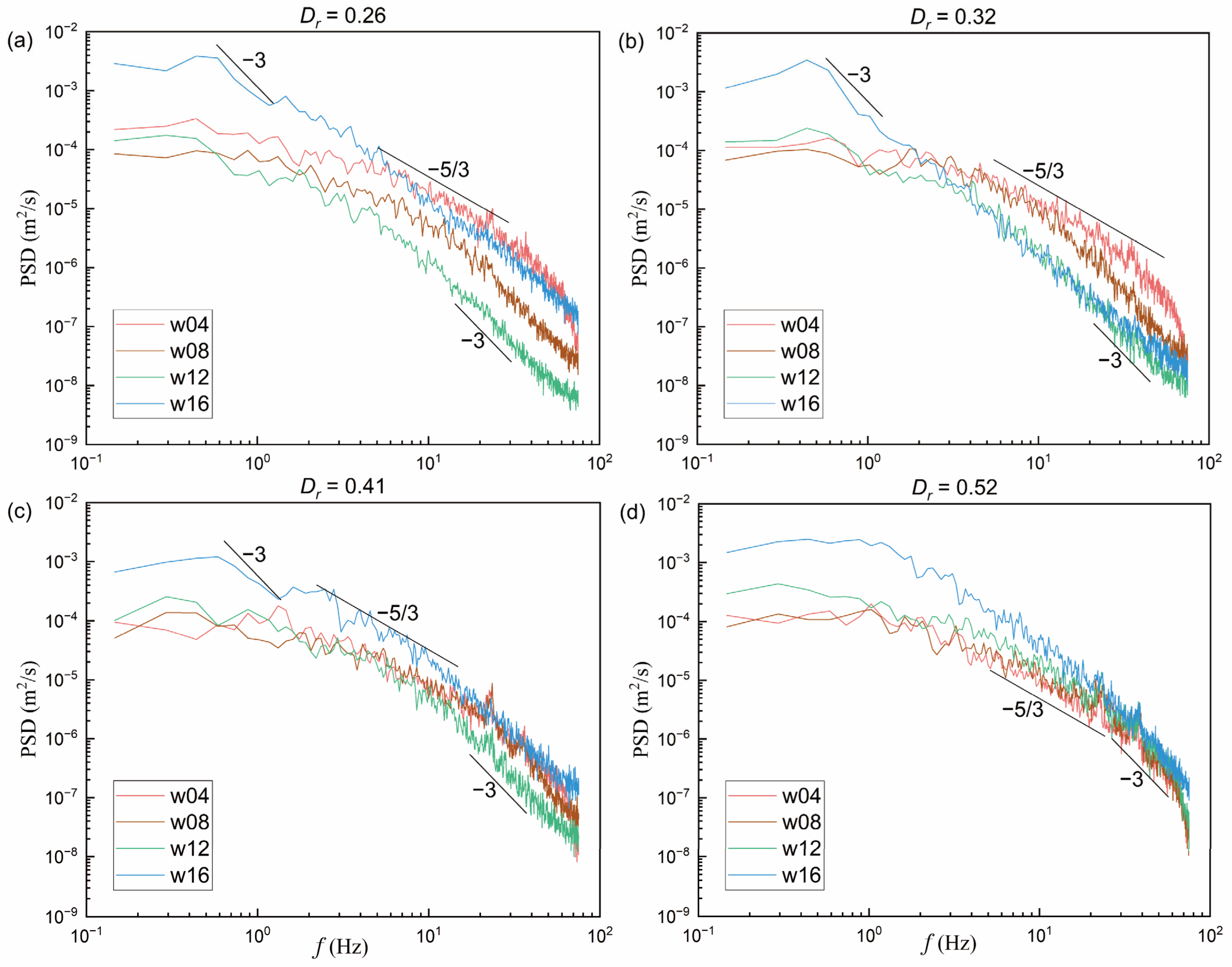
Power spectral density (PSD) and normalized temporal autocorrelation analyses of the spanwise velocity fluctuations, $v^{\prime }$, were conducted at four representative locations: the center of the main channel, w04 (y = 20 cm); the main-channel/floodplain interface, w08 (y = 34 cm); the center of the non-vegetated floodplain, w12 (y = 48 cm); and the outer edge of the vegetated region near the floodplain sidewall, w16 (y = 67 cm). Following Uijttewaal and Booij [36] and Truong and Uijttewaal [18], measurements obtained at approximately mid-depth were selected for these analyses.

After quality control, the isolated missing samples were linearly interpolated onto the original uniform 200 Hz time grid. The reconstructed records were then processed using a fourth-order Butterworth low-pass filter with a design cutoff frequency of 70 Hz. The filter was applied in the forward and reverse directions using the MATLAB filtfilt function, thereby producing a zero-phase response and minimizing endpoint transients. The filtered records were subsequently resampled at 150 Hz using linear interpolation.

The PSD was estimated using Welch’s method. Each record was divided into segments of 1024 samples, corresponding to 6.83 s at the resampled frequency, and a Hamming window was applied to each segment. Adjacent segments overlapped by 32 samples, corresponding to 0.213 s or 3.125% of the segment length. A 1024-point fast Fourier transform was used, resulting in a frequency-bin spacing of approximately 0.146 Hz and a one-sided frequency range of 0–75 Hz.

Following the framework discussed by Proust, Fernandes, Leal, Rivière and Peltier [12], pure two-dimensional (2D) turbulence and quasi-two-dimensional turbulence were considered as idealized regimes for interpreting the spectra. In classical pure 2D turbulence, the absence of vortex stretching permits a dual-cascade process, with a −5/3 wavenumber-spectrum scaling in the inverse energy-cascade range and a −3 scaling in the forward enstrophy-cascade range. Quasi-2D turbulence may retain limited vertical motion and weak vortex stretching. Following Uijttewaal and Booij [36], a distinct spectral peak followed on its high-frequency side by an approximately −3 decay was regarded as evidence consistent with large-scale motions possessing quasi-two-dimensional characteristics [10,12,36,37,38]. However, the theoretical dual-cascade scaling laws are defined for wavenumber spectra. Therefore, analogous slopes in the present fixed-point frequency spectra were used as diagnostic reference scaling rather than, by themselves, definitive evidence of turbulence dimensionality or the direction of spectral energy transfer. In the present analysis, a localized spectral peak, an approximately −3 spectral decay, and a slowly decaying or oscillatory temporal autocorrelation were considered jointly when identifying long-lived, quasi-2D coherent motions.

The normalized temporal autocorrelation of $v^{\prime }$ was used to examine the persistence of velocity fluctuations and identify long-time-correlated motions associated with the MCFP and NVV shear layers. Following previous studies [12,19,36], the autocorrelation function was calculated as:

$$R_{vv}\left(\tau \right)={\displaystyle \frac{\overline{v^{\prime }\left(t_0\right)·v^{\prime }\left(t_0+\tau \right)}}{\sqrt{\overline{\left({v^{\prime }}^2\left(t_0\right)·{v^{\prime }}^2\left(t_0+\tau \right)\right)}}}}$$

(19)

where $t_0$ denotes an arbitrary reference time; $\tau$ represents the time lag between two samples $v^{\prime }\left(t_0\right)$ and $v^{\prime }\left(t_0+\tau \right)$ from the same velocity-fluctuation record measured at a single location.

A rapid initial decrease in $R_{vv}\left(\tau \right)$ was interpreted as the decorrelation of relatively small-scale fluctuations, whereas a slowly decaying or oscillatory component was interpreted as evidence consistent with longer-lived coherent motions. The first distinct shoulder or change in decay rate following the rapid initial decrease was used to define an approximate transition lag, ${\tau }_c$. Under the assumption that the rapidly decorrelating component had become negligible by ${\tau }_c$, while the large-scale component remained correlated, $R_{vv}\left({\tau }_c\right)$ was used as an approximate indicator of the fraction of spanwise velocity variance associated with long-time-correlated motions.

It should be noted that ChatGPT was used as a coding assistant during the development, debugging, and refinement of the MATLAB and Python scripts used to implement the data-processing procedures described above, including data organization, interpolation and resampling, power spectral density and temporal autocorrelation analyses, calculation of depth-averaged quantities and transverse momentum-exchange terms, and visualization of the processed results. The tool was used primarily to provide suggestions on code structure, correct syntax, diagnose programming errors, and refine the implementation of the specified analytical procedures. All AI-assisted scripts and computational outputs were independently reviewed, tested, and validated by the authors against the original measurements and expected numerical behavior before being used to produce the results reported in this study.

4. Results and Discussion

4.1. Lateral Distributions of Streamwise Velocity

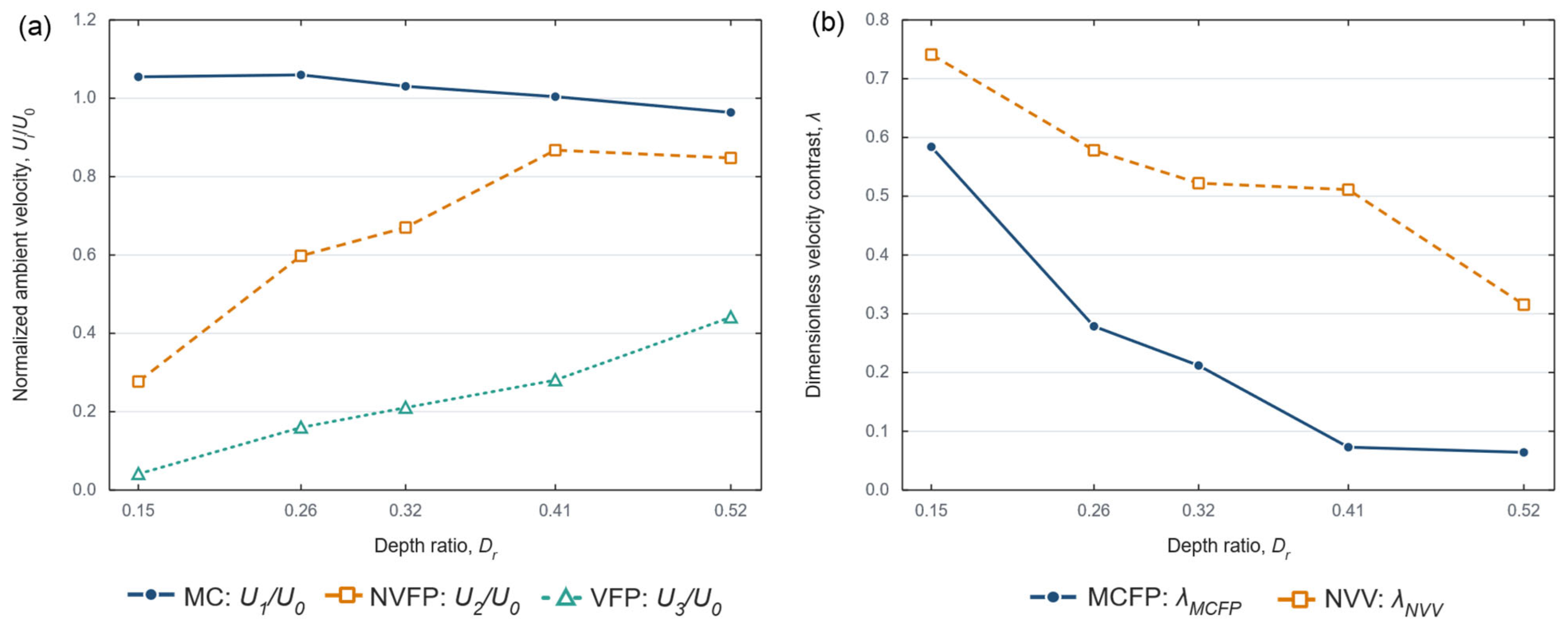
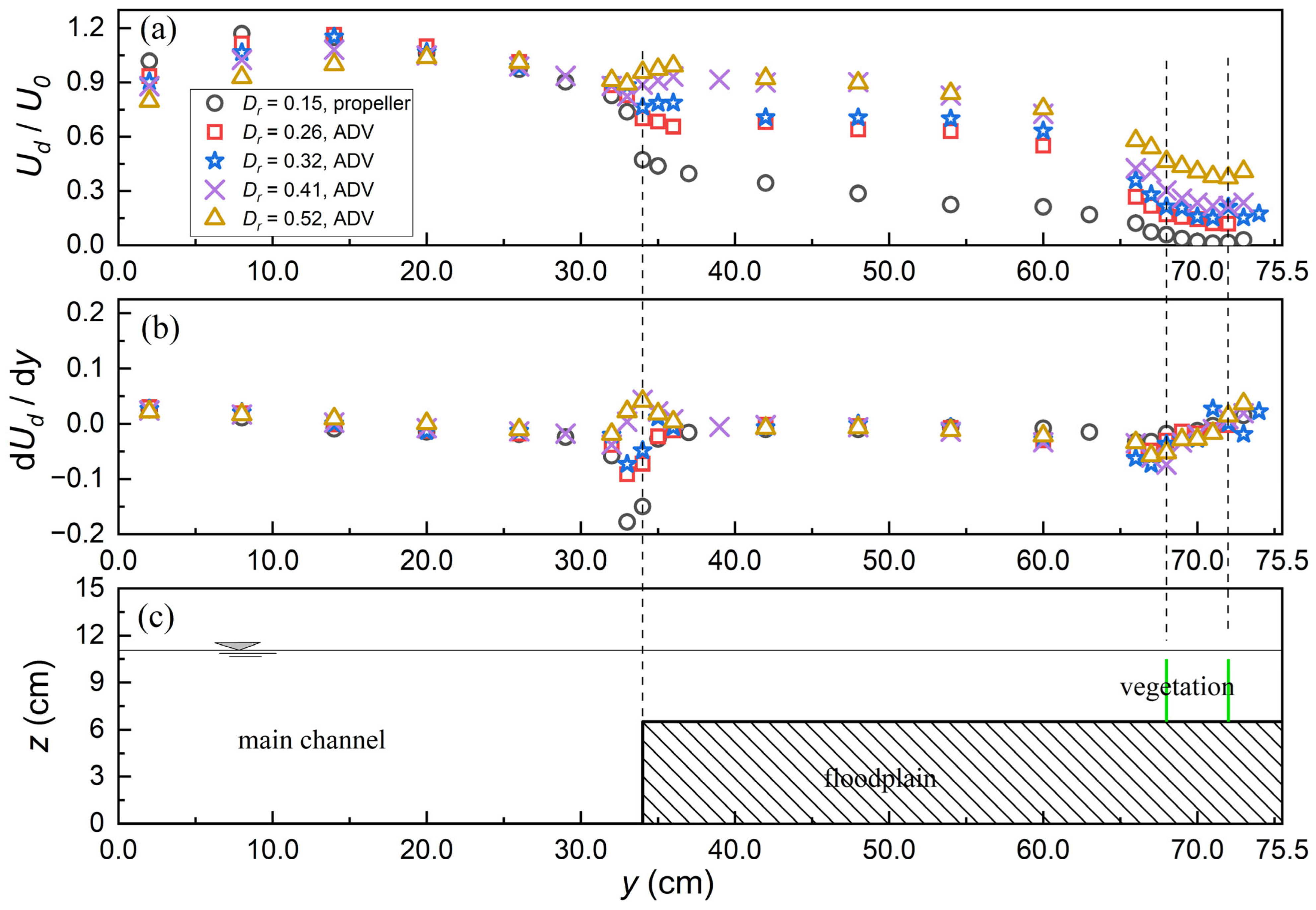
Figure 2 presents the lateral distributions of the normalized depth-averaged streamwise $U_d/U_0$ and the corresponding lateral velocity gradient, $d{U}_d/dy$, across the compound-channel cross-section. For all five investigated depth ratios, the highest velocities occurred in the main channel (MC), intermediate velocities occurred in the non-vegetated floodplain (NVFP), and the lowest velocities occurred in the vegetated floodplain (VFP). This distribution resulted primarily from the elevated floodplain bed and the additional drag exerted by vegetation in the VFP. As $D_r$ increased from 0.15 to 0.52, $U_1/U_0$ decreased from 1.055 to 0.964, whereas $U_2/U_0$ increased from 0.277 to 0.848 and $U_3/U_0$ increased from 0.041 to 0.441 (

Table 3. Ambient velocities and quantitative characteristics of the two lateral shear layers under different depth ratios.

${\mathit{D}}_{\mathit{r}}$	$\frac{{\mathit{U}}_1}{{\mathit{U}}_0}$	$\frac{{\mathit{U}}_2}{{\mathit{U}}_0}$	$\frac{{\mathit{U}}_3}{{\mathit{U}}_0}$	${\mathit{\lambda }}_{\mathit{M}\mathit{C}\mathit{F}\mathit{P}}$	${\mathit{\lambda }}_{\mathit{N}\mathit{V}\mathit{V}}$	${\mathit{t}}_{\mathit{M}\mathit{C}\mathit{F}\mathit{P}}$ (cm)	${\mathit{t}}_{\mathit{N}\mathit{V}\mathit{V}}$ (cm)	${\mathit{\theta }}_{\mathit{M}\mathit{C}\mathit{F}\mathit{P}}$ (cm)	${\mathit{\theta }}_{\mathit{N}\mathit{V}\mathit{V}}$ (cm)
0.15	1.06	0.28	0.04	0.58	0.74	23.48	18.51	2.81	3.30
0.26	1.06	0.60	0.16	0.28	0.58	27.92	9.49	3.71	1.59
0.32	1.03	0.67	0.21	0.21	0.52	22.80	8.34	3.50	1.52
0.41	1.00	0.87	0.28	0.07	0.51	11.88	14.03	1.90	2.42
0.52	0.96	0.85	0.44	0.06	0.32	16.97	11.60	2.13	2.21

Note: $U_1$, $U_2$ and $U_3$ denote the representative ambient depth-averaged streamwise velocities in the MC, NVFP, and VFP, respectively, as defined in Section 3.1. Here, $t$ and $\theta$ denote the nominal and momentum thicknesses of the corresponding shear layers, respectively.

). These variations indicate a progressive redistribution of normalized streamwise velocity from the MC toward the floodplain as the relative floodplain depth increased.

The lateral velocity profiles contained two relatively low-gradient ambient regions, located in the MC and NVFP, consistent with the equilibrium regions reported in previous compound-channel studies [19,34,39]. Two pronounced lateral shear layers were also identified: the main-channel/floodplain (MCFP) shear layer between the MC and NVFP and the non-vegetated/vegetated (NVV) shear layer between the faster NVFP and the slower VFP. The coexistence of these two shear layers agrees with the observations of Zhang and Hu [19]. However, the two layers responded differently to variations in $D_r$.

The absolute velocity difference across the MCFP interface decreased from 39.55 cm/s at $D_r=0.15$ to 6.43 cm/s at $D_r=0.52$. Correspondingly, ${\lambda }_{MCFP}$ decreased from 0.58 to 0.06, representing an approximately 89% reduction. In contrast, the absolute velocity difference across the NVV interface increased from 11.99 cm/s at $D_r=0.15$ to a maximum of 27.41 cm/s at $D_r=0.41$, before decreasing to 22.50 cm/s at $D_r=0.52$. Nevertheless, ${\lambda }_{NVV}$ decreased from 0.74 to 0.32 because the ambient velocities on both sides of the NVV interface increased with $D_r$.

In all five cases, ${\lambda }_{NVV}$ exceeded ${\lambda }_{MCFP}$, demonstrating that the vegetation boundary maintained a greater relative velocity contrast than the topographic MCFP interface. Moreover, from $D_r=0.32$ onward, the absolute velocity difference across the NVV interface also exceeded that across the MCFP interface. These results indicate that increasing $D_r$ strongly weakened the conventional MCFP shear layer, whereas vegetation drag maintained a substantial velocity contrast between the faster NVFP and the slower VFP. Consequently, the relative importance of the NVV shear layer increased under the intermediate- and deep-flow conditions. The corresponding variations in the normalized ambient velocities and dimensionless shear parameters are summarized in Figure 3.

The nominal and momentum thicknesses did not vary monotonically with $D_r$. For example, $t_{MCFP}$ initially increased from 23.48 cm at $D_r=0.15$ to 27.92 cm at $D_r=0.26$, subsequently decreased to 11.88 cm at $D_r=0.41$, and then increased to 16.97 cm at $D_r=0.52$. Similar non-monotonic variations were observed in the NVV shear-layer thicknesses. Therefore, the decrease in dimensionless velocity contrast did not necessarily correspond to a proportional reduction in shear-layer width. This distinction suggests that $D_r$ affected the intensity and spatial extent of the two shear layers through related but different processes.

de Oliveira, Janzen, Folke, Wittmann, Huber, Franca and Gualtieri [14] similarly reported that floodplain vegetation increased lateral shear through the additional drag imposed on the floodplain flow and that the dimensionless shear decreased with increasing relative water depth. The reductions in both ${\lambda }_{MCFP}$ and ${\lambda }_{NVV}$ observed in the present study are consistent with this depth-dependent tendency. However, their vegetation occupied the full floodplain width and primarily strengthened the MCFP mixing layer, whereas the present partial-width vegetation introduced an additional NVV shear layer within the floodplain. Furthermore, their study compared vegetated conditions with corresponding bare cases and examined longitudinal flow adjustment, whereas the present comparison concerns different $D_r$ values under a fixed partial-vegetation arrangement. Therefore, their vegetation-induced increase in MC velocity relative to bare conditions does not conflict with the present decrease in normalized MC velocity as $D_r$ increased.

The shape of the lateral velocity profile within the MCFP region also exhibited a clear dependence on $D_r$. The profiles at $D_r$ = 0.15, 0.26, and 0.32 were monotonic, consistent with the shallow-flow regime reported in previous studies [12]. At $D_r=0.41$, a velocity dip developed near the MCFP interface, resulting in a non-monotonic profile characteristic of the intermediate-flow regime [12,19]. A similar velocity dip remained evident at $D_r=0.52$, although this case falls within the nominal deep-flow range according to the conventional threshold (i.e., $D_r>0.5$ as described in Section 1). Therefore, the smoother transition-zone profile previously reported for deep non-vegetated compound-channel flows [9] was not observed in the present partially vegetated configuration.

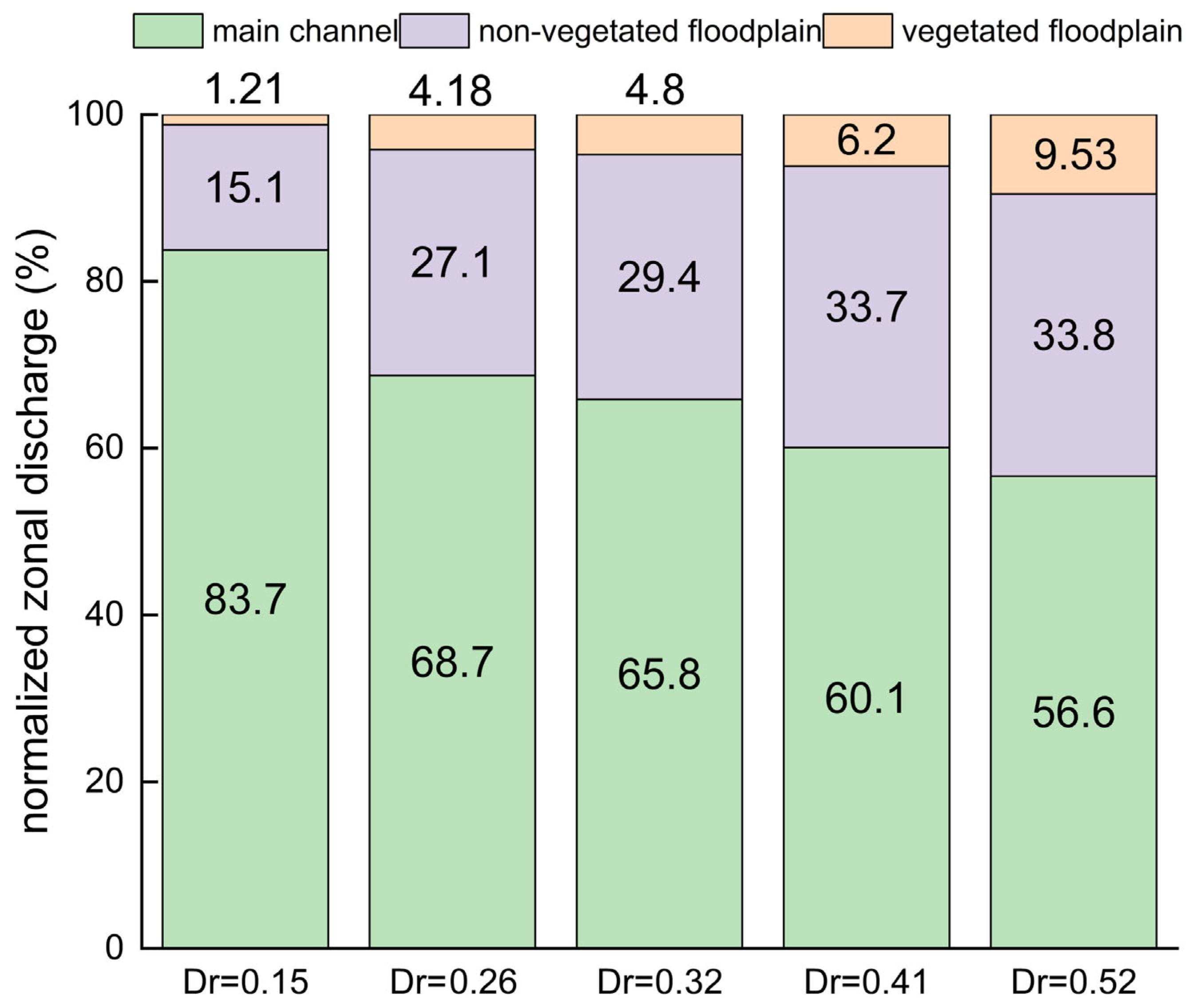
The velocity redistribution identified in Figure 2 is further quantified by the normalized zonal discharge shown in Figure 4. Figure 4 presents the proportions of the total discharge conveyed by the MC, NVFP, and VFP under different depth ratios. The three zones correspond to measurement positions w01–w07, w08–w14, and w15–w23, respectively. This subdivision follows the cross-sectional geometry and vegetation arrangement.

As shown in Figure 4, when $D_r$ increased from 0.15 to 0.52, the proportion of the total discharge conveyed by the MC decreased from 83.7% to 56.6%. In contrast, the NVFP contribution increased from 15.1% to 33.8%, while the VFP contribution increased from 1.21% to 9.53%. The combined floodplain discharge fraction therefore increased from 16.31% to 43.33%. This quantitatively confirms that increasing the relative floodplain depth enhanced the floodplain contribution to total conveyance, despite the velocity reduction caused by vegetation within the VFP.

Overall, increasing $D_r$ produced two related changes: it redistributed streamwise velocity and discharge from the MC toward the floodplain, and it modified the velocity contrasts across the MCFP and NVV interfaces differently. The quantified ambient velocities, velocity differences, and dimensionless shear parameters in Table 3 and Figure 3 provide the basis for interpreting the Reynolds-stress distributions and transverse momentum-exchange mechanisms discussed in Section 4.3.

4.2. Vertical Distribution of Streamwise Velocity

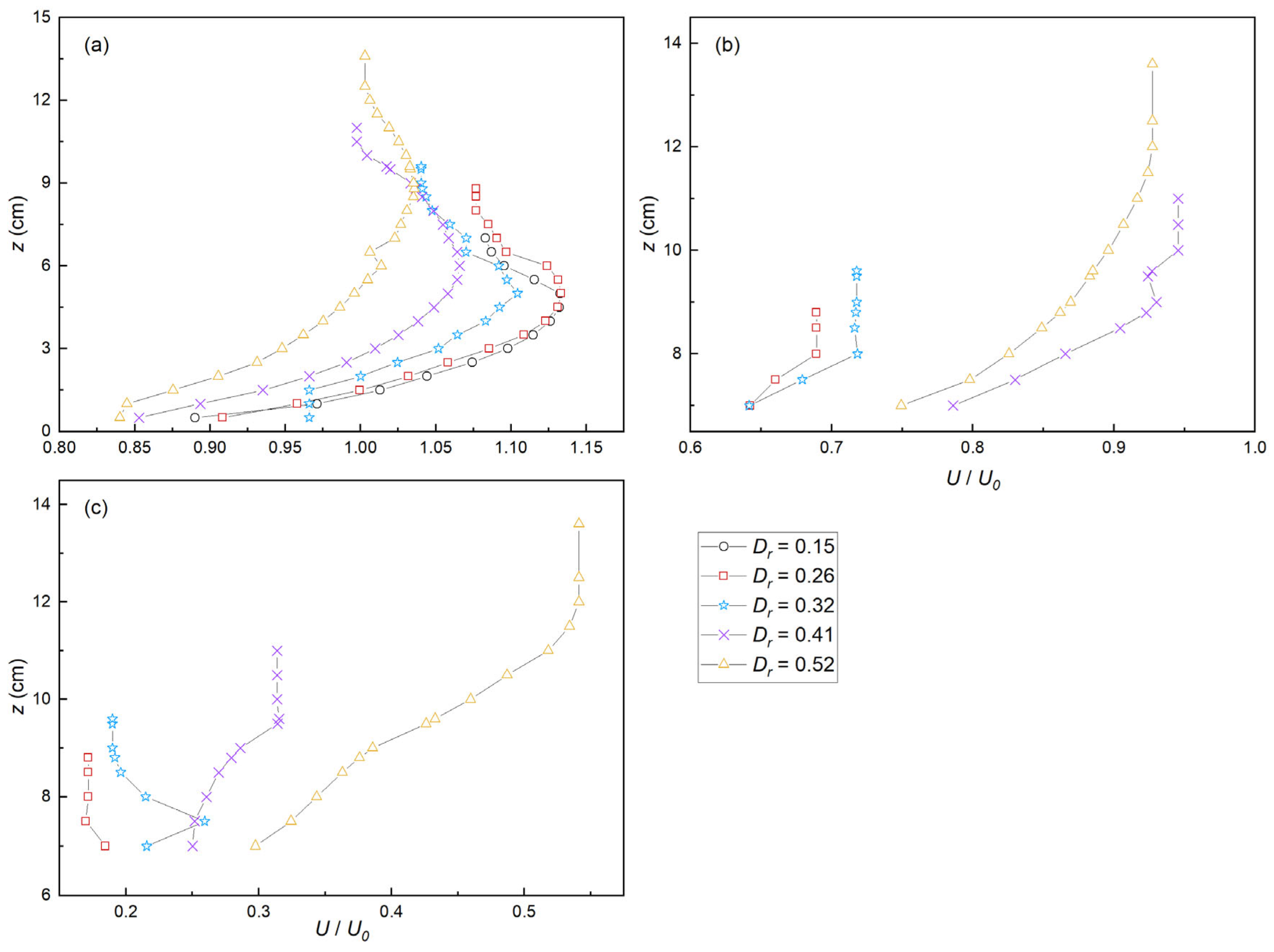
To facilitate direct comparison among the investigated depth ratios, Figure 5 presents the zonal-averaged vertical profiles of streamwise velocity in the MC, NVFP, and VFP. The streamwise velocity $U$ was normalized by the corresponding channel-averaged velocity, $U_0$, whereas the physical vertical coordinate z was retained. Because the lateral measurement positions were unevenly spaced, representative-width weighting was applied when calculating the zonal averages. Interpolation was restricted to the vertical range supported by the measurements, and no vertical extrapolation was performed. Due to the limited floodplain measurement points for $D_r=0.15$, it was excluded in Figure 5b,c.

The MC profiles exhibited an increase in $U/U_0$ from the near-bed region to a subsurface maximum, followed by a decrease toward the uppermost measured level (Figure 5a). The maximum $U$ was approximately 1.133 at z = 5.0 cm for $D_r=0.15$ and 0.26, 1.104 at z = 5.0 cm for $D_r=0.32$, 1.066 at z = 6.0 cm for $D_r=0.41$, and 1.036 at z = 8.8 cm for $D_r=0.52$. Thus, as $D_r$ increased, the absolute elevation of the maximum velocity moved upward, whereas its magnitude relative to $U_0$ generally decreased.

At the uppermost supported measurement level, $U/U_0$ was approximately 3.2–6.4% lower than the corresponding subsurface maximum. A dip-like structure therefore remained visible in the zonal MC profiles for all cases, although its magnitude varied non-monotonically with $D_r$ and was weakest for $D_r=0.52$. Subsurface velocity maxima have previously been associated with secondary-flow-induced momentum redistribution in compound channels [40,41,42,43,44]. However, because the present measurements do not directly resolve closed cross-sectional circulation cells, the observed velocity dip is interpreted as a secondary-flow-related signature rather than as direct evidence of a particular macrovortex orientation.

The floodplain profiles responded differently to changes in $D_r$ (Figure 5b,c). At z = 7.5 cm, $U/U_0$ in the NVFP increased from 0.358 at $D_r=0.15$ to 0.660, 0.679, 0.830, and 0.798 at $D_r=0.26$, 0.32, 0.41, and 0.52, respectively. Although the normalized values did not vary strictly monotonically, the deeper cases exhibited substantially higher NVFP velocities than the shallowest case. This indicates an overall enhancement of streamwise flow within the non-vegetated floodplain as the relative floodplain depth increased.

The VFP velocities remained markedly lower than the NVFP velocities because of vegetation drag. At z = 7.5 cm, $U/U_0$ in the VFP increased overall from 0.049 at $D_r=0.15$ to 0.170, 0.259, 0.252, and 0.324 for the successively deeper cases. The normalized velocity difference between the NVFP and VFP at this elevation ranged from approximately 0.309 to 0.578. Thus, although increasing $D_r$ enhanced the velocities in both floodplain regions, a pronounced lateral velocity contrast persisted across the NVV interface. This persistent contrast provides the mean-flow basis for the vegetation-induced lateral shear layer and the Reynolds-stress distributions examined in Section 4.3.

For the deeper cases, particularly $D_r=0.52$, the VFP velocity increased substantially above the vegetation layer. The corresponding change in profile shape is consistent with the canopy-top mixing-layer behavior previously observed in submerged vegetation flows [32,45,46,47]. In contrast, under shallower conditions, the limited flow depth and the larger relative influence of vegetation drag restricted the development of flow above the vegetation. Increasing $D_r$ therefore affects the floodplain profile through both increased flow depth and changing vegetation submergence.

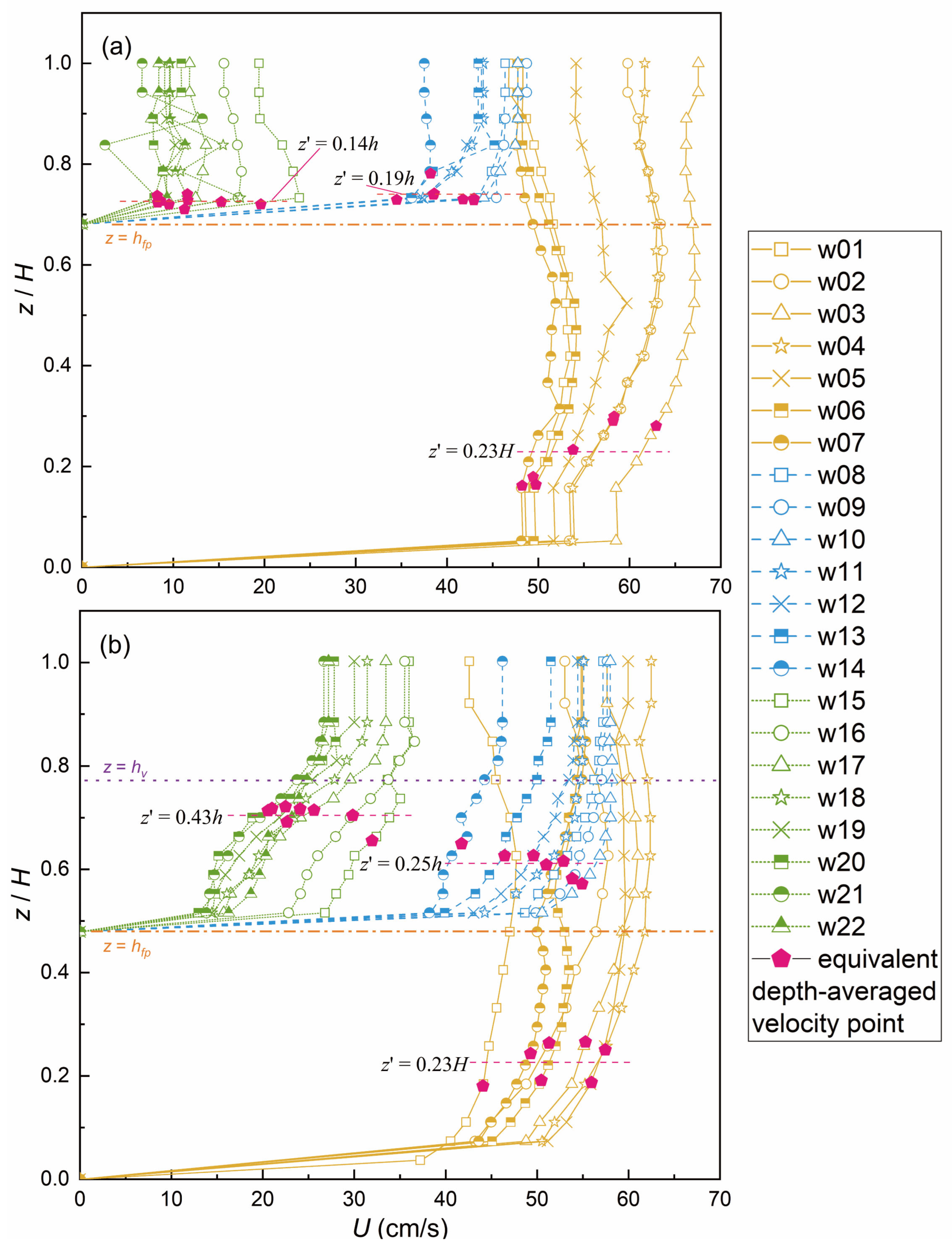
The zonal averages in Figure 5 reveal the overall depth-ratio dependence, whereas the profiles at individual lateral measurement positions in Figure 6 illustrate the corresponding spatial variability. For $D_r=0.32$, subsurface velocity maxima occurred at several MC and VFP positions, while the NVFP profiles more closely resembled conventional boundary-layer profiles controlled primarily by bed friction [47,48]. For $D_r=052$, some MC profiles became smoother toward the water surface, although the zonal MC average retained a modest subsurface maximum. Within the VFP, the individual profiles exhibited a hyperbolic-tangent-like shape with an inflection region close to or above the vegetation top, consistent with the development of a vegetation-induced mixing layer [32,45,46,47].

Figure 5 and Figure 6 therefore provide complementary information. Figure 5 demonstrates how the average vertical flow structure in each zone varies with $D_r$, whereas Figure 6 shows that substantial lateral variability remains within each zone. The regionally averaged profiles should consequently not be interpreted as replacing the individual measurements, but as providing a clearer comparison of the overall depth-ratio effect requested by the reviewer.

In addition to characterizing the vertical profile shapes, the individual profiles in Figure 6 were used to identify the elevation at which the local streamwise velocity equals the corresponding depth-averaged velocity, $U_d$. Previous studies have frequently used the mid-depth velocity as an approximation for $U_d$ [18,34,49]. However, the subsurface maxima observed in the present compound-channel profiles indicate that the mid-depth approximation may not provide the most representative estimate.

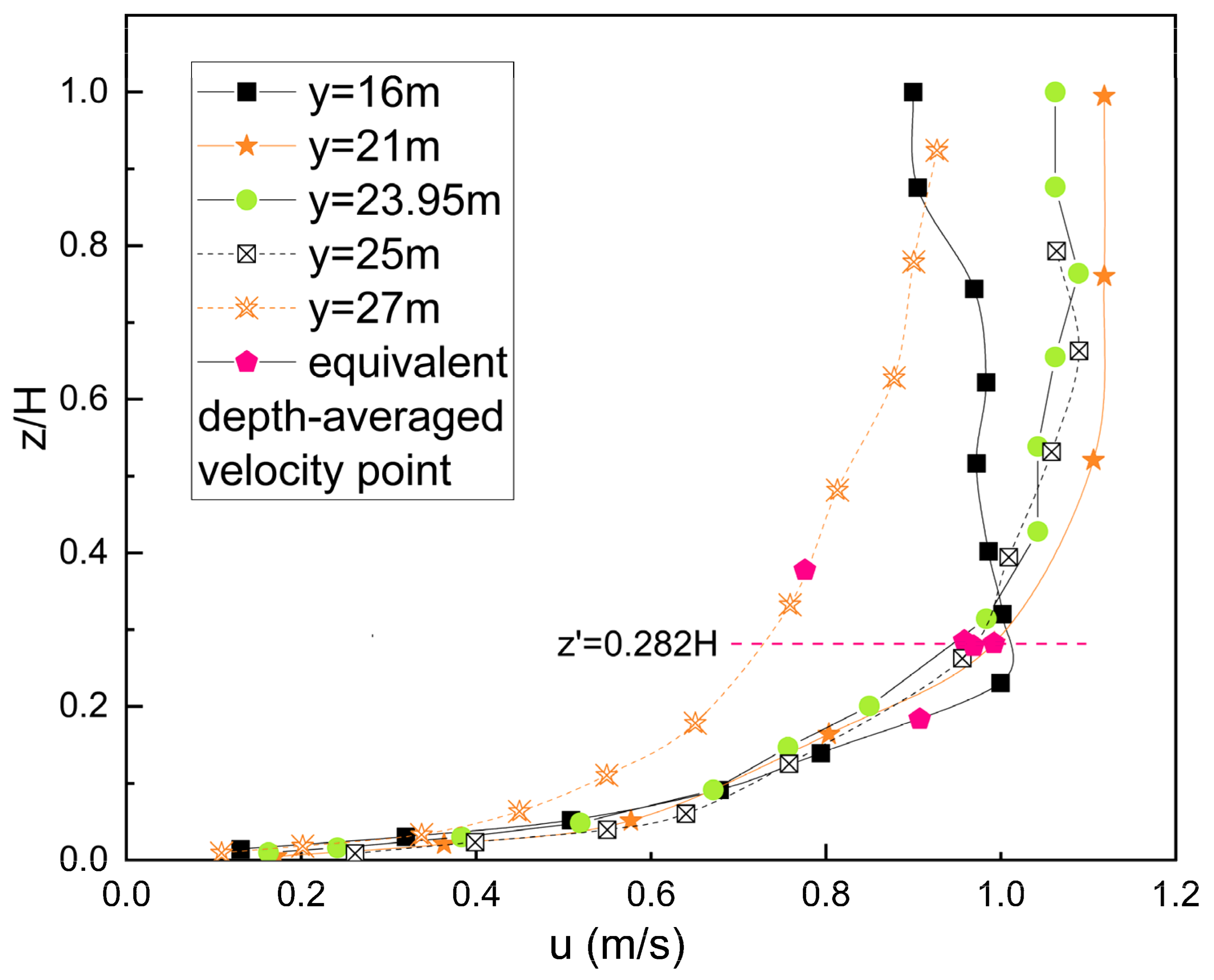
As indicated by the filled symbols and horizontal dashed lines in Figure 6, the equivalent elevation in the MC was generally close to z = 0.23H. This result is broadly consistent with the field measurements of Carling et al. [50]. Figure 7 was redrawn by the authors using the data reported Carling, Cao, Holland, Ervine and Babaeyan-Koopaei [50] and shows that the streamwise velocity measured at approximately z = 0.28H provided a reasonable estimate of the local depth-averaged velocity in the natural compound channel examined in that study. Accordingly, the practical approximation $U_d=U at 0.25H$ was evaluated for the MC measurement positions under $D_r=0.26$, 0.32, 0.41, and 0.52.

The results are summarized in

Table 4. The error analysis of the modeled results of the 0.25H method.

Point	y Position (cm)	${\mathit{D}}_{\mathit{r}}$ = 0.26			${\mathit{D}}_{\mathit{r}}$ = 0.32
		${\mathit{U}}_{\mathit{d}}$ (cm/s)	Modeled ${\mathit{U}}_{\mathit{d}}$ (cm/s)	Error (%)	${\mathit{U}}_{\mathit{d}}$ (cm/s)	Modeled ${\mathit{U}}_{\mathit{d}}$ (cm/s)	Error (%)
w01	2	46.92	49.14	4.74	49.44	51.43	4.03
w02	8	55.92	56.14	0.39	58.20	57.18	−1.74
w03	14	58.44	59.18	1.28	62.94	62.31	−1.00
w04	20	55.17	54.45	−1.31	58.31	57.13	−2.02
w05	26	50.83	51.37	1.05	53.81	54.35	1.00
w06	32	44.32	46.78	5.54	49.74	52.22	4.99
w07	33	41.55	43.30	4.22	48.23	49.99	3.67
Point	y  position (cm)	${\mathit{D}}_{\mathit{r}}$ = 0.41			${\mathit{D}}_{\mathit{r}}$ = 0.52
		${\mathit{U}}_{\mathit{d}}$ (cm/s)	Modeled ${\mathit{U}}_{\mathit{d}}$ (cm/s)	Error (%)	${\mathit{U}}_{\mathit{d}}$ (cm/s)	Modeled ${\mathit{U}}_{\mathit{d}}$ (cm/s)	Error (%)
w01	2	41.04	43.09	4.99	44.07	44.74	1.51
w02	8	47.81	46.43	−2.89	51.32	51.14	−0.36
w03	14	50.45	49.59	−1.71	55.29	55.13	−0.30
w04	20	48.97	49.01	0.09	57.43	57.63	0.34
w05	26	46.11	47.03	2.00	55.95	57.41	2.61
w06	32	41.11	41.06	−0.13	50.46	52.04	3.13
w07	33	38.45	36.40	−5.33	49.29	49.60	0.61

. The mean absolute errors were 2.65%, 2.64%, 2.45%, and 1.27% for $D_r=0.26$, 0.32, 0.41, and 0.52, respectively. Across all the evaluated MC profiles, the overall mean absolute error was 2.25%, among which over 93% of the estimates had absolute errors not exceeding 5%, and the maximum absolute error was 5.54%. The $D_r=0.15$ case was excluded because the number of available vertical measurements was insufficient for a reliable evaluation.

The representative elevation of approximately 0.25H is lower than the value of approximately 0.37H expected from an ideal logarithmic velocity distribution. This downward displacement may reflect the combined influences of the velocity-dip phenomenon, secondary-flow-related momentum redistribution, and lateral momentum exchange. Because the cross-sectional circulation responsible for this displacement was not measured directly, this explanation remains a physical interpretation rather than a confirmed causal relationship.

The 0.25H approximation is supported here for the examined MC profiles but should not be applied universally to the floodplain. The equivalent elevations within the NVFP and VFP showed greater variability because their profile shapes were additionally affected by floodplain-bed resistance, vegetation drag, and vegetation submergence. Further experiments covering different channel geometries, vegetation arrangements, and relative flow depths are required before a universal representative elevation can be established.

Overall, increasing $D_r$ reduced the normalized MC velocity maximum while enhancing the velocities in the NVFP and VFP. Nevertheless, the velocity difference between the non-vegetated and vegetated floodplain regions remained substantial, indicating that the vegetation-induced NVV shear layer persisted throughout the investigated range. These depth-ratio-dependent changes in vertical velocity structure and lateral velocity contrast provide the basis for interpreting the transverse momentum exchange and turbulent structures presented in Section 4.3 and Section 4.4.

4.3. Transverse Momentum Exchange

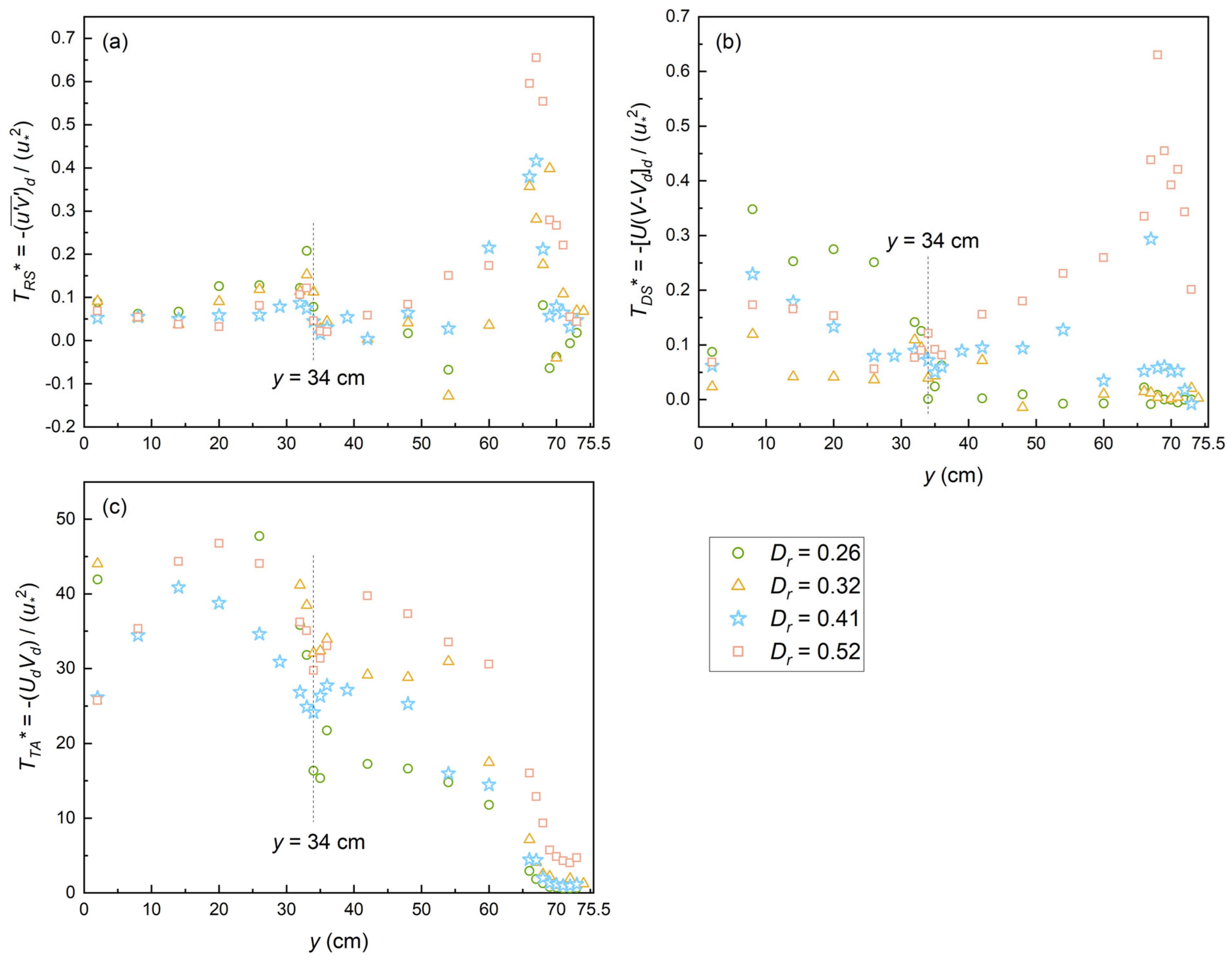
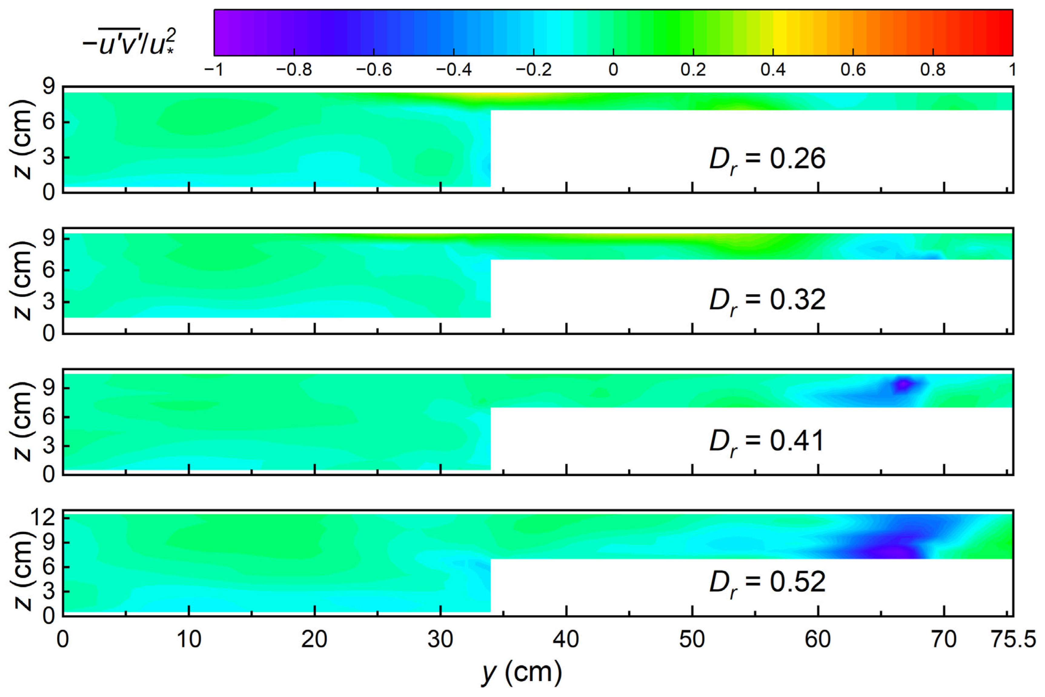
This section examines the depth-averaged transverse exchange of streamwise momentum for the four ADV-measured cases, $D_r=0.26$, 0.32, 0.41, and 0.52. As defined in Section 3.2, Figure 8 presents the lateral distributions of the normalized Reynolds-stress contribution, $T_{RS}^{\ast }$, mean transverse-advection contribution $T_{TA}^{\ast }$, and secondary-current-related dispersive contribution $T_{DS}^{\ast }$. Under the sign convention adopted in Equation (10), a negative value of any contribution represents streamwise-momentum transport in the positive y-direction, i.e., from the MC toward the FP, whereas a positive value represents transport in the negative y-direction, i.e., from the FP toward the MC. Figure 9 separately presents the cross-sectional distribution of the local normalized Reynolds shear stress, $R_{uv}^{\ast }\left(y,z\right)=-\overline{u^{\prime }{v}^{\prime }}/{u_{\ast }}^2$.

Table 5. Case-wise summary of transverse momentum exchange.

${\mathit{D}}_{\mathit{r}}$	$\mathit{m}\mathit{a}\mathit{x}\left|{\mathit{T}}_{\mathit{T}\mathit{A}}^{\mathit{*}}\right|$	$\mathit{m}\mathit{a}\mathit{x}\left|{\mathit{T}}_{\mathit{R}\mathit{S}}^{\mathit{*}}\right|$	$\mathit{m}\mathit{a}\mathit{x}\left|{\mathit{T}}_{\mathit{D}\mathit{S}}^{\mathit{*}}\right|$	$\frac{\mathit{m}\mathit{a}\mathit{x}\left|{\mathit{T}}_{\mathit{T}\mathit{A}}^{\mathit{*}}\right|}{\mathit{m}\mathit{a}\mathit{x}\left|{\mathit{T}}_{\mathit{R}\mathit{S}}^{\mathit{*}}\right|}$	$\frac{\mathit{m}\mathit{a}\mathit{x}\left|{\mathit{T}}_{\mathit{T}\mathit{A}}^{\mathit{*}}\right|}{\mathit{m}\mathit{a}\mathit{x}\left|{\mathit{T}}_{\mathit{D}\mathit{S}}^{\mathit{*}}\right|}$	Correlation Coefficient Between ${\left({\mathit{T}}_{\mathit{y}\mathit{x}}\right)}_{\mathit{d}}^{\mathit{*}}$ and ${\mathit{T}}_{\mathit{T}\mathit{A}}^{\mathit{*}}$	Maximum Relative Difference (%)
0.26	73.958	0.208	0.348	356.339	212.633	1.000	0.6
0.32	66.454	0.398	0.119	166.883	556.662	1.000	0.7
0.41	40.843	0.416	0.294	98.151	139.150	1.000	1.7
0.52	46.756	0.655	0.630	71.379	74.217	1.000	2.5

summarizes the case-wise maximum absolute magnitudes of the three transverse momentum-exchange contributions, their magnitude ratios, and the agreement between the total momentum exchange and the mean transverse-advection contribution. Across all four analyzed cases, the mean transverse-advection contribution was the dominant mechanism of transverse momentum exchange. The maximum absolute magnitude of $T_{TA}^{\ast }$ ranges from 40.84 to 73.96, compared with 0.208–0.655 for $T_{RS}^{\ast }$ and 0.119–0.630 for $T_{DS}^{\ast }$. Based on the case-wise maximum-magnitude comparison, max $\left|T_{TA}^{\ast }\right|$ exceeds max $\left|T_{RS}^{\ast }\right|$ by factors of 71.4–356.3 and exceeds max $\left|T_{DS}^{\ast }\right|$ by factors of 74.2–556.7. These ratios quantify differences in the characteristic peak magnitudes of the three mechanisms rather than their fractional contributions at a common lateral position. Thus, the mean transverse-advection contribution was approximately two orders of magnitude greater than the Reynolds-stress and dispersive-stress contributions across the measured cases. The total normalized transverse momentum flux, ${\left(T_{yx}\right)}_d^{\ast }$, therefore closely follows the spatial distribution of $T_{TA}^{\ast }$. The case-wise correlation between ${\left(T_{yx}\right)}_d^{\ast }$ and $T_{TA}^{\ast }$ ranged from 0.99986 to 0.99999, while the maximum difference between them was only 0.6–2.5% of the case-wise maximum total flux. These results demonstrate that for the partially vegetated floodplain configuration in this study, mean transverse advection controlled both the magnitude and the lateral variation in the total transverse momentum exchange at the measured cross-section.

A consistent depth-averaged mean transverse flow from the FP toward the MC was observed across the four ADV-measured cases. This direction agrees with the vegetation-induced flow readjustment reported by de Oliveira, Janzen, Folke, Wittmann, Huber, Franca and Gualtieri [14], in which increased floodplain roughness diverted flow toward the main channel. However, the vegetation configurations differ: their forest occupied the full floodplain width and introduced a longitudinal roughness transition, whereas the present vegetation occupies only part of the floodplain width and introduces an additional NVV shear layer.

The results indicate that transverse flow dominates lateral momentum exchange, with a magnitude roughly two orders of magnitude higher than that of the Reynolds stress and secondary flow terms. This finding highlights transverse flow as the primary driver of lateral momentum transfer in the system.

For all depth ratios, the Reynolds stress term remains relatively constant and near zero within the main channel (Figure 8a), indicating that turbulent mixing in this region can be considered negligible. Within the MCFP mixing layer, cases $D_r=$ 0.26 and 0.32 exhibit a peak at the interface, whereas $D_r=$ 0.41 and 0.52 show smoother profiles. This observation aligns with the findings of Ackers [11] and Ikeda and McEwan [51], who reported the strongest MCFP interaction at $D_r\approx 0.2~0.3$. On the floodplain, Reynolds stress in the NVV shear layer increases with the depth ratio, which is expected because submerged vegetation creates an additional mixing layer at the canopy, enhancing turbulent mixing.

Across all depth ratios, the highest Reynolds stress consistently appears at the interface between non-vegetated and vegetated zones. Figure 9 corroborates this by illustrating the cross-sectional distribution of Reynolds stress. Notably, the location of maximum Reynolds stress here differs from previous studies on fully vegetated or non-vegetated compound channels [12,18], where the peak typically lies within the MCFP mixing layer. This discrepancy likely arises from the limited interaction between the NVV mixing layer and the MCFP mixing layer, attributed to the relatively narrow vegetated region and low plant density [19].

Figure 9 presents the cross-sectional distributions of normalized Reynolds stress for varying depth ratios. Both the magnitude and spatial extent of the Reynolds shear stress generally increased with water depth. The elevated Reynolds shear stress near the NVV interface, consistent with Figure 8a, is associated with the additional lateral shear layer generated at the boundary between the non-vegetated and vegetated floodplain regions [46,47].

Within the MCFP mixing layer, the secondary flow remains relatively uniform across different water depths. However, in the main channel and on the floodplain, the behavior of the secondary flow term varies significantly with depth ratio. For the intermediate flow cases ($D_r=$ 0.41 and 0.52), the main channel shows nearly identical secondary flow, whereas on the floodplain, the secondary flow intensifies with increasing water depth. For these cases, the peak secondary flow occurs within the vegetated floodplain region, consistent with the findings in the vertical velocity profiles discussed in Section 4.2, where the velocity variations over depth increase with increasing water depth.

A consistent transverse flow toward the MC is observed for all depth ratios. This is probably caused by the partial vegetation setting on the floodplain. Some may argue the transverse flow is caused by the narrow geometry setting in this study. For this, to separate the effect of channel geometry from vegetation, we compared our findings with Singh [52], who used the same channel configuration but without any vegetation. In Singh’s study, the ratio of spanwise to streamwise velocity at the MCFP interface $\left|{V_d/U}_d\right|$ was only 5–6%. These results suggest that the narrow width ratio $B_r$ (defined as the floodplain width to the total channel width) alone does not induce significant transverse flows or sidewall effects. In contrast, our partially vegetated channel exhibits $\left|{V_d/U}_d\right|=27-43\%$, underscoring the crucial role of partial vegetation in promoting transverse flow. This enhanced flow redistribution likely stems from the differential resistance between vegetated and non-vegetated zones, resulting in an imbalance in flow discharge distribution across the channel and a net flow redistribution from the main channel to the floodplain.

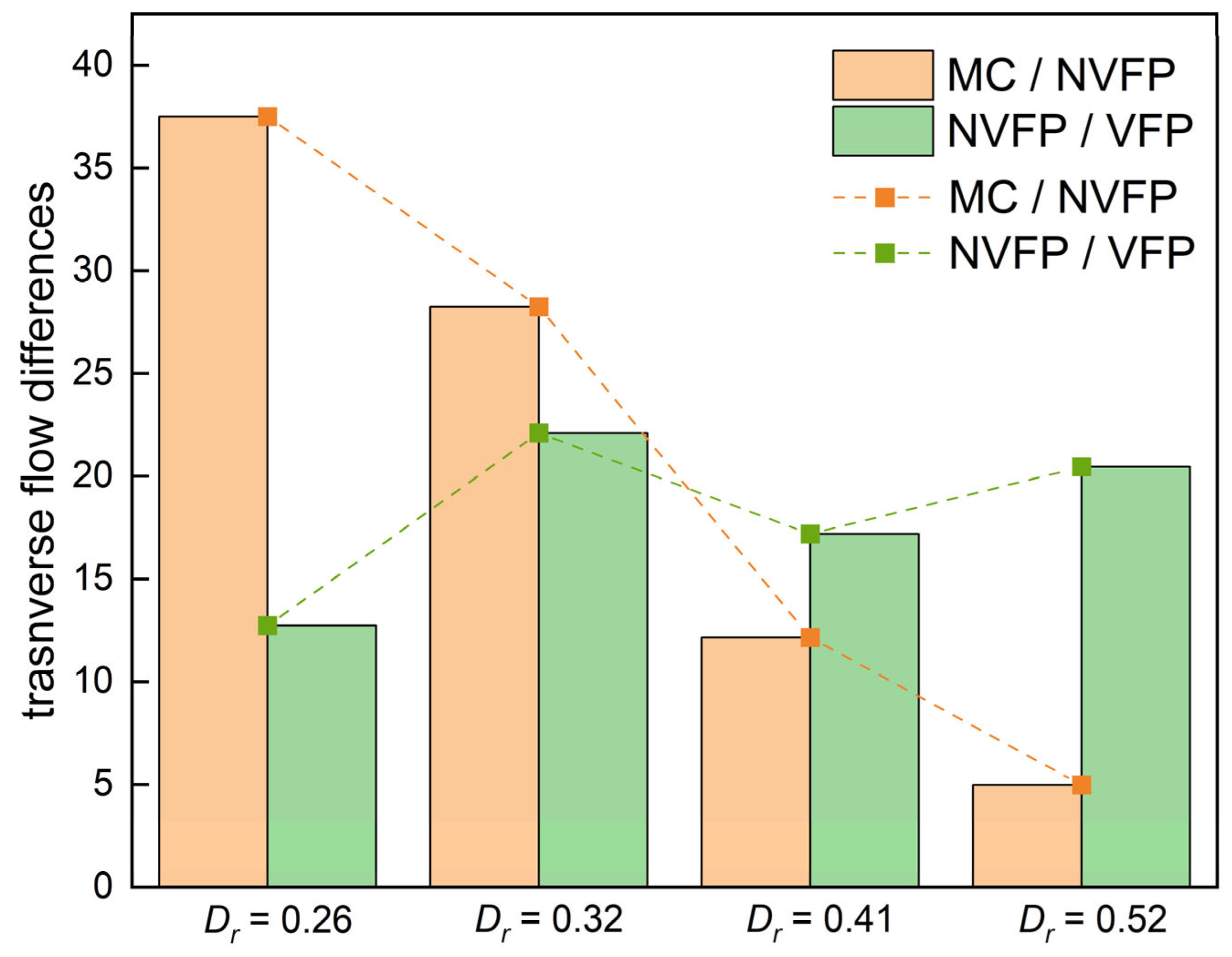
Figure 10 shows the zonal-averaged transverse flow, indicating that as water depth increases, the difference in transverse velocity between the main channel and floodplain diminishes. This implies a reduced spanwise velocity gradient and weakened momentum exchange at higher water depths, thereby lowering velocities in the main channel and boosting velocities on the floodplain—consistent with Section 4.1.

4.4. Power Spectral Density Analysis

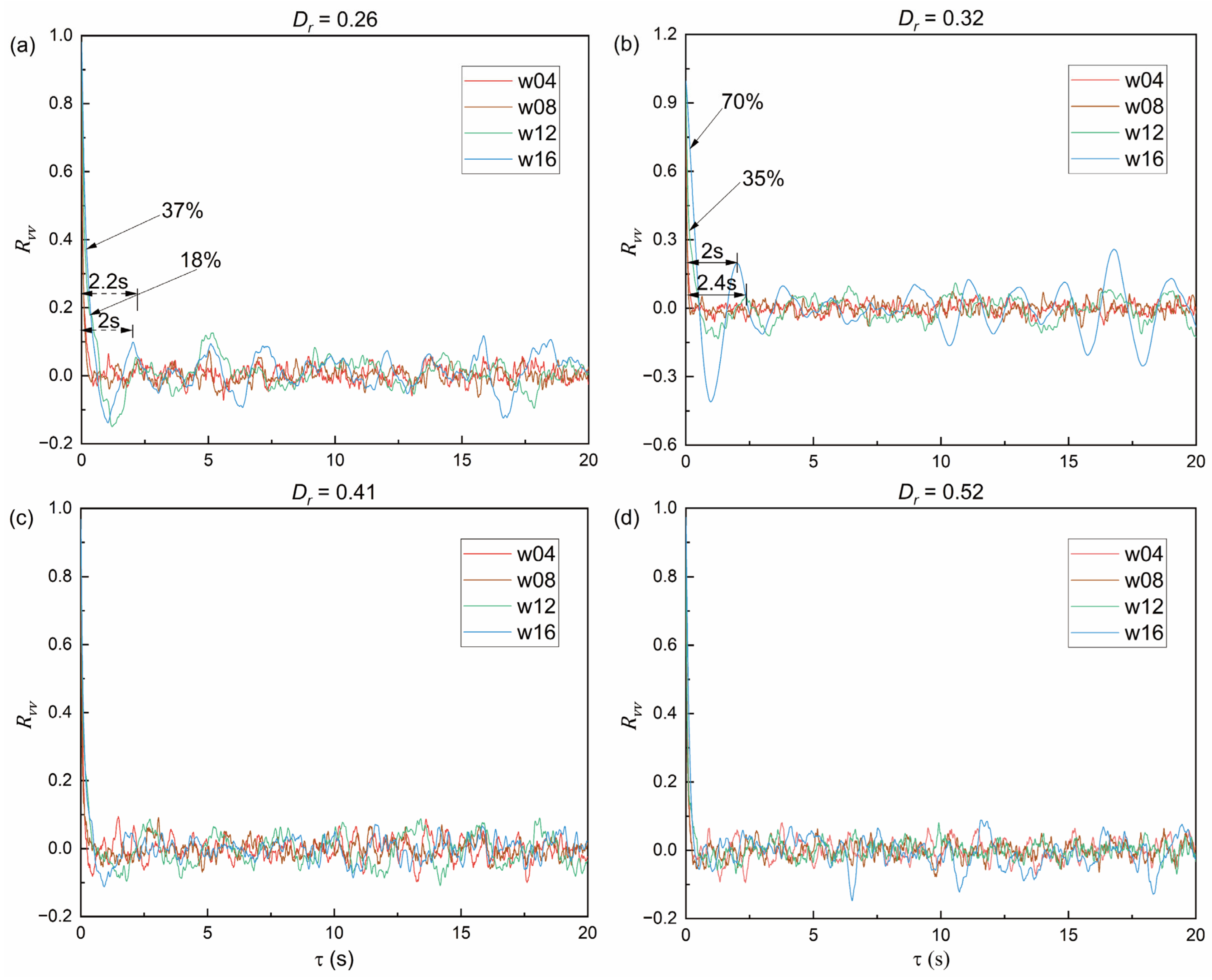
This section examines the power spectral density (PSD) and normalized temporal autocorrelation of the spanwise velocity fluctuations, $v^{\prime }$, to characterize the temporal scales and coherent motions within the flow. Following the methodology described in Section 3.3, a distinct spectral peak combined with a slowly decaying and oscillatory autocorrelation function was interpreted as evidence consistent with long-lived coherent motions. The −5/3 and −3 spectral slopes were used as reference scalings associated with inertial-range and quasi-two-dimensional or enstrophy-dominated dynamics, respectively. However, these spectral slopes were not treated as standalone proof of either three-dimensional or two-dimensional turbulence. Figure 11 shows the PSDs at representative locations for the different depth ratios, while Figure 12 presents the corresponding temporal autocorrelation functions.

For $D_r=0.26$ and 0.32, the spectra at w12 and w16 exhibited a distinct intermediate-frequency peak followed by an approximately −3 spectral decay (Figure 11a,b). The corresponding autocorrelation functions decayed relatively slowly and displayed oscillatory modulation (Figure 12a,b). Taken together, these features are consistent with long-lived, quasi-two-dimensional coherent motions in the vicinity of the NVV shear layer. This finding is broadly consistent with the coherent vortices previously observed near the NVV interface by Zhang and Hu [19]. Comparable signatures were not evident at w08, which represents the vicinity of the MCFP shear layer. Therefore, within the spatial and temporal resolution of the present measurements, coherent activity was more readily detected near the NVV interface than near the MCFP interface under the shallow-flow conditions.

At $D_r=0.41$ and 0.52, the distinct spectral peaks and long-lived autocorrelation modulations at w12 and w16 became substantially weaker or were no longer evident (Figure 11c,d and Figure 12c,d). This observation indicates that the contribution of temporally coherent, large-scale spanwise motions at the sampled locations decreased as the depth ratio increased. The change may be associated with weaker lateral shear, an increased contribution from three-dimensional or canopy-scale turbulence, or a combination of these effects.

In the high-frequency range, the spectrum at w04 generally approached a −5/3 slope, consistent with inertial-subrange scaling [18]. At several other locations, the high-frequency spectral decay was closer to −3. These differences indicate that the organization and scale-to-scale transfer of turbulent fluctuations varied laterally across the compound channel. Although the approximately −3 slope is consistent with turbulence influenced by quasi-two-dimensional coherent motions or strong shear-layer organization [19,36], the spectral slope alone does not uniquely identify the energy-transfer mechanism. Therefore, the steeper spectral decay cannot, by itself, demonstrate that vegetation generated more vortices or produced a higher energy-dissipation rate.

The autocorrelation functions decreased rapidly at small values of $\tau$ at w04 and w08 for all depth ratios and at w12 and w16 for $D_r=0.41$ and 0.52. This rapid initial decay indicates a substantial contribution from rapidly decorrelating, small-scale velocity fluctuations [36], but does not by itself establish that these motions were three-dimensional. In contrast, after the initial decay, the autocorrelation functions at w12 and w16 for $D_r=0.26$ and 0.32 exhibited a more slowly decaying and oscillatory component. This behavior provides additional evidence of long-lived coherent motions near the NVV interface under the shallow-flow conditions.

Using the autocorrelation-based scale-separation procedure described in Section 3.3, the first distinct shoulder or inflection following the rapid initial decay was taken as the transition between the rapidly decorrelating and long-time-correlated components. Under the assumed two-scale decomposition, the value of $R_{vv}$ at this transition provides an approximate estimate of the fraction of spanwise velocity variance associated with long-time-correlated motions. At w12 and w16, the estimated fractions were approximately 18% and 37%, respectively, for $D_r=0.26$, and approximately 35% and 70%, respectively, for $D_r=0.32$. These results indicate that the long-time-correlated component of the spanwise velocity fluctuations was most pronounced near the NVV interface among the investigated locations. These percentages represent estimated fractions of ${v^{\prime }}^2$, rather than fractions of the total turbulent kinetic energy, and depend on the selected transition lag.

For comparison, characteristic time scales of approximately 0.5 s for small-scale turbulence and 2–2.4 s for large-scale coherent motions have been reported in vegetated compound-channel flows [53]. The slowly varying modulation observed at w12 and w16 under the shallow-flow conditions was consistent with the longer time scale associated with large horizontal coherent structures. Within the main channel, the amplitude of the autocorrelation modulation decreased, and the autocorrelation function generally decayed more rapidly with increasing distance from the NVV interface, indicating a progressive weakening of the detectable long-time-correlated component.

Although two mean shear layers were identified from the lateral velocity distributions, the spectral and autocorrelation results revealed only one dominant coherent-motion signature near the NVV interface under the shallow-flow conditions. The measurements do not demonstrate that an MCFP-associated vortex was displaced toward the floodplain or that two initially separate structures merged. A more conservative interpretation is that the NVV shear layer produced the dominant detectable coherent fluctuations at the investigated cross-section, whereas any coherent motion associated with the MCFP interface was weaker, was not captured at w08, or was below the detection capability of the present measurement arrangement.

5. Conclusions

Laboratory experiments were conducted to investigate the effects of the depth ratio, $D_r$, on the flow structure of an asymmetric compound channel with a partially vegetated floodplain. Five cases covering $D_r=0.15-0.52$ were examined. The principal conclusions are as follows.

1. Partial-width vegetation produced two coexisting lateral shear layers: the conventional main-channel/floodplain (MCFP) shear layer and an additional non-vegetated/vegetated-floodplain (NVV) shear layer generated by the discontinuity in vegetation drag. Increasing $D_r$ progressively redistributed streamwise velocity and discharge from the main channel toward the floodplain. The normalized ambient velocity $U_1/U_0$ in the main channel decreased from 1.055 to 0.964, whereas $U_2/U_0$ in the non-vegetated floodplain and $U_3/U_0$ in the vegetated floodplain increased from 0.277 to 0.848 and from 0.041 to 0.441, respectively. Correspondingly, the main-channel discharge fraction decreased from 83.7% to 56.6%, while the combined floodplain contribution increased from 16.31% to 43.33%.

2. The two shear layers responded differently to increasing $D_r$. The dimensionless velocity contrast across the MCFP interface, ${\lambda }_{MCFP}$, decreased from 0.584 to 0.064, representing an approximately 89% reduction. Although ${\lambda }_{NVV}$ also decreased, from 0.741 to 0.316, it remained greater than ${\lambda }_{MCFP}$ in all five cases. From $D_r=0.32$ onward, the absolute velocity difference across the NVV interface also exceeded that across the MCFP interface. Thus, increasing $D_r$ strongly weakened the conventional MCFP shear layer, whereas the vegetation boundary retained a substantial relative velocity contrast. The nominal and momentum thicknesses of the two shear layers varied non-monotonically, indicating that changes in shear intensity did not translate directly into proportional changes in shear-layer width.

3. The vertical velocity profiles also exhibited region-dependent responses to $D_r$. As $D_r$ increased, normalized velocity generally decreased in the main channel but increased in both floodplain regions. The elevation of the maximum main-channel streamwise velocity shifted upward from approximately 5.0 to 8.8 cm. In addition, the velocity measured at approximately 0.25H provided a close estimate of the local depth-averaged velocity, with a mean absolute error of 2.25% and errors below 5% for 26 of the 28 evaluated profiles.

4. In the four ADV-measured cases, the maximum local Reynolds shear stress occurred near the NVV interface rather than at the conventional MCFP interface. This indicates that the vegetation boundary controlled the location of the strongest local turbulent momentum exchange. Nevertheless, local turbulent exchange must be distinguished from the mechanism governing the total depth-averaged transverse momentum transfer. The case-wise maximum absolute magnitude of the mean transverse-advection contribution ranged from 40.84 to 73.96 and exceeded the corresponding maxima of the Reynolds-stress and dispersive-stress contributions by factors of 71.4–356.3 and 74.2–556.7, respectively. Mean transverse advection therefore dominated the total depth-averaged transverse momentum exchange.

5. Power spectral density analysis indicated that energetic large-scale coherent motions over the floodplain were most evident under shallow-flow conditions and weakened as $D_r$ increased. These spectral changes were consistent with the depth-dependent redistribution of velocity contrasts and shear-layer activity. However, because complete cross-sectional secondary-circulation cells were not directly resolved, the observed velocity and dispersive-stress patterns should be interpreted as secondary-flow-related signatures rather than direct measurements of complete circulation structures.

Overall, the results demonstrate that the effect of $D_r$ in a partially vegetated compound channel cannot be characterized solely through the conventional MCFP shear layer. Instead, $D_r$ regulates the relative roles of two coexisting lateral shear layers: the NVV interface determines where local turbulent momentum exchange is strongest, whereas mean transverse advection governs the total depth-averaged exchange. These findings provide a quantitative basis for improving the representation of velocity redistribution and transverse momentum exchange in hydraulic models of partially vegetated compound channels.

References

1. Tang, X. A mixing-length-scale-based analytical model for predicting velocity profiles of open-channel flows with submerged rigid vegetation. Water Environ. J. 2019, 33, 610–619. [Google Scholar]
2. Guan, Y.; Tang, X.; Zhang, Y. The Impact of Double-layered Rigid Vegetation on Flow Structure. In In Proceedings of the 9th International Symposium on Environmental Hydraulics, Seoul, Republic of Korea, 18–22 July 2021; pp. 124–125. [Google Scholar]
3. Nepf, H.; Vivoni, E. Flow structure in depth-limited, vegetated flow. J. Geophys. Res. Ocean. 2000, 105, 28547–28557. [Google Scholar] [CrossRef]
4. Guan, Y.; Tang, X. Influence of Partially-Covered Riparian Vegetation on Flow in a Compound Channel. In Hydraulic and Civil Engineering Technology VII; IOS Press: Amsterdam, The Netherlands, 2022; pp. 934–939. [Google Scholar]
5. Tang, X.; Guan, Y.; Hu, Y. Impact of Different Vegetation Zones on the Velocity and Discharge of Open-Channel Flow. In Proceedings of the 6th International Technical Conference on Frontiers of Hydraulic and Civil Engineering Technology (HCET 2021), Sanya, China, 28–29 August 2021; pp. 486–492. [Google Scholar]
6. Dupuis, V.; Proust, S.; Berni, C.; Paquier, A. Mixing layer development in compound channel flows with submerged and emergent rigid vegetation over the floodplains. Exp. Fluids 2017, 58, 30. [Google Scholar] [CrossRef]
7. Bhagat, C.; Kumar, P.; Sharma, A. Experimental investigation of 3D flow structure and turbulence in a double-layered partially vegetated mobile bed channel. Adv. Water Resour. 2026, 216, 105408. [Google Scholar] [CrossRef]
8. Nezu, I.; Onitsuka, K.; Iketani, K. Coherent horizontal vortices in compound open-channel flows. In Hydraulic Modeling; Seo, I.W., Sonu, J.H., Singh, V.P., Eds.; Water Resources Publications: Lone Tree, CO, USA, 1999; pp. 17–32. [Google Scholar]
9. Stocchino, A.; Brocchini, M. Horizontal mixing of quasi-uniform straight compound channel flows. J. Fluid Mech. 2010, 643, 425–435. [Google Scholar] [CrossRef]
10. Proust, S.; Nikora, V.I. Compound open-channel flows: Effects of transverse currents on the flow structure. J. Fluid Mech. 2020, 885, A24. [Google Scholar]
11. Ackers, P. Flow formulae for straight two-stage channels. J. Hydraul. Res. 1993, 31, 509–531. [Google Scholar] [CrossRef]
12. Proust, S.; Fernandes, J.N.; Leal, J.B.; Rivière, N.; Peltier, Y. Mixing layer and coherent structures in compound channel flows: Effects of transverse flow, velocity ratio, and vertical confinement. Water Resour. Res. 2017, 53, 3387–3406. [Google Scholar] [CrossRef]
13. Juez, C.; Schärer, C.; Jenny, H.; Schleiss, A.J.; Franca, M.J. Floodplain Land Cover and Flow Hydrodynamic Control of Overbank Sedimentation in Compound Channel Flows. Water Resour. Res. 2019, 55, 9072–9091. [Google Scholar] [CrossRef]
14. de Oliveira, L.E.D.; Janzen, J.G.; Folke, F.; Wittmann, F.; Huber, N.P.; Franca, M.J.; Gualtieri, C. Hydrodynamics of Four Moments in the Life of a Floodplain Forest in Compound Channels. Water Resour. Res. 2026, 62, e2024WR038968. [Google Scholar] [CrossRef]
15. Jirka, G.H. Large scale flow structures and mixing processes in shallow flows. J. Hydraul. Res. 2001, 39, 567–573. [Google Scholar] [CrossRef]
16. Soldini, L.; Piattella, A.; Mancinelli, A.; Bernetti, R.; Brocchini, M. Macrovortices-induced horizontal mixing in compound channels. Ocean Dyn. 2004, 54, 333–339. [Google Scholar] [CrossRef]
17. Fernandes, J.; Leal, J.; Cardoso, A. Improvement of the lateral distribution method based on the mixing layer theory. Adv. Water Resour. 2014, 69, 159–167. [Google Scholar] [CrossRef]
18. Truong, S.; Uijttewaal, W. Transverse momentum exchange induced by large coherent structures in a vegetated compound channel. Water Resour. Res. 2019, 55, 589–612. [Google Scholar] [CrossRef]
19. Zhang, J.; Hu, R. Turbulence structure in an experimental compound channel with varying coverage of riparian vegetation on the floodplain. J. Hydrol. 2023, 620, 129378. [Google Scholar] [CrossRef]
20. Proust, S.; Berni, C.; Nikora, V.I. Shallow mixing layers over hydraulically smooth bottom in a tilted open channel. J. Fluid Mech. 2022, 951, A17. [Google Scholar] [CrossRef]
21. Zhang, J.; Wang, W.; Shi, H.; Wang, W.-J.; Li, Z.; Xia, Z. Two-zone analysis of velocity profiles in a compound channel with partial artificial vegetation cover. J. Hydrol. 2021, 596, 126147. [Google Scholar] [CrossRef]
22. Tang, X.; Knight, D.W. Lateral distributions of streamwise velocity in compound channels with partially vegetated floodplains. Sci. China Ser. E Technol. Sci. 2009, 52, 3357–3362. [Google Scholar] [CrossRef]
23. Van Rooijen, A.; Lowe, R.; Ghisalberti, M.; Conde-Frias, M.; Tan, L. Predicting current-induced drag in emergent and submerged aquatic vegetation canopies. Front. Mar. Sci. 2018, 5, 449. [Google Scholar] [CrossRef]
24. Van Prooijen, B.C.; Battjes, J.A.; Uijttewaal, W.S. Momentum exchange in straight uniform compound channel flow. J. Hydraul. Eng. 2005, 131, 175–183. [Google Scholar] [CrossRef]
25. Dorcheh, S.A.M. Effect of Rigid Vegetation on the Velocity, Turbulence, and Wave Structure in Open Channel Flows; Cardiff University: Cardiff, UK, 2007. [Google Scholar]
26. Hamidifar, H.; Keshavarzi, A.; Omid, M.H. Evaluation of 1-D and 2-D models for discharge prediction in straight compound channels with smooth and rough floodplain. Flow Meas. Instrum. 2016, 49, 63–69. [Google Scholar] [CrossRef]
27. Nortek. The Comprehensive Manual for Velocimeters; Nortek AS: Rud, Norway, 2022. [Google Scholar]
28. Goring, D.G.; Nikora, V.I. Despiking acoustic Doppler velocimeter data. J. Hydraul. Eng. 2002, 128, 117–126. [Google Scholar] [CrossRef]
29. Wahl, T.L. Discussion of “Despiking acoustic doppler velocimeter data” by Derek G. Goring and Vladimir I. Nikora. J. Hydraul. Eng. 2003, 129, 484–487. [Google Scholar] [CrossRef]
30. Zampiron, A. Hydraulic Resistance and Flow Structure in Open-Channel Flow Over Streamwise Ridges; University of Aberdeen: Scotland, UK, 2019. [Google Scholar]
31. Caroppi, G.; Vastila, K.; Jarvela, J.; Rowinski, P.M.; Giugni, M. Turbulence at water-vegetation interface in open channel flow: Experiments with natural-like plants. Adv. Water Resour. 2019, 127, 180–191. [Google Scholar] [CrossRef]
32. Unigarro Villota, S.; Ghisalberti, M.; Philip, J.; Branson, P. Characterizing the Three-Dimensional Flow in Partially Vegetated Channels. Water Resour. Res. 2023, 59, e2022WR032570. [Google Scholar] [CrossRef]
33. Ghisalberti, M.; Nepf, H.M. The limited growth of vegetated shear layers. Water Resour. Res. 2004, 40, W07502. [Google Scholar] [CrossRef]
34. White, B.L.; Nepf, H.M. A vortex-based model of velocity and shear stress in a partially vegetated shallow channel. Water Resour. Res. 2008, 44, W01412. [Google Scholar] [CrossRef]
35. Yang, J.Q.; Kerger, F.; Nepf, H.M. Estimation of the bed shear stress in vegetated and bare channels with smooth beds. Water Resour. Res. 2015, 51, 3647–3663. [Google Scholar] [CrossRef]
36. Uijttewaal, W.; Booij, R. Effects of shallowness on the development of free-surface mixing layers. Phys. Fluids 2000, 12, 392–402. [Google Scholar] [CrossRef]
37. Kraichnan, R.H. Inertial ranges in two-dimensional turbulence. Phys. Fluids 1967, 10, 1417–1423. [Google Scholar] [CrossRef]
38. Alexakis, A.; Biferale, L. Cascades and transitions in turbulent flows. Phys. Rep. 2018, 767–769, 1–101. [Google Scholar] [CrossRef]
39. Shiono, K.; Knight, D. Two-dimensional analytical solution for a compound channel. In Proceedings of 3rd International Symposium on Refined Flow Modelling and Turbulence Measurements; Universal Academy Press: Tokyo, Japan, 1988; pp. 503–510. [Google Scholar]
40. Yang, S.Q.; Tan, S.K.; Lim, S.Y. Velocity distribution and dip-phenomenon in smooth uniform open channel flows. J. Hydraul. Eng. 2004, 130, 1179–1186. [Google Scholar] [CrossRef]
41. Kundu, S. Prediction of Velocity-Dip-Position at the Central Section of Open Channels using Entropy Theory. J. Appl. Fluid Mech. 2017, 10, 221–229. [Google Scholar] [CrossRef]
42. Cardoso, A.; Graf, W.H.; Gust, G. Uniform flow in a smooth open channel. J. Hydraul. Res. 1989, 27, 603–616. [Google Scholar] [CrossRef]
43. Nezu, I.; Nakagawa, H.; Jirka, G.H. Turbulence in open-channel flows. J. Hydraul. Eng. 1994, 120, 1235–1237. [Google Scholar] [CrossRef]
44. Shinneeb, A.-M.; Nasif, G.; Balachandar, R. Effect of the aspect ratio on the velocity field of a straight open-channel flow. Phys. Fluids 2021, 33, 085110. [Google Scholar] [CrossRef]
45. Raupach, M.R.; Finnigan, J.; Brunet, Y. Coherent eddies and turbulence in vegetation canopies: The mixing-layer analogy. In Boundary-Layer Meteorology 25th Anniversary Volume, 1970–1995; Springer: Berlin/Heidelberg, Germany, 1996; pp. 351–382. [Google Scholar]
46. Nezu, I.; Sanjou, M. Turburence structure and coherent motion in vegetated canopy open-channel flows. J. Hydro-Environ. Res. 2008, 2, 62–90. [Google Scholar] [CrossRef]
47. Rahimi, H.R.; Tang, X.; Singh, P.; Li, M.; Alaghmand, S. Open channel flow within and above a layered vegetation: Experiments and first-order closure modeling. Adv. Water Resour. 2020, 137, 103527. [Google Scholar] [CrossRef]
48. Poggi, D.; Porporato, A.; Ridolfi, L.; Albertson, J.; Katul, G. The effect of vegetation density on canopy sub-layer turbulence. Bound.-Layer Meteorol. 2004, 111, 565–587. [Google Scholar] [CrossRef]
49. Liu, C.; Shan, Y.; Sun, W.; Yan, C.; Yang, K. An open channel with an emergent vegetation patch: Predicting the longitudinal profiles of velocities based on exponential decay. J. Hydrol. 2020, 582, 124429. [Google Scholar] [CrossRef]
50. Carling, P.A.; Cao, Z.X.; Holland, M.J.; Ervine, D.A.; Babaeyan-Koopaei, K. Turbulent flow across a natural compound channel. Water Resour. Res. 2002, 38, 6-1–6-11. [Google Scholar] [CrossRef]
51. Ikeda, S.; McEwan, I.K. Flow and Sediment Transport in Compound Channels: The Experience of Japanese and UK Research; CRC Press: Boca Raton, FL, USA, 2009. [Google Scholar]
52. Singh, P. An Experimental Study on Turbulent Flow in Asymmetric Compound Channels; University of Liverpool: Liverpool, UK, 2022. [Google Scholar]
53. Truong, S.; Uijttewaal, W. Cycloid flows induced by the Large horizontal coherent structures in the vegetated compound channel. In Proceedings of the E3S Web of Conferences; EDP Sciences: Les Ulis, France, 2018; p. 02045. [Google Scholar]
Figure 1. Experimental setup and measurement arrangement (not to scale). (a) Three-dimensional schematic of the flume. (b) Schematic transverse distribution of the mean streamwise velocity and arrangement of the vertical measurement points. (c) Plan view of the experimental flume. (d) Legend for the symbols used in schematics. (e) Photograph of the experimental facility. (f) Two-row arrangement of the cylindrical stems. The arrows indicate the positive coordinate directions and the streamwise flow direction. The main channel is shaded light blue, the floodplain is shaded light beige, and the vegetated zone is shown in green.
Water 18 01895 g001
Figure 2. Lateral distributions of (a) the normalized depth-averaged streamwise velocity, U d / U 0 ; (b) the transverse gradient of the depth-averaged streamwise velocity, d U d / d y ; and (c) the cross-sectional geometry and boundaries of the main channel, non-vegetated floodplain, and vegetated floodplain for the five depth-ratio cases.
Water 18 01895 g002
Figure 3. Variations with the depth ratio, D r , of (a) the normalized ambient velocities, U 1 / U 0 , U 2 / U 0 and U 3 / U 0 ; and (b) the dimensionless shear parameters, λ M C F P and λ N V V , for the investigated cases.
Water 18 01895 g003
Figure 4. Normalized zonal discharges conveyed by the MC, NVFP, and VFP under different depth ratios. Increasing Dr progressively reduces the MC contribution and increases the combined contribution of the floodplain.
Water 18 01895 g004
Figure 5. Comparison of the zone-averaged vertical profiles of normalized streamwise velocity, U/U0, for the five depth ratios in the (a) main channel (MC), (b) non-vegetated floodplain (NVFP), and (c) vegetated floodplain (VFP). Due to limited vertical measurement points on the floodplain, Dr = 0.15 was excluded in the NVFP and VFP profile. Increasing Dr generally reduced U/U0 in the MC while increasing it in both floodplain regions.
Water 18 01895 g005
Figure 6. Vertical profiles of streamwise velocity at individual lateral measurement positions for (a) D r = 0.32 and (b) D r = 0.52 . The orange, blue, and green profiles represent measurements in the MC, NVFP, and VFP, respectively. The filled magenta symbols mark the elevations at which the local streamwise velocity equals the corresponding depth-averaged velocity. The dotted line in purple indicates the vegetation top, the dash-dotted line in orange indicates the floodplain-bed elevation, and the horizontal dashed lines indicate the zone-averaged equivalent elevations.
Water 18 01895 g006
Figure 7. Vertical velocity profile by the study of Carling, Cao, Holland, Ervine and Babaeyan-Koopaei [50].
Water 18 01895 g007
Figure 8. Distributions of lateral momentum exchange: (a) normalized Reynolds stress contribution; (b) normalized dispersive contribution; (c) normalized transverse-advection contribution.
Water 18 01895 g008
Figure 9. Cross-sectional distributions of normalized Reynolds stress ( u v ¯ ) / u 2 .
Water 18 01895 g009
Figure 10. The difference between the zonal-averaged normalized transverse flow.
Water 18 01895 g010
Figure 11. Power spectral density at typical locations: (a) D r = 0.26, (b) D r = 0.32, (c) D r = 0.41, and (d) D r = 0.52.
Water 18 01895 g011
Figure 12. Temporal autocorrelation function of spanwise velocity fluctuations v : (a) D r = 0.26, (b) D r = 0.32, (c) D r = 0.41, and (d) D r = 0.52.
Water 18 01895 g012