HLS-Based Assessment of Suspended Sediment Concentration in the Middle and Lower Reaches of Liaohe River

Abstract

High-frequency monitoring of suspended sediment concentration (SSC) is important for sustainable river management, but conventional cross-sectional measurements and single-sensor satellite observations cannot simultaneously provide fine spatial detail and sufficient temporal continuity. This study evaluated whether Harmonized Landsat and Sentinel-2 (HLS) observations can improve SSC monitoring in the middle and lower Liaohe River, China. Daily mean cross-sectional SSC records from five hydrological stations were matched with same-day HLS L30 and S30 surface reflectance observations during the ice-free months from 2016 to 2022. Three Ridge regression schemes, including L30-only, S30-only and L30 + S30 fusion models, were assessed using date-grouped cross-validation, temporal extrapolation, station extrapolation and quality-based reliability labeling. The fusion model achieved an out-of-fold RMSE of 0.329, MAE of 0.245 and R² of 0.454 on the log10(SSC) scale, with negligible bias and no clear accuracy degradation relative to the best single-sensor schemes within sensor-specific subsets. The L30–S30 union increased valid observation days by 64.6% compared with the single sensor with a greater number of valid observation days at each station and raised station-month availability to 87.9%. Reliability labels based on clear-water pixel number and proportion helped identify lower-error observations, while spatial transferability varied more substantially among stations than temporal extrapolation. These results show that HLS fusion improves the temporal availability of quality-screened SSC observations in medium-width rivers, although uncertainty remains greater at the extremes of the SSC range and when the model is transferred to new cross-sections.

1. Introduction

Suspended sediment concentration (SSC) is a key physical parameter for evaluating river health, managing water resources, and understanding surface processes [1]. Human management can alter suspended sediment characteristics [2], while satellite observations combined with data-driven models have been applied to estimate SSC in aquatic environments [3]. Its transport and deposition processes more directly shape riverbed morphology and are closely related to channel erosion–deposition dynamics, navigation safety, and the service life and operation of engineering facilities such as reservoirs and ports [4]. Especially in river basins jointly affected by climate change and human activities, strong daily and even hourly fluctuations in SSC are often closely coupled with extreme weather events such as heavy rainfall and floods [5]. Although conventional hydrological station observations at cross-sections can provide high-frequency point-based SSC data, their spatial representativeness is limited, making it difficult to capture the spatiotemporal heterogeneity of water–sediment processes over an entire river reach. Therefore, there is an urgent need to develop high-frequency monitoring techniques with spatiotemporal continuity for watershed water–sediment management and scientific research [6].

This study focuses on the Liaohe River, an important river in northeastern China and one of the seven major rivers in China. The middle and lower reaches of the Liaohe mainstream are located in a temperate monsoon climate zone, where precipitation is highly unevenly distributed throughout the year and heavy rainfall occurs frequently during the summer flood season. This often causes rapid increases in runoff and sediment transport within a short period, resulting in typical event-driven fluctuations in SSC [7]. Meanwhile, some sections of this river reach are sensitive to sediment deposition, where water–sediment processes interact strongly with riverbed erosion and deposition adjustments, posing challenges to sediment management and aquatic environmental protection in the basin [8]. Although hydrological stations such as Tieling, Mahushan, and Pinganbao along the river have accumulated valuable daily observations and provided a basis for understanding changes in cross-sectional water–sediment fluxes, there is still an urgent need for a remote sensing monitoring approach that can balance spatial continuity and temporal resolution, so as to achieve reliable, verifiable, and high-frequency monitoring of SSC dynamics in key river reaches.

Remote sensing technology, with its advantages of synoptic, rapid, and repetitive observation, has become a core means for large-scale SSC monitoring in water bodies [9]. Over the past few decades, various remote sensing methods for SSC retrieval have been developed, ranging from classical empirical and semi-empirical models to semi-analytical and analytical models based on radiative transfer theory, and more recently to machine learning algorithms, all of which have been applied in different aquatic environments [3,10,11]. However, applying these methods to cross-sectional monitoring in medium-width rivers such as the Liaohe still faces many challenges. On the one hand, the optical properties of river water are complex, being jointly affected by phytoplankton and colored dissolved organic matter (CDOM), and are further complicated by problems such as adjacency effects, mixed pixels, and signal saturation at high concentrations, all of which place higher demands on the robustness of retrieval models [12,13]. On the other hand, the choice of data source always involves a trade-off between temporal resolution and spatial resolution. Sensors with high temporal resolution, such as the Moderate Resolution Imaging Spectroradiometer (MODIS) and the Visible Infrared Imaging Radiometer Suite (VIIRS), generally have coarser spatial resolutions than medium-resolution sensors such as Landsat and Sentinel-2. For inland water quality monitoring, coarse ground sampling distance can make narrow or medium-width rivers difficult to resolve and can increase mixed-pixel and adjacency effects [14,15]. In contrast, sensors with higher spatial resolution, such as the Landsat series, can better meet spatial-scale requirements, but their single-sensor revisit cycle is long (e.g., 16 days). After the effects of cloudy and rainy weather are considered, the number of valid observation days becomes seriously insufficient, making it difficult to capture the daily variation in SSC during critical periods such as the flood season and causing frequent breaks in the time series [16,17].

To alleviate the trade-off between spatial and temporal resolution, the National Aeronautics and Space Administration (NASA) developed the Harmonized Landsat and Sentinel-2 (HLS) surface reflectance product. Through systematic geometric and radiometric harmonization of Landsat 8/9 OLI/OLI-2 and Sentinel-2 A/B MSI observations, HLS provides spatially aligned 30 m L30 and S30 surface reflectance data that can be combined into a denser observation sequence [17]. Although the joint use of Landsat and Sentinel-2 can theoretically shorten the average revisit interval to approximately 2–3 days, nominal acquisition frequency does not directly represent the number of observations that remain usable for inland water SSC retrieval after screening for clouds, cloud shadows, snow and ice, water pixel availability, and reflectance quality [17]. For cross-sectional SSC monitoring in medium-width rivers, several practical questions therefore remain: whether joint L30–S30 modeling introduces an accuracy penalty relative to the corresponding single-sensor models, whether fusion increases the actual number of quality-screened observation days, and how well the resulting model performs across different years and hydrological cross-sections. These issues need to be evaluated together before the practical value of HLS fusion for river SSC monitoring can be established.

Against this background, this study evaluated HLS-based retrieval of daily mean cross-sectional SSC using observations from five hydrological stations in the middle and lower reaches of the Liaohe River during the ice-free months of 2016–2022. Three Ridge regression schemes, including L30-only, S30-only, and L30 + S30 fusion models, were established within a unified feature framework. First, the fusion model was compared with the corresponding single-sensor model within the L30 and S30 subsets, and paired date–block bootstrap tests were used to determine whether fusion caused a measurable loss of retrieval accuracy. Second, the coverage benefit was quantified using quality-screened valid observation days and station-month availability rather than nominal revisit frequency. Third, date-grouped cross-validation, temporal extrapolation, leave-one-station-out validation, and reliability labels based on clear-water pixel number and proportion were combined to evaluate temporal stability, spatial transferability, and retrieval reliability under different water pixel conditions. By jointly assessing accuracy retention, actual observation coverage, spatiotemporal transferability, and reliability classification, this study provides a systematic evaluation framework for HLS-based cross-sectional SSC monitoring in medium-width rivers.

2. Materials and Methods

2.1. Study Area

The Liaohe River Basin is located in the southwestern part of northeastern China and is generally influenced by a temperate monsoon climate, characterized by alternating drought and flood conditions and concentrated precipitation within the year. Previous studies have shown that precipitation in this basin is mainly concentrated in July and August, and heavy rainfall events occur frequently [18]. This study focuses on the middle and lower reaches of the Liaohe mainstream, where water–sediment processes are relatively sensitive to seasonal runoff fluctuations and changes in sediment supply conditions, making this reach suitable for cross-sectional SSC monitoring and validation of remote sensing retrieval.

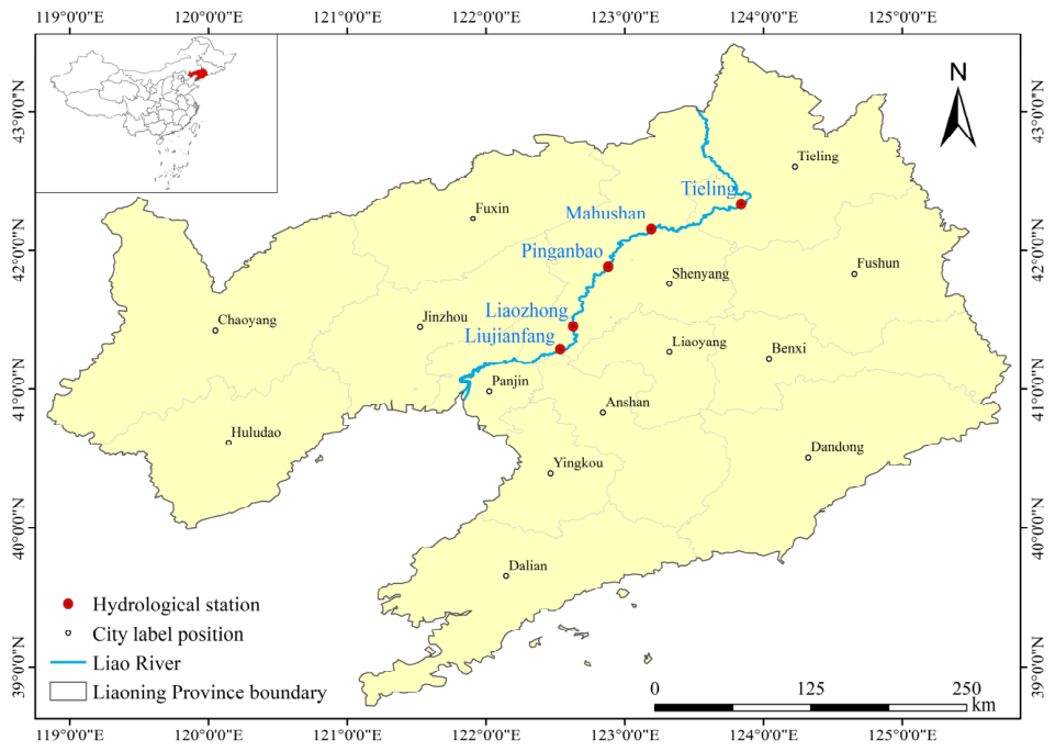
Five hydrological stations with cross-sectional SSC records were selected in this study: Tieling, Mahushan, Pinganbao, Liaozhong, and Liujianfang. All five stations are located in the middle and lower reaches of the Liaohe mainstream and are distributed sequentially from upstream to downstream along the main channel (Figure 1). Representative water surface widths at the station locations were estimated using transects perpendicular to the local river centerline and intersecting the fixed multi-year water mask, and ranged from approximately 90 to 130 m (

Table 1. Reference locations, representative water surface widths, and sample numbers of five hydrological stations.

Station	Station Reference Location		Sample Numbers			Representative Water Surface Width (m)
	Longitude (°E)	Latitude (°N)	L30	S30	Total
Tieling	123.8391	42.3314	46	58	104	90
Mahushan	123.1912	42.1506	55	84	139	130
Pinganbao	122.8807	41.8819	109	173	282	120
Liaozhong	122.6278	41.4523	110	145	255	90
Liujianfang	122.5344	41.2876	114	150	264	100

Note: Representative water surface widths were estimated using transects perpendicular to the local river centerline and intersecting the fixed water mask, and were rounded to the nearest 10 m.

). Shifosi Reservoir is located between the Tieling and Mahushan stations within the study reach. Together, the five stations cover spatial variations in channel morphology and sediment conditions along the mainstream and are used to represent water–sediment characteristics at the cross-sectional scale. Previous studies on sediment deposition in the middle and lower reaches of the Liaohe River have indicated that the reach from Juliuhe to Liujianfang is a significant deposition zone, reflecting strong coupling between water–sediment processes and riverbed erosion–deposition dynamics in this region [19].

To match cross-sectional SSC records from hydrological stations with gridded satellite observations, an 800 m radius region of interest (ROI) was centered on the reference location of each hydrological station. The ROI was used as a local spatial aggregation window rather than as a representation of channel width. The radius was selected to retain a sufficient number of valid water pixels in locally narrow and meandering reaches after quality screening, while reducing sensitivity to single-pixel noise, shoreline mixed pixels, and geometric mismatch between the station locations and satellite pixels, consistent with the use of spatial windows in satellite–in situ matchup validation [20]. Only pixels within the intersection of the ROI and the fixed water mask were included in the spectral statistics. The same ROI definition was applied across all dates and stations to ensure comparability of the extracted remote sensing features under different temporal and hydrological conditions. The study period covered 2016 to 2022. Because winter water body identification and surface reflectance quality are easily affected by snow and ice cover as well as low solar elevation angles, resulting in relatively poor stability, the months from December to February of the following year were excluded from analysis. All subsequent remote sensing feature extraction and sample statistics were conducted for the remaining months.

2.2. Data Acquisition and Sample Construction

2.2.1. HLS v002 Surface Reflectance Data

This study used the HLS surface reflectance product (version v002), and HLS data were obtained through the Google Earth Engine (GEE) platform [21]. In releases from Earth Engine and LP DAAC (Land Processes Distributed Active Archive Center), HLS is provided as two products, HLSL30 (Landsat 8/9) and HLSS30 (Sentinel-2). By applying radiometric and geometric harmonization to Landsat OLI and Sentinel-2 MSI observations, HLS generates a stackable 30 m reflectance time series for near-daily monitoring of land surface and aquatic processes [17]. Although the HLS harmonization procedures reduce geometric and radiometric differences between L30 and S30, residual sensor-specific spectral differences may remain. Therefore, the fusion model included a sensor indicator term, and its performance was evaluated separately within the L30 and S30 subsets. The QA (Quality Assessment) layer in HLS v002 is Fmask-based, with aerosol-level information derived from atmospheric correction, and provides flags for clouds, areas adjacent to clouds or shadows, cloud shadows, snow/ice, water, and aerosol levels [21,22].

2.2.2. In Situ SSC Data

The in situ SSC data used in this study were obtained from the routine suspended sediment monitoring records of the Liaoning Provincial Hydrology Bureau, China. The dataset comprised daily mean cross-sectional SSC records from 2016 to 2022 for the five hydrological stations—Tieling, Mahushan, Pinganbao, Liaozhong, and Liujianfang—with a daily temporal resolution and units of kg m⁻³. Suspended sediment samples were collected using bottle samplers at multiple verticals across each cross-section. Depending on the station, either depth-integrated sampling or one-point sampling at 0.5 of the local water depth was used to determine cross-sectional mean SSC.

Discrete measurements of cross-sectional SSC were used to construct continuous SSC hydrographs, from which daily mean cross-sectional SSC values were derived. For satellite matchup, the daily mean cross-sectional SSC at each station was paired with HLS observations acquired on the same date. Records with missing dates, missing SSC values, or zero SSC were excluded before modeling because log10(0) is undefined. No negative SSC values were present in the final modeling dataset. Unusually high SSC values were checked during data screening but were not removed solely on the basis of magnitude.

2.2.3. Sample Matching and Quality Control

To match the daily mean cross-sectional SSC records with satellite observations at a consistent spatiotemporal scale, each sample was defined as a station–date–sensor record. For a given station and date, if both L30 and S30 observations were available, each sensor observation was separately paired with the corresponding daily mean cross-sectional SSC value and retained as a separate sensor-specific record.

The sample construction procedure was as follows:

First, clouds, adjacent clouds, cloud shadows, snow/ice, and invalid pixels were screened using the HLS QA layer, and multiple scenes acquired by the same sensor on the same date were composited using a quality-based mosaic to generate daily surface reflectance images.

Second, the normalized difference water index (NDWI) was calculated for pixels not excluded by QA in each daily image as follows [23]:

$$NDWI={\displaystyle \frac{\mathit{Green} - NIR}{\mathit{Green} + NIR}}$$

(1)

In this equation, Green and NIR denote surface reflectance in the green and near-infrared bands, corresponding to B3 and to B5 for L30 or B8 for S30, respectively. The theoretical range of NDWI is [−1, 1]. In general, water bodies exhibit relatively high reflectance in the green band and strong absorption in the near-infrared band, and therefore usually have relatively high NDWI values [23]. However, turbidity during the flood season, shoreline mixed pixels, and local geometric mismatch may reduce the NDWI values of actual water pixels in medium-width rivers. A comparison of 52 HLS images showed that using NDWI > 0 retained 22.39% fewer candidate channel water pixels than using NDWI > −0.1. Therefore, NDWI > −0.1 was adopted to reduce water omission and maintain the continuity of the river corridor. Potential false positive identification outside the channel was further constrained using the fixed multi-year water mask described below. The same threshold was also used for water extraction from NDWI_median.

To further suppress false identification outside the river channel and provide a uniform spatial constraint for subsequent sample statistics, a fixed water mask was constructed in this study. Based on the median composite of NDWI during the study period (NDWI_median), long-term stable water candidates were extracted using the threshold NDWI_median > −0.1, and a one-time manual correction was applied to the candidate pixels to preserve a continuous river corridor, thereby generating a fixed water mask used consistently throughout the study period. Subsequently, a circular buffer with a radius of 800 m was generated around each station, and the overlap between the ROI and the fixed water mask was used as the statistical area. The total number of candidate water pixels within this area was denoted as W. On this basis, the number of clear-water pixels on a given day was defined as P, referring to pixels within the statistical area that were not excluded by QA flags for clouds, cloud shadows, snow, or ice and that also satisfied NDWI > −0.1 on that day. The clear-water proportion was then calculated as F = P/W. P and F provide complementary sample-quality constraints: P represents the absolute number of usable water pixels available for spectral aggregation, whereas F represents their relative spatial coverage within the fixed candidate water area. Minimum inclusion thresholds of P ≥ 30 and F ≥ 0.15 were applied before feature extraction. A total of 1136 station–date–sensor records passed this pre-screening and entered the subsequent feature extraction and SSC-matching procedures.

Finally, for records that passed the pixel-level QA, water identification, and P/F pre-screening procedures, the spectral information of valid water pixels within each ROI was statistically aggregated, and the resulting remote sensing features were merged with the cleaned daily SSC records by station and date. Records without matched positive SSC values or with negative median reflectance in the corresponding spectral inputs were excluded. The negative-reflectance check was performed after spectral aggregation and was therefore distinct from the preceding QA, NDWI, and P/F screening procedures. Negative median reflectance was treated as an invalid condition for empirical feature construction because negative surface reflectance values are not physically meaningful and may destabilize ratio and normalized index calculations. No additional upper reflectance threshold was applied. This yielded a total of 1044 samples available for modeling from 2016 to 2022, including 434 L30 samples and 610 S30 samples (Table 1).

2.3. Methods

2.3.1. Feature Construction and Modeling Schemes

To characterize SSC at the cross-sectional scale, the spectral information of valid water pixels that passed quality screening was statistically aggregated within each station window to construct feature vectors at the station–date–sensor scale. Specifically, for water pixels within the ROI that satisfied the quality screening criteria, the median reflectance values of six bands, namely Blue, Green, Red, NIR, SWIR1, and SWIR2, were calculated, and spectral indices and ratio features were further derived on this basis. The input features consisted of three parts: (1) the median reflectance values of six bands (Blue, Green, Red, NIR, SWIR1, and SWIR2), which were used to characterize the shape of the water reflectance spectrum; (2) four spectral index/ratio features derived from the above median band values (NDTI, NDVI, RG = Red/Green, and RN = Red/NIR), which were used to enhance turbidity information and constrain potential interference from non-water or mixed pixels. Among them, NDTI [24] and RG characterize the red–green spectral contrast associated with turbidity variations, whereas NDVI [25] and RN exploit the strong near-infrared absorption of water to help identify non-water or mixed-pixel contamination; RG and RN were used as empirical band ratios in this study. In this study, NDWI was mainly used for water identification and quality control and was not included as an input to the regression model; and (3) a sensor indicator term, is_S30 (S30 = 1, L30 = 0), which was used to absorb systematic differences between L30 and S30, allowing the fusion model to learn cross-sensor offsets within a unified feature space. The formulas and applicable modeling schemes of these features are summarized in

Table 2. Formulas and applicable modeling schemes of input features.

Feature	Formula	Applicable Schemes
Blue	ρBlue	A1/A2/B_all
Green	ρGreen	A1/A2/B_all
Red	ρRed	A1/A2/B_all
NIR	ρNIR	A1/A2/B_all
SWIR1	ρSWIR1	A1/A2/B_all
SWIR2	ρSWIR2	A1/A2/B_all
RG	ρRed/ρGreen	A1/A2/B_all
RN	ρRed/ρNIR	A1/A2/B_all
NDTI	(ρRed − ρGreen)/(ρRed + ρGreen)	A1/A2/B_all
NDVI	(ρNIR − ρRed)/(ρNIR + ρRed)	A1/A2/B_all
is_S30	S30 = 1; L30 = 0	B_all

Notes: ρ denotes the surface reflectance of the corresponding band. is_S30 is the sensor indicator variable. A1, A2, and B_all denote the L30-only, S30-only, and fusion modeling schemes, respectively.

. The daily mean cross-sectional SSC was used as the response variable for model training. Considering the right-skewed distribution of SSC and its potentially wide concentration range, the log10 transformation helps reduce the influence of high-concentration values, alleviate heteroscedasticity, and make the relationship between spectral features and SSC more suitable for empirical linear modeling [26]. Therefore, log10(SSC) was used as the modeling target to improve the fitting stability and error balance of the Ridge regression model.

Each single-sensor scheme, A1 and A2, used 10 spectral predictors, comprising the median reflectance of six bands and four derived indices or ratios, whereas the fusion scheme B_all included the same 10 predictors plus the sensor indicator is_S30, resulting in 11 predictors. Because several indices and ratios were derived from the same spectral bands, appreciable collinearity was expected among the predictors. Under such conditions, ordinary least-squares coefficient estimates may become sensitive to variations in the training samples. Ridge regression was therefore adopted to constrain coefficient magnitudes through an L₂ penalty while retaining the interpretability of a linear model [27]. Ridge remains a linear method and was used in this study as a regularized and interpretable modeling framework rather than as a means of representing arbitrary nonlinear relationships. The L₂ regularization term is defined as follows:

$${‖\beta ‖}_2^2=\sum _{j=1}^D{\beta }_j^2$$

(2)

The objective function of Ridge regression can be expressed as follows:

$$\stackrel{\wedge }{\beta }=\mathit{arg}\underset{\beta }{min}\left\{\sum _{i=1}^n{\left(y_i-x_i^{{\rm T}}\beta \right)}^2+\lambda {‖\beta ‖}_2^2\right\}$$

(3)

where y_i is the observed log10(SSC) of the i-th sample, x_i is the corresponding remote sensing feature vector, λ is the regularization strength parameter, β is the regression coefficient vector, and D denotes the number of input features. For A1 and A2, D = 10, comprising six band-reflectance features and four derived index or ratio features. For B_all, D = 11, because the sensor indicator is_S30 was included in addition to the same 10 spectral features. In each outer cross-validation fold, the feature standardization parameters were estimated using only the outer training set. For a given λ, β was obtained by minimizing Equation (3) on the standardized outer training data. Therefore, the estimated coefficient vector was specific to the training samples and the selected λ, whereas the corresponding outer test fold did not participate in coefficient estimation. To avoid subjective specification of the regularization strength, λ was selected separately within each outer training set using an inner three-fold cross-validation grouped by date. Fifteen logarithmically spaced candidate values ranging from 10⁻³ to 10³ were evaluated. Within each inner split, the feature standardization parameters were estimated using only the inner training subset and were then applied to the corresponding inner validation subset. For each candidate λ, the mean RMSE across the three inner validation folds was calculated, and the value yielding the lowest mean RMSE was selected. Because λ selection was conducted independently within each outer training set, the selected value could differ among the outer folds. After λ had been selected, the feature standardization procedure and the Ridge model were refitted using all samples in the corresponding outer training set, and the resulting model was then applied to the outer test fold.

To quantify the benefits of sensor fusion, three modeling schemes were defined in this study: A1 (L30-only), trained using only L30 samples; A2 (S30-only), trained using only S30 samples; and B_all (Fusion), jointly trained using the combined L30 and S30 samples.

2.3.2. Validation Strategy, Metrics, and Significance Testing

To avoid performance overestimation caused by spatiotemporal correlations among samples, three complementary validation frameworks were adopted to assess model generalization: date-grouped cross-validation, temporal extrapolation validation, and station extrapolation validation. Under the date-grouped cross-validation framework, the 1044 records were divided into five mutually exclusive outer folds using date as the grouping unit, with all records from the same date assigned to the same fold. In each iteration, four folds were used for model training and the remaining fold was used for testing. Each record received one prediction only when it belonged to the held-out outer test fold and had not participated in the corresponding model training. The predictions from the five test folds were then combined to form the complete out-of-fold (OOF) predictions. This design reduced information leakage associated with shared hydrological and atmospheric conditions among records acquired on the same date. Temporal extrapolation validation was conducted by splitting the samples by year, using samples from 2016 to 2020 as the training set and samples from 2021 to 2022 as an independent test set, in order to examine model stability under interannual variation and distributional differences. Station extrapolation validation adopted a leave-one-station-out scheme with five iterations to evaluate the model’s generalization ability at cross-sections not involved in training. All feature standardization, Ridge regularization parameter selection, and model fitting were performed only within the training set and then applied to the corresponding test set.

Model performance was evaluated using RMSE (root mean square error), MAE (mean absolute error), and R² (coefficient of determination). To assess the improvement of the fusion scheme B_all relative to the single-sensor schemes, ΔRMSE was defined as RMSE (baseline)—RMSE (B_all). In fair comparisons within sensor-specific subsets, the baseline was defined as the best corresponding single-sensor scheme, that is, A1 for the L30 subset and A2 for the S30 subset. To evaluate the statistical uncertainty of the differences, a paired bootstrap by date blocks was adopted. Bootstrap is a nonparametric method based on repeated resampling and is used to estimate the sampling distribution and confidence interval of a statistic. In this study, date was used as the resampling unit, with all samples from the same date treated as one block and repeated for B = 5000 times. The 95% confidence interval of ΔRMSE was then obtained; if the confidence interval did not cross 0, the difference was considered statistically significant [28].

To examine whether the performance of the fusion scheme was sensitive to model form, an additional comparison was conducted for B_all using ordinary least squares regression (OLS), Ridge regression, and random forest. All three models used the same 1044 records, the same 11 input features, and the same five date-grouped outer folds. OLS used the same training-fold standardization procedure as Ridge. The random forest was fitted using fixed parameters, including 400 trees, a maximum depth of 20, a minimum split size of 4, a minimum leaf size of 2, square-root feature sampling, and a random seed of 42. Model performance was evaluated using OOF RMSE, MAE, and R². Paired RMSE differences relative to Ridge were further evaluated using the same 5000-replicate date–block bootstrap procedure.

2.3.3. Coverage Statistics and Reliability Classification

The value of multi-source fusion lies not only in retrieval accuracy, but also in the spatiotemporal coverage of available observations and the interpretable reliability of retrieval results. Therefore, this study established a unified framework for evaluation and labeling from two aspects, namely coverage statistics and reliability classification, providing a second line of evidence for the fusion gains presented in Section 3.

Coverage was defined in terms of valid observations available for modeling, and the statistical objects were the samples that passed quality control and were successfully matched with daily mean cross-sectional SSC records. Considering that both L30 and S30 observations may exist on the same date, counting by sample rows would lead to duplicate accumulation. Therefore, the number of observation days was used as the primary metric, while the number of sample rows was used only to describe the modeling dataset.

For any statistical unit g (e.g., the entire study period, station, station-year, or station-month), the following quantities were defined:

N_L30(g): the number of valid observation days for L30 within that unit;

N_S30(g): the number of valid observation days for S30 within that unit;

N_∪(g): the number of fused valid observation days for L30 and S30 within that unit (union);

N_∩(g): the number of same-day dual-source observation days within that unit (intersection).

To quantify the coverage gain brought by fusion, the relative improvement rate was defined as follows:

$$Gain(g)={\displaystyle \frac{N_{\cup }\left(g\right)-\mathit{max}(N_{L30}\left(g\right),N_{S30}\left(g\right))}{\mathit{max}(N_{L30}\left(g\right),N_{S30}\left(g\right))}}$$

(4)

Coverage statistics were analyzed from station-level and monthly scale perspectives. At the station level, N_L30, N_S30, N_∪, and Gain were compared among stations to characterize spatial differences in valid observation coverage. At the monthly scale, station-month availability and the contributions of L30-only, S30-only, and dual-source observations were summarized to examine whether fusion improved temporal continuity.

Although the improvement in coverage increases the number of available samples, image quality and effective water conditions still vary substantially across dates. To provide interpretable quality labels for the retrieval results, an empirical reliability labeling scheme was constructed based on the quality statistics generated during sample construction, with the number of clear-water pixels P and the clear-water proportion F as the core variables. Specifically, P denotes the number of pixels within the overlap between the station ROI and the fixed water mask that were not excluded by QA flags for clouds, cloud shadows, snow, or ice and also satisfied NDWI > −0.1 on that day; F = P/W, where W is the total number of candidate water pixels within that area. The thresholds were determined using an empirical error-anchoring approach: taking the OOF errors from the main experiment (date-grouped cross-validation) as the reference, the variation in the absolute error of individual samples, |ŷ − y|, with P and F was analyzed, where ŷ denotes the model’s OOF prediction for y = log10(SSC).

The thresholds P ≥ 30 and F ≥ 0.15 were used as minimum inclusion criteria before model development. For the 1044 records that passed these criteria and the subsequent SSC and reflectance validity checks, a separate reliability label was assigned based on the OOF error patterns. High reliability was defined as P ≥ 100 and F ≥ 0.5, whereas Mid reliability denoted records that passed the basic inclusion criteria but did not meet both High thresholds. The High/Mid classification was used for reliability interpretation and quality-based application screening; Mid records were not removed from model training or evaluation.

To evaluate the sensitivity of retrieval performance and observation retention to the P and F criteria, the existing B_all OOF predictions were re-evaluated under 12 threshold combinations, with P set to 30, 50, 75, or 100 and F set to 0.15, 0.25, or 0.50. For each combination, the number and proportion of retained records, the number of unique observation dates, RMSE, MAE, and R² were recalculated. The model was not retrained for each threshold combination; instead, the analysis examined how progressively stricter quality screening affected the independently generated OOF errors and observation availability.

3. Results

3.1. Comparison of Model Accuracy and Assessment of Cross-Sensor Consistency

3.1.1. Comparison Within Sensor-Specific Subsets

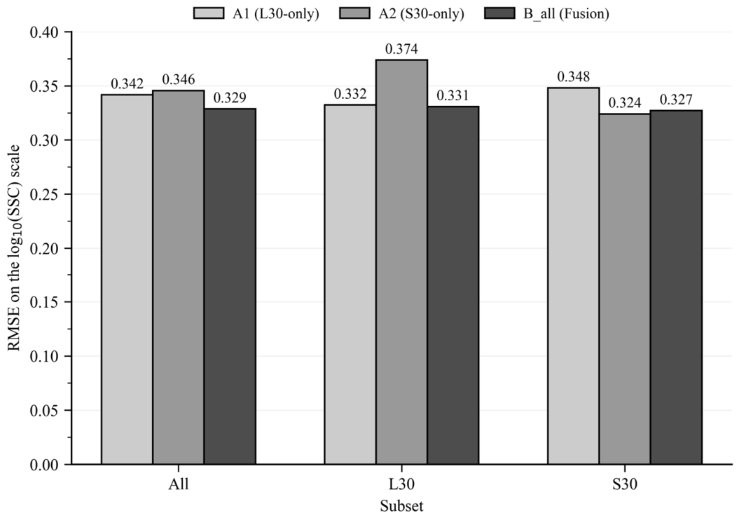
Under five-fold cross-validation grouped by date, the performance metrics of the three schemes on the full sample set, the L30 subset, and the S30 subset are shown in

Table 3. Performance metrics of the three training schemes on different evaluation sets under date-grouped cross-validation (log10 scale).

Subset	Scheme	n	RMSE	MAE	R2	Bias
All	A1 (L30-only)	1044	0.342	0.257	0.410	−0.053
All	A2 (S30-only)	1044	0.346	0.257	0.397	0.019
All	B_all (Fusion)	1044	0.329	0.245	0.454	0.002
L30	A1 (L30-only)	434	0.332	0.244	0.442	0.001
L30	A2 (S30-only)	434	0.374	0.275	0.294	0.041
L30	B_all (Fusion)	434	0.331	0.243	0.447	0.003
S30	A1 (L30-only)	610	0.348	0.267	0.379	−0.092
S30	A2 (S30-only)	610	0.324	0.245	0.462	0.003
S30	B_all (Fusion)	610	0.327	0.246	0.452	0.002

Notes: Bias denotes the mean prediction error; Bias < 0 indicates overall underestimation, whereas Bias > 0 indicates overall overestimation.

. To ensure a consistent comparison basis, sensor-specific subsets were used as the primary units for accuracy comparison in this study: A1 was compared with B_all within the L30 subset, and A2 was compared with B_all within the S30 subset. This design was used to test whether fusion came at the cost of reduced accuracy for the corresponding sensor-specific subset. The related results are shown in Figure 2 and Figure 3.

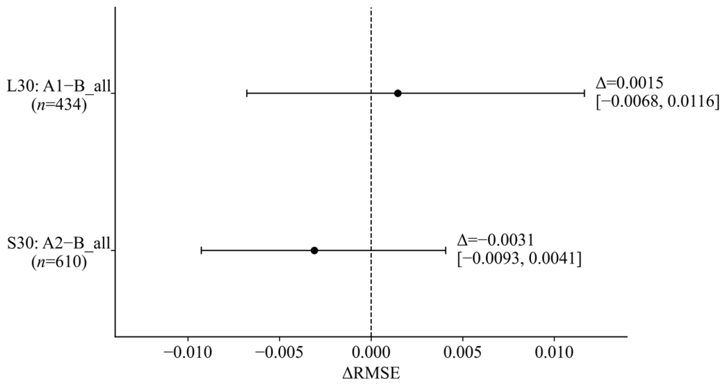
As shown in Table 3 and Figure 2, the error levels of B_all in both the L30 and S30 subsets were close to those of the corresponding best single-sensor models. Fusion gains were further quantified using ΔRMSE = RMSE(baseline) − RMSE(B_all) (Figure 3), with A1 used as the baseline in the L30 subset and A2 used as the baseline in the S30 subset. The 95% confidence intervals of ΔRMSE for both subsets crossed 0, indicating that, under the within-subset comparison framework, the accuracy differences between the fusion and single-sensor schemes were not statistically significant. Therefore, under sensor-specific subset comparisons, the fusion scheme showed error levels in both subsets that were similar to those of the corresponding best single-sensor models.

3.1.2. Cross-Sensor Consistency and Error Structure

Single-sensor models generally perform better within their corresponding sensor-specific subsets, but they tend to degrade under cross-sensor transfer, and the direction of degradation is asymmetric. As shown in Table 3, A1 had lower errors in the L30 subset, but its errors increased in the S30 subset and showed more pronounced underestimation; A2 performed better in the S30 subset, but degraded substantially in the L30 subset and was accompanied by overestimation. In contrast, the fusion scheme B_all showed more balanced error levels across both the L30 and S30 subsets, and its Bias was also closer to 0. This indicates that fusion can mitigate error fluctuations and systematic biases caused by sensor differences, thereby improving cross-sensor consistency and robustness.

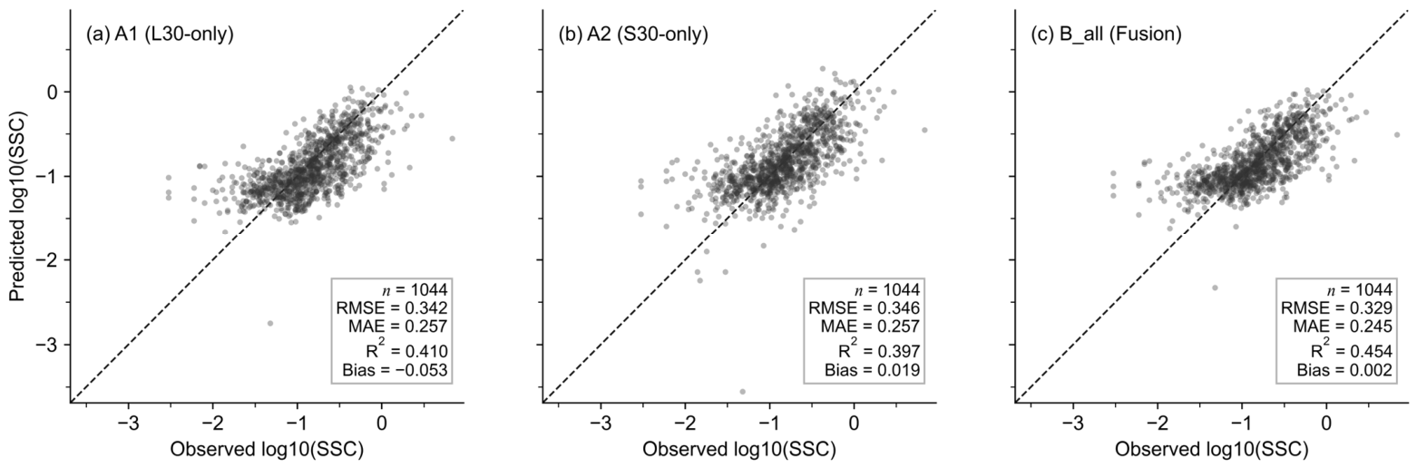
Figure 4 shows the observed-versus-predicted scatterplots of the three schemes for the full sample set. The point clouds of all three schemes are distributed around the 1:1 line, indicating that the models were able to capture SSC variation on the log10 scale. Combined with Table 3 (and the Bias values shown in Figure 4), A1 exhibited a negative Bias, whereas A2 showed a positive Bias, indicating that the two single-sensor models tended toward underestimation and overestimation, respectively, under mixed cross-sensor evaluation conditions. In contrast, the Bias of the fusion scheme B_all was closer to 0, suggesting smaller systematic bias and a more stable error pattern under cross-sensor conditions. However, the predicted values were more concentrated toward the center of the observed range, resulting in some overestimation at low SSC and underestimation at high SSC. These results indicate that B_all captured the overall variation in SSC, although its ability to represent extreme values remained limited.

Overall, the fusion scheme showed no clear evidence of accuracy degradation in comparisons within sensor-specific subsets; under cross-sensor conditions, it exhibited more balanced error levels and systematic bias closer to zero, indicating better cross-sensor consistency and robustness.

As an additional model-form sensitivity test for B_all, OLS and Ridge showed closely comparable OOF performance. OLS achieved an RMSE of 0.327, an MAE of 0.244, and an R² of 0.460, whereas the corresponding values for Ridge were 0.329, 0.245, and 0.454, respectively. The difference defined as RMSE(OLS) − RMSE(Ridge) was −0.002, with a 95% date–block bootstrap confidence interval of [−0.004, 0.001], indicating no statistically significant difference. Random forest produced an RMSE of 0.340, an MAE of 0.254, and an R² of 0.417. Its RMSE difference relative to Ridge was 0.011, with a 95% confidence interval of [0.003, 0.019], indicating a higher error than Ridge. Therefore, the tested nonlinear model did not improve retrieval performance, suggesting that the remaining retrieval errors were not solely attributable to the linear form of Ridge. Ridge was retained as the main model because it provided a regularized and interpretable framework for the correlated spectral predictors.

3.2. Station-Level and Monthly Scale Coverage

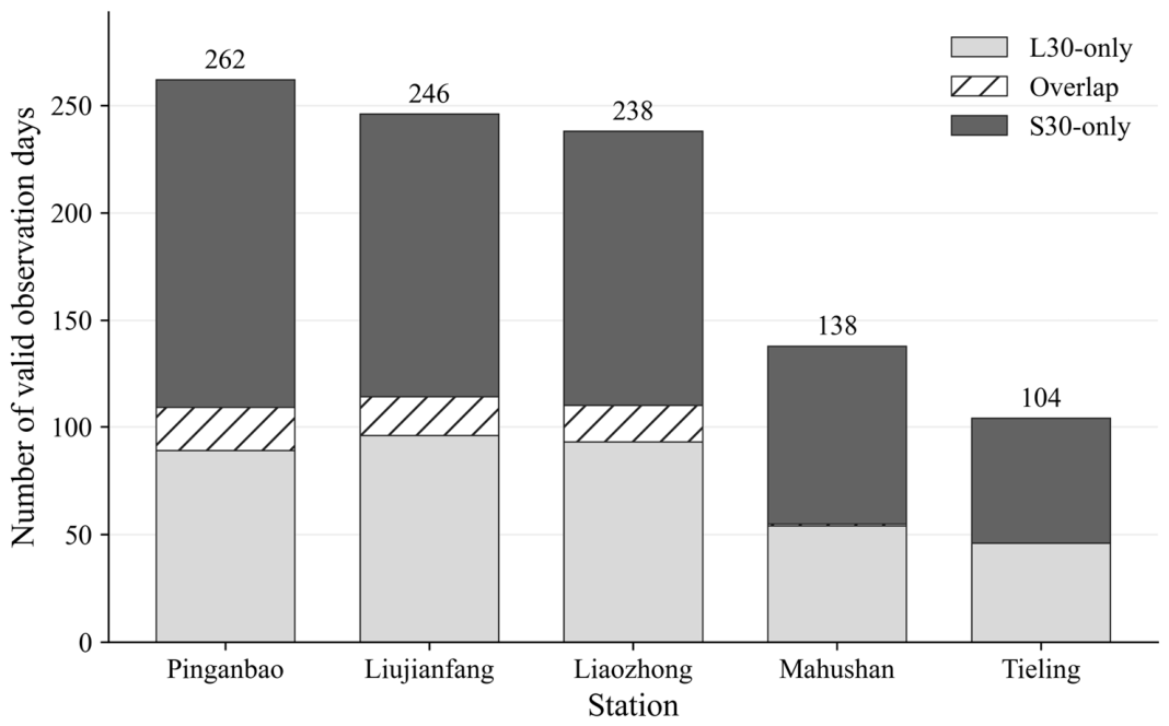
As shown in Figure 5, the number of valid observation days under the fusion scheme (the date-wise union of L30 and S30) was higher than that of either single sensor at all five stations. Based on deduplicated valid observation dates, the union reached 262 days at Pinganbao, 246 days at Liujianfang, 238 days at Liaozhong, 138 days at Mahushan, and 104 days at Tieling. Using the single sensor with the larger number of valid observation days at each station as the baseline, fusion added 46–96 valid observation days, with increases of 96, 93, 89, 54, and 46 days at Liujianfang, Liaozhong, Pinganbao, Mahushan, and Tieling, respectively. The mean relative improvement rate was 0.646 and the median was 0.641, with the highest value at Tieling (0.793) and the lowest at Pinganbao (0.514). Meanwhile, same-day dual-source overlapping observations were only 0–20 days, indicating that the coverage gain mainly came from complementary observations by the two sensors on different dates rather than repeated observations on the same date.

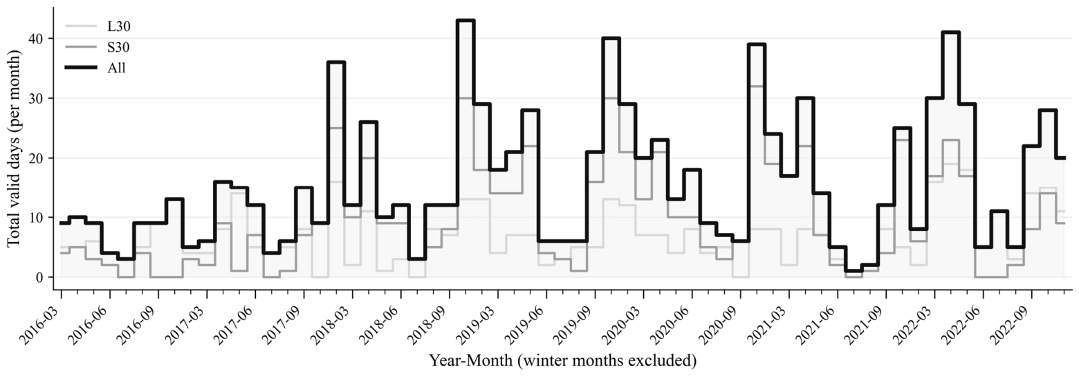
At the monthly scale, “station-month” was used as the statistical unit, yielding a total of 315 combinations during the study period. The fusion union provided valid observations for 277 combinations, accounting for 87.9%, which was higher than that of L30 with 238 combinations (75.6%) and S30 with 217 combinations (68.9%). Among them, 38 combinations lacked observations from both sources; among the remaining 277 combinations with observations, 60 were available only from L30, 39 only from S30, and 178 from both sources, indicating stable complementarity at the monthly scale. As shown in Figure 6, the fusion union (Fusion, L30∪S30) series was generally higher than the single-sensor series, and in months when observations from one sensor were sparse, the other sensor provided supplementary observations, thereby improving the continuity of the monthly time series. Overall, fusion not only increased the number of valid observation days at the station scale, but also improved station-month availability and alleviated temporal gaps at the monthly scale, providing more complete observational support for SSC retrieval and for seasonal and interannual analyses.

3.3. Reliability Classification and Extrapolation Tests

Before reliability classification, the sensitivity of retrieval error and observation retention to the P and F thresholds was evaluated using the existing B_all OOF predictions. As shown in

Table 4. Sensitivity of sample retention and B_all OOF performance to P and F threshold combinations.

P Threshold	F Threshold	Retained Records	Retention (%)	Unique Dates	RMSE	MAE	R2
30	0.15	1044	100.0	342	0.329	0.245	0.454
30	0.25	1011	96.8	333	0.326	0.243	0.455
30	0.50	810	77.6	288	0.320	0.236	0.458
50	0.15	977	93.6	320	0.329	0.245	0.443
50	0.25	974	93.3	319	0.329	0.245	0.443
50	0.50	810	77.6	288	0.320	0.236	0.458
75	0.15	848	81.2	298	0.320	0.238	0.457
75	0.25	848	81.2	298	0.320	0.238	0.457
75	0.50	801	76.7	286	0.319	0.236	0.458
100	0.15	702	67.2	277	0.319	0.233	0.479
100	0.25	702	67.2	277	0.319	0.233	0.479
100	0.50	687	65.8	271	0.321	0.235	0.476

Notes: Under P ≥ 75, increasing the F threshold from 0.15 to 0.25 did not exclude any additional records because all records satisfying P ≥ 75 already met F ≥ 0.25. Therefore, the retained sample size and performance metrics were identical. The same pattern occurred under P ≥ 100.

, the basic thresholds of P ≥ 30 and F ≥ 0.15 retained all 1044 modeling records from 342 unique observation dates, with an RMSE of 0.329. Progressively stricter thresholds reduced RMSE only modestly, with the lowest value being 0.319, whereas the retained proportion decreased to as low as 65.8% and the number of unique dates decreased to 271. Thus, the maximum RMSE reduction was approximately 0.010, accompanied by the loss of up to 34.2% of the records and 71 unique observation dates. These results indicate that, within the evaluated threshold range, the basic thresholds provide a reasonable balance between retrieval error and observation availability, whereas the stricter thresholds are more suitable for reliability classification than for mandatory sample exclusion.

Based on the OOF error patterns and the trade-off identified in Table 4, two reliability labels were assigned to the 1044 records that passed the basic quality control: High, with 687 samples (65.8%), defined by P ≥ 100 and F ≥ 0.5; and Mid, with 357 samples (34.2%), comprising the remaining records that passed the basic quality control. This indicates that even among records passing the basic quality control, effective water conditions still varied substantially across dates. Therefore, reliability labels are needed to interpret uncertainty and to provide a basis for subsequent screening and application. To examine whether the coverage gain of fusion was sensitive to reliability class, station-level coverage statistics were further recalculated using only High-reliability records. Under this stricter condition, the L30–S30 union still provided more valid observation days than either single sensor at all five stations. Relative to the single sensor with the greater number of valid observation days at each station, the increase ranged from 54.5% to 80.9%, with an average of 73.6% across the five stations, indicating that the temporal coverage gain remained evident even when only high-quality observations were retained.

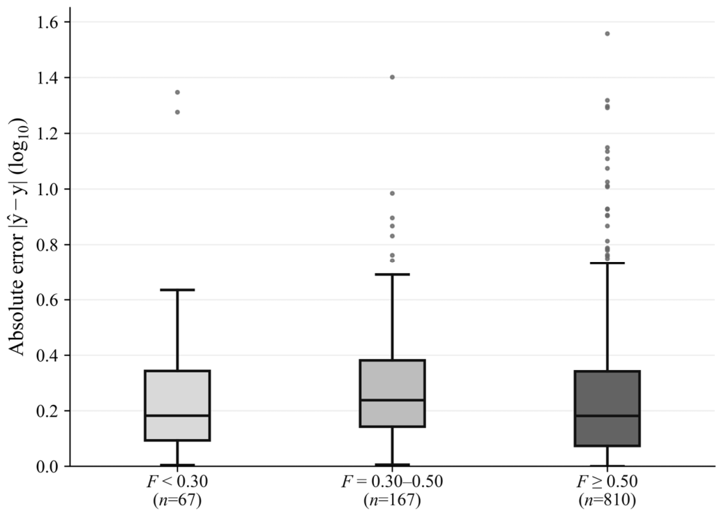
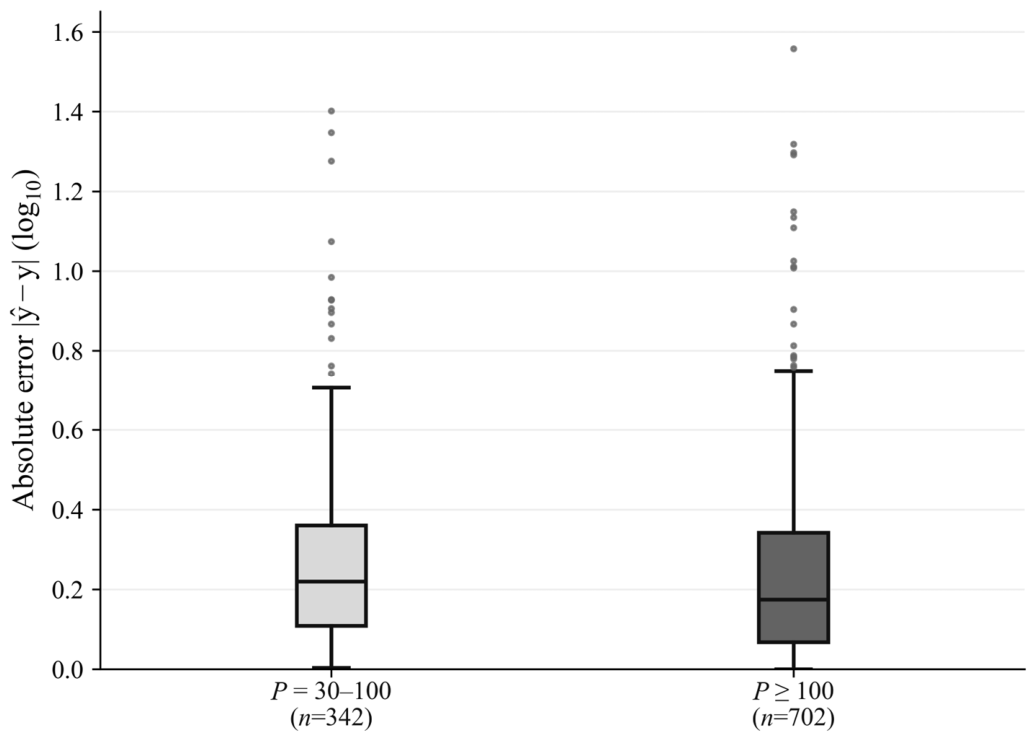
When grouped by F (Figure 7), the RMSE was 0.320 for F ≥ 0.5 (n = 810), but increased to 0.358 for F < 0.5 (n = 234). When grouped by P (Figure 8), the RMSE was 0.319 for P ≥ 100 (n = 702), but increased to 0.348 for P < 100 (n = 342). Further summarized by reliability class, the High samples (P ≥ 100 and F ≥ 0.5) had an RMSE and MAE of 0.321 and 0.235, respectively (n = 687), whereas the Mid samples had an RMSE and MAE of 0.343 and 0.264, respectively (n = 357). These results suggest that the reliability labels constructed from P and F provide diagnostic information on error differences and can support quality-based screening of retrieval results.

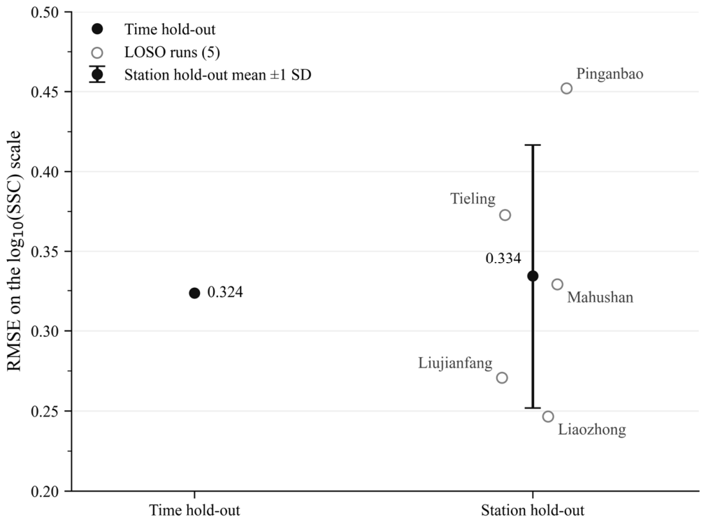
In the extrapolation tests, temporal extrapolation, using earlier years for training and later years for testing, achieved RMSE = 0.324, MAE = 0.250, and R² = 0.444 on the test set (n = 321), which was close to the OOF accuracy of the main experiment (RMSE ≈ 0.329), indicating that the model had a certain degree of robustness to interannual variation. In contrast, leave-one-station-out validation showed clear differences among the held-out stations (

Table 5. Station-specific performance of B_all under leave-one-station-out validation.

Held-Out Station	n	RMSE	MAE	R2	Bias
Tieling	104	0.373	0.277	0.460	0.078
Mahushan	139	0.329	0.252	−0.130	0.203
Pinganbao	282	0.452	0.373	0.203	−0.224
Liaozhong	255	0.246	0.192	0.561	0.042
Liujianfang	264	0.271	0.195	0.490	0.053
Mean		0.334	0.258	0.317	0.030

Notes: All metrics were calculated on the log10(SSC) scale. Bias denotes the mean prediction error (predicted minus observed); positive values indicate overall overestimation, whereas negative values indicate overall underestimation. Mean values are unweighted arithmetic means across the five held-out stations.

). RMSE ranged from 0.246 at Liaozhong to 0.452 at Pinganbao, with an unweighted mean of 0.334, whereas R² ranged from −0.130 at Mahushan to 0.561 at Liaozhong, with an unweighted mean of 0.317. Bias ranged from −0.224 at Pinganbao to 0.203 at Mahushan, indicating station-dependent differences in both error magnitude and direction. Pinganbao exhibited the largest RMSE and the strongest overall underestimation, whereas Mahushan showed a negative R² despite an RMSE close to the five-station mean. Overall, temporal extrapolation remained close to the main OOF result, whereas spatial transferability varied substantially among cross-sections and should be interpreted with site-specific uncertainty (Figure 9).

4. Discussion

4.1. Mechanisms of Coverage Gain and Accuracy Retention in L30–S30 Fusion

The coverage gain produced by L30–S30 fusion was primarily attributable to temporal complementarity in quality-screened observations rather than to an increase in nominal acquisition frequency alone. Inland river observations are frequently affected by clouds, haze, cloud shadows, and insufficient usable water pixels, so one source may remain available on dates when the other is unavailable [29]. Although the HLS framework provides harmonized 30 m L30 and S30 observations on a common spatial grid [17,21], only observations that pass the complete QA, water identification, and P/F screening procedures can be used for SSC retrieval. In this study, same-day dual-source overlap was limited to 0–20 days across the five stations, whereas the date-wise union added 46–96 valid observation days and increased station-month availability to 87.9%. This pattern indicates that the observed coverage gain mainly arose because L30 and S30 supplied usable observations on different dates rather than repeatedly observing the same dates. The High-only sensitivity analysis led to a similar result: after restricting the analysis to records with P ≥ 100 and F ≥ 0.5, the L30–S30 union still increased the number of valid observation days by an average of 73.6% relative to the single sensor with the greater number of valid observation days at each station. Therefore, the improvement in coverage was not mainly driven by the inclusion of marginal-quality observations.

The retention of retrieval accuracy after fusion was likely supported by the combined effects of HLS harmonization, consistent feature construction, and explicit sensor identification. L30 and S30 observations were represented using the same six spectral bands and four derived indices or ratios, all calculated from the median reflectance of valid water pixels within the station ROI. Normalized indices and band ratios emphasize relative spectral contrasts and may partly reduce sensitivity to absolute radiometric differences between sensors [30]. In addition, the binary sensor indicator is_S30 allowed the model to account for residual systematic offsets between L30 and S30 that may remain after harmonization [21]. Consistent with this feature design, B_all showed error levels close to those of the corresponding best single-sensor schemes within both the L30 and S30 subsets. The paired date–block bootstrap tests also showed that the RMSE differences between B_all and the corresponding single-sensor baselines were not statistically significant. These results suggest that the fusion framework increased observation availability without introducing a clear cross-sensor accuracy penalty under the present quality-control and validation settings.

The temporal capability of HLS is often described in terms of the shortened nominal revisit interval achieved by combining Landsat and Sentinel-2 observations [17,21]. For inland river SSC monitoring, however, the more relevant quantity is the number of observations that remain usable after clouds, shadows, water pixel availability, and scene quality are considered. The contribution of this study therefore lies not simply in demonstrating the theoretical temporal advantage of HLS, but in quantifying the increase in quality-screened SSC observation days and evaluating whether this increase is accompanied by a measurable loss of retrieval accuracy. The results indicate that L30–S30 fusion primarily improves monitoring continuity while maintaining an error level comparable to the corresponding single-sensor schemes. This balance between usable temporal coverage and retained accuracy constitutes the main advantage of the fusion strategy for cross-sectional SSC monitoring.

4.2. Sources of Retrieval Uncertainty and Interpretation of Model Performance

The retrieval uncertainty observed in this study likely resulted from the combined effects of aquatic optical complexity, spatial resolution constraints, and variations in usable water pixel conditions. In turbid inland waters, the relationship between SSC and surface reflectance may become nonlinear or gradually saturate as sediment concentration increases, particularly in the visible and near-infrared bands. Other optically active constituents, including colored dissolved organic matter and phytoplankton pigments, may also modify the water-leaving signal and weaken the uniqueness of the spectral response to suspended sediment [12,13]. These effects are particularly relevant for medium-width rivers. The representative water surface widths at the five stations were approximately 90–130 m, so only a limited number of nominal 30 m pixels were available across the river surface. Shoreline mixed pixels, adjacency effects from surrounding land, residual haze, and small geometric mismatches may therefore exert a relatively large influence on the aggregated spectral features [14,15,31]. The fixed water mask, the daily NDWI constraint, median-based spatial aggregation, and P/F screening reduced these effects but could not eliminate them completely. Consistent with this interpretation, the error distributions became wider when the number or proportion of clear-water pixels was low.

Differences in spatial, temporal, and vertical representativeness between satellite observations and in situ SSC records constituted another source of uncertainty. HLS surface reflectance represents the optical condition of the surface or near-surface water layer at the satellite overpass time, whereas the reference variable used in this study was the daily mean SSC for the entire hydrological cross-section. During periods of rapidly changing runoff and sediment transport, particularly around flood events, SSC may vary within the day and across the water column. Consequently, the satellite signal and the daily cross-sectional mean do not necessarily describe exactly the same water–sediment condition. This representativeness difference may partly explain the concentration of predicted values toward the center of the observed range, with some overestimation at low SSC and underestimation at high SSC. Thus, the model is more appropriately interpreted as an empirical estimator of daily mean cross-sectional SSC than as a direct measurement of depth-resolved or instantaneous SSC.

Model form was not the only factor controlling retrieval performance. The additional sensitivity comparison showed that OLS and Ridge produced closely comparable OOF errors, whereas random forest yielded a higher RMSE and a lower R² than Ridge. The tested nonlinear model therefore did not improve the representation of SSC variation under the same samples, predictors, and date-grouped validation framework. This result suggests that the remaining errors cannot be attributed solely to the linear form of Ridge. Instead, they likely reflect the combined influence of optical saturation, mixed pixels, residual atmospheric effects, the limited number of pure-water pixels, station-specific SSC distributions, and the spatial and temporal mismatch between satellite observations and hydrological records. Ridge was consequently retained as the main model because it provided a regularized and interpretable framework for the correlated spectral predictors while achieving an error level comparable to or lower than the alternative models tested in this study.

4.3. Spatial Transferability and Station-Specific Differences

The leave-one-station-out results showed that model transferability varied substantially among the five cross-sections. Pinganbao had the highest RMSE and a negative Bias, indicating greater overall error and a tendency toward underestimation when this station was excluded from model training. This behavior may partly reflect its broader SSC distribution and larger representation of high concentration observations, for which the model showed a stronger tendency to underestimate. In contrast, Mahushan had an RMSE close to the five-station mean but a negative R² and a positive Bias. Because the observed SSC range at Mahushan was relatively narrow, the systematic prediction offset had a greater influence on R², even though its absolute error was not the highest. Liaozhong and Liujianfang showed lower extrapolation errors, indicating that the relationships learned from the other stations were more transferable to these two cross-sections. Overall, the results did not show a simple upstream-to-downstream trend, but instead reflected station-specific differences in SSC distribution and spectral response.

Spatial transferability may also be affected by differences in channel geometry, water depth, flow conditions, bed material, suspended sediment composition, and local hydraulic regulation. These factors can modify both the vertical distribution of SSC and the relationship between surface reflectance and cross-sectional mean SSC, causing a model trained at other stations to perform differently at a new cross-section. Shifosi Reservoir is located between Tieling and Mahushan, and its regulation may influence local flow and sediment conditions within this reach. However, because detailed reservoir-operation and concurrent hydraulic data were not included, the specific contribution of reservoir regulation to the observed station differences could not be isolated. The station extrapolation results therefore indicate that application to new cross-sections should be supported by local validation or recalibration, particularly where hydrodynamic and sediment conditions differ from those represented in the training data.

4.4. Practical Implications and Applicability Boundaries

The main practical value of L30–S30 fusion lies in improving the temporal continuity of quality-screened SSC observations rather than in producing a marked increase in retrieval accuracy. The additional valid observation dates can provide more complete support for identifying seasonal variation, flood season responses, and interannual changes in river sediment conditions. The reliability labels further allow the retrieval results to be used according to their quality. High-reliability records can be prioritized for spatial mapping, temporal comparison, and trend analysis, whereas Mid-reliability records may be retained to improve time-series completeness but should be accompanied by explicit quality flags and interpreted cautiously in quantitative analyses. In this way, the fusion and reliability classification framework provides a practical balance between observation coverage and confidence in the retrieval results.

The retrieval results should nevertheless be used within the scope supported by the data and validation design. The model estimates daily mean cross-sectional SSC under ice-free conditions and is not intended to replace routine hydrological station measurements, resolve the vertical distribution of SSC, or provide instantaneous sediment fluxes for high-precision engineering calculations. Its direct application is most appropriate for quality-screened monitoring, relative comparison, and supplementary analysis in river reaches with conditions similar to those represented by the five training stations. For new rivers or cross-sections with different channel geometry, hydrodynamic conditions, sediment composition, or optical properties, independent validation and, where necessary, local recalibration should be conducted before operational use.

4.5. Limitations and Future Work

This study has several limitations. First, model development and validation were based on five hydrological stations located along the middle and lower reaches of the Liaohe mainstream. Although date-grouped cross-validation, temporal extrapolation, and leave-one-station-out validation were used, the applicability of the model to other rivers, tributaries, reservoirs, backwater zones, and reaches with substantially different channel or sediment conditions has not yet been independently verified. Additional stations and multi-river datasets are therefore needed to further evaluate spatial transferability beyond the present study area.

Second, the reference variable was the daily mean SSC for the entire hydrological cross-section, whereas HLS surface reflectance represents the surface or near-surface optical condition at the satellite overpass time. Observation-specific measurement uncertainty and complete concurrent hydraulic variables were not incorporated into the present analysis. Consequently, the separate effects of sampling uncertainty, within-day SSC variation, flow conditions, and vertical sediment distribution could not be quantified directly. In addition, winter observations from December to February were excluded because of snow, ice, and low solar elevation. The conclusions therefore apply mainly to ice-free and open-water conditions and should not be extended directly to year-round SSC monitoring or annual sediment load estimation.

Third, the fixed water mask and the 800 m radius ROI improved consistency among dates and stations, but they may not fully represent short-term changes in water extent caused by floodplain inundation, channel migration, or pronounced seasonal water-level variation. Under these conditions, the number and spatial distribution of pure-water and mixed pixels may change even when the same statistical window is used. Future studies could evaluate dynamic water masks and spatial windows that adapt to river stage or water extent.

Finally, Ridge regression provided a regularized and interpretable framework for the correlated spectral predictors and achieved performance comparable to or better than the alternative models tested in this study. However, the present model comparison does not exclude possible improvements with other algorithms or more informative predictors. Future work should incorporate additional hydrological and sediment variables, physically meaningful spectral features, independent station data, and dynamic spatial constraints to improve retrieval reliability and transferability under more diverse river conditions.

5. Conclusions

Based on daily mean cross-sectional SSC records from five hydrological stations and L30/S30 surface reflectance data during the ice-free months of 2016–2022, this study evaluated single-sensor and fusion retrieval schemes under date-grouped cross-validation, temporal extrapolation, and leave-one-station-out validation. The fusion scheme B_all achieved an OOF RMSE of 0.329, MAE of 0.245, R² of 0.454, and a Bias of 0.002 on the log10(SSC) scale. The model captured the general variation in cross-sectional SSC with limited overall systematic bias, although prediction errors were more evident at the lower and higher ends of the observed SSC range.

L30–S30 fusion substantially increased the temporal availability of quality-screened observations without clear evidence of accuracy degradation relative to the corresponding single-sensor schemes. Compared with the single sensor with the greater number of valid observation days at each station, the date-wise union increased valid observation days by an average of 64.6%, while station-month availability reached 87.9%. Reliability labels based on clear-water pixel number and proportion further distinguished observations with different error levels. High-reliability records are more suitable for mapping, temporal comparison, and trend analysis, whereas Mid-reliability records may supplement time series but should be accompanied by explicit quality information and interpreted cautiously in quantitative analyses.

Temporal extrapolation produced an error level close to that of the main cross-validation result, whereas spatial transferability varied substantially among stations. The proposed workflow is therefore most appropriate as an empirical approach for quality-screened estimation of daily mean cross-sectional SSC under ice-free conditions in river reaches similar to those represented by the training data. Applications to new rivers or cross-sections should be supported by independent validation and, where necessary, local recalibration.

References

1. Roushangar, K.; Alirezazadeh Sadaghiani, A.; Nourani, V. Comparative trend analysis of suspended sediment concentration and streamflow: A multi-method framework. Water Resour. Manag. 2025, 39, 5991–6007. [Google Scholar] [CrossRef]
2. Li, K.; Liu, D.; Qiu, Z.; Duan, M.; Wei, X.; Duan, H. Human management decreased suspended particle size in the Loess Plateau rivers during the 1980s to the 2010s. Sustainability 2024, 16, 799. [Google Scholar] [CrossRef]
3. Moridnejad, A.; Abdollahi, H.; Alavipanah, S.K.; Samani, J.M.V.; Moridnejad, O.; Karimi, N. Applying artificial neural networks to estimate suspended sediment concentrations along the southern coast of the Caspian Sea using MODIS images. Arab. J. Geosci. 2015, 8, 891–901. [Google Scholar] [CrossRef]
4. Xiao, Y.; Yang, F.S.; Su, L.; Li, J.W. Fluvial sedimentation of the permanent backwater zone in the Three Gorges Reservoir, China. Lake Reserv. Manag. 2015, 31, 324–338. [Google Scholar] [CrossRef]
5. Frogner-Kockum, P.; Göransson, G.; Haeger-Eugensson, M. Impact of climate change on metal and suspended sediment concentrations in urban waters. Front. Environ. Sci. 2020, 8, 588335. [Google Scholar] [CrossRef]
6. Wackerman, C.; Hayden, A.; Jonik, J. Deriving spatial and temporal context for point measurements of suspended-sediment concentration using remote-sensing imagery in the Mekong Delta. Cont. Shelf Res. 2017, 147, 231–245. [Google Scholar] [CrossRef]
7. Jeon, J.-H.; Park, C.-G.; Choi, D.; Kim, T. Characteristics of suspended sediment loadings under Asian summer monsoon climate using the Hydrological Simulation Program-FORTRAN. Sustainability 2017, 9, 44. [Google Scholar] [CrossRef]
8. Wang, J.; Yan, Y.; Bai, J.; Su, X. Influences of riverbed siltation on redox zonation during bank filtration: A case study of Liao River, Northeast China. Hydrol. Res. 2020, 51, 1478–1489. [Google Scholar] [CrossRef]
9. Reisinger, A.; Gibeaut, J.C.; Tissot, P.E. Estuarine suspended sediment dynamics: Observations derived from over a decade of satellite data. Front. Mar. Sci. 2017, 4, 233. [Google Scholar] [CrossRef]
10. Han, B.; Loisel, H.; Vantrepotte, V.; Mériaux, X.; Bryère, P.; Ouillon, S.; Dessailly, D.; Xing, Q.; Zhu, J. Development of a semi-analytical algorithm for the retrieval of suspended particulate matter from remote sensing over clear to very turbid waters. Remote Sens. 2016, 8, 211. [Google Scholar] [CrossRef]
11. Robert, E.; Grippa, M.; Kergoat, L.; Pinet, S.; Gal, L.; Cochonneau, G.; Martinez, J.-M. Monitoring water turbidity and surface suspended sediment concentration of the Bagre Reservoir (Burkina Faso) using MODIS and field reflectance data. Int. J. Appl. Earth Obs. Geoinf. 2016, 52, 243–251. [Google Scholar] [CrossRef]
12. Ansper-Toomsalu, A.; Uusõue, M.; Kangro, K.; Hieronymi, M.; Alikas, K. Suitability of different in-water algorithms for eutrophic and absorbing waters applied to Sentinel-2 MSI and Sentinel-3 OLCI data. Front. Remote Sens. 2024, 5, 1423332. [Google Scholar] [CrossRef]
13. Wu, Z.; Pang, J.; Li, J.; Wang, Y.; Ruan, J.; Zhang, X.; Yang, L.; Pang, Y.; Gao, Y. A review of remote sensing-based water quality monitoring in turbid coastal waters. Intell. Mar. Technol. Syst. 2025, 3, 24. [Google Scholar] [CrossRef]
14. Frasson, R.P.M.; Ardila, D.R.; Pease, J.; Hestir, E.; Bright, C.; Carter, N.; Dekker, A.G.; Thompson, D.R.; Green, R.O.; Held, A. The impact of spatial resolution on inland water quality monitoring from space. Environ. Res. Commun. 2024, 6, 101003. [Google Scholar] [CrossRef]
15. Huangfu, K.; Li, J.; Zhang, X.; Zhang, J.; Cui, H.; Sun, Q. Remote estimation of water quality parameters of medium- and small-sized inland rivers using Sentinel-2 imagery. Water 2020, 12, 3124. [Google Scholar] [CrossRef]
16. Ping, B.; Meng, Y.; Su, F. An enhanced linear spatio-temporal fusion method for blending Landsat and MODIS data to synthesize Landsat-like imagery. Remote Sens. 2018, 10, 881. [Google Scholar] [CrossRef]
17. Claverie, M.; Ju, J.; Masek, J.G.; Dungan, J.L.; Vermote, E.F.; Roger, J.-C.; Skakun, S.V.; Justice, C. The Harmonized Landsat and Sentinel-2 surface reflectance data set. Remote Sens. Environ. 2018, 219, 145–161. [Google Scholar] [CrossRef]
18. Chen, X.; Jiang, J.; Li, H. Drought and flood monitoring of the Liao River Basin in Northeast China using extended GRACE data. Remote Sens. 2018, 10, 1168. [Google Scholar] [CrossRef]
19. Chen, Y.; Wang, L.-L.; Fan, H.-M. Sedimentation analysis in middle and lower reaches of Liaohe River. Water Resour. 2020, 47, 87–94. [Google Scholar] [CrossRef]
20. Bailey, S.W.; Werdell, P.J. A multi-sensor approach for the on-orbit validation of ocean color satellite data products. Remote Sens. Environ. 2006, 102, 12–23. [Google Scholar] [CrossRef]
21. Ju, J.; Zhou, Q.; Freitag, B.; Roy, D.P.; Zhang, H.K.; Sridhar, M.; Mandel, J.; Arab, S.; Schmidt, G.; Crawford, C.J.; et al. The Harmonized Landsat and Sentinel-2 version 2.0 surface reflectance dataset. Remote Sens. Environ. 2025, 324, 114723. [Google Scholar] [CrossRef]
22. Zhu, Z.; Wang, S.; Woodcock, C.E. Improvement and expansion of the Fmask algorithm: Cloud, cloud shadow, and snow detection for Landsats 4–7, 8, and Sentinel 2 images. Remote Sens. Environ. 2015, 159, 269–277. [Google Scholar] [CrossRef]
23. McFeeters, S.K. The use of the Normalized Difference Water Index (NDWI) in the delineation of open water features. Int. J. Remote Sens. 1996, 17, 1425–1432. [Google Scholar] [CrossRef]
24. Lacaux, J.P.; Tourre, Y.M.; Vignolles, C.; Ndione, J.A.; Lafaye, M. Classification of ponds from high-spatial resolution remote sensing: Application to Rift Valley Fever epidemics in Senegal. Remote Sens. Environ. 2007, 106, 66–74. [Google Scholar] [CrossRef]
25. Tucker, C.J. Red and photographic infrared linear combinations for monitoring vegetation. Remote Sens. Environ. 1979, 8, 127–150. [Google Scholar] [CrossRef]
26. Duan, M.; Qiu, Z.; Li, R.; Li, K.; Yu, S.; Liu, D. Monitoring suspended sediment transport in the Lower Yellow River using Landsat observations. Remote Sens. 2024, 16, 229. [Google Scholar] [CrossRef]
27. Hoerl, A.E.; Kennard, R.W. Ridge regression: Biased estimation for nonorthogonal problems. Technometrics 1970, 12, 55–67. [Google Scholar] [CrossRef]
28. Ritter, A.; Muñoz-Carpena, R. Performance evaluation of hydrological models: Statistical significance for reducing subjectivity in goodness-of-fit assessments. J. Hydrol. 2013, 480, 33–45. [Google Scholar] [CrossRef]
29. Ju, J.; Roy, D.P. The availability of cloud-free Landsat ETM+ data over the conterminous United States and globally. Remote Sens. Environ. 2008, 112, 1196–1211. [Google Scholar] [CrossRef]
30. Cao, S.; Danielson, B.; Clare, S.; Koenig, S.; Campos-Vargas, C.; Sanchez-Azofeifa, A. Radiometric calibration assessments for UAS-borne multispectral cameras: Laboratory and field protocols. ISPRS J. Photogramm. Remote Sens. 2019, 149, 132–145. [Google Scholar] [CrossRef]
31. Palmer, S.C.J.; Kutser, T.; Hunter, P.D. Remote sensing of inland waters: Challenges, progress and future directions. Remote Sens. Environ. 2015, 157, 1–8. [Google Scholar] [CrossRef]
Figure 1. The location of the study area and hydrological stations in the middle and lower reaches of the Liaohe River, China. The blue line denotes the Liaohe River, red circles denote the five hydrological stations used for SSC sampling and validation, and the inset shows the location of Liaoning Province in China.
Water 18 01830 g001
Figure 2. Comparison of root mean square error (RMSE) among the three modeling schemes across different subsets (log10 scale).
Water 18 01830 g002
Figure 3. ΔRMSE and its 95% confidence intervals under fair subset comparisons. ΔRMSE is defined as RMSE(baseline) − RMSE(B_all). A1 was used as the baseline for the L30 subset, and A2 was used as the baseline for the S30 subset. Points indicate the estimated ΔRMSE values, horizontal lines indicate the 95% confidence intervals, and the dashed line denotes 0. Confidence intervals crossing 0 indicate that the RMSE difference between the fusion scheme and the corresponding single-sensor model in that subset is not statistically significant.
Water 18 01830 g003
Figure 4. Observed-versus-predicted scatter plots of the three modeling schemes for all samples (out-of-fold (OOF) predictions). Panel (a) shows A1 (L30-only), panel (b) shows A2 (S30-only), and panel (c) shows B_all (Fusion).
Water 18 01830 g004
Figure 5. Valid observation days at each station and the complementary contributions of HLS L30 (Landsat 8/9) and HLS S30 (Sentinel-2).
Water 18 01830 g005
Figure 6. Comparison of time series of valid observation days at the monthly scale. This figure shows the monthly sums of valid observation days across the five stations and is used to characterize the variation in overall observation density at the monthly scale.
Water 18 01830 g006
Figure 7. Relationship between clear-water pixel proportion (F) and absolute error.
Water 18 01830 g007
Figure 8. Relationship between number of clear-water pixels (P) and absolute error.
Water 18 01830 g008
Figure 9. Root mean square error (RMSE) of B_all under temporal extrapolation and leave-one-station-out validation. Station labels identify the corresponding held-out test stations, and the horizontal offsets of the individual station points are used only for visual separation.
Water 18 01830 g009