Development and Application of a River–Sewer Water Level Correlation Model for Identifying Inflow and Infiltration Diagnosis: A Case Study of Zhongshan’s Regional Sewage Network

Abstract

Identifying inflow and infiltration (I/I) in urban sewer networks is challenging due to nonlinear hydraulic interactions and time-lag effects between river stages and pipeline water levels. This study proposes a multi-scale fusion correlation model integrating Dynamic Time Warping (DTW), Pearson correlation, and Spearman rank correlation coefficients. The framework evaluates water level sequences across temporal windows (2, 6, and 12 h) under flexible displacement constraints (1 and 2 h), utilizing a dynamic weight-allocation mechanism based on sequence volatility and data density. Leveraging a 12-month monitoring dataset from 513 sensing devices in Zhongshan City, China, the model was evaluated on 36 typical water-level sequences. It achieved a classification accuracy of 91.7% for low-correlation sequences and perfect accuracy (100%) for both medium- and high-correlation levels. Furthermore, practical deployment in the Shaxi–Qijiang Highway section and Yicheng Area successfully isolated multiple vulnerable pipe segments suffering from Baishiyong River (tidal) water intrusion, yielding an empirical field-verification hit rate of 83.3%. The results demonstrate that the proposed framework effectively overcomes temporal asynchrony and nonlinear hydraulic noise, providing a robust, data-driven diagnostic tool for urban drainage infrastructures.

1. Introduction

As urban water environment governance enters the stage of fine-grained management and control [1], the problem of extraneous water intrusion—defined herein as water entering the sewer system from non-domestic sources, primarily including river inflow from the Baishiyong River (a tide-influenced tributary of the Qijiang River in Zhongshan City, e.g., tidal backflow) and groundwater infiltration through pipe defects (collectively known as inflow and infiltration, I/I)—has become a critical bottleneck restricting the improvement of influent concentration and the optimization of operational efficiency in wastewater treatment plants (WWTPs) [2,3,4]. Aligned with national and provincial quality-efficiency enhancement directives [5], the Zhongshan Water Affairs Bureau has explicitly proposed a “quality and efficiency enhancement” goal to ensure that the Biochemical Oxygen Demand (BOD) concentration of WWTP influent exceeds 100 mg/L. Among the contributing factors, river water I/I and groundwater infiltration are the core causes of low pollutant concentrations in the influent [6,7,8]. Currently, the identification and source-tracing of I/I in drainage networks still primarily rely on manual CCTV inspections, smoke testing, or localized flow balancing [9,10]. These traditional diagnostic methods are characterized by low efficiency, high operational costs, and limited spatial–temporal continuity, making it difficult to meet the urgent demands for proactive, intelligent operation and maintenance (O&M) in large-scale, complex drainage catchments [11].

To overcome these diagnostic constraints, various emerging tracking modalities and data-driven paradigms have been developed globally to trace inflow and infiltration (I/I) dynamics. These primarily encompass thermal tracer methods utilizing distributed temperature sensing (DTS) to isolate groundwater leakage paths, hydrochemical isotope mixing models aimed at quantifying dilution components, and high-resolution hydraulic monitoring coupled with data-driven anomaly detection models. While these advanced tracking configurations significantly bolster regional source-tracing precision, their vast instrumentation expenses, complex chemical sampling protocols, and vulnerability to sensor drift or signal dropouts heavily curtail their pervasive, large-scale field scalability in complex municipal catchments.

In recent years, the wide deployment of smart water sensors has accumulated a vast number of high-frequency, continuous monitoring streams regarding both river stages and sewer network water levels, providing a promising data-driven paradigm for identifying I/I intrusion [12,13]. However, in real-world urban hydrodynamics, river level fluctuations and the corresponding hydraulic responses in adjacent sewer pipes do not occur synchronously. Constrained by pipeline friction, backwater effects, and pump station gate regulations, there generally exists a significant, time-varying time-lag effect alongside highly nonlinear mapping relationships between the two boundary conditions [14]. Conventional synchronization-based correlation methods, such as the classical Pearson correlation coefficient, inherently assume zero phase-shift and linear interactions. Consequently, they struggle to capture the transient water-wave propagation and phase offsets, leading to substantial false negatives or misclassifications when delineating zones vulnerable to river intrusion [15].

To address the aforementioned technical bottlenecks, the DTW algorithm can effectively resolve the asynchronous phase difference in time series through its nonlinear warping path alignment strategy [16,17]. Meanwhile, the Pearson correlation coefficient provides a precise measure of the linear synergy between variables [18,19,20], whereas the Spearman rank correlation coefficient offers excellent robustness against outliers and effectively captures the monotonic trends between variables [21,22]. Consequently, these three methods exhibit significant complementary advantages in the dimension of feature representation [23].

To leverage these strengths, this study establishes a novel multi-scale fusion correlation model that couples DTW distance, Pearson, and Spearman coefficients to accurately identify river water intrusion. The major scientific contributions and specific objectives of this work are threefold:

(1)

An adaptive data-preprocessing module is embedded to dynamically strip out sensor outliers using change-rate thresholds.

(2)

A multi-scale temporal windowing scheme (2 h, 6 h, and 12 h) under flexible lag constraints (1 h and 2 h) is integrated with a volatility-driven dynamic weight allocation mechanism to faithfully capture transient hydraulic coupling.

(3)

The proposed framework is validated using a project-verified database from 513 devices across Zhongshan City, China, achieving an 83.3% empirical field hit rate. This research delivers an efficient, robust digital tool for localized I/I diagnosis and quality enhancement of urban drainage infrastructures.

Compared to existing paradigms in the literature, the novelty of this fusion framework lies in its ability to overcome specific limitations of single-method approaches. Traditional synchronous correlation methods (e.g., Pearson) fail to capture the 1–2 h hydraulic lags prevalent in tidal networks. While standalone DTW addresses asynchrony, it lacks the complementary feature extraction provided by our multi-metric fusion. Unlike physics-based hydraulic models (e.g., SWMM) that require extensive site-specific calibration, our data-driven approach supports near-real-time analysis without parameter tuning. Furthermore, compared to emerging machine learning models (e.g., LSTM or Siamese networks), our framework does not require hundreds of labeled training samples—a critical advantage given the scarcity of verified I/I field data—and retains full physical interpretability for O&M engineers.

2. Materials and Methods

2.1. Study Area Description

This study selects the central urban area and Shaxi Town of Zhongshan City, located in Guangdong Province, China, as the macro research region. This area features a subtropical monsoon climate with high-density urban catchments and intricate tidal river systems. The total length of the drainage network in this area is approximately 2800 km, with a total of 513 sets of online water-level monitoring devices deployed. The 513 pressure-type water level sensors (±1 mm accuracy, IP68 rated) installed in manholes were sampled at 10 min intervals, complementing river level data from the Baishiyong Drainage Pumping Station. Considering the topological characteristics of the pipe network and the actual conditions of I/I intrusion, two representative, hydraulically vulnerable pilot sub-zones were isolated for precision engineering deployment: the Shaxi–Qijiang Road section (comprising 6 monitoring points, characterized by heavy commercial blocks and frequent tidal river I/I) and the Yicheng area (comprising 5 monitoring points, characterized by industrial–residential mixed usage and high groundwater infiltration risk). The river involved in the correlation analysis of this study is the Baishiyong River, a tide-influenced tributary of the Qijiang River traversing the study area. It should be distinguished from three other local rivers within Shaxi Town (i.e., the Shijiao, Chizhou, and Shaxi Rivers), which are not directly analyzed here. River water level monitoring data were uniformly sourced from the Baishiyong Drainage Pumping Station. The sampling frequency for all monitoring data is 10 min, covering a time span from January to December 2024.

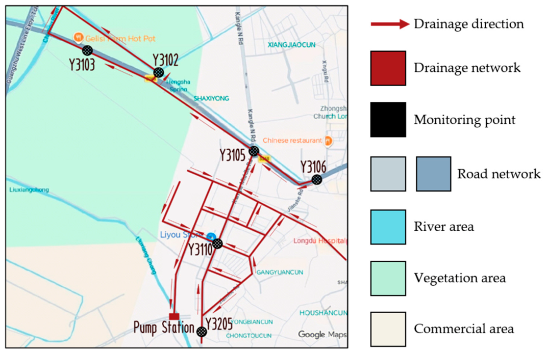
The subsequent paragraphs detail the basic characteristics of the two pilot sub-zones selected for this study. The Shaxi Town jurisdiction covers an area of 55 km², managing a population of nearly 400,000. The total annual water consumption is approximately 30 million tons, with an average daily sewage discharge of about 80,000 tons. The region possesses a well-developed water system, with primary rivers including the Shijiao River, Chizhou River, and Shaxi River. The Qijiang Highway sewage catchment is a subordinate part of the Shaxi Town sewage system. Due to the combined drainage system and high population density, sewage concentrations in this area have remained consistently low, indicating a severe problem with I/I intrusion [24]. Sewage within this section is collected via Kangle Middle Road, discharged into the Qijiang Highway main pipe, and eventually flows into the Shaxi–Yunhan Pumping Station. The spatial distribution of sewage mains and monitoring points in the Shaxi–Qijiang Highway section is illustrated in Figure 1. Detailed attributes of the six monitoring sensors in this sub-zone are listed in

Table 1. Core attributes and standardized UTM coordinates (Zone 50 N, WGS84) of the monitoring water-level sensors in the Shaxi–Qijiang Road section.

Monitoring Point ID	Monitoring Point Name	UTM Coordinates (Zone 49 N, WGS84)
Y3103	Qijiang Highway Sewage Main (South) Level Gauge	49 N 734,868.18 E 2,492,747.15 N
Y3102	Qijiang Highway Sewage Main (North) Level Gauge	49 N 735,353.55 E 2,492,598.01 N
Y3105	Qijiang Highway Sewage Main (Downstream) Level Gauge	49 N 736,116.30 E 2,491,997.46 N
Y3106	Qijiang Highway Sewage Main (Upstream) Level Gauge	49 N 736,490.34 E 2,491,753.21 N
Y3110	Kangle Middle Road (North Side) Sewage Main Level Gauge	49 N 735,845.99 E 2,491,290.68 N
Y3205	Kangle Middle Road (South Side) Sewage Main Level Gauge	49 N 735,742.69 E 2,490,556.84 N

.

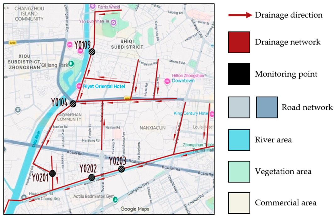
In what follows, the basic characteristics of the Yicheng pilot sub-zone are described, which is located within the old urban district of Zhongshan City. This district is characterized by densely populated residential blocks, aging combined sewer systems, and a history of urban waterlogging issues, making it a representative case study for I/I investigation. The Yicheng catchment covers a pollution collection area of approximately 8 km², primarily serving the old urban district. Although no open river channels pass through the area, there are 16 covered culverts with a total length of about 12.32 km. Sewage is discharged into these covered culverts via combined pipes and is subsequently directed to the Zhongjia Sewage Treatment Plant through interceptors or pumping stations. The spatial distribution of sewage mains and monitoring points in the Yicheng Area is illustrated in Figure 2. Detailed attributes of the five monitoring sensors in this sub-zone are listed in

Table 2. Core attributes and standardized UTM coordinates (Zone 50 N, WGS84) of the monitoring water-level sensors in the Yicheng area.

Monitoring Point ID	Monitoring Point Name	UTM Coordinates (Zone 49 N, WGS84)
Y0109	Nanji Road Sewage Main Level Gauge	49 N 742,920.17 E 2,492,708.64 N
Y0104	Huaguang Road Sewage Main Level Gauge	49 N 742,482.31 E 2,491,799.80 N
Y0201	Yuekai Road Sewage Main Level Gauge	49 N 742,289.83 E 2,490,756.50 N
Y0202	Baishi Road Sewage Main Level Gauge	49 N 742,946.36 E 2,490,711.23 N
Y0203	Bo’ai 3rd Road (West Side) Sewage Main Level Gauge	49 N 743,396.10 E 2,490,841.64 N

.

2.2. Data Preprocessing Workflow

To ensure data quality and analytical reliability, a standardized preprocessing workflow was implemented on the raw monitoring sequences. First, anomalous data segments with a continuous missing ratio exceeding 5% were excluded. Given that the excluded segments accounted for less than 2% of the total monitoring duration and were primarily concentrated in non-rainy periods, their removal did not affect the integrity of the analysis of key hydrological events. Second, linear interpolation was employed to supplement short-term missing values [25]. Subsequently, the interquartile range (IQR) method and Z-score method were jointly applied for outlier detection and correction [26]. In particular, an adaptive rate-of-change threshold (>0.5 m/unit time) derived from local hydraulic capacities was embedded to dynamically strip out instrument-induced spikes. Finally, a moving average method was utilized for sequence smoothing and noise reduction to ensure the data met the precision requirements for subsequent model analysis [27].

2.3. Principles of the DTW Algorithm

DTW is an elastic distance measure that aligns two time series by nonlinearly warping their time axes. Given two water-level time series, denoted as

$$\mathrm{X}=\left(x_1,x_2,\dots ,x_N\right) \mathrm{and} \mathrm{Y}=\left(y_1,y_2,\dots ,y_M\right),$$

DTW seeks an optimal alignment path that minimizes the cumulative distance between them while strictly preserving the temporal order of observations. This capability effectively accommodates time-axis scaling, phase shifts, and time-lag effects, rendering it particularly suitable for correlation analysis in scenarios where river water levels and pipe network responses exhibit asynchronous hydraulic behavior.

The core mechanism of DTW proceeds as follows: First, an $N\times M$ local distance matrix $\mathrm{C}$ is constructed, with each element

$$c\left(i,j\right)=d\left(x_i,y_j\right),$$

where $d(x_i,y_j)$ is typically chosen as the squared Euclidean distance, $d(x_i,y_j)=(x_i-y_j{)}^2$. Next, a dynamic programming approach computes the accumulated cost matrix $\mathrm{D}$, where $D(i,j)$ represents the minimum cumulative distance to align the prefix $\mathrm{X}[1:i]$ with $\mathrm{Y}[1:j]$. The recurrence relation is

$$D\left(i,j\right)=c\left(i,j\right)+\min \left\{D\left(i-1,j\right),\mathrm{ }D\left(i,j-1\right),\mathrm{ }D\left(i-1,j-1\right)\right\},$$

with boundary conditions

$$D\left(\mathrm{0,0}\right)=0, D\left(i,0\right)=\mathrm{\infty }\mathrm{ }\left(i>0\right),D\left(0,j\right)=\mathrm{\infty }\mathrm{ }\left(j>0\right).$$

The three transition options correspond, respectively, to expansion (aligning one point of $\mathrm{Y}$ with multiple points of $\mathrm{X}$), contraction (the reverse), and direct match (one-to-one alignment). Upon completion of the DP fill, the final DTW distance is given by $D(N,M)$. The optimal warping path can be retrieved by backtracking from $(N,M)$ to $\left(\mathrm{1,1}\right)$, at each step selecting the predecessor cell that yielded the minimum value in the recurrence. This path defines the pairwise correspondence between data points, and the resulting cumulative distance serves as a quantitative measure of morphological similarity between the two sequences [28].

Despite its effectiveness, the classical DTW algorithm has two notable limitations: (i) high computational complexity of $O(N\cdot M)$, which becomes prohibitive for long sequences, and (ii) sensitivity to boundary conditions, since it forces the first and last points to be aligned even when they are not temporally corresponding in practice. To mitigate these issues, we adopt the Sakoe–Chiba band constraint [29], which restricts the admissible warping path to a narrow corridor around the diagonal, defined by

$$\mid i-j\mid \le w,$$

where $w$ is the maximum allowed displacement (in index units). Based on the actual hydraulic lag characteristics observed in the study area, we set $w$ to correspond to a time shift of 1–2 h. This constraint not only prevents pathological warping (e.g., extreme stretching or compression) but also reduces the time complexity to $O(N\cdot w)$, thereby significantly improving computational efficiency while maintaining sufficient analytical accuracy for the intended correlation analysis [30].

2.4. Principles of the Pearson Correlation Coefficient

The Pearson correlation coefficient is used to measure the intensity of the linear correlation between two continuous variables, with its value ranging from [−1, 1]. An absolute value approaching 1 indicates a strong linear correlation, while a value approaching 0 indicates the absence of a significant linear relationship. It is defined as the ratio of the covariance of two variables to the product of their respective standard deviations. The formula for the population correlation coefficient is as follows:

$${\rho }_{X,Y}={\displaystyle \frac{\mathrm{cov}\left(X,Y\right)}{{\sigma }_X{\sigma }_Y}}={\displaystyle \frac{E\left[\left(X-{\mu }_X\right)\left(Y-{\mu }_Y\right)\right]}{{\sigma }_X{\sigma }_Y}}$$

(1)

In this formula, ${\mu }_X \mathrm{a}\mathrm{n}\mathrm{d} {\mu }_Y$ represent the population means of variables X and Y, respectively, while ${\sigma }_X \mathrm{a}\mathrm{n}\mathrm{d} {\sigma }_Y$ represent the population standard deviations of variables X and Y, respectively.

The Pearson correlation coefficient estimated based on sample data is commonly denoted as r, and the calculation formula is as follows:

$$r={\displaystyle \frac{{\displaystyle {\sum }_{i=1}^n} \left(X_i-\overline{X}\right)\left(Y_i-\overline{Y}\right)}{\sqrt{{\displaystyle {\sum }_{i=1}^n} (X_i-\overline{X}{)}^2}\sqrt{{\displaystyle {\sum }_{i=1}^n} (Y_i-\overline{Y}{)}^2}}}$$

(2)

Meanwhile, r can also be estimated using the mean of the standard scores of the sample points, with the equivalent expression as follows:

$$r={\displaystyle \frac{1}{n-1}}{\displaystyle \sum _{i=1}^n} \left({\displaystyle \frac{X_i-\overline{X}}{{\sigma }_X}}\right)\left({\displaystyle \frac{Y_i-\overline{Y}}{{\sigma }_Y}}\right)$$

(3)

In the above formula, $\overline{X}$ and $\overline{Y}$ are the sample means, ${\sigma }_X \mathrm{a}\mathrm{n}\mathrm{d} {\sigma }_Y$ are the sample standard deviations, and n is the sample size.

The Pearson correlation coefficient is characterized by its computational simplicity and clear physical significance; however, it is applicable only to the measurement of linear relationships and is relatively sensitive to outliers. In this study, it is primarily employed to evaluate the linear synergy of the fluctuation amplitudes between river and pipe network water levels [31].

2.5. Principles of the Spearman Rank Correlation Coefficient

The Spearman rank correlation coefficient is calculated based on the rank order of variables and is used to evaluate the monotonic trend between two variables, with a value range also spanning [−1, 1]. This coefficient does not depend on the assumption of a normal distribution and exhibits strong robustness against outliers. For a sequence with a sample size of n, the raw data are converted into rank data, and the correlation coefficient ρ is as follows:

$$\rho ={\displaystyle \frac{\sum _i \left(x_i-\overline{x}\right)\left(y_i-\overline{y}\right)}{\sqrt{\sum _i (x_i-\overline{x}{)}^2\sum _i (y_i-\overline{y}{)}^2}}}$$

(4)

This coefficient can effectively capture the monotonic nonlinear relationships between variables, compensating for the limitations of the Pearson correlation coefficient in nonlinear scenarios. By complementing the Pearson coefficient, it helps to comprehensively reflect the trend consistency of water-level time series [32].

2.6. Integrated Algorithm Design

This study constructs a river–pipe network water level correlation analysis model based on a three-level fusion architecture, achieving a multi-feature, multi-scale, and dynamic evaluation of correlation [33]. The specific design is as follows:

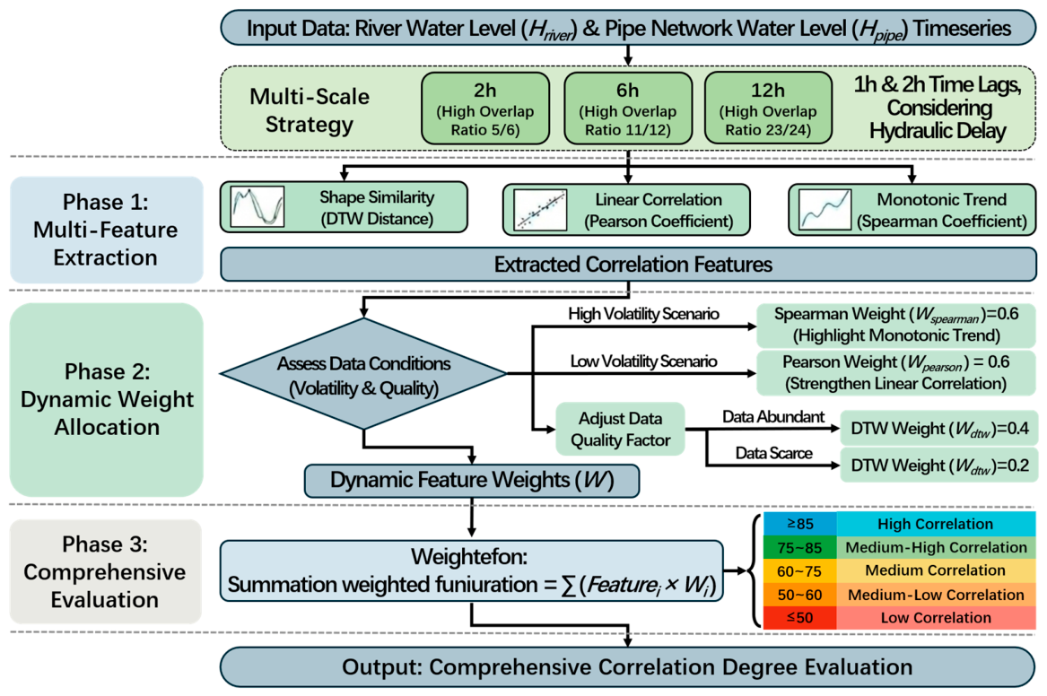
(1) Feature Extraction: Calculate the DTW distance (characterizing morphological similarity), the Pearson correlation coefficient (characterizing linear correlation), and the Spearman rank correlation coefficient (characterizing monotonic trends) to extract the core association features of the water-level sequences. To clarify the functional distinctions, applicability boundaries, and complementary roles of the three models in our fusion framework, we summarize their core characteristics in

Table 3. Comparative characteristics of DTW, Pearson correlation coefficient, and Spearman rank correlation coefficient and their respective roles in the proposed fusion model.

Model	Core Function	Time-Lag Handling	Linearity Assumption	Outlier Robustness	Primary Role
DTW	Morphological similarity	Yes	No	Medium	Resolve temporal asynchrony between river and sewer responses
Pearson	Linear correlation	No	Yes	Low	Quantify linear amplitude synergy of water-level fluctuations
Spearman	Monotonic trend	No	No	High	Capture consistent trend alignment while suppressing noise interference

.

Distinct from existing single-metric approaches in the literature, the integration of these three complementary algorithms addresses the critical gap in handling asynchronous, nonlinear hydraulic interactions prevalent in tidal sewer networks.

The selection of DTW, Pearson correlation coefficient, and Spearman rank correlation coefficient is grounded in the unique hydraulic characteristics of tidal drainage networks and practical deployment constraints, as summarized in Table 2. Tidal systems induce consistent 1–2 h hydraulic lags between river stages and sewer responses, which synchronous methods cannot resolve; DTW addresses this via nonlinear time-axis warping, while Pearson and Spearman capture complementary linear and monotonic trend features. Field data also suffer from sensor noise and missing values, necessitating a balance between sensitivity and robustness: Pearson quantifies linear synergy, Spearman suppresses outliers, and DTW integrates morphological similarity to reduce false positives. Furthermore, the framework must support city-scale deployment across 513 points. These metrics are computationally lightweight and yield interpretable results for O&M teams, unlike black-box machine learning approaches.

Alternative methods were excluded based on feasibility. Cross-correlation analysis assumes stationary linear relationships and fails with nonlinear hydraulic lags. Wavelet coherence incurs excessive computational overhead and requires expert tuning, rendering it unsuitable for large-scale unattended deployment. Machine learning metrics require hundreds of labeled samples, far exceeding our 6 verified I/I cases, and physics-based models demand extensive site-specific calibration and high-resolution data unavailable for the 2800 km network. This selection optimizes the trade-off between accuracy, efficiency, and operational usability.

(2) Weight Allocation: Dynamically allocate feature weights based on the volatility of the water-level data. In high-volatility scenarios, the weight of the Spearman coefficient is set to 0.6 to highlight its role in characterizing monotonic trends; in low-volatility scenarios, the weight of the Pearson coefficient is set to 0.6 to strengthen the analytical value of linear correlation. Concurrently, the DTW weight is adjusted using a data quality factor: when data are sufficient, the DTW weight is set to 0.4, and when data are insufficient, it is set to 0.2 to enhance the model’s robustness to data quality. The determination of these weight thresholds is based on grid search optimization conducted on the 36-group validation dataset. Specifically, we tested the Spearman weight in the range of [0.4, 0.8] with a step size of 0.05, the Pearson weight in the same range, and the DTW weight in the range of [0.1, 0.5] with a step size of 0.05. The optimal combination was selected by maximizing the overall classification accuracy across low, medium, and high correlation categories. To verify the model’s robustness, we further conducted a sensitivity analysis by perturbing each weight by ±0.1 around the optimal values. The results show that the overall classification accuracy fluctuates within a narrow range of ≤2%, confirming the stability of the selected weight configuration.

(3) Comprehensive Evaluation: Output a comprehensive correlation score based on the weighted feature calculation results. The correlation is classified into five levels: high correlation (≥85), medium–high correlation (75–85), medium correlation (60–75), medium–low correlation (50–60), and low correlation (<50). These thresholds are grounded in established practices in the hydrological literature. Specifically, 0.5 and 0.6 are widely used in hydrological studies as boundary values for moderate correlation—for example, the journal Hydrology adopts 0.3–0.5 for moderate correlation and 0.5–1.0 for strong correlation—and for distinguishing between medium and medium–high significance levels. The thresholds of 0.75 and 0.85 correspond to the lower bounds for “strong” and “very strong” correlation, respectively—the literature generally considers 0.7–0.8 as the strong correlation range, while values above 0.8 are consistently used to indicate “dramatic” or “very high” significance levels. Therefore, combined with engineering experience in the study area, we have determined the four thresholds (0.5, 0.6, 0.75, and 0.85) to collectively define the five correlation levels.

To validate the reliability of the aforementioned five-level classification system and optimize the dynamic weight parameters, we constructed a synthetic validation dataset comprising 36 labeled time series (12 groups per correlation category). These sequences were generated by superimposing controlled Gaussian white noise, time-phase shifts (to simulate hydraulic time lags), and linear coupling components of varying intensities onto baseline field measurements, deliberately simulating three hydraulic scenarios: low correlation, mimicking negligible hydraulic connection or strong anthropogenic interference; medium correlation, simulating intermittent or weak hydraulic coupling; and high correlation, simulating significant tidal backflow or surcharge effects. This same dataset was used for the grid search optimization of feature weights described in Section 2.6 and yielded classification accuracies of 91.7%, 100%, and 100% for the low, medium, and high correlation categories, respectively, confirming the robustness of the proposed grading framework.

The model introduces a multi-scale analysis strategy by setting a three-level sliding window of 2 h, 6 h, and 12 h, with window overlap rates of 5/6, 11/12, and 23/24, respectively. For each window, displacement constraints of 1 h and 2 h are considered to adapt to the variations in hydraulic lag between river and pipe network water levels under different operating conditions [34]. Computations were performed in Python 3.9 (NumPy, Pandas, SciPy, and dtaidistance) on an AMD Ryzen 7 5800 H/16 GB RAM/1 TB SSD/RTX 3060 platform, achieving ~0.7 s per 12 h window analysis. The structure of the integrated algorithm is shown in Figure 3.

3. Results and Discussion

3.1. Application Analysis of the Shaxi–Qijiang Highway Section

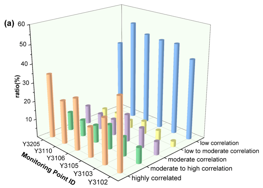
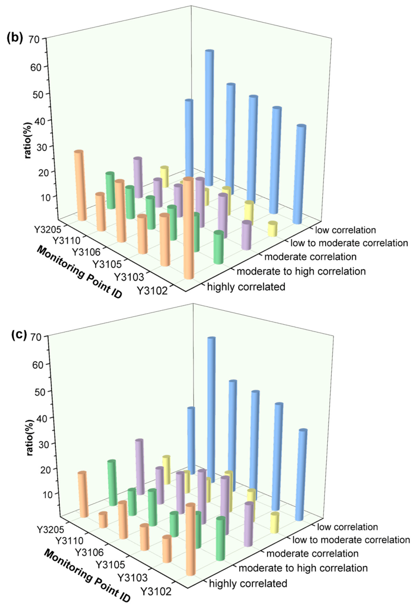
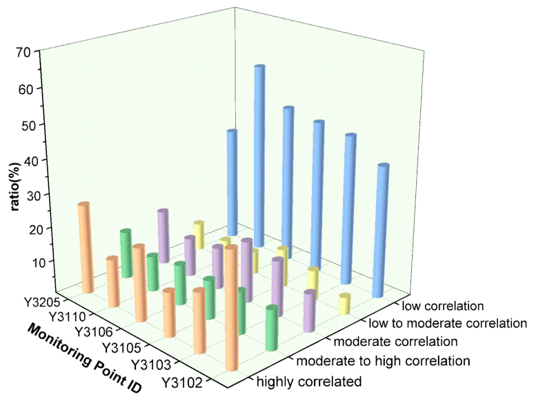
Building on the monitoring setup and site characteristics described in Section 2.1, this section presents the annual correlation statistical results of the Shaxi–Qijiang Highway pilot zone, as illustrated in Figure 4.

Based on the annual correlation statistical results output by the model, the correlation distribution exhibits significant time-scale effects and spatial heterogeneity.

(1) Time-Scale Effect Analysis: Taking monitoring point Y3102 as an example, in the 2 h window, the mean proportion of high correlation is 38.2%, with low correlation at 43.0%. In the 6 h window, high correlation drops to 35.4%, and low correlation decreases to 38.4%. In the 12 h window, high correlation further declines to 25.3%, while medium–high correlation rises to 15.5% and low correlation falls to 35.7%. The data indicate that as the time window expands, the proportion of high correlation shows a decreasing trend, whereas medium–high correlation increases and low correlation decreases accordingly. This is attributed to the fact that longer windows can integrate more systemic hydraulic trend components, effectively smoothing out the impact of short-term local disturbances on the correlation degree. The chi-square test of independence for Y0201 yielded χ² = 307.2, df = 8, p < 0.001, with a Cramer’s V of 0.226 indicating a moderate effect size; post hoc residuals confirm that the 12 h window elevates medium correlations by 103% relative to expectations, validating the smoothing effect of longer windows. In the statistical results for monitoring point Y3110, the data—showing 60.7% low correlation at 2 h versus 40.4% at 12 h—further validated the integration and enhancement effect of long windows on weak correlation signals.

(2) Spatial Heterogeneity Analysis: The overall mean proportion of high correlation at monitoring point Y3102 is significantly higher than that of points such as Y3103 and Y3110, which is consistent with its characteristics as a core node of the sewage main with strong hydraulic connectivity. In the case of Y3205, the proportion of low correlation during the rainy season is only 21.3%, far lower than other monitoring points during the same period. This indicates that the hydraulic coupling effect between this pipe segment and the river is significantly intensified during the rainy season.

The overall correlation level proportions for the six monitoring points in the Shaxi–Qijiang Highway section are shown in Figure 5. The area is characterized primarily by low correlation (mean proportion of 44.57%), though spatial differentiation is distinct. Monitoring points along the main pipe, such as Y3102 and Y3205, exhibit strong correlation (high + medium–high) proportions of 44.8% and 41.0%, respectively, marking them as high-risk zones for I/I intrusion. Conversely, terminal branch points like Y3110 show a low correlation proportion as high as 56.9%, representing the lowest risk. These quantitative results provide a direct basis for decision-making regarding hierarchical control and precision operation and maintenance of the regional pipe network.

3.2. Application Analysis of the Yicheng Catchment

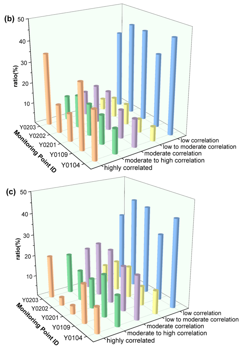
Building on the monitoring setup and site characteristics of the Yicheng Area described in Section 2.1, this section presents the annual correlation statistical results of this pilot zone, as illustrated in Figure 6.

The annual correlation statistical results for the Yicheng catchment further reveal the synergistic influence of window size and displacement constraints.

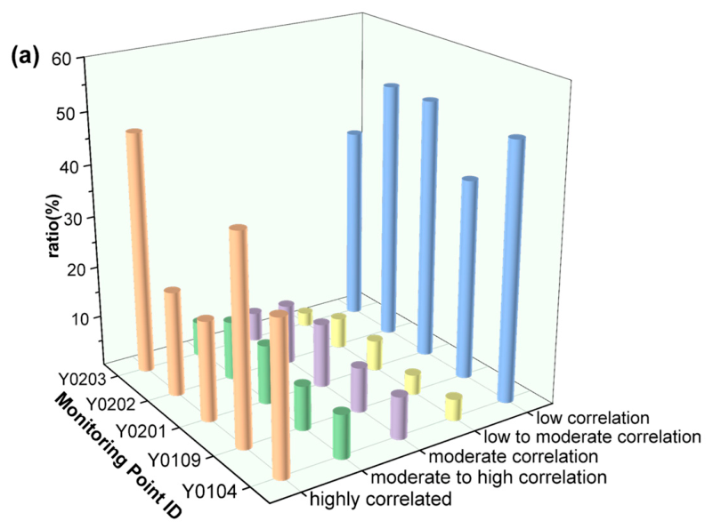
(1) Synergistic Effects of Time-Scale and Displacement Constraints: Taking Y0109 as an example, under the condition of a 6 h window and a 2 h displacement constraint, the proportion of high correlation is 35.6% and medium–high correlation is 14.7%. In contrast, under a 2 h window with the same displacement constraint, high correlation rises to 40.0%, but low correlation also reaches 38.7%. This comparison indicates that a 6 h window paired with a 2 h displacement constraint is more effective for extracting medium-high correlation components. This aligns with the actual hydraulic lag of the catchment (approximately 1–2 h), effectively smoothing out instantaneous disturbances while capturing trend-based correlations. Data from Y0202 further corroborate this: the combination of a 12 h window with a 2 h displacement constraint yielded a combined high and medium–high correlation proportion of 48.6%, significantly outperforming the 1 h constraint combination (<30%). This suggests that moderately relaxing displacement constraints can enhance the identification accuracy of long-duration windows.

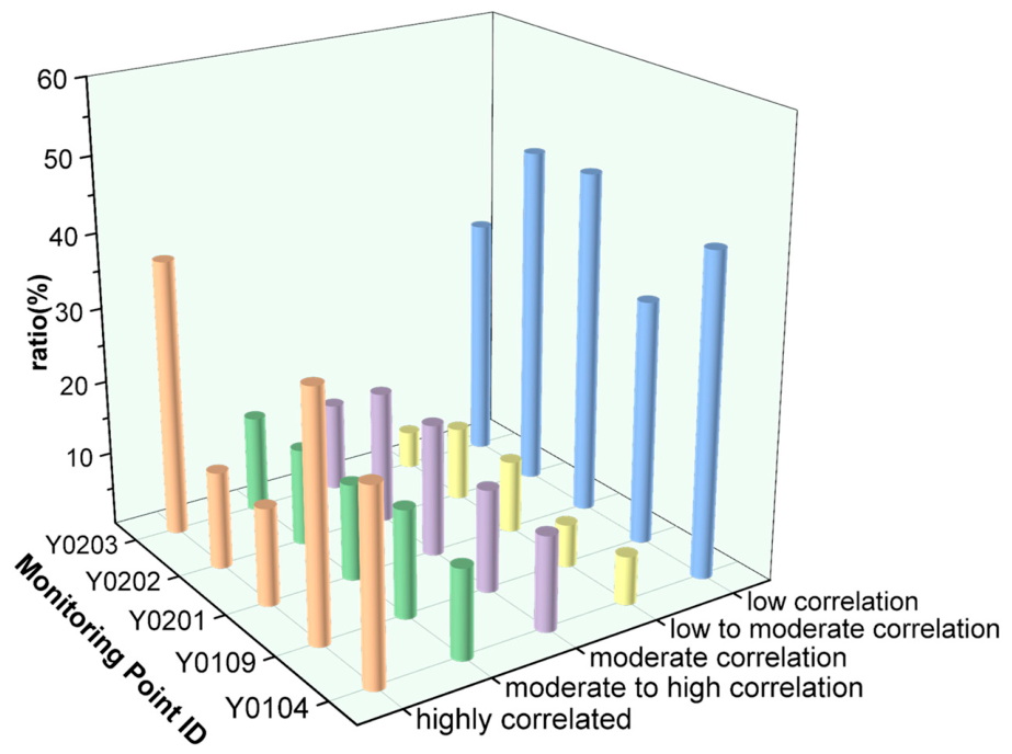
(2) Spatial Heterogeneity Analysis: The overall proportions of correlation levels are shown in Figure 7. While the average proportion of low correlation in the catchment is 39.92%, spatial differentiation remains significant. Monitoring points along the main pipes, such as Y0109 and Y0203, exhibit strong correlation (high + medium–high) proportions of 47.6% and 50.3%, respectively, identifying them as high-risk zones for I/I intrusion; conversely, points Y0201 and Y0202 show low correlation proportions exceeding 45% with a combined strong correlation of less than 30%, indicating a lower risk. These results provide a quantitative basis for differentiated risk management and control within the catchment.

3.3. Model Adaptability Verification

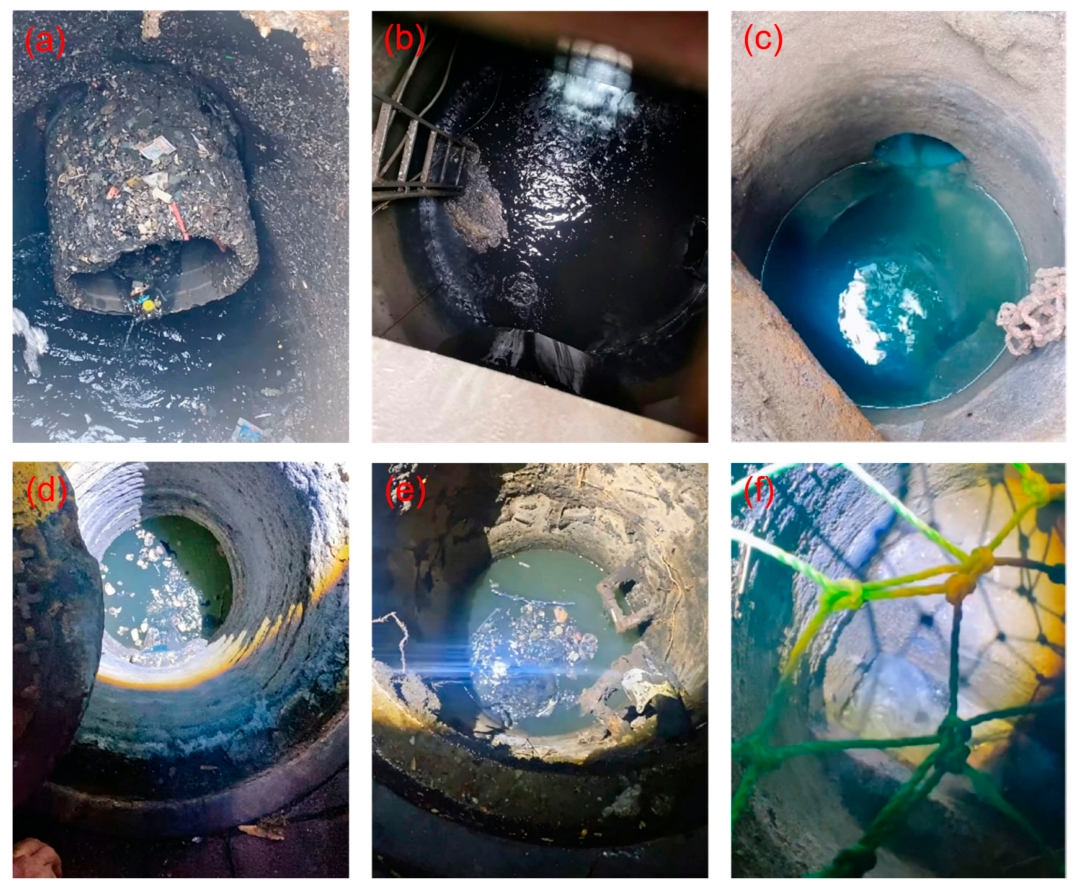
To further verify the model’s generalization capability and field applicability, six monitoring points (Y2901, Y3101, Y1602, Y0902, YB106, and Y0107) were randomly selected for screening. Among these, five were identified as highly correlated and one as moderately correlated. Following the model’s analysis indicating potential I/I intrusion near these points, the project team commissioned field personnel to conduct detailed on-site investigations. Various methods, including manhole inspections, water quality and odor assessment, flow direction confirmation, and environmental audits (see Figure 8), were employed to determine the actual presence of I/I intrusion.

Field verification revealed a total of six I/I intrusion points (including seepage, aged gates, and rainwater I/I) in the vicinity of the five high-correlation points, achieving a hit rate of 83.3%. No explicit intrusion points were identified near the medium-correlation point, which may be attributed to the complex nature of the combined drainage system in the old urban area [35]. These validation results demonstrate that the model possesses excellent universality and field applicability. It should be noted that while the hit rate in this verification batch reached 83.3%, the sample size (n = 6) is relatively limited; further large-scale validation is recommended to confirm the generalizability of the model.

4. Conclusions

This study constructed a multi-scale river–pipe network water level correlation analysis model based on the fusion of DTW, Pearson, and Spearman coefficients. By employing a three-level fusion architecture, dynamic weight allocation, and strategies involving multi-scale windows and displacement constraints, the model achieved a comprehensive and precise assessment of the correlation characteristics between river and pipe network water levels. The model was validated and applied in the Shaxi–Qijiang Highway section and the Yicheng catchment of a city in southern China. The primary conclusions are as follows:

(1) The model’s recognition accuracy and scenario adaptability were verified using a validation dataset comprising 36 typical water-level sequences (12 groups per category), achieving classification accuracies of 91.7% for the low-correlation category and perfect classification (100%) for both medium- and high-correlation categories. This demonstrates that the framework effectively eliminates the confounding impacts of temporal asynchrony, nonlinear hydraulic dynamics, and data anomalies.

(2) The model precisely captures the temporal periodicity, window scale effects, and spatial heterogeneity of the river–pipe network water level relationship. Crucially, in separate sewer systems, the detection of medium-to-high correlation during dry weather serves as a direct and sensitive indicator of illicit sewer–river connections or unintended river backflow, offering a distinct advantage over traditional inspection methods.

(3) In practical applications, the model demonstrates high recognition precision and universality. It successfully identified multiple high-risk pipe segments for I/I intrusion in the Shaxi–Qijiang Highway section and Yicheng catchment, with a field verification hit rate of 83.3% in the test batch, providing accurate technical guidance for intrusion troubleshooting.

(4) This model introduces a robust data-driven approach for identifying hydraulic anomalies in urban drainage systems. Beyond the combined system scenarios demonstrated herein, its core logic is particularly valuable for separate sewer systems to detect illicit discharges and prevent clean water inflow. It significantly reduces manual inspection costs and enhances O&M efficiency, providing scientific support for refined drainage management and holding substantial practical value for improving urban water environments.

References

1. Chadfield, S.J.; Wei, Y.P.; Lieske, S.N. Water sensitive communities: A systematic review with a complex adaptive systems perspective. J. Environ. Plan. Manag. 2024, 67, 1077–1103. [Google Scholar] [CrossRef]
2. Zhang, H.; Jia, H.; Mels, A.; Rijnaarts, H.; Chen, W.-S. Extraneous water in sewer systems: A comprehensive review on sewer infiltration and inflow quantification, localization and mitigation. Water Res. X 2025, 29, 100426. [Google Scholar] [CrossRef]
3. Rezaee, M.; Tabesh, M. Effects of inflow, infiltration, and exfiltration on water footprint increase of a sewer system: A case study of Tehran. Sustain. Cities Soc. 2022, 79, 103707. [Google Scholar] [CrossRef]
4. Zhang, M.K.; Liu, Y.C.; Cheng, X.; Zhu, D.Z.; Shi, N.C.; Yuan, Z.G. Quantifying rainfall-derived inflow and infiltration in sanitary sewer systems based on conductivity monitoring. J. Hydrol. 2018, 558, 174–183. [Google Scholar] [CrossRef]
5. Bai, Y.; Xu, A.; Wu, Y.H.; Xue, S.; Chen, Z.; Hu, H.Y. Portrait of municipal wastewater of China: Inspirations for wastewater collection, treatment and management. Water Res. 2025, 277, 123321. [Google Scholar] [CrossRef] [PubMed]
6. Guo, S.; Shi, X.; Luo, X.J.; Yang, H.M. River water intrusion as a source of inflow into the sanitary sewer system. Water Sci. Technol. 2020, 82, 2472–2481. [Google Scholar] [CrossRef] [PubMed]
7. Karpf, C.; Krebs, P. Quantification of groundwater infiltration and surface water inflows in urban sewer networks based on a multiple model approach. Water Res. 2011, 45, 3129–3136. [Google Scholar] [CrossRef] [PubMed]
8. Song, W.; Fang, H.Z.; Lei, Z.S.; Wang, R.G.; Fu, C.X.; Wang, F.; Fang, Y.N.; Du, X.; Wang, Z.H.; Zhao, Z.W. Insight into homogeneous activation of sodium hypochlorite by dithionite coupled with dissolved oxygen (DO@NaClO/DTN) for carbamazepine degradation. Water Res. 2025, 277, 123312. [Google Scholar] [CrossRef] [PubMed]
9. Beheshti, M.; Sægrov, S. Detection of extraneous water ingress into the sewer system using tandem methods—A case study in Trondheim city. Water Sci. Technol. 2019, 79, 231–239. [Google Scholar] [CrossRef] [PubMed]
10. Song, W.; Fang, H.Z.; Zhang, Z.T.; Fu, C.X.; Du, X.; Liu, B.Z.; Li, B.; Wang, R.G.; Huang, C.Y.; Wang, Z.H.; et al. Mechanistic role of chloride in enhancing carbamazepine degradation by dithionite-activated sodium hypochlorite. J. Hazard. Mater. 2026, 501, 140947. [Google Scholar] [CrossRef] [PubMed]
11. Fang, X.; Guo, W.H.; Li, Q.Q.; Zhu, J.S.; Chen, Z.P.; Yu, J.W.; Zhou, B.D.; Yang, H.K. Sewer Pipeline Fault Identification Using Anomaly Detection Algorithms on Video Sequences. IEEE Access 2020, 8, 39574–39586. [Google Scholar] [CrossRef]
12. Wang, M.N.; Liu, Y. Recent advances in smart water technology of drainage systems in China. Water Int. 2023, 48, 379–392. [Google Scholar] [CrossRef]
13. Wei, Q.; Qi, Y.; Chen, Y.Q.; Xie, Y.F.; Yin, H.L.; Xu, Z.X. Data-driven interpretation of overflow pollution mechanism of urban drainage system using automated machine learning model. J. Water Process Eng. 2025, 77, 108482. [Google Scholar] [CrossRef]
14. Cheng, M.; Evangelisti, M.; Gobeyn, S.; Avolio, F.; Frascari, D.; Maglionico, M.; Ciriello, V.; Di Federico, V. Establishing correlations between time series of wastewater parameters under extreme and regular weather conditions. J. Hydrol. 2025, 649, 132455. [Google Scholar] [CrossRef]
15. van Daal-Rombouts, P.; Sun, S.; Langeveld, J.; Bertrand-Krajewski, J.L.; Clemens, F. Design and performance evaluation of a simplified dynamic model for combined sewer overflows in pumped sewer systems. J. Hydrol. 2016, 538, 609–624. [Google Scholar] [CrossRef]
16. Woo, H.; Boccelli, D.L.; Uber, J.G.; Janke, R.; Su, Y. Dynamic Time Warping for Quantitative Analysis of Tracer Study Time-Series Water Quality Data. J. Water Resour. Plan. Manag. 2019, 145, 04019028. [Google Scholar] [CrossRef]
17. Stübinger, J.; Walter, D. Using Multi-Dimensional Dynamic Time Warping to Identify Time-Varying Lead-Lag Relationships. Sensors 2022, 22, 6884. [Google Scholar] [CrossRef] [PubMed]
18. Zhang, M.Q.; Li, W.Z.; Zhang, L.; Jin, H.; Mu, Y.S.; Wang, L. A Pearson correlation-based adaptive variable grouping method for large-scale multi-objective optimization. Inf. Sci. 2023, 639, 119361. [Google Scholar] [CrossRef]
19. Ma, L.; Liu, Z.B.; Chen, W.M.; Hu, J.J.; Ye, H.J.; Fan, T.; An, L. Coal Mine Water Inflow Prediction Model Based on Multi-Factor Pearson Correlation Analysis. Appl. Sci. 2025, 15, 6600. [Google Scholar] [CrossRef]
20. Zhu, B.; Yuan, J.Q. Pressure transfer modeling for an urban water supply system based on Pearson correlation analysis. J. Hydroinformatics 2015, 17, 90–98. [Google Scholar] [CrossRef]
21. Qin, X.L.; Wang, L.; Li, X.H.; Yu, H.; Wang, K.; Fan, D.F. Regional Characteristics of Precipitation in the Nanpan River Basin, China. Front. Environ. Sci. 2022, 9, 783515. [Google Scholar] [CrossRef]
22. Abd Al-Hameeda, K.A. Spearman’s correlation coefficient in statistical analysis. Int. J. Nonlinear Anal. Appl. 2022, 13, 3249–3255. [Google Scholar] [CrossRef]
23. Sugihara, G.; May, R.; Ye, H.; Hsieh, C.H.; Deyle, E.; Fogarty, M.; Munch, S. Detecting Causality in Complex Ecosystems. Science 2012, 338, 496–500. [Google Scholar] [CrossRef] [PubMed]
24. Hatt, B.E.; Fletcher, T.D.; Walsh, C.J.; Taylor, S.L. The influence of urban density and drainage infrastructure on the concentrations and loads of pollutants in small streams. Environ. Manag. 2004, 34, 112–124. [Google Scholar] [CrossRef] [PubMed]
25. Jasinski, R. The use of interpolation methods for the modelling of environmental data. Desalin. Water Treat. 2016, 57, 964–970. [Google Scholar] [CrossRef]
26. Zhang, X.Y.; Colicino, E.; Cowell, W.; Enlow, M.B.; Kloog, I.; Coull, B.A.; Schwartz, J.D.; Wright, R.O.; Wright, R.J. Prenatal exposure to air pollution and BWGA Z-score: Modifying effects of placenta leukocyte telomere length and infant sex. Environ. Res. 2024, 246, 117986. [Google Scholar] [CrossRef] [PubMed]
27. Huang, H.D.; Zhang, Z.X.; Song, F.X. An Ensemble-Learning-Based Method for Short-Term Water Demand Forecasting. Water Resour. Manag. 2021, 35, 1757–1773. [Google Scholar] [CrossRef]
28. Stasiak, B.; Skiba, M.; Niedzielski, A. FlatDTW—Dynamic Time Warping optimization for piecewise constant templates. Digit. Signal Process. 2019, 85, 86–98. [Google Scholar] [CrossRef]
29. Teng, Y.R.; Wang, G.T.; He, C.L.; Wu, Y.Y.; Li, C.R. Optimization of Dynamic Time Warping Algorithm for Abnormal Signal Detection. Int. J. Data Sci. Anal. 2025, 19, 115–127. [Google Scholar] [CrossRef]
30. Geler, Z.; Kurbalija, V.; Radovanovic, M.; Ivanovic, M. Impact of the Sakoe-Chiba Band on the DTW Time-Series Distance Measure for kNN Classification. In Lecture Notes in Artificial Intelligence, Proceedings of the 7th International Conference on Knowledge Science, Engineering and Management (KSEM), Sibiu, Romania, 16–18 October 2014; Springer: Berlin, Germany; Lucian Blaga University of Sibiu, Faculty of Engineering: Sibiu, Romania, 2014; pp. 105–114. [Google Scholar]
31. Pranowo, W.; Ramadhani, A.R. Error-based correlation coefficient: An alternative to combine error and coefficient of correlation and its application in geophysical data. J. Comput. Sci. 2025, 88, 102611. [Google Scholar] [CrossRef]
32. Xu, W.C.; Hou, Y.H.; Hung, Y.S.; Zou, Y.X. A comparative analysis of Spearman’s rho and Kendall’s tau in normal and contaminated normal models. Signal Process. 2013, 93, 261–276. [Google Scholar] [CrossRef]
33. Song, X.Y.; Xia, X.H.; Luan, F.J. Online Signature Verification Based on Stable Features Extracted Dynamically. IEEE Trans. Syst. Man. Cybern. Syst. 2017, 47, 2663–2676. [Google Scholar] [CrossRef]
34. Filion, Y.; Adams, B.; Karney, B. Cross correlation of demands in water distribution network design. J. Water Resour. Plan. Manag. 2007, 133, 137–144. [Google Scholar] [CrossRef]
35. Möderl, M.; Kleidorfer, M.; Rauch, W. Influence of characteristics on combined sewer performance. Water Sci. Technol. 2012, 66, 1052–1060. [Google Scholar] [CrossRef] [PubMed]
Figure 1. Route map of sewage pipes on the Shaxi–Qijiang Highway section.
Water 18 01811 g001
Figure 2. Distribution map of experimental sites in Baishiyong—an urban area.
Water 18 01811 g002
Figure 3. Structure diagram of the fusion algorithm.
Water 18 01811 g003
Figure 4. The annual statistical results of data from the Shaxi–Qijiang Highway section concerning the correlation proportion under (a) a 2 h time window, (b) a 6 h time window, and (c) a 12 h time window.
Water 18 01811 g004aWater 18 01811 g004b
Figure 5. Statistics on the proportion of correlation levels between the Baishiyong River and pipeline water levels in the Shaxi–Qijiang Highway section.
Water 18 01811 g005
Figure 6. The annual statistical results of correlation proportions under varying time windows and displacement constraints for the Yicheng Area: (a) a 2 h window; (b) a 6 h window; (c) a 12 h window.
Water 18 01811 g006aWater 18 01811 g006b
Figure 7. Statistics on the proportion of correlation levels between the Baishiyong River and pipeline water levels in the Yicheng Area.
Water 18 01811 g007
Figure 8. On-site inspection photos of I/I intrusion points: (a) I/I intrusion points around the level gauge of the Y2901 Xinggang Road sewer main; (b) I/I intrusion points around the level gauge of the Y3101 Qijiang Highway sewer main (south); (c) I/I intrusion points around the level gauge of the Y1602 Qingxi Road sewer main; (d) I/I intrusion point 1 around the level gauge of the Y0902 Minke West Road sewer main; (e) I/I intrusion point 2 around the level gauge of the Y0902 Minke West Road sewer main; (f) I/I intrusion points around the level gauge of the YB106 Yanjiang Road sewer main.
Water 18 01811 g008