Hydrological Performance of Uncorrected CORDEX-SA Climate Model Outputs Across Glacier, Snow and Rain–Snow Regimes in the Upper Indus Basin

Abstract

Six river basins of the Upper Indus Basin (UIB), Pakistan, representing glacier-dominated (Hunza and Shyok), snow-dominated (Gilgit, Chitral, and Astore), and rain–snow-mixed (Swat) hydroclimatic regimes are examined to evaluate the suitability of uncorrected CORDEX-SA climate data for hydrological modelling. Data scarcity and complex high-mountain topography make it difficult to obtain reliable inputs, and although bias correction is widely applied to regional climate model (RCM) outputs, it can distort the climate signal and introduce additional uncertainties. This study investigates the extent to which uncorrected outputs from the CORDEX South Asia ensemble can directly simulate daily streamflow in a data-scarce mountainous environment. Nine GCM–RCM combinations, comprising five global climate models and three regional climate models (COSMO-crCLIM-v1-1, REMO2015, and RegCM4-7), are used to drive the HBV-IANIGLA snow–glacier hydrological model over 1981–2005, with calibration from 1981 to 1999 and validation from 2000 to 2005. Several CORDEX-SA members reproduce daily streamflow with acceptable skill without bias correction, but performance is strongly regime-dependent. Snow-dominated basins perform best, followed by glacier-dominated basins, while the rain–snow-mixed basin remains most challenging. COSMO-crCLIM-v1-1 and RegCM4-7 outperform REMO2015 on average. The results indicate that uncorrected CORDEX-SA members can support hydrological assessments in snow-dominated catchments, whereas glacier-dominated and monsoon-influenced basins require additional treatment of climate forcing.

1. Introduction

The Hindukush–Karakoram–Himalaya (HKH) region, often referred to as the “Third Pole” because of its large stores of snow and glacial ice [1,2,3], is the source of several major Asian rivers, including the Indus, Ganges and Brahmaputra, that together supply freshwater to about a billion people [4]. The Indus is of particular regional importance, hosting the Indus Basin Irrigation System, one of the largest in the world, which supports more than 90% of Pakistan’s agricultural production and meets most of the country’s water demand [5,6]. Within the Indus system, the Upper Indus Basin (UIB) feeds the Tarbela Reservoir, contributing 60–80% of the total annual flow through snow and glacier melt [5,7,8,9]. A recent process-based simulation covering the 1951–2019 period estimated that combined snow and glacier melt account for approximately 65% of total runoff in the UIB, with snowmelt dominating spring runoff and glacier melt providing roughly 15% of total summer flow [10].

Climate change is a major threat to mountain hydrology, particularly in the UIB, where the streamflow regime is strongly dependent on cryospheric processes [11,12]. Glacier responses in the basin are spatially heterogeneous. While glaciers in the Himalayan parts of the basin have generally lost mass in recent decades, many Karakoram glaciers have remained close to mass balance [7]. Recent assessments of future projections show that glaciers of different sizes respond differently to climate forcing, with large glaciers projected to sustain a substantial share of future runoff while small glaciers disappear earlier [13]. Coupled with shifts in precipitation phase and earlier snowmelt onset [10,14], these processes introduce considerable uncertainty regarding future water availability across the UIB.

Accurate modelling of UIB climate and hydrology is strongly constrained by the scarcity of observational data. Meteorological stations are concentrated at low elevations and do not capture precipitation gradients occurring above 3000 m [10,15,16], while several gridded products are known to underestimate high-altitude precipitation [7,9]. Combined with rugged topography, logistical access difficulties and short observational records, these data gaps result in substantial uncertainties in glacier mass balance, snow cover and streamflow estimates [17,18,19]. Consequently, hydrological modelling in the UIB depends heavily on the quality of the climate forcing data employed.

Climate models are the main tool used to quantify how the climate system responds to natural and anthropogenic forcing [20,21,22]. Global climate models (GCMs) provide such information at coarse spatial resolutions, which are generally too coarse for hydrological assessments in mountainous catchments. To improve regional representation, the Coordinated Regional Climate Downscaling Experiment (CORDEX) provides dynamically downscaled outputs from different GCM–RCM combinations across fourteen continental domains and has been widely utilised in climate change impact studies [21,23]. CORDEX outputs have, for example, been applied to drought projections in northern Italy [24] and to assess future climate indices for Nepal under multiple emission scenarios [25]. For the South Asia domain, the CORDEX-SA ensemble is the most widely utilised downscaled product for the UIB and surrounding region, with several studies having employed it to project future precipitation, temperature and snowmelt-driven runoff [9,14,26,27,28].

Despite numerous modelling studies, three topics remain underexplored within the context of the UIB. First, most existing studies rely on a single GCM or RCM, which limits the assessment of model uncertainty and may introduce biases in resulting conclusions [29,30]. Second, where multi-model ensembles are utilised, performance is rarely compared across contrasting hydrological regimes within the same basin, even though glacier-dominated, snow-dominated and rain–snow-mixed catchments respond differently to uniform climate forcing [10,28,31]. Third, RCM outputs are routinely bias-corrected before being used as hydrological forcing [26,32,33]; however, bias correction itself can significantly distort climate change signals, alter non-stationary features, and introduce new uncertainties into the simulated discharge [28,34,35,36]. Whether raw (uncorrected CORDEX-SA) outputs alone can reliably support hydrological simulation in the UIB has not been systematically evaluated. Addressing this knowledge gap is operationally relevant because reliable hydrological modelling is essential for water-resource planning in a country highly vulnerable to climate change [37,38].

The HBV-IANIGLA model was selected for several reasons. It effectively simulates snow accumulation and melt, as well as the melting of both clean and debris-covered glacier ice, using a relatively small set of physically interpretable parameters. This makes it particularly suitable for the Karakoram region, where glaciers occupy a substantial portion of many catchments. The model requires only daily precipitation, temperature, and potential evapotranspiration as inputs, making it well suited for the data-limited conditions of the Upper Indus Basin (UIB). It has also been successfully applied in other mountainous basins dominated by snow and glacier processes. Furthermore, its open-source implementation in R ensures reproducibility and enables direct application with the daily CORDEX-SA climate forcing used in this study. More complex, fully distributed hydrological models and purely data-driven (machine learning) approaches were considered less appropriate, as the primary objective of this research is to evaluate the quality of the climate forcing rather than to investigate hydrological model structure.

The aims of this study are to evaluate whether uncorrected CORDEX-SA outputs can be used as direct hydrological forcing in the UIB and to identify which GCM–RCM combinations perform best across different hydroclimatic regimes. Nine CORDEX-SA members combining five GCMs and three RCMs (COSMO-crCLIM-v1-1, REMO2015, RegCM4-7) are employed to drive the conceptual snow–glacier model HBV-IANIGLA across six UIB sub-basins representing glacier-dominated (Hunza and Shyok), snow-dominated (Gilgit, Chitral, and Astore) and rain–snow-mixed (Swat) regimes [39]. The key objectives of this study are (1) to quantify the runoff model performance of each CORDEX-SA member against observed daily streamflow over the calibration (1981–1999) and validation (2000–2005) periods; (2) to assess how this performance varies across the three contrasting hydroclimatic regimes; and (3) to identify CORDEX-SA members that demonstrate temporal stability in performance across both periods and could therefore support climate-impact assessments in the UIB and similar data-scarce, glacier-influenced basins.

2. Materials and Methods

2.1. Study Area

The Upper Indus Basin (UIB) covers the high-altitude portion of the Indus Basin, originating in the Tibetan Plateau and the Hindukush–Karakoram–Himalaya region [40]. The climate of the basin is governed by two large-scale circulation systems: the Indian summer monsoon, which dominates from June to September, and the mid-latitude westerlies, whose winter and spring western disturbances deliver the majority of precipitation to the western and northern parts of the basin [15,41]. This dual control produces strong spatial heterogeneity in precipitation dynamics and snowpack accumulation across the UIB.

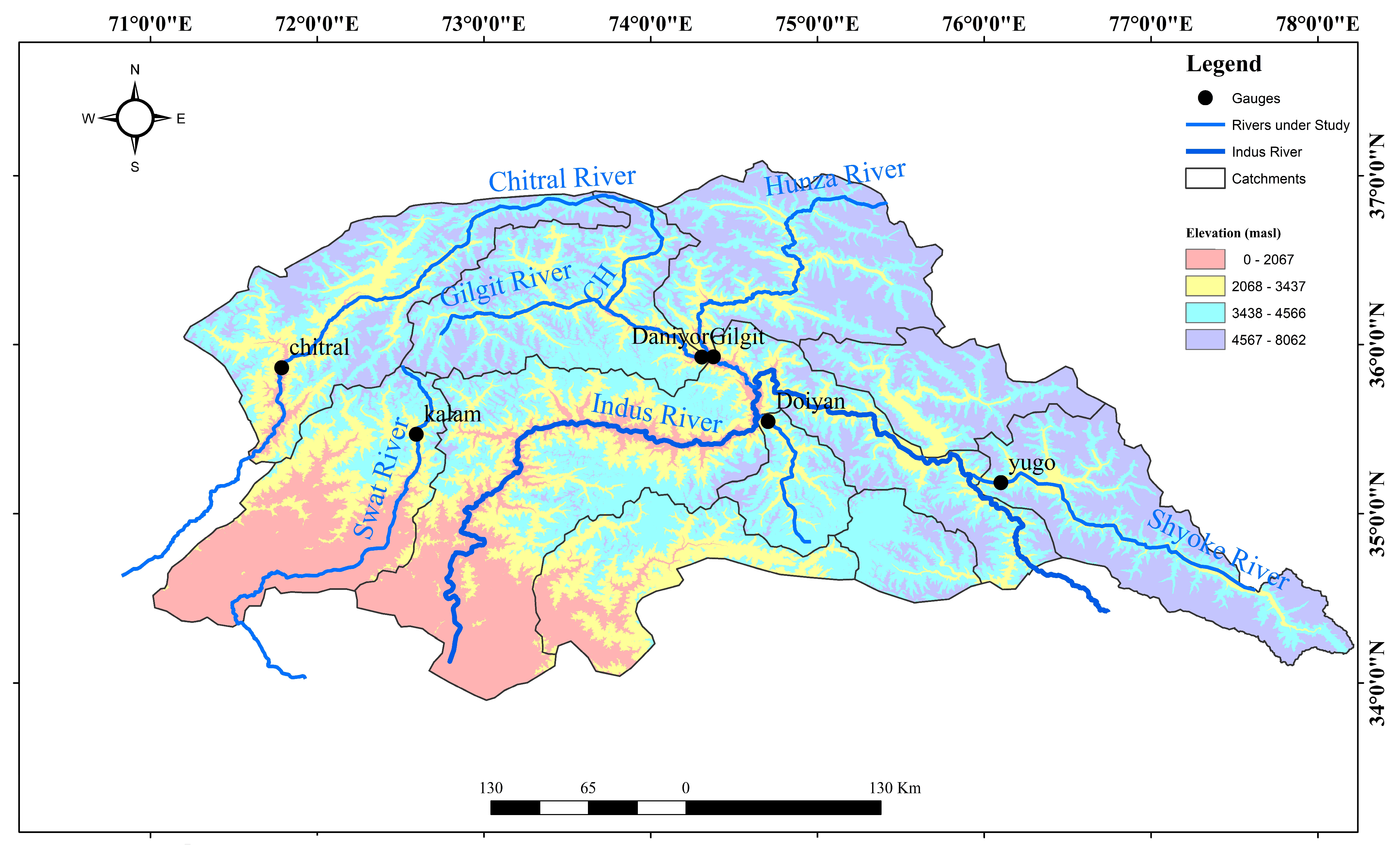
Six sub-basins of the UIB were selected to represent the three dominant hydroclimatic regimes of the region [39]: two glacier-dominated catchments (Hunza and Shyok) draining the high Karakoram range, three snow-dominated catchments (Gilgit, Chitral, and Astore) where seasonal snowmelt is the main driver of streamflow, and one rain–snow-mixed catchment (Swat) where monsoonal rainfall contributes substantially in addition to snowmelt [42,43,44,45]. Glacier coverage decreases from about 35% in Hunza and Shyok to less than 4% in Swat (

Table 1. Hydroclimatic regime and physiographic characteristics of the six analysed sub-basins.

Basin	Hunza	Shyok	Gilgit	Chitral	Astore	Swat
Regime	Glacier-dominated	Glacier-dominated	Snow-dominated	Snow-dominated	Snow-dominated	Rain–snow-mixed
Dominant runoff driver	Glacier melt	Glacier melt	Seasonal snowmelt	Seasonal snowmelt	Seasonal snowmelt	Monsoon rainfall + snowmelt
Gauge latitude (°N)	35.93	35.18	35.93	35.86	35.55	35.47
Gauge longitude (°E)	74.38	76.10	74.31	71.79	74.70	72.59
Area (km2)	13,100	10,235	14,800	11,396	3927	5745
Mean basin elevation (m a.s.l.)	3800	3200	4230	2800	3500	2600
Glacier coverage (%)	35.0	34.7	14.0	10.0	8.0	3.5

). Sub-basin areas were delineated from the ASTER Global Digital Elevation Model (ASTER GDEM) at 30 m resolution. The location and topography of the six sub-basins are shown in Figure 1.

2.1.1. Hydrological Data

Daily observed streamflow data for the six study basins (Hunza, Shyok, Gilgit, Chitral, Astore and Swat; Figure 1) were used to calibrate and validate the hydrological model. These streamflow records were provided by the Water and Power Development Authority (WAPDA) of Pakistan. The available dataset covers the period 1981–2005, matching the historical CORDEX-SA output described in Section 2.1.2.

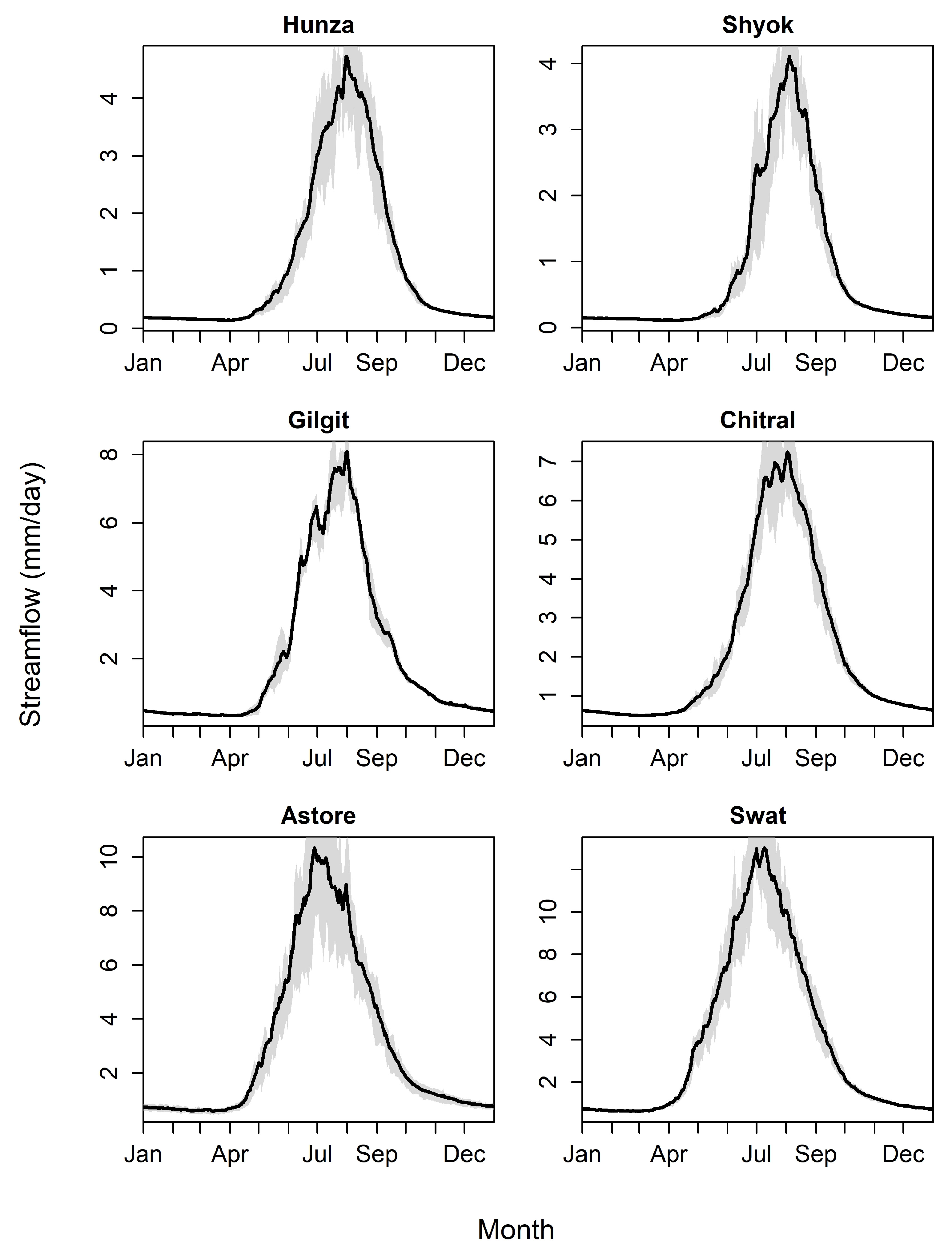
Figure 2 shows the mean monthly regime curves of the six sub-basins for the period 1981–1999. All basins exhibit low discharge between January and April, corresponding to frozen storage conditions and limited melt. Discharge starts to rise in late spring as snowmelt begins and reaches its peak between July and August, when glacier melt and (in the rain–snow basin) monsoon rainfall are at their maximum. Glacier-dominated basins (Hunza and Shyok) show a pronounced and narrow summer peak, consistent with a temperature-driven melt regime. The snow-dominated basins (Gilgit, Chitral, and Astore) display a slightly broader peak that reflects a combination of seasonal snowmelt and moderate glacier melt. The rain–snow-mixed basin (Swat) exhibits higher summer flows that follow monsoon precipitation more closely, with greater intra-seasonal variability.

2.1.2. CORDEX-SA Data

Daily precipitation and near-surface air temperature outputs from nine GCM–RCM members of the CORDEX South Asia (CORDEX-SA, also termed CORDEX-WAS in the database of World Climate Research Programme) experiment were obtained from the Earth System Grid Federation node hosted at the German Climate Computing Center (https://esgf-data.dkrz.de/search/esgf-dkrz/, accessed on 5 January 2026) for the historical period 1981–2005. The members pair six GCMs (MPI-ESM-LR, MPI-ESM-MR, NorESM1-M, EC-EARTH, HadGEM2-ES, and MIROC5) with three RCMs (COSMO-crCLIM-v1-1, REMO2015 and RegCM4-7), as listed in

Table 2. CORDEX-SA model members used in the hydrological modelling. Each member combines a single global climate model (GCM) and a single regional climate model (RCM). Members are grouped by driving GCM (MPI-M first, NCC second, mixed third) and ordered within each group by RCM (COSMO → REMO → RegCM4-7). The ID column gives the abbreviation used throughout the text.

ID	GCM	RCM
M1	MPI-M-MPI-ESM-LR	COSMO-crCLIM-v1-1
M2	MPI-M-MPI-ESM-LR	REMO2015
M3	MPI-M-MPI-ESM-MR	RegCM4-7
M4	NCC-NorESM1-M	COSMO-crCLIM-v1-1
M5	NCC-NorESM1-M	REMO2015
M6	NCC-NorESM1-M	RegCM4-7
M7	ICHEC-EC-EARTH	COSMO-crCLIM-v1-1
M8	MOHC-HadGEM2-ES	REMO2015
M9	MIROC-MIROC5	RegCM4-7

. All outputs are provided on a regular grid of 0.22° (approximately 25 km). The choice of the 1981–2005 window was constrained by the temporal availability of CORDEX-SA historical runs, which end in 2005. Catchment-mean daily precipitation and air temperature were extracted in R [46] by overlaying the catchment boundaries on the CORDEX-SA grid using an area-weighted averaging [47].

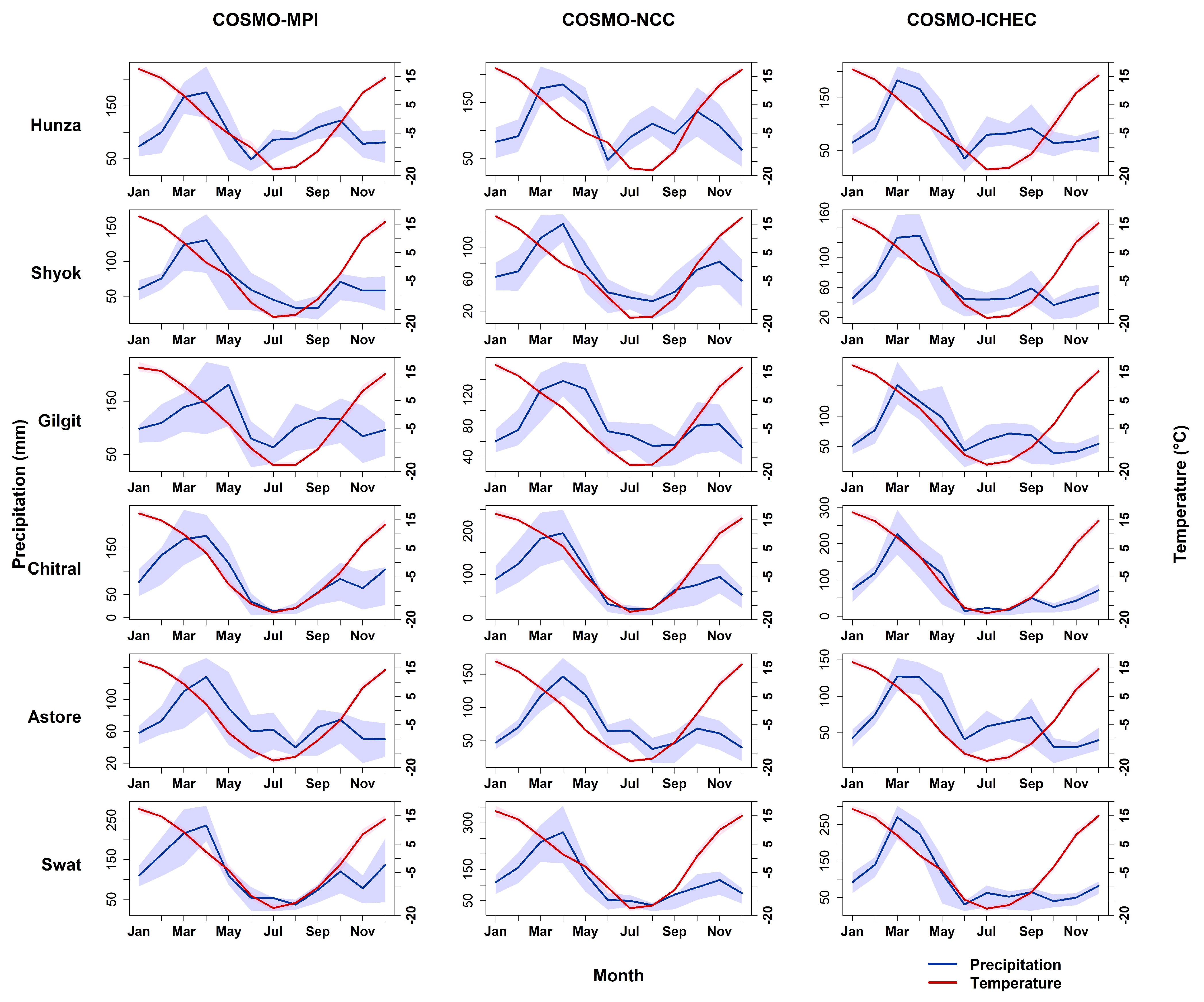
Figure 3 presents an example of the monthly climatology of precipitation and near-surface air temperature for the six study sub-basins during the calibration period, using three representative CORDEX SA members driven by the COSMO RCM-crCLIM-v1-1. Corresponding plots for the other analysed CORDEX-SA members are presented in the Supplementary Material (Figures S1 and S2). Figure 3 shows that across the glacier-dominated basins, air temperature seasonality exhibits a sharp summer peak, while precipitation remains relatively low throughout the year. In the snow-dominated basins, precipitation is more evenly distributed across the seasons and discharge rises earlier and more gradually in spring (Figure 2), in response to the seasonal temperature increase and subsequent snowmelt. In the rain–snow-mixed basin (Swat), precipitation and discharge peak concurrently in July–August, reflecting the direct contribution of monsoon rainfall. The inter-quartile range of monthly precipitation and air temperature (shaded bands) show that the variability is the largest in the rain–snow-mixed basin and smallest in the snow-dominated basins.

2.2. Methods

2.2.1. Hydrological Model

Streamflow in the six sub-basins was simulated using HBV-IANIGLA, an extension of the conceptual rainfall–runoff model HBV (Hydrologiska Byråns Vattenbalansavdelning) [48,49,50] that adds explicit modules for clean and debris-covered glacier mass balance and glacier meltwater routing [51]. The model partitions the catchment-mean daily climate forcing into snow, soil-moisture and groundwater stores. The modelled runoff generation processes include partitioning of precipitation into rain and snow, snow accumulation and melt, glacier mass balance and ice melt, soil-moisture accounting, estimation of actual evapotranspiration, percolation, and runoff routing [52,53]. HBV-IANIGLA is distributed as an R package (R version 4.5.1 (2025-06-13 ucrt). https://www.R-project.org/ assessed on 8 February 2026.) [46] and requires daily mean air temperature, precipitation and potential evapotranspiration as input [54]. The combination of explicit representation of cryospheric processes, modest data requirements, and demonstrated performance in snow- and glacier-fed mountain basins [55,56] makes this HBV-type of model well-suited to the UIB.

2.2.2. Calibration and Validation

HBV-IANIGLA was calibrated separately for each of the nine CORDEX-SA members and each of the six sub-basins, yielding 54 distinct model configurations. Daily catchment-mean precipitation and temperature from CORDEX-SA were used as forcing, and daily observed discharge at the catchment outlet was used as the calibration target. The calibration period covered 1982–1999, preceded by a one-year warm-up period (1981) to initialise the snow, soil-moisture, and glacier stores. The validation period covered 2000–2005, during which the parameter set obtained from calibration was applied without further adjustment to generate an independent daily discharge series. Kling–Gupta Efficiency (KGE), noted in Section 3.3 [57], was employed as the calibration objective function, and the multi-dimensional parameter space was explored with the Differential Evolution algorithm as implemented in the DEoptim R package [58]. The optimised parameter set was the one that maximised KGE over the calibration period. The calibrated parameters and the prior ranges used for calibration are listed in

Table 3. HBV-IANIGLA parameters used in the calibration, including their module, units, interpretation, and associated prior ranges.

Module	Parameter	Units	Interpretation	Range
Snow/Glacier	SFCF	–	Snow correction	1.0–1.5
Snow/Glacier	T_r	°C	Rain/snow threshold	−1.0–5.0
Snow/Glacier	T_t	°C	Melt threshold	−2.5–2.5
Snow/Glacier	f_m	mm °C−1 d−1	Snow melt factor	0.0–5.0
Snow/Glacier	f_i	mm °C−1 d−1	Ice melt factor	0.5–5.0
Snow/Glacier	f_ic	mm °C−1 d−1	Debris ice melt factor	0.5–5.0
Soil	FC	mm	Soil-moisture capacity	50–700
Soil	LP	–	Evapotranspiration reduction	0.31–0.95
Soil	β	–	Runoff exponent	1.0–6.0
Routing	K0, K1, K2	d−1	Storage constants	0.01–0.15
Routing	UZL	mm d−1	Upper–middle flux	10–100
Routing	PERC	mm d−1	Percolation flux	0.1–6
Unit hydrograph	Bmax	d	Timing parameter	0.5–7.0

.

The division of the study period into calibration and validation intervals follows the split-sample testing approach recommended for hydrological model evaluation, whereby model parameters are calibrated using one period and subsequently evaluated, without further adjustment, against an independent period not used during calibration. The earlier and longer period (1981 to 1999) was selected for calibration to ensure that the model parameters were constrained under a broad range of hydroclimatic conditions, including both wet and dry years. The subsequent period (2000 to 2005) was reserved for independent validation. The overall analysis period is determined by data availability, as the historical CORDEX-SA simulations extend only until 2005. The robustness of this calibration–validation split is further assessed through a year-by-year analysis presented in Section 4.8.

2.2.3. Performance Metrics

Model performance was assessed using two complementary metrics: the Kling–Gupta Efficiency [57,59] and the runoff volume error (VE). KGE decomposes the mean square error into correlation, bias, and variability components and is defined as

$$KGE=1-\sqrt{{\left(r-1\right)}^2+{\left(\alpha -1\right)}^2+{\left(\beta -1\right)}^2}$$

(1)

where r is the Pearson correlation coefficient between simulated and observed daily streamflow, α = σ_m/σ_o is the ratio of the standard deviations of simulated and observed flows, and β = μ_m/μ_o is the ratio of the means. A perfect simulation yields KGE = 1; the benchmark value of the long-term observed mean as a predictor corresponds to KGE ≈ −0.41 [59].

The runoff volume error (VE, in %) quantifies the relative difference between simulated and observed total runoff over the evaluation period and is defined as

$$VE={\displaystyle \frac{{\displaystyle {\sum }_{i=1}^N}\left(Qo-Qm\right)}{{\displaystyle {\sum }_{i=1}^N}\left(Qo\right)}}·100$$

(2)

where Qm,i and Qo,i are the simulated and observed daily discharges at time step i, and N is the number of time steps in the evaluation period. Negative VE values indicate that the model underestimates the total runoff volume, and positive values indicate overestimation.

In addition to the overall performance metrics, high- and low-flow simulations were evaluated separately, as these extremes are critical for flood and drought applications and are not necessarily captured by aggregate performance measures. High flows were assessed using the bias in the upper 2% of daily discharges (high-flow volume bias, FHV) and the percentage error in annual maximum daily discharge. Low flows were characterised using the percentage error in discharge exceeded 90% and 95% of the time (Q90 and Q95). A logarithmic low-flow metric was also examined; however, it proved numerically unstable in most cases due to simulated minimum flows approaching zero and was therefore excluded from the analysis. Given the pronounced skewness of these extreme-value metrics, results are summarised using the median and range across the nine ensemble members rather than the mean. For completeness, Nash–Sutcliffe Efficiency (NSE) is also reported alongside the individual components of Kling–Gupta Efficiency (KGE).

2.2.4. AI Use Statement

The authors used Claude 3.5 Sonnet (Anthropic, San Francisco, CA, USA) to assist with language and figure editing during the preparation of this manuscript. All scientific content, data analysis, and conclusions are the sole responsibility of the authors.

3. Results

The performance of the nine CORDEX-SA members (Table 2) was assessed against observed daily streamflow in the six sub-basins using the Kling–Gupta Efficiency (KGE; Equation (1)) and the runoff volume error (VE; Equation (2)). Results are presented for the calibration period 1981–1999 (Section 3.1) and the validation period 2000–2005 (Section 3.2) and are summarised both in scatter plots (Figure 4 and Figure 5 and basin-wise tables (Table 4, Table 5, Table 6 and Table 7). Regime curves of observed and simulated monthly streamflow are shown in Figure 6 and Figure 7. For each subsection, the discussion is structured by hydroclimatic regime.

3.1. Performance in the Calibration Period (1981–1999)

The calibration results show three distinct patterns: (i) runoff performance is strongly regime-dependent, with snow-dominated basins reproduced most accurately, glacier-dominated basins less so, and the rain–snow-mixed basin showing the largest inter-member spread; (ii) averaged across all basins, COSMO-crCLIM-v1-1 and RegCM4-7 perform similarly and both outperform REMO2015, although the lower REMO2015 mean is largely driven by a single underperforming member, M8 (HadGEM2-ES/REMO2015); and (iii) the best-performing member differs across the analysed basins. These three patterns are unpacked below, with the regime-dependent behaviour developed first because it most directly reflects the hydrological processes controlling runoff in the UIB.

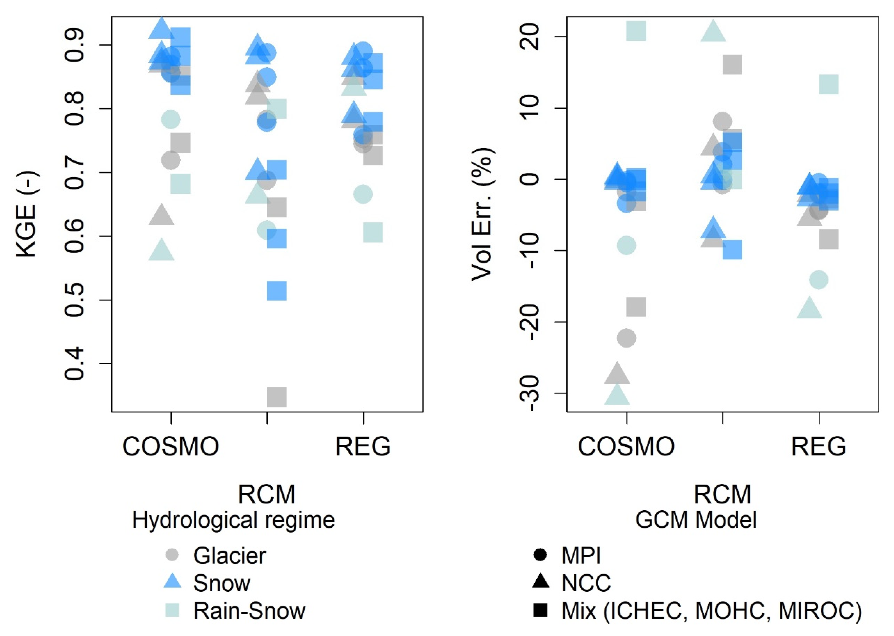
Figure 4. Kling–Gupta Efficiency (KGE; (left panel)) and runoff volume error (VE, %; (right panel)) for the nine CORDEX-SA members and six sub-basins in the calibration period 1981–1999. Marker colour indicates the hydroclimatic regime of the basin (dark blue: glacier-dominated; light blue: snow-dominated; cyan: rain–snow-mixed), and marker shape indicates the driving GCM group (circles: MPI; triangles: NCC; squares: mixed GCMs comprising EC-EARTH, HadGEM2-ES and MIROC5). Member identifiers (M1–M9) are as listed in Table 2.

Figure 4. Kling–Gupta Efficiency (KGE; (left panel)) and runoff volume error (VE, %; (right panel)) for the nine CORDEX-SA members and six sub-basins in the calibration period 1981–1999. Marker colour indicates the hydroclimatic regime of the basin (dark blue: glacier-dominated; light blue: snow-dominated; cyan: rain–snow-mixed), and marker shape indicates the driving GCM group (circles: MPI; triangles: NCC; squares: mixed GCMs comprising EC-EARTH, HadGEM2-ES and MIROC5). Member identifiers (M1–M9) are as listed in Table 2.

In the calibration period, model performance is strongly regime-dependent (Figure 4). Snow-dominated basins (Gilgit, Chitral, and Astore) are reproduced with the highest skill: KGE values typically fall between 0.70 and 0.92, and most members underestimate runoff volume by less than 10%. Glacier-dominated basins (Hunza and Shyok) show wider scatter, with KGE between 0.35 and 0.87 and runoff volumes that are mostly underestimated, particularly in Hunza (VE as low as −28%). The rain–snow-mixed basin (Swat) exhibits the largest spread, with KGE between 0.57 and 0.83 and volume errors ranging from approximately −30% to +20%.

Across the three RCMs, COSMO-crCLIM-v1-1 yields the highest mean KGE (0.82, range 0.66–0.91), followed closely by RegCM4-7 (0.80, range 0.57–0.92), while REMO2015 performs noticeably worse on average (0.72, range 0.35–0.89). The lower mean for REMO2015 is driven primarily by member M8 (HadGEM2-ES/REMO2015), which consistently underperforms in all basins (mean KGE 0.60). The remaining REMO members (M2, M5) produce KGE values in the same range as COSMO- and RegCM4-driven members. Differences across the driving GCM groups (MPI, NCC, mixed) are smaller than differences across RCMs.

Table 4. Kling–Gupta Efficiency (KGE; Equation (1)) for each sub-basin and CORDEX-SA member in the calibration period 1981–1999. The highest KGE in each basin is shown in bold.

ID	CORDEX-SA Member	Hunza	Shyok	Gilgit	Chitral	Astore	Swat
M1	MPI-ESM-LR/COSMO-crCLIM-v1-1	0.75	0.85	0.91	0.88	0.84	0.68
M2	MPI-ESM-LR/REMO2015	0.75	0.74	0.89	0.86	0.76	0.67
M3	MPI-ESM-MR/RegCM4-7	0.69	0.78	0.89	0.85	0.78	0.61
M4	NorESM1-M/COSMO-crCLIM-v1-1	0.85	0.78	0.86	0.88	0.79	0.83
M5	NorESM1-M/REMO2015	0.76	0.73	0.87	0.85	0.78	0.61
M6	NorESM1-M/RegCM4-7	0.72	0.86	0.87	0.88	0.86	0.78
M7	EC-EARTH/COSMO-crCLIM-v1-1	0.84	0.82	0.88	0.90	0.70	0.66
M8	HadGEM2-ES/REMO2015	0.65	0.35	0.51	0.70	0.60	0.80
M9	MIROC5/RegCM4-7	0.63	0.87	0.92	0.88	0.87	0.57

Table 4. Kling–Gupta Efficiency (KGE; Equation (1)) for each sub-basin and CORDEX-SA member in the calibration period 1981–1999. The highest KGE in each basin is shown in bold.

ID	CORDEX-SA Member	Hunza	Shyok	Gilgit	Chitral	Astore	Swat
M1	MPI-ESM-LR/COSMO-crCLIM-v1-1	0.75	0.85	0.91	0.88	0.84	0.68
M2	MPI-ESM-LR/REMO2015	0.75	0.74	0.89	0.86	0.76	0.67
M3	MPI-ESM-MR/RegCM4-7	0.69	0.78	0.89	0.85	0.78	0.61
M4	NorESM1-M/COSMO-crCLIM-v1-1	0.85	0.78	0.86	0.88	0.79	0.83
M5	NorESM1-M/REMO2015	0.76	0.73	0.87	0.85	0.78	0.61
M6	NorESM1-M/RegCM4-7	0.72	0.86	0.87	0.88	0.86	0.78
M7	EC-EARTH/COSMO-crCLIM-v1-1	0.84	0.82	0.88	0.90	0.70	0.66
M8	HadGEM2-ES/REMO2015	0.65	0.35	0.51	0.70	0.60	0.80
M9	MIROC5/RegCM4-7	0.63	0.87	0.92	0.88	0.87	0.57

Table 5. Runoff volume error (VE, %; Equation (2)) for each sub-basin and CORDEX-SA member in the calibration period 1981–1999. Negative values indicate underestimation, positive values overestimation.

ID	CORDEX-SA Member	Hunza	Shyok	Gilgit	Chitral	Astore	Swat
M1	MPI-ESM-LR/COSMO-crCLIM-v1-1	−17.9	−3.1	−0.2	−0.1	−1.7	−20.8
M2	MPI-ESM-LR/REMO2015	−2.7	−8.4	−1.2	−2.0	−3.0	−13.3
M3	MPI-ESM-MR/RegCM4-7	−5.5	−2.1	−1.1	−1.1	−2.7	−18.4
M4	NorESM1-M/COSMO-crCLIM-v1-1	−0.8	8.1	3.8	−0.1	2.1	−0.9
M5	NorESM1-M/REMO2015	−4.3	−4.4	−2.1	−1.9	−0.5	−14.1
M6	NorESM1-M/RegCM4-7	−22.3	−1.8	−3.4	−0.2	−0.5	−9.3
M7	EC-EARTH/COSMO-crCLIM-v1-1	−8.5	4.4	0.5	−0.4	−7.2	−20.4
M8	HadGEM2-ES/REMO2015	5.6	16.1	2.7	5.2	−9.9	0.0
M9	MIROC5/RegCM4-7	−27.6	−0.2	0.2	0.4	−0.4	−30.6

Table 5. Runoff volume error (VE, %; Equation (2)) for each sub-basin and CORDEX-SA member in the calibration period 1981–1999. Negative values indicate underestimation, positive values overestimation.

ID	CORDEX-SA Member	Hunza	Shyok	Gilgit	Chitral	Astore	Swat
M1	MPI-ESM-LR/COSMO-crCLIM-v1-1	−17.9	−3.1	−0.2	−0.1	−1.7	−20.8
M2	MPI-ESM-LR/REMO2015	−2.7	−8.4	−1.2	−2.0	−3.0	−13.3
M3	MPI-ESM-MR/RegCM4-7	−5.5	−2.1	−1.1	−1.1	−2.7	−18.4
M4	NorESM1-M/COSMO-crCLIM-v1-1	−0.8	8.1	3.8	−0.1	2.1	−0.9
M5	NorESM1-M/REMO2015	−4.3	−4.4	−2.1	−1.9	−0.5	−14.1
M6	NorESM1-M/RegCM4-7	−22.3	−1.8	−3.4	−0.2	−0.5	−9.3
M7	EC-EARTH/COSMO-crCLIM-v1-1	−8.5	4.4	0.5	−0.4	−7.2	−20.4
M8	HadGEM2-ES/REMO2015	5.6	16.1	2.7	5.2	−9.9	0.0
M9	MIROC5/RegCM4-7	−27.6	−0.2	0.2	0.4	−0.4	−30.6

Looking at individual basins (Table 4 and Table 5), the highest calibration KGE in Hunza is achieved by M4 (NorESM1-M/COSMO; 0.85), in Shyok and Astore by M9 (MIROC5/RegCM4-7; 0.87), in Gilgit again by M9 (0.92), in Chitral by M7 (EC-EARTH/COSMO; 0.90), and in Swat by M4 (0.83). The corresponding volume errors are generally small for the snow-dominated basins (|VE| ≤ 10% for most members in Gilgit, Chitral and Astore) but more variable in the glacier-dominated basins, where several members underestimate runoff by 17–28% in Hunza and in Swat, where errors range from approximately −30% to +20%.

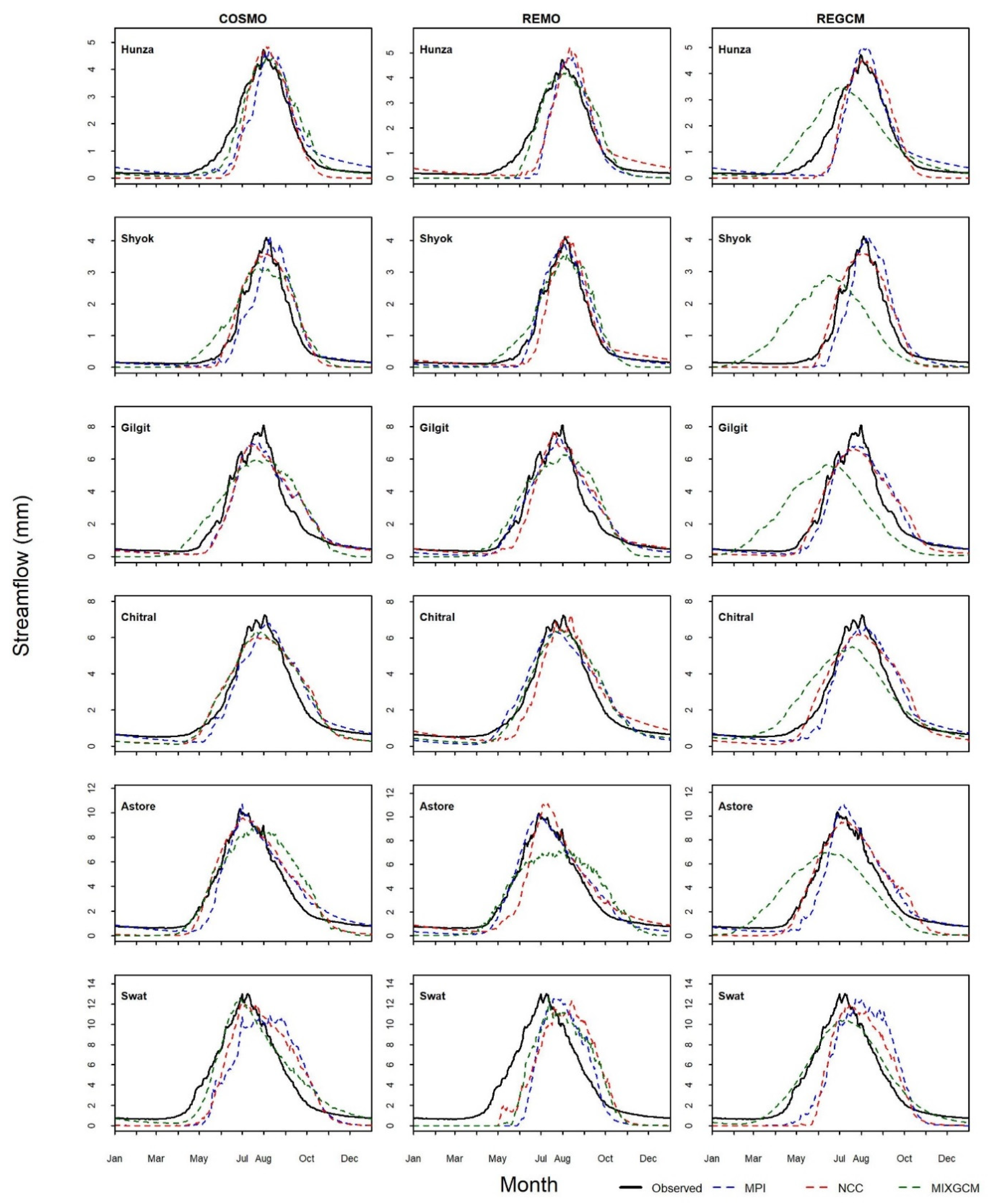
Figure 5. Mean monthly regime curves of observed (black) and CORDEX-SA-simulated (coloured) daily streamflow for the six sub-basins in the calibration period 1981–1999. Each coloured line shows the simulation driven by one of the nine CORDEX-SA members (M1–M9; Table 2).

Figure 5. Mean monthly regime curves of observed (black) and CORDEX-SA-simulated (coloured) daily streamflow for the six sub-basins in the calibration period 1981–1999. Each coloured line shows the simulation driven by one of the nine CORDEX-SA members (M1–M9; Table 2).

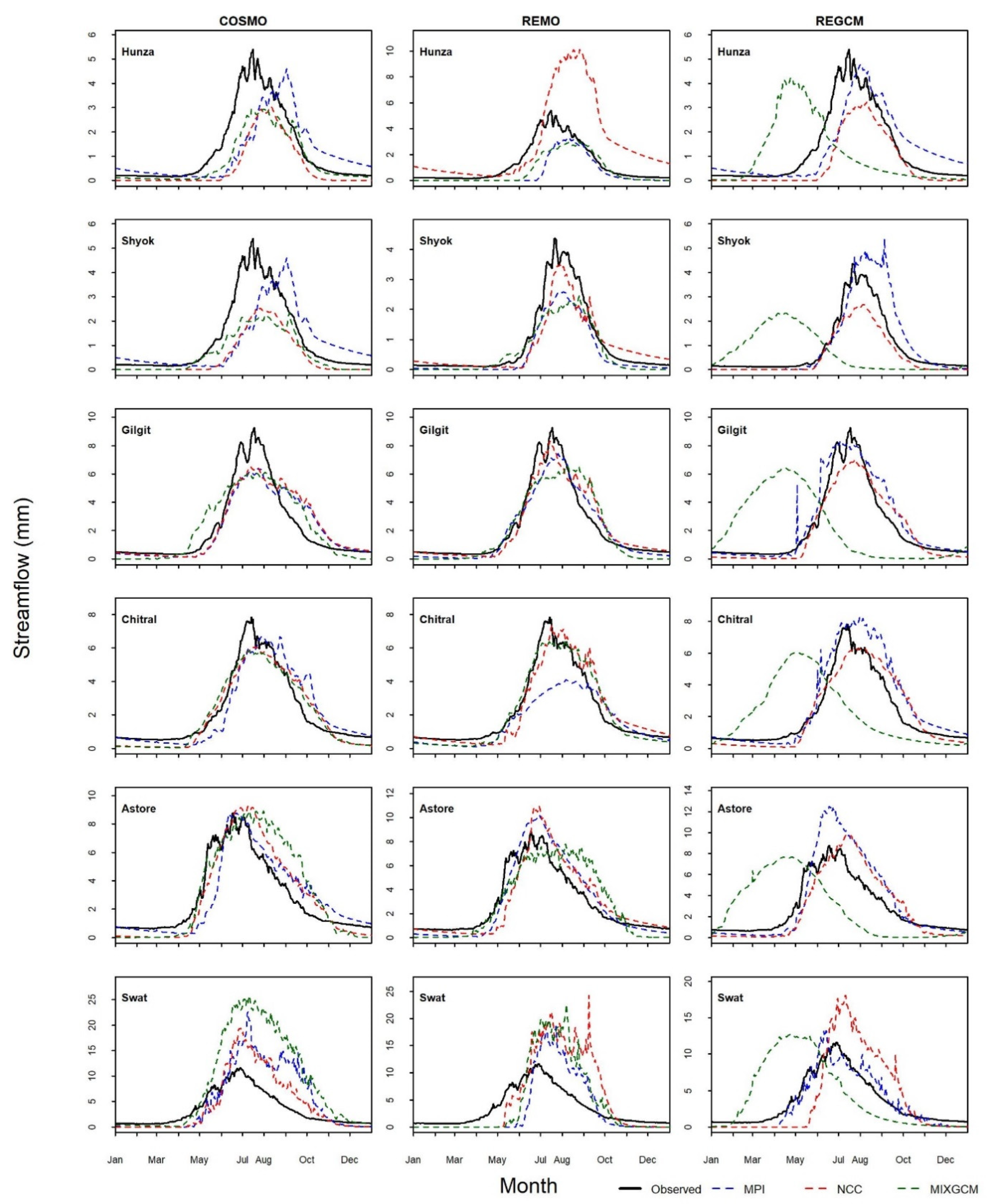
Figure 5 compares the mean monthly regime curves of observed and simulated streamflow during the calibration period. In the glacier-dominated basins (Hunza and Shyok), the observed peak occurs in July–August and is broadly reproduced by all members except M8 (HadGEM2-ES/REMO2015), which strongly underestimates the summer peak. In Hunza, several members underestimate the peak magnitude even when the timing is well-captured, consistent with the negative volume errors reported in Table 5. The snow-dominated basins (Gilgit, Chitral, and Astore) show an earlier, smoother rise driven by spring snowmelt. This pattern is reproduced consistently by most members, with the inter-member spread being smallest in Chitral. The rain–snow-mixed basin (Swat) exhibits the largest inter-member spread; members differ both in the timing and in the amplitude of the monsoon-influenced summer peak, with M3 (MPI-ESM-MR/RegCM4-7) underestimating and several other members overestimating it.

3.2. Performance in the Validation Period (2000–2005)

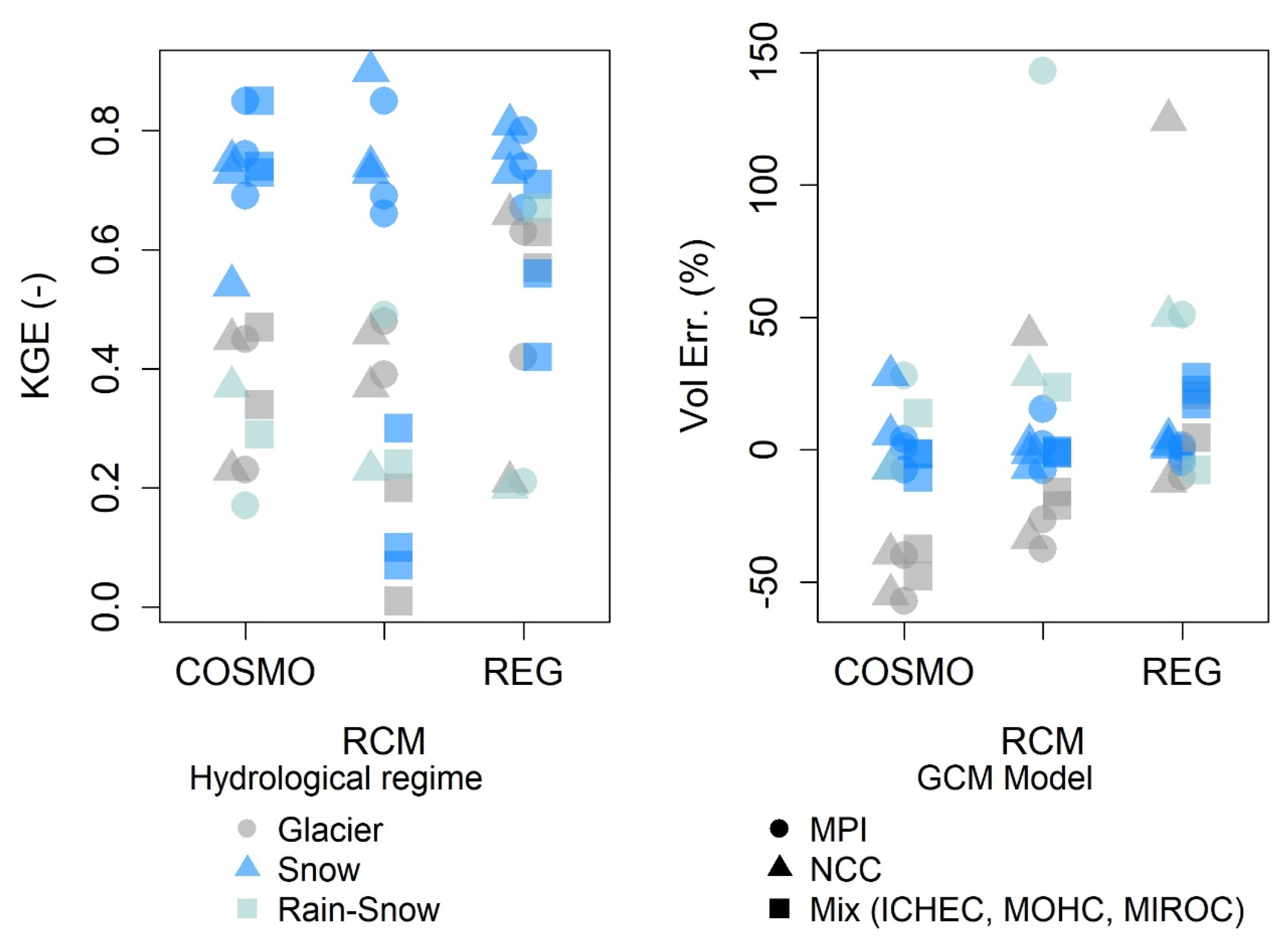
In the validation period (Figure 6), the regime-dependent pattern observed during calibration is preserved but with overall lower skill, as expected when transferring calibrated parameters to an independent period. Snow-dominated basins again perform best, with KGE values typically between 0.5 and 0.9 and the lowest inter-member spread. Glacier-dominated basins show substantially reduced KGE compared with calibration: median KGE drops from approximately 0.78 in calibration to 0.45 in validation in Hunza, and from 0.78 to 0.48 in Shyok. The rain–snow-mixed basin (Swat) is the most challenging during validation; several members produce negative KGE values, and only three of the nine members (M2, M5 and M9) achieve KGE > 0.3.

Figure 6. Kling–Gupta Efficiency (KGE; (left panel)) and runoff volume error (VE, %; (right panel)) for the nine CORDEX-SA members and six sub-basins in the validation period 2000–2005. Symbols and colours as in Figure 4.

Figure 6. Kling–Gupta Efficiency (KGE; (left panel)) and runoff volume error (VE, %; (right panel)) for the nine CORDEX-SA members and six sub-basins in the validation period 2000–2005. Symbols and colours as in Figure 4.

The mean validation KGE is highest for COSMO-crCLIM-v1-1 (0.48), followed closely by RegCM4-7 (0.47), with REMO2015 again the lowest (0.35). The relative ranking of RCMs is therefore consistent between calibration and validation, although the absolute differences between COSMO and RegCM4-7 are small. Volume errors are substantially larger in validation than in calibration, with several members showing |VE| > 40% in Hunza, Shyok and Swat (Table 7). Notably, the best calibrator is not always the best validator in the same basin.

Table 6. Kling–Gupta Efficiency (KGE; Equation (1)) for each sub-basin and CORDEX-SA member in the validation period 2000–2005. The highest KGE in each basin is shown in bold.

ID	CORDEX-SA Member	Hunza	Shyok	Gilgit	Chitral	Astore	Swat
M1	MPI-ESM-LR/COSMO-crCLIM-v1-1	0.34	0.47	0.74	0.85	0.73	0.29
M2	MPI-ESM-LR/REMO2015	0.63	0.57	0.71	0.56	0.42	0.67
M3	MPI-ESM-MR/RegCM4-7	−0.52	0.66	0.77	0.81	0.73	−0.26
M4	NorESM1-M/COSMO-crCLIM-v1-1	0.39	0.48	0.69	0.85	0.66	−1.08
M5	NorESM1-M/REMO2015	0.42	0.63	0.67	0.80	0.74	−0.12
M6	NorESM1-M/RegCM4-7	0.23	0.45	0.69	0.84	0.76	0.17
M7	EC-EARTH/COSMO-crCLIM-v1-1	0.37	0.46	0.73	0.90	0.74	−0.05
M8	HadGEM2-ES/REMO2015	−0.05	−0.44	−0.30	0.07	0.10	0.24
M9	MIROC5/RegCM4-7	0.23	0.45	0.75	0.54	0.73	0.37

Table 6. Kling–Gupta Efficiency (KGE; Equation (1)) for each sub-basin and CORDEX-SA member in the validation period 2000–2005. The highest KGE in each basin is shown in bold.

ID	CORDEX-SA Member	Hunza	Shyok	Gilgit	Chitral	Astore	Swat
M1	MPI-ESM-LR/COSMO-crCLIM-v1-1	0.34	0.47	0.74	0.85	0.73	0.29
M2	MPI-ESM-LR/REMO2015	0.63	0.57	0.71	0.56	0.42	0.67
M3	MPI-ESM-MR/RegCM4-7	−0.52	0.66	0.77	0.81	0.73	−0.26
M4	NorESM1-M/COSMO-crCLIM-v1-1	0.39	0.48	0.69	0.85	0.66	−1.08
M5	NorESM1-M/REMO2015	0.42	0.63	0.67	0.80	0.74	−0.12
M6	NorESM1-M/RegCM4-7	0.23	0.45	0.69	0.84	0.76	0.17
M7	EC-EARTH/COSMO-crCLIM-v1-1	0.37	0.46	0.73	0.90	0.74	−0.05
M8	HadGEM2-ES/REMO2015	−0.05	−0.44	−0.30	0.07	0.10	0.24
M9	MIROC5/RegCM4-7	0.23	0.45	0.75	0.54	0.73	0.37

Table 7. Runoff volume error (VE, %; Equation (2)) for each sub-basin and CORDEX-SA member in the validation period 2000–2005. Negative values indicate underestimation, positive values overestimation.

ID	CORDEX-SA Member	Hunza	Shyok	Gilgit	Chitral	Astore	Swat
M1	MPI-ESM-LR/COSMO-crCLIM-v1-1	−47.8	−37.6	−10.6	−1.8	−1.5	13.8
M2	MPI-ESM-LR/REMO2015	4.4	20.6	17.2	27.2	22.6	−7.7
M3	MPI-ESM-MR/RegCM4-7	124.4	−12.3	0.6	1.7	4.3	50.5
M4	NorESM1-M/COSMO-crCLIM-v1-1	−37.5	−26.4	1.9	−7.8	15.3	142.9
M5	NorESM1-M/REMO2015	−10.4	−3.2	−4.9	0.4	1.4	50.8
M6	NorESM1-M/RegCM4-7	−57.2	−40.0	1.0	−7.6	3.9	27.9
M7	EC-EARTH/COSMO-crCLIM-v1-1	−43.3	−33.4	−7.0	−1.3	2.0	28.2
M8	HadGEM2-ES/REMO2015	−16.1	−21.1	−1.5	−0.4	−1.1	23.5
M9	MIROC5/RegCM4-7	−54.7	−39.3	−7.3	−28.1	5.6	−7.1

Table 7. Runoff volume error (VE, %; Equation (2)) for each sub-basin and CORDEX-SA member in the validation period 2000–2005. Negative values indicate underestimation, positive values overestimation.

ID	CORDEX-SA Member	Hunza	Shyok	Gilgit	Chitral	Astore	Swat
M1	MPI-ESM-LR/COSMO-crCLIM-v1-1	−47.8	−37.6	−10.6	−1.8	−1.5	13.8
M2	MPI-ESM-LR/REMO2015	4.4	20.6	17.2	27.2	22.6	−7.7
M3	MPI-ESM-MR/RegCM4-7	124.4	−12.3	0.6	1.7	4.3	50.5
M4	NorESM1-M/COSMO-crCLIM-v1-1	−37.5	−26.4	1.9	−7.8	15.3	142.9
M5	NorESM1-M/REMO2015	−10.4	−3.2	−4.9	0.4	1.4	50.8
M6	NorESM1-M/RegCM4-7	−57.2	−40.0	1.0	−7.6	3.9	27.9
M7	EC-EARTH/COSMO-crCLIM-v1-1	−43.3	−33.4	−7.0	−1.3	2.0	28.2
M8	HadGEM2-ES/REMO2015	−16.1	−21.1	−1.5	−0.4	−1.1	23.5
M9	MIROC5/RegCM4-7	−54.7	−39.3	−7.3	−28.1	5.6	−7.1

The best validators per basin (Table 6) are M2 (MPI-ESM-LR/REMO2015) for Hunza (KGE = 0.63), M3 (MPI-ESM-MR/RegCM4-7) for Shyok (0.66) and Gilgit (0.77), M7 (EC-EARTH/COSMO) for Chitral (0.90), M6 (NorESM1-M/RegCM4-7) for Astore (0.76), and M2 again for Swat (0.67). Only in Chitral does the same member (M7) achieve the highest score in both calibration and validation. In the other five basins the best calibrator differs from the best validator, although the differences in KGE among the top three members in each basin are typically small (within 0.05–0.10).

Figure 7. Mean monthly regime curves of observed (black) and CORDEX-SA-simulated (coloured) daily streamflow for the six sub-basins in the validation period 2000–2005. Each coloured line shows the simulation driven by one of the nine CORDEX-SA members (M1–M9; Table 2).

Figure 7. Mean monthly regime curves of observed (black) and CORDEX-SA-simulated (coloured) daily streamflow for the six sub-basins in the validation period 2000–2005. Each coloured line shows the simulation driven by one of the nine CORDEX-SA members (M1–M9; Table 2).

In the validation period (Figure 7), the simulated regime curves for the glacier-dominated basins (Hunza and Shyok) deviate more clearly from the observed hydrographs than in calibration. In Hunza, most members underestimate the summer peak by 20–50%, with M3 being a notable outlier that strongly overestimates summer flow (consistent with VE = +124% in Table 7). In Shyok, the inter-member range is more balanced, but most members still underestimate the peak. The snow-dominated basins reproduce both the timing and magnitude of the seasonal cycle more reliably; Chitral, in particular, shows close agreement between most members and the observed hydrograph. In the rain–snow-mixed basin (Swat), the spread is largest, with some members (notably M4, M3, and M6) substantially overestimating peak flow during the validation period.

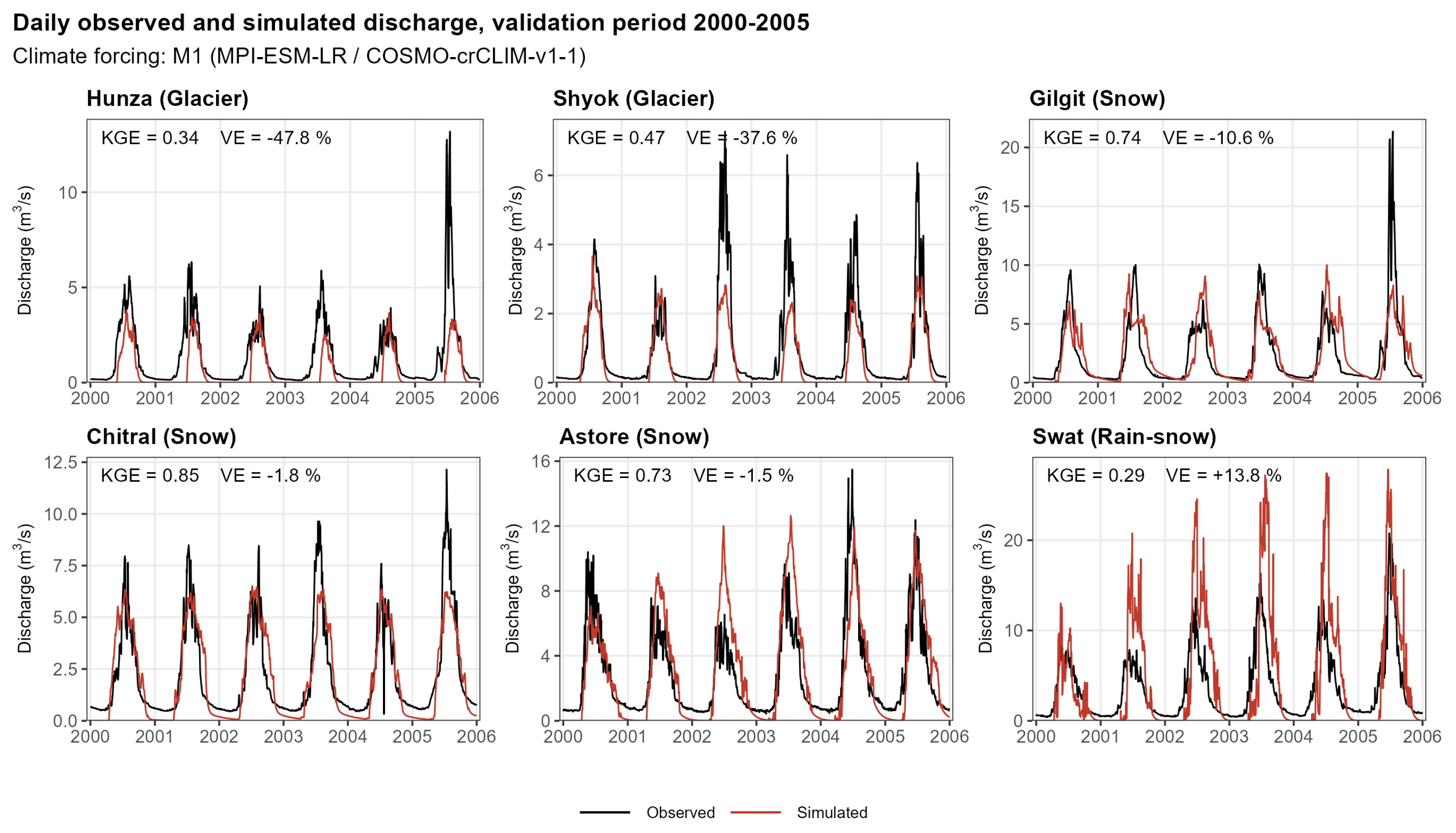
Figure 8 shows the daily simulated and observed hydrographs for the validation period using member M1 (MPI-ESM-LR/COSMO-crCLIM-v1-1), which was selected as a representative ensemble member because it produces the most consistent skill across basins and across periods (mean rank 3.6 of 9 across the 12 basin–period combinations). The figure illustrates the regime-dependent skill discussed above at daily resolution: in the snow-dominated basins (Gilgit, Chitral, and Astore), the simulated hydrograph closely follows the observed seasonal rise, recession and inter-annual variability of the snowmelt peak; in the glacier-dominated basins (Hunzaand Shyok), the timing of the summer melt pulse is captured but the daily peak magnitudes are systematically underestimated; and in the rain–snow-mixed basin (Swat) the simulated discharge fails to reproduce the short, intense monsoon-driven peaks of 2001–2003 and 2005. Daily hydrographs for the remaining eight CORDEX-SA members are provided in the Supplementary Material (Figures S3–S10).

The corresponding climatology of forcing variables and simulated discharge for the validation period is shown in Supplementary Figure S9 (monthly climatology of precipitation, near-surface air temperature and simulated discharge for the six sub-basins during the validation period 2000–2005, grouped by hydroclimatic regime; layout as in Figure 3).

3.3. Extreme-Flow Performance

Beyond the aggregated performance metrics, the high- and low-flow signatures (

Table 8. High- and low-flow signatures by sub-basin (median (min, max) of nine members). FHV = high-flow-volume bias (top 2% of flows); Q_max bias = percent bias in the annual-maximum daily discharge; Q95 = percent bias in the flow exceeded 95% of the time (low flow); peak timing = median absolute error in the date of the annual maximum (days). Positive = overestimation.

Sub-Basin	Period	FHV (%)	Qmax Bias (%)	Q95 (%)	Peak Timing (d)
Hunza	Calibration	−3.8 [−22, +16]	+2.2 [−24, +5]	−78.8 [−100, −43]	16.2
	Validation	−50.7 [−62, +25]	−37.9 [−49, +72]	−91.8 [−100, +169]	19.3
Shyok	Calibration	−20.4 [−31, +8]	−12.6 [−33, +4]	−99.7 [−100, −85]	14.8
	Validation	−51.7 [−54, +14]	−42.4 [−52, +34]	−99.8 [−100, −51]	19.7
Gilgit	Calibration	−14.1 [−29, −2]	−4.7 [−26, +5]	−80.5 [−100, −56]	16.4
	Validation	−44.0 [−54, −25]	−22.1 [−40, +25]	−81.4 [−100, −47]	24.3
Chitral	Calibration	−14.1 [−21, +5]	−19.6 [−26, +4]	−74.6 [−89, −51]	17.4
	Validation	−21.0 [−35, +15]	−23.9 [−43, +27]	−80.5 [−93, −53]	18.0
Astore	Calibration	−19.8 [−48, +4]	−23.2 [−46, −3]	−97.1 [−100, −35]	20.4
	Validation	−6.8 [−34, +27]	+3.5 [−22, +48]	−89.6 [−100, −51]	21.3
Swat	Calibration	−7.2 [−26, +21]	−2.8 [−28, +14]	−100.0 [−100, −70]	24.5
	Validation	+51.3 [−11, +88]	+85.4 [+6, +182]	−100.0 [−100, −65]	33.3

) indicate three distinct regime-dependent behaviours. All values are reported as the median together with the inter-member range across the nine ensemble members, consistent with the range-based representation of efficiency metrics; the median is adopted due to the pronounced right-skewness of the extreme-flow distributions.

In glacier-dominated basins (Hunza, Shyok), high-flow volumes are reproduced reasonably well during calibration (median FHV ≈ −11%) but are substantially underestimated in the validation period (median FHV ≈ −51%, with an inter-member range of −62% to +25%; median annual-maximum bias ≈ −42%). While the timing of peak flows is captured within approximately 25–29 days, their magnitude is consistently under-simulated, indicating insufficient representation of melt-season runoff under the uncorrected forcing.

Snow-dominated basins (Gilgit, Chitral, Astore) exhibit more moderate and temporally stable peak-flow biases (median validation FHV ≈ −25%, with Astore showing near-neutral bias), consistent with their comparatively higher overall model performance.

In contrast, the rain–snow-dominated Swat basin shows pronounced overestimation and strong inter-member variability in validation (median FHV +51% and median annual-maximum bias +85%, with ranges of −11% to +88% and +6% to +182%, respectively), suggesting that the 0.22° forcing is unable to consistently resolve the sub-grid-scale convective precipitation events that govern peak runoff generation.

Low flows are systematically underestimated across all basins and both periods, with median Q90 and Q95 biases typically ranging from approximately −76% to −100% (with 92% of all basin–member–period combinations underestimating Q95 by more than 50%). This pervasive depletion of simulated baseflow, which is not evident from hydrograph inspection alone, reflects a structural limitation of the conceptual model under uncorrected forcing and also explains why the logarithmic FLV signature proved uninformative in this context. While this limitation is relevant for low-flow and drought applications, it does not affect the primary conclusions of this study, which focus on overall performance, high-flow behaviour, and its regime dependence.

Partition of KGE (

Table 9. KGE and its components by sub-basin (median of nine members). KGE partitioned into correlation (r, timing), variability ratio (α) and bias ratio (β); NSE for reference. α < 1 and β < 1 indicate under-simulation of variability and volume; α > 1 and β > 1 indicate over-simulation.

Sub-Basin	Period	KGE	r	α	β	NSE
Hunza	Calibration	0.75	0.76	1.03	0.94	0.52
	Validation	0.36	0.68	0.62	0.63	0.32
Shyok	Calibration	0.78	0.81	1.00	0.98	0.63
	Validation	0.46	0.78	0.64	0.74	0.60
Gilgit	Calibration	0.88	0.88	1.00	1.00	0.76
	Validation	0.70	0.77	0.81	0.98	0.58
Chitral	Calibration	0.88	0.88	1.01	1.00	0.76
	Validation	0.80	0.84	1.00	1.00	0.60
Astore	Calibration	0.78	0.78	1.02	0.98	0.58
	Validation	0.73	0.79	1.17	1.05	0.47
Swat	Calibration	0.67	0.73	1.07	0.86	0.41
	Validation	0.16	0.71	1.76	1.29	−0.87

) provides further insight into the underlying sources of model performance. In the snow-dominated basins, validation performance is constrained primarily by the correlation component, with a median r of approximately 0.80, whereas the variability and bias ratios remain close to unity (α ≈ 1.0, β ≈ 1.0), indicating minimal systematic errors in flow variability and volume. In contrast, the glacier-dominated basins exhibit substantially reduced variability and bias ratios during validation (α ≈ 0.64, β ≈ 0.70), together with a lower correlation (r ≈ 0.73), confirming a systematic underestimation of melt-season streamflow. In the rain–snow basin, although the correlation remains comparable (r ≈ 0.71), both the variability and bias ratios exceed unity (α ≈ 1.76, β ≈ 1.29). This indicates that the marked decline in KGE is primarily attributable to an excessive hydrological response to monsoon precipitation rather than deficiencies in flow timing.

Analysis by driving RCM (

Table 10. Performance grouped by driving RCM (median of all basins). COSMO = M1, M4, M7; REMO = M2, M5, M8; RegCM4 = M3, M6, M9 (Table 2). This mirrors the RCM grouping used for the efficiency metrics and tests whether the calibration-period COSMO advantage extends to the extremes.

RCM	Period	KGE	FHV (%)	Qmax Bias (%)	Q95 (%)
COSMO	Calibration	0.84	−5.7	−1.8	−87.8
	Validation	0.60	−26.7	−12.7	−88.3
REMO	Calibration	0.76	−18.0	−17.6	−87.6
	Validation	0.38	−28.4	−21.1	−90.0
RegCM4	Calibration	0.83	−14.2	−9.6	−99.6
	Validation	0.59	−26.8	−11.1	−99.6

) indicates that the calibration-period advantage of COSMO-crCLIM-v1-1 does not consistently translate to the simulation of flow extremes. During calibration, COSMO more accurately reproduces high flows, with a median FHV of −6%, compared with −18% for REMO2015 and −14% for RegCM4-7. However, this advantage disappears during validation, where all three RCMs exhibit similar performance (median FHV ≈ −27%), suggesting limited out-of-sample robustness. Moreover, in the rain–snow basin the relative ranking reverses, with COSMO producing the largest overestimation of monsoon peak flows; notably, the EC-EARTH/COSMO member M7 overestimates the annual maximum discharge by 182%. For low flows, all three RCMs perform similarly (median Q95 ranging from approximately −88% to −100%), indicating that the persistent underestimation of low flows is an inherent limitation of the hydrological model rather than a consequence of the meteorological forcing. Overall, these findings support and further refine the manuscript’s conclusion that the optimal climate model forcing varies among basin types.

4. Discussion

In this study, the conceptual snow–glacier hydrological model HBV-IANIGLA was calibrated and validated using daily precipitation and air temperature outputs from nine uncorrected CORDEX-SA members in six UIB sub-basins representing three contrasting hydroclimatic regimes. The discussion below addresses (i) the regime dependence of model performance; (ii) the relative roles of the GCM and the RCM; (iii) the stability of model ranking between calibration and validation; (iv) the implications for the use of bias correction; (v) the consistency of our results with the recent UIB literature; and (vi) the main limitations and directions for further work.

4.1. Regime-Dependent Performance

The central finding of this study is that the performance of uncorrected CORDEX-SA outputs as hydrological forcing in the UIB is strongly regime-dependent. Snow-dominated basins (Gilgit, Chitral, and Astore) are reproduced best, with mean ensemble KGE values of 0.83 in calibration and 0.64 in validation. Glacier-dominated basins (Hunzaand Shyok) are reproduced reasonably well in calibration (mean KGE 0.75) but show a marked drop in validation (mean KGE 0.32), while the rain–snow-mixed basin (Swat) is the most challenging, with most members losing skill in the validation period.

This regime gradient reflects the different hydrological processes that control runoff generation. In the snow-dominated basins, daily and seasonal streamflow is largely shaped by the temperature-driven progression of snowmelt, which is represented adequately by CORDEX-SA even without bias correction. In glacier-dominated basins, runoff additionally depends on ice melt and on the air temperature regime above 4 000 m, where CORDEX-SA grid cells coincide with sparse observational coverage. Small biases in high-elevation air temperature or in winter precipitation propagate into substantial errors in simulated summer melt [7,9,10]. In the rain–snow-mixed basin (Swat), the largest part of the annual flow originates from monsoon rainfall, whose intensity, timing and spatial distribution are known to be difficult to reproduce at the 0.22° resolution of the CORDEX-SA RCMs [14]. The contrast between snow-, glacier- and rain-driven regimes therefore explains most of the inter-basin variability observed in our results.

4.2. Inter-Model Variability and the Role of the RCM

Within the ensemble, the choice of RCM accounts for a larger share of the inter-model variability than the choice of driving GCM. On average, COSMO-crCLIM-v1-1 (mean KGE 0.82 in calibration and 0.48 in validation) and RegCM4-7 (0.80 and 0.47) perform comparably, and both outperform REMO2015 (0.72 and 0.35). This pattern is consistent with previous CORDEX evaluations that report substantial inter-RCM spread in simulated precipitation and air temperature even when the same driving GCM is used [50,51,52,53,54,55,56,57,58,59,60,61,62,63,64]. Because the hydrological response in cryosphere-influenced catchments is highly sensitive to the timing and magnitude of solid precipitation and to near-surface temperature thresholds, mismatches in these variables propagate directly into simulated snowfall, snowmelt and runoff [65,66]. The UIB amplifies this sensitivity because of its sparse high-altitude observational network [18,19].

One member of the ensemble, M8 (MOHC-HadGEM2-ES/REMO2015), performs markedly worse than all others across both periods and all basins, with mean KGE values of 0.60 in calibration and 0.13 in validation, and negative KGE in three basins during validation. The poor performance of this member is consistent across regimes, suggesting it reflects a structural issue with the HadGEM2-ES–REMO2015 pairing rather than a single-basin failure. This behaviour should be considered when interpreting ensemble-based applications of CORDEX-SA in the UIB.

A comparison between the M8 forcing and the remaining eight ensemble members provides a clear explanation for this behaviour. On average across all basins, M8 is approximately 6 °C colder than the other members and exhibits a pronounced wet bias, with annual precipitation higher by about 40–55% and monsoon-season (June–September) precipitation exceeding twice that of the ensemble mean. This combination of cold and wet conditions suppresses snow and glacier melt, as a larger fraction of precipitation is stored as snow rather than contributing to immediate runoff, thereby explaining the underestimated summer flows and the strongly negative validation KGE values in glacier- and snow-dominated basins, including values as low as −0.44 in Shyok. Conversely, the excessive monsoon precipitation enhances runoff generation during the warm season, leading to substantial overestimation of peak flows in the rain–snow-mixed Swat basin. As a result, M8 behaves as a clear outlier at both low- and high-flow extremes, and its inclusion may introduce significant bias in hydrological applications of CORDEX-SA for the Upper Indus Basin. Therefore, its exclusion or strong down-weighting is recommended, although this suggestion should be interpreted as specific to the present study region and modelling framework.

4.3. Stability of Model Ranking Between Calibration and Validation

A methodologically important observation is that the ranking of CORDEX-SA members is not stable between the calibration and validation periods. The highest-KGE member in calibration coincides with the highest-KGE member in validation in only one of the six basins (Chitral, where M7 is best in both periods). In the other five basins, the best calibrator and the best validator differ, although the differences among the top three members are typically small (within 0.05–0.10 in KGE). This rank instability has two main causes. First, the validation window (2000–2005) is short, six years compared with nineteen years for calibration, which makes the validation skill more sensitive to the specific hydroclimatic events of that period. Second, the relative ability of an RCM to reproduce the observed flow at daily resolution depends on year-to-year features of the climate forcing (for example, the timing of major monsoon pulses or anomalous melt seasons) that the model is not constrained to reproduce. The practical implication is that ensemble-based interpretation is more robust than single-best-member selection and that recommendations on which CORDEX-SA members to use for impact studies should be based on consistent performance across both periods (for example, M1, M7 and M6, which rank in the top three in several basins across both periods) rather than on the maximum KGE in a single period.

4.4. Extreme-Flow Behaviour Across Hydroclimatic Regimes

The performance of uncorrected CORDEX-SA forcing in simulating discharge extremes reveals clear hydrological regime-dependent limitations across the Upper Indus Basin. Glacier-dominated catchments (Hunza and Shyok) consistently underestimate melt-season peak flows, with biases becoming more pronounced during the validation period, suggesting that cold temperature biases and the underrepresentation of high-altitude snowfall reduce simulated glacier melt and summer runoff. Although snow-dominated basins exhibit comparatively smaller errors in peak discharge, the persistent and substantial underestimation of low flows indicates deficiencies in representing winter precipitation, groundwater contributions, and delayed snowmelt processes that sustain baseflow in high-altitude mountainous environments. In contrast, the rain–snow-mixed Swat basin shows considerable overestimation of peak flows during validation, highlighting the inability of uncorrected CORDEX-SA precipitation to adequately capture the intensity and timing of monsoon rainfall. Furthermore, the systematic delay in simulated peak discharge across all catchments suggests that the timing of snow accumulation, melt, and precipitation processes is not fully represented by the climate forcing.

4.5. Parameter Variability and Equifinality

The 54 calibrated parameter sets (nine forcing members across six sub-basins) were evaluated as an ensemble of optimal solutions. Across the nine forcing members, the calibrated parameters exhibit substantial variability, with most of the 22 parameters showing relative ranges exceeding 0.7 of their respective prior intervals (Table S2). This indicates that, under uncorrected forcing, the calibration does not converge towards a single unique parameterisation; instead, parameter adjustment compensates for systematic differences among forcing members. Despite this overall spread, a clear hierarchy in parameter identifiability is evident. The routing recession constants (K1 and K2; median relative ranges of 0.32 and 0.24, respectively) and the snowmelt factor (fm_snow; 0.48) are comparatively better constrained, as they primarily govern flow recession behaviour and total melt contribution. In contrast, parameters controlling melt thresholds (Tt_snow and Tt_ice; ≈1.0), the unit hydrograph base (Bmax; ≈1.0), soil water storage capacity (FC; 0.98), and soil-moisture threshold (LP; 0.93) remain effectively unconstrained, reflecting weak sensitivity to model performance. Consistent with this, the routing module shows the highest degree of identifiability (0.50), whereas the transfer and soil modules are least constrained (1.00 and 0.94, respectively).

Importantly, parameter identifiability does not improve in glacier-dominated basins (Hunza and Shyok), where the median relative range (0.82) is comparable to that of the remaining basins (0.84). This suggests that even in cryosphere-dominated catchments, glacier-related parameters are not independently identifiable and instead compensate for interactions among snow and soil processes. The correlation structure further supports this compensatory behaviour, with the strongest dependencies observed between the ice melt factor and glacier recession parameter (fm_ice–KGmin; ρ = 0.80), between the two routing recession parameters (K1–K2; ρ = 0.75), and between soil storage and evapotranspiration threshold parameters (FC–LP; ρ = −0.50). Collectively, the wide parameter ranges across forcing members and the presence of strong inter-parameter dependencies provide a clear empirical manifestation of equifinality, demonstrating that calibration primarily absorbs discrepancies arising from differences in forcing rather than identifying physically unique parameter values.

It is emphasised that this analysis describes parameter variability within a calibrated ensemble as an indicator of identifiability and equifinality, rather than constituting a full probabilistic uncertainty assessment. Such an analysis is constrained by the relatively short observational record (1981–2005) and is therefore identified as a defined next step (Section 4.8).

4.6. Bias Correction Trade-Offs

Our results show that, for snow-dominated basins, a subset of uncorrected CORDEX-SA members already reproduces observed streamflow with skill comparable to that achieved by bias-corrected forcing in other UIB studies [9,26]. Bias correction is widely used to align RCM outputs with observations, but several studies have documented that bias-correction methods can distort the underlying climate change signal, alter non-stationary features of the climate, and introduce new uncertainties into the simulated discharge [34,35,36,67,68]. The trade-off is therefore not between bias correction and no correction in absolute terms, but rather the relative weight of two error sources: residual climate biases in the uncorrected forcing on the one hand, and post-correction distortion of the climate signal on the other. In data-scarce mountainous regions like the UIB, where bias correction relies on observations of limited spatial coverage and quality, the second source can be substantial. The present results suggest that, at least for snow-dominated catchments, uncorrected CORDEX-SA forcing is a defensible alternative to bias-corrected forcing, while for glacier-dominated and monsoon-influenced catchments, bias correction used with caution and with explicit evaluation of its effect on the climate signal is likely to remain necessary.

When bias correction is implemented, selecting an appropriate method is critical. For monsoon precipitation, distribution-based, trend-preserving approaches such as quantile delta mapping are recommended, as they adjust the full distribution of values while retaining the underlying climate change signal. In contrast, simple linear scaling is insufficient for representing extremes that strongly influence glacier- and monsoon-driven runoff. For high-altitude temperature, variance-preserving (scaled distribution) methods are more suitable, while in cases where consistency between precipitation and temperature is required, multivariate, trend-preserving techniques such as MBCn should be preferred. Quantitatively, bias correction in glacier- and monsoon-influenced basins should aim to reduce the large validation volume errors observed here (approximately −57% to +143%) towards the ±10–15% range already achieved in snow-dominated basins using uncorrected forcing, while ensuring that the timing component of model performance (as reflected in KGE correlation) is not degraded. However, the effectiveness of any bias correction approach in the Upper Indus Basin remains fundamentally constrained by the limited availability of high-altitude observational data.

4.7. Comparison with Previous UIB Studies

Our findings are broadly consistent with recent assessments of the UIB but extend them in two ways. Process-based modelling at high spatial resolution has shown that snowmelt is the dominant runoff component (about 54% of annual flow) and that glacier melt contributes about 11%, with the remainder coming from rainfall and baseflow [10]; these proportions are consistent with our finding that snow-dominated basins are the easiest to simulate from CORDEX-SA forcing, because the daily snowmelt response depends primarily on the air temperature signal, which RCMs reproduce relatively well. Bias-corrected CORDEX projections have indicated that high-altitude warming will shift the timing of snowmelt and reduce summer flows [7,9,14,26]; the regime-dependent skill we report supports the interpretation of those projections in snow-dominated basins but suggests greater caution in interpreting them for glacier- and monsoon-influenced sub-basins. Recent glacier-runoff projections suggest that the relative contribution of glaciers will evolve non-monotonically over the twenty-first century, with large Karakoram glaciers sustaining runoff longer than smaller ones [25]. This means that the volume errors we report for Hunza and Shyok using uncorrected forcing are likely to remain a concern for impact assessments in the coming decades and that improved representation of high-altitude air temperature and precipitation will be central to reducing these errors.

4.8. Limitations and Outlook

Several limitations of this study should be noted. First, the analysis is based on nine CORDEX-SA members; although this ensemble captures a representative range of inter-model variability for the South Asia domain, including additional RCMs (for example, from CORDEX-CORE) or larger initial-condition ensembles would strengthen the assessment of uncertainty. Second, the validation period (2000–2005) is short relative to the calibration period and is sensitive to a small number of hydroclimatic events; an extension to a longer evaluation window, or the use of moving cross-validation, would help to distinguish stable from event-specific aspects of model performance. Third, this study uses uncorrected forcing by design; a follow-up direct comparison with bias-corrected outputs from the same ensemble would quantify how much of the residual error is attributable to climate biases versus the limitations of the conceptual hydrological model.

A further limitation arises from the behaviour of the calibrated model parameters. Across the nine ensemble members, most parameters span nearly their full permissible calibration ranges, indicating weak identifiability. In practical terms, the observational data are insufficient to uniquely constrain parameter values, and multiple parameter combinations are able to reproduce observed streamflow with comparable performance. This phenomenon reflects equifinality, where different parameter sets yield similarly acceptable model outputs. Within this framework, only a limited number of parameters are well constrained, primarily the storage–recession constants governing drainage dynamics (K1 and K2) and, to a lesser extent, the snowmelt factor. In contrast, parameters associated with snow, glacier, and soil processes remain largely unconstrained, as substantial variation in their values produces negligible changes in model performance; consequently, their calibrated estimates should not be interpreted as physically unique or definitive.

These findings are further supported by complementary diagnostic analyses. The variance-based Sobol sensitivity analysis indicates that model skill is dominated by the upper-zone recession constant K1, with a secondary contribution from its interaction with K2, while snow-, glacier-, and soil-related parameters exert minimal influence on overall performance. This aligns with the observed inability to constrain these parameters during calibration. Similarly, the GLUE-based predictive uncertainty analysis shows that the ensemble spread generated by varying parameter sets is small relative to the residual mismatch between simulations and observations, implying that the dominant sources of error are structural rather than parametric in nature. In other words, the discrepancies arise primarily from model formulation and input forcing rather than from suboptimal parameter selection and therefore cannot be substantially reduced through further calibration alone. A full probabilistic uncertainty framework was not implemented due to limitations imposed by the short observational record (1981–2005), which restricts the feasibility of extensive re-calibration experiments; this remains an important avenue for future work.

Finally, the temporal robustness of model performance was assessed by calculating annual KGE values over the validation period. The overall regime ranking (snow-dominated basins performing best, followed by glacier-dominated, and then rain–snow systems) is preserved in five out of six years, indicating stable inter-catchment behaviour over time. Snow- and glacier-dominated basins maintain consistent skill across all years, demonstrating robustness of model performance in cryosphere-dominated regimes. In contrast, the rain–snow-mixed Swat basin exhibits pronounced interannual variability, with annual KGE values ranging from approximately −0.66 to +0.62, making it the principal source of temporal uncertainty. This behaviour is consistent with its high sensitivity to monsoon precipitation variability and associated forcing uncertainties.

Despite these limitations, the present results indicate that no single CORDEX-SA member performs uniformly best across all hydroclimatic regimes of the UIB and that the selection of climate forcing for hydrological modelling should be guided by the dominant runoff-generating processes of the catchment rather than by a single global ranking of RCMs.

5. Conclusions

This study assessed the performance of nine uncorrected CORDEX-SA GCM–RCM combinations as hydrological forcing in six sub-basins of the Upper Indus Basin (UIB), representing glacier-dominated (Hunza and Shyok), snow-dominated (Gilgit, Chitral, and Astore) and rain–snow-mixed (Swat) hydroclimatic regimes. The conceptual snow–glacier model HBV-IANIGLA was calibrated for 1981–1999 and validated for 2000–2005 using daily precipitation and temperature outputs from CORDEX-SA, without applying any bias correction to the climate data.

The results show that model skill is strongly regime-dependent. Snow-dominated basins are reproduced best (mean ensemble Kling–Gupta Efficiency of 0.83 in calibration and 0.64 in validation, with a maximum of 0.92), glacier-dominated basins are reproduced moderately well in calibration but with reduced skill in validation, and the rain–snow-mixed basin is the most challenging to simulate. Averaged across all basins, the COSMO-crCLIM-v1-1 and RegCM4-7 RCMs perform comparably, with both outperforming REMO2015. The best-performing CORDEX-SA member differs between basins and between the calibration and validation periods, indicating that hydrological assessment in the UIB benefits more from ensemble-based interpretation than from the selection of a single best member.

The practical implication is that, for snow-dominated catchments, carefully selected uncorrected CORDEX-SA outputs can support hydrological assessment in data-scarce high-mountain regions and provide a defensible alternative to bias-corrected forcing data. For glacier-dominated and monsoon-influenced catchments, additional treatment of climate forcing remains necessary because of larger residual biases in high-altitude temperatures and in monsoon precipitation. These findings provide guidance for the use of CORDEX-SA in climate-impact studies in the UIB and in other similar high-mountain basins.

References

1. Nie, Y.; Pritchard, H.D.; Liu, Q.; Hennig, T.; Wang, W.; Wang, X.; Liu, S.; Nepal, S.; Samyn, D.; Hewitt, K.; et al. Glacial change and hydrological implications in the Himalaya and Karakoram. Nat. Rev. Earth Environ. 2021, 2, 91–106. [Google Scholar] [CrossRef]
2. Pomee, M.S.; Hertig, E. Precipitation projections over the Indus River Basin of Pakistan for the 21st century using a statistical downscaling framework. Int. J. Climatol. 2022, 42, 289–314. [Google Scholar] [CrossRef]
3. Soncini, A.; Bocchiola, D.; Confortola, G.; Bianchi, A.; Rosso, R.; Mayer, C.; Lambrecht, A.; Palazzi, E.; Smiraglia, C.; Diolaiuti, G. Future hydrological regimes in the Upper Indus Basin: A case study from a high-altitude glacierized catchment. J. Hydrometeorol. 2015, 16, 306–326. [Google Scholar] [CrossRef]
4. Gertler, C.G.; Puppala, S.P.; Panday, A.; Stumm, D.; Shea, J. Black carbon and the Himalayan cryosphere: A review. Atmos. Environ. 2016, 125, 404–417. [Google Scholar] [CrossRef]
5. Immerzeel, W.W.; Van Beek, L.P.; Bierkens, M.F. Climate change will affect the Asian water towers. Science 2010, 328, 1382–1385. [Google Scholar] [CrossRef] [PubMed]
6. Krakauer, N.Y.; Lakhankar, T.; Dars, G.H. Precipitation trends over the Indus basin. Climate 2019, 7, 116. [Google Scholar] [CrossRef]
7. Lutz, A.F.; Immerzeel, W.W.; Kraaijenbrink, P.D.A.; Shrestha, A.B.; Bierkens, M.F.P. Climate change impacts on the Upper Indus hydrology: Sources, shifts and extremes. PLoS ONE 2016, 11, e0165630. [Google Scholar] [CrossRef] [PubMed]
8. Mukhopadhyay, B.; Khan, A. A reevaluation of the snowmelt and glacial melt in river flows within Upper Indus Basin and its significance in a changing climate. J. Hydrol. 2015, 527, 119–132. [Google Scholar] [CrossRef]
9. Shafeeque, M.; Luo, Y.; Arshad, A.; Muhammad, S.; Ashraf, M.; Pham, Q.B. Assessment of climate change impacts on glacio-hydrological processes and their variations within critical zone. Nat. Hazards 2022, 115, 2721–2748. [Google Scholar] [CrossRef]
10. Umer, M.; Wang, T.; Yang, D.; Liao, Z.; Aletoum, E.; Tang, L.; Li, P. Long-term hydrological dynamics and water balance in the Upper Indus Basin: Insights from a process-based model. J. Hydrol. Reg. Stud. 2026, 64, 103259. [Google Scholar] [CrossRef]
11. Mahessar, A.A.; Qureshi, A.L.; Dars, G.H.; Solangi, M.A. Climate change impacts on vulnerable Guddu and Sukkur barrages in Indus River, Sindh. Sindh Univ. Res. J. 2017, 49, 1. [Google Scholar]
12. Neupane, S.; Shrestha, S.; Ghimire, U.; Mohanasundaram, S.; Ninsawat, S. Evaluation of the CORDEX regional climate models (RCMs) for simulating climate extremes in the Asian cities. Sci. Total Environ. 2021, 797, 149137. [Google Scholar] [CrossRef] [PubMed]
13. Afzal, M.M.; Wang, X.; Luo, Y. Large glaciers sustaining the Upper Indus Basin glacier runoff in the future. J. Hydrol. 2025, 657, 132952. [Google Scholar] [CrossRef]
14. Romshoo, S.A.; Marazi, A. Impact of climate change on snow precipitation and streamflow in the Upper Indus Basin ending twenty-first century. Clim. Change 2022, 170, 6. [Google Scholar] [CrossRef]
15. Dahri, Z.H.; Ludwig, F.; Moors, E.; Ahmad, B.; Khan, A.; Kabat, P. An appraisal of precipitation distribution in the high-altitude catchments of the Indus basin. Sci. Total Environ. 2016, 548, 289–306. [Google Scholar] [CrossRef] [PubMed]
16. Maussion, F.; Scherer, D.; Mölg, T.; Collier, E.; Curio, J.; Finkelnburg, R. Precipitation seasonality and variability over the Tibetan Plateau as resolved by the High Asia Reanalysis. J. Clim. 2014, 27, 1910–1927. [Google Scholar] [CrossRef]
17. Dars, G.H.; Strong, C.; Kochanski, A.K.; Ansari, K.; Ali, S.H. The spatiotemporal variability of temperature and precipitation over the Upper Indus Basin: An evaluation of 15 year WRF simulations. Appl. Sci. 2020, 10, 1765. [Google Scholar] [CrossRef]
18. Khan, S.F.; Naeem, U.A. Performance evaluation of various techniques in estimating precipitation record of a sparsely gauged mountainous watershed. Environ. Monit. Assess. 2024, 196, 112. [Google Scholar] [CrossRef] [PubMed]
19. Mushtaq, H.; Akhtar, T.; Hashmi, M.Z.U.R.; Masood, A.; Saeed, F. Hydrologic interpretation of machine learning models for 10-daily streamflow simulation in climate sensitive upper Indus catchments. Theor. Appl. Climatol. 2024, 155, 5525–5542. [Google Scholar] [CrossRef]
20. Flato, G.; Marotzke, J.; Abiodun, B.; Braconnot, P.; Chou, S.C.; Collins, W.; Cox, P.; Driouech, F.; Emori, S.; Eyring, V.; et al. Evaluation of climate models. In Climate Change 2013: The Physical Science Basis; Cambridge University Press: Cambridge, UK, 2013; pp. 741–866. [Google Scholar] [CrossRef]
21. Giorgi, F.; Jones, C.; Asrar, G. Addressing climate information needs at the regional level: The CORDEX framework. WMO Bull. 2009, 58, 175–183. [Google Scholar]
22. Hausfather, Z.; Drake, H.F.; Abbott, T.; Schmidt, G.A. Evaluating the performance of past climate model projections. Geophys. Res. Lett. 2020, 47, e2019GL085378. [Google Scholar] [CrossRef]
23. Vishwakarma, A.; Choudhary, M.K.; Chauhan, M.S. Applicability of SPI and RDI for forthcoming drought events: A non-parametric trend and one way ANOVA approach. J. Water Clim. Change 2020, 11, 18–28. [Google Scholar] [CrossRef]
24. Baronetti, A.; Dubreuil, V.; Provenzale, A.; Fratianni, S. Future droughts in northern Italy: High-resolution projections using EURO-CORDEX and MED-CORDEX ensembles. Clim. Change 2022, 172, 22. [Google Scholar] [CrossRef]
25. Chapagain, D.; Dhaubanjar, S.; Bharati, L. Unpacking future climate extremes and their sectoral implications in western Nepal. Clim. Change 2021, 168, 8. [Google Scholar] [CrossRef]
26. Ali, S.; Kim, B.H.; Akhtar, T.; Kam, J. Past and future changes toward earlier timing of streamflow over Pakistan from bias-corrected regional climate projections (1962–2099). J. Hydrol. 2023, 617, 128959. [Google Scholar] [CrossRef]
27. Khan, S.F.; Naeem, U.A. Future climate projections using the LARS-WG6 downscaling model over Upper Indus Basin, Pakistan. Environ. Monit. Assess. 2023, 195, 810. [Google Scholar] [CrossRef] [PubMed]
28. Ougahi, J.H.; Saeed, S.; Hasan, K. Assessment of hydro-climatic variables and its impact on river flow regime in the sub-basins of the upper Indus Basin. Earth Syst. Environ. 2023, 7, 307–320. [Google Scholar] [CrossRef]
29. Beniston, M.; Farinotti, D.; Stoffel, M.; Andreassen, L.M.; Coppola, E.; Eckert, N.; Fantini, A.; Giacona, F.; Hauck, C.; Huss, M.; et al. The European mountain cryosphere: A review of its current state, trends, and future challenges. Cryosphere 2018, 12, 759–794. [Google Scholar] [CrossRef]
30. Hock, R.; Bliss, A.; Marzeion, B.; Giesen, R.H.; Hirabayashi, Y.; Huss, M.; Radić, V.; Slangen, A.B.A. GlacierMIP—A model intercomparison of global-scale glacier mass-balance models and projections. J. Glaciol. 2019, 65, 453–467. [Google Scholar] [CrossRef]
31. Ahmad, B.; Nadeem, M.U.; Hussain, S.; Hussain, A.; Virk, Z.T.; Jamil, K.; Raza, N.; Kamran, A.; Dogar, S.S. People’s perception of climate change impacts on subtropical climatic region: A case study of Upper Indus, Pakistan. Climate 2024, 12, 73. [Google Scholar] [CrossRef]
32. Mounir, K.; Sellami, H.; La Jeunesse, I.; Elkhanchoufi, A. Assessment of future climate and hydrological changes in semi-arid catchment using the SWAT model and bias-corrected EURO-CORDEX ensemble: A case of the Ouergha catchment, North of Morocco. Model. Earth Syst. Environ. 2023, 10, 349–369. [Google Scholar] [CrossRef]
33. Tumsa, B.C. Performance assessment of six bias correction methods using observed and RCM data at upper Awash basin, Oromia, Ethiopia. J. Water Clim. Change 2022, 13, 664–683. [Google Scholar] [CrossRef]
34. Hui, Y.; Xu, Y.; Chen, J.; Xu, C.Y.; Chen, H. Impacts of bias nonstationarity of climate model outputs on hydrological simulations. Hydrol. Res. 2020, 51, 925–941. [Google Scholar] [CrossRef]
35. Ivanov, M.A.; Luterbacher, J.; Kotlarski, S. Climate model biases and modification of the climate change signal by intensity-dependent bias correction. J. Clim. 2018, 31, 6591–6610. [Google Scholar] [CrossRef]
36. Maraun, D. Bias correcting climate change simulations—A critical review. Curr. Clim. Change Rep. 2016, 2, 211–220. [Google Scholar] [CrossRef]
37. Huss, M.; Hock, R. Global-scale hydrological response to future glacier mass loss. Nat. Clim. Change 2018, 8, 135–140. [Google Scholar] [CrossRef]
38. Samuel, S.; Dosio, A. Comparison of multimodel ensembles of global and regional climate models projections for extreme precipitation over four major river basins in southern Africa. Part I: Assessment of the historical simulations. Clim. Dyn. 2023, 176, 57. [Google Scholar] [CrossRef]
39. Tahir, A.A.; Chevallier, P.; Arnaud, Y.; Neppel, L.; Ahmad, B. Modeling snowmelt-runoff under climate scenarios in the Hunza River basin, Karakoram Range, Northern Pakistan. J. Hydrol. 2011, 409, 104–117. [Google Scholar] [CrossRef]
40. Yaseen, M.; Ahmad, I.; Guo, J.; Azam, M.I.; Latif, Y. Spatiotemporal variability in the hydrometeorological time-series over Upper Indus River Basin of Pakistan. Adv. Meteorol. 2020, 2020, 5852760. [Google Scholar] [CrossRef]
41. Azmat, M.; Liaqat, U.W.; Qamar, M.U.; Awan, U.K. Impacts of changing climate and snow cover on the flow regime of Jhelum River, Western Himalayas. Reg. Environ. Change 2017, 17, 813–825. [Google Scholar] [CrossRef]
42. Abbas Gilany, S.N.; Iqbal, J.; Hussain, E. Geospatial analysis and simulation of glacial lake outburst flood hazard in Hunza and Shyok basins of upper Indus basin. Cryosphere Discuss. 2020, 1–24. [Google Scholar] [CrossRef]
43. Ashraf, A.; Naz, R.; Iqbal, M.B. Altitudinal dynamics of glacial lakes under changing climate in the Hindu Kush, Karakoram and Himalaya ranges. Geomorphology 2017, 283, 72–79. [Google Scholar] [CrossRef]
44. Giese, A.; Rupper, S.; Keeler, D.; Johnson, E.; Forster, R. Indus River Basin glacier melt at the subbasin scale. Front. Earth Sci. 2022, 10, 767411. [Google Scholar] [CrossRef]
45. Hayat, H.; Tahir, A.A.; Wajid, S.; Abbassi, A.M.; Zubair, F.; Hashmi, Z.U.R.; Khan, A.; Khan, A.J.; Irshad, M. Simulation of the meltwater under different climate change scenarios in a poorly gauged snow and glacier-fed Chitral River catchment (Hindukush region). Geocarto Int. 2022, 37, 103–119. [Google Scholar] [CrossRef]
46. R Core Team. R: A Language and Environment for Statistical Computing; R Foundation for Statistical Computing: Vienna, Austria, 2024; Available online: https://www.R-project.org/ (accessed on 1 June 2026).
47. Baston, D. exactextractr: Fast Extraction from Raster Datasets Using Polygons. R Package Version 0.10.0. 2023. Available online: https://CRAN.R-project.org/package=exactextractr (accessed on 8 February 2026).
48. Bergström, S. The HBV model (Chapter 13). In Computer Models of Watershed Hydrology; Singh, V.P., Ed.; Water Resources Publications: Lone Tree, CO, USA, 1995; pp. 443–476. [Google Scholar]
49. Bergström, S.; Lindström, G. Interpretation of runoff processes in hydrological modelling—Experience from the HBV approach. Hydrol. Process. 2015, 29, 3535–3545. [Google Scholar] [CrossRef]
50. Lindström, G.; Johansson, B.; Persson, M.; Gardelin, M.; Bergström, S. Development and test of the distributed HBV-96 hydrological model. J. Hydrol. 1997, 201, 272–288. [Google Scholar] [CrossRef]
51. Toum, E.; Villalba, R.; Masiokas, M.H. Snow and glacier contributions to the Mendoza River in the semiarid Central Andes of Argentina. Hydrol. Process. 2025, 39, e70132. [Google Scholar] [CrossRef]
52. Devia, G.K.; Ganasri, B.P.; Dwarakish, G.S. A review on hydrological models. Aquat. Procedia 2015, 4, 1001–1007. [Google Scholar] [CrossRef]
53. Seibert, J.; Vis, M.J.P. Teaching hydrological modeling with a user-friendly catchment-runoff-model software package. Hydrol. Earth Syst. Sci. 2012, 16, 3315–3325. [Google Scholar] [CrossRef]
54. Tibangayuka, N.; Mulungu, D.M.M.; Izdori, F. Evaluating the performance of HBV, HEC-HMS and ANN models in simulating streamflow for a data scarce high-humid tropical catchment in Tanzania. Hydrol. Sci. J. 2022, 67, 2191–2204. [Google Scholar] [CrossRef]
55. Nonki, R.M.; Lenouo, A.; Tshimanga, R.M.; Donfack, F.C.; Tchawoua, C. Performance assessment and uncertainty prediction of a daily time-step HBV-Light rainfall-runoff model for the Upper Benue River Basin, Northern Cameroon. J. Hydrol. Reg. Stud. 2021, 36, 100849. [Google Scholar] [CrossRef]
56. Stahl, K.; Moore, R.D.; Shea, J.M.; Hutchinson, D.; Cannon, A.J. Coupled modelling of glacier and streamflow response to future climate scenarios. Water Resour. Res. 2008, 44, W02422. [Google Scholar] [CrossRef]
57. Gupta, H.V.; Kling, H.; Yilmaz, K.K.; Martinez, G.F. Decomposition of the mean squared error and NSE performance criteria: Implications for improving hydrological modelling. J. Hydrol. 2009, 377, 80–91. [Google Scholar] [CrossRef]
58. Mullen, K.; Ardia, D.; Gil, D.L.; Windover, D.; Cline, J. DEoptim: An R package for global optimization by differential evolution. J. Stat. Softw. 2011, 40, 1–26. [Google Scholar] [CrossRef]
59. Knoben, W.J.; Freer, J.E.; Woods, R.A. Inherent benchmark or not? Comparing Nash–Sutcliffe and Kling–Gupta efficiency scores. Hydrol. Earth Syst. Sci. 2019, 23, 4323–4331. [Google Scholar] [CrossRef]
60. Aziz, R.; Yucel, I. Assessing nonstationarity impacts for historical and projected extreme precipitation in Turkey. Theor. Appl. Climatol. 2021, 143, 1213–1226. [Google Scholar] [CrossRef]
61. Coppola, E.; Raffaele, F.; Giorgi, F. Impact of climate change on snow melt driven runoff timing over the Alpine region. Clim. Dyn. 2018, 51, 1259–1273. [Google Scholar] [CrossRef]
62. Dosio, A.; Panitz, H.J. Climate change projections for CORDEX-Africa with COSMO-CLM regional climate model and differences with the driving global climate models. Clim. Dyn. 2016, 46, 1599–1625. [Google Scholar] [CrossRef]
63. Endris, H.S.; Lennard, C.; Hewitson, B.; Dosio, A.; Nikulin, G.; Panitz, H.J. Teleconnection responses in multi-GCM driven CORDEX RCMs over Eastern Africa. Clim. Dyn. 2016, 46, 2821–2846. [Google Scholar] [CrossRef]
64. Top, S.; Kotova, L.; De Cruz, L.; Aniskevich, S.; Bobylev, L.; De Troch, R.; Gnatiuk, N.; Gobin, A.; Hamdi, R.; Kriegsmann, A.; et al. Evaluation of regional climate models ALARO-0 and REMO2015 at 0.22° resolution over the CORDEX Central Asia domain. Geosci. Model Dev. 2021, 14, 1267–1293. [Google Scholar] [CrossRef]
65. Awasthi, S.; Varade, D. Recent advances in the remote sensing of alpine snow: A review. GIScience Remote Sens. 2021, 58, 852–888. [Google Scholar] [CrossRef]
66. Matiu, M.; Petitta, M.; Notarnicola, C.; Zebisch, M. Evaluating snow in EURO-CORDEX regional climate models with observations for the European Alps: Biases and their relationship to orography, temperature, and precipitation mismatches. Atmosphere 2019, 11, 46. [Google Scholar] [CrossRef]
67. Astagneau, P.C.; Wood, R.R.; Vrac, M.; Kotlarski, S.; Vaittinada Ayar, P.; François, B.; Brunner, M.I. Impact of bias adjustment strategy on ensemble projections of hydrological extremes. Hydrol. Earth Syst. Sci. 2025, 29, 5695–5718. [Google Scholar] [CrossRef]
68. Ugolotti, A.; Anders, T.; Lanssens, B.; Hickler, T.; François, L.; Tölle, M.H. Impact of bias correction on climate change signals over central Europe and the Iberian Peninsula. Front. Environ. Sci. 2023, 11, 1116429. [Google Scholar] [CrossRef]
Figure 1. Map of the study area showing the location and topography of the six analysed sub-basins of the Upper Indus Basin: Hunza, Shyok, Gilgit, Chitral, Astore and Swat.
Water 18 01667 g001
Figure 2. Mean monthly regime curves of observed streamflow in the six analysed sub-basins for the period 1981–1999.
Water 18 01667 g002
Figure 3. Monthly climatology (precipitation and near surface temperature) of three selected CORDEX-SA combinations (MPI-M-COSMO, NCC-COSMO and ICHE-COSMO) for the six analysed sub-basins, grouped by hydroclimatic regime (glacier-dominated: Hunza, Shyok; snow-dominated: Gilgit, Chitral, Astore; rain–snow-mixed: Swat) over the period 1981–1999. Lines show ensemble means and shaded bands show the inter-quartile (p25–p75%) range.
Water 18 01667 g003
Figure 8. Daily observed (black) and simulated (red) discharge for the six analysed sub-basins of the Upper Indus Basin during the validation period (2000–2005), using member M1 (MPI-ESM-LR/COSMO-crCLIM-v1-1) as climate forcing. M1 is shown as a representative ensemble member because it is the most consistent top-3 performer across basins and across calibration and validation periods (mean rank 3.6 of 9; top-3 in 7 of 12 basin–period combinations). Equivalent figures for the other eight CORDEX-SA members (M2–M9) are provided in the Supplementary Material (Figures S3–S10).
Water 18 01667 g008