Gray-Box Machine Learning Framework for Extracting Groundwater–Irrigation Response Functions and Inverting Hydrogeological Parameters

Abstract

Groundwater-fed irrigation sustains global food production but drives chronic aquifer depletion, creating an urgent need for quantitative tools that link irrigation intensity to groundwater response. This study proposes a gray-box machine learning (ML) framework that learns the parametric coefficients of polynomial irrigation–groundwater response functions—rather than predicting state variables directly—thereby embedding physical interpretability into the ML output. Using a well-validated SWAT-GW model of a representative over-exploited piedmont plain in the North China Plain as the training data generator, gradient irrigation scenarios were constructed for 70 hydrological response units over 20 years, producing 21,000 paired records of winter-wheat irrigation intensity versus three groundwater response variables: vertical recharge, aquifer storage change, and water table depth change. Quadratic polynomials were identified as the optimal functional form through joint evaluation of fitting accuracy (R² > 0.994) and ML learnability. Ensemble boosting algorithms predicted the three quadratic coefficients, with R² ranging from 0.74 to 0.97, and retained acceptable accuracy even when input features were restricted to readily available meteorological and soil data. Four management-critical hydrogeological parameters—the precipitation infiltration coefficient (α), irrigation infiltration coefficient (β), natural recharge (R_nat), and recharge–abstraction equilibrium point (IRR_eq)—were successfully inverted from the predicted coefficients and validated against independent regional groundwater resource assessments. The SHapley Additive exPlanations and Causal Forest analyses confirmed that the learned relationships are governed by physically interpretable drivers. The framework advances groundwater machine learning from state-variable prediction toward functional-structure extraction, offering a transferable approach for deriving irrigation–groundwater response curves and sustainability thresholds in over-exploited aquifer systems.

1. Introduction

Groundwater-fed irrigation is among the most consequential practices in modern agriculture—one that simultaneously sustains and progressively undermines global food security [1,2]. Groundwater already provides half of the volume of water withdrawn for domestic use by the global population, and around 25% of all water withdrawn for irrigation, serving 38% of the world’s irrigated land, and aquifer pumping underpins crop production for over two billion people, yet it concurrently drives chronic depletion of the very resource it exploits [3,4]. The consequences are already manifest: accelerating water-table declines and large-scale storage losses have been widely documented across prominent global hotspots. Severe depletion threatens the world’s major agricultural breadbaskets, including Peninsular India, the central United States, the Middle East and North Africa, and northern China [5,6,7,8,9,10]. Reversing these trends demands a shift from reactive monitoring to quantitative, scenario-based governance—yet such governance requires a quantitative foundation that remains elusive. Decision-makers need to know, for any given combination of climate, soil, and cropping system, how irrigation water partitions between crop consumption and aquifer replenishment, and what net effect a change in irrigation intensity would exert on the groundwater balance. Establishing a generalizable, analytically tractable irrigation–groundwater response function for regionally heterogeneous aquifer systems has therefore become a pressing methodological priority.

Coupled agro-hydrological models—such as SWAT-MODFLOW, SWAP-EPIC, and APEX-SWAT-GW—can reproduce the soil–plant–atmosphere–groundwater continuum with mechanistic fidelity, and have achieved satisfactory simulation accuracy in several major over-exploited regions, including the North China Plain, the U.S. High Plains, and the Indo-Gangetic alluvial system [11,12,13,14]. In principle, such models can generate physically consistent irrigation–groundwater response data by running a sufficiently dense gradient of irrigation scenarios—and their outputs carry the full weight of process-based credibility [15,16,17]. In practice, however, this route is prohibitively expensive. Constructing and calibrating a distributed agro-hydrological model demands extensive subsurface parameterization (hydraulic conductivity, specific yield, vadose-zone properties) that is notoriously difficult to constrain, particularly in over-exploited regions with thick unsaturated zones [18]. Once built, each discrete irrigation scenario still requires a separate model run, and extracting a continuous response function across the full irrigation continuum would multiply the already substantial computational cost many times over [19]. Consequently, process-based models remain indispensable for generating physically consistent benchmarks, but they are poorly suited to the rapid, large-scale functional inference that proactive groundwater governance requires.

Machine learning (ML) offers the computational efficiency that process-based models lack, and has demonstrated strong performance in groundwater-level prediction using algorithms, from random forests to LSTM networks [20,21,22]. Yet these data-driven models operate as black boxes that map antecedent conditions to state variables—such as water-table elevation or storage anomaly at a given time step—without producing an explicit functional relationship between irrigation input and groundwater response [19,23]. The emerging field of physics-informed machine learning (PIML) has begun to bridge the gap between data-driven efficiency and physical interpretability through three broadly recognized strategies: (i) physics-informed neural networks (PINNs), which embed governing equations into network training, enabling inverse estimation of hydraulic parameters from head observations [24,25,26]; (ii) differentiable hybrid models (DHMs), which replace uncertain submodules of existing simulators with trainable neural components for end-to-end optimization [19]; and (iii) ML surrogate models, which learn input–output mappings from high-fidelity numerical simulations, achieving orders-of-magnitude speedups for parameter inversion and scenario analysis [27,28]. However, the vast majority of PIML applications in groundwater science to date have targeted the physical-process domain—solving flow equations, inverting hydraulic conductivity fields, or emulating hydraulic head distributions. The agricultural-management interface—specifically, the quantitative dependence of groundwater response on irrigation intensity—has received remarkably little attention within this rapidly growing field. To bridge this gap, this study proposes a paradigm shift in the machine learning target: rather than predicting state variables directly, we employ a gray-box approach to learn the parametric coefficients of polynomial response functions. By doing so, the framework transforms the machine learning output into a physically structured representation, which not only captures the quantitative dependence of groundwater on irrigation intensity but also allows for the robust inversion of critical hydrogeological parameters.

This study proposes a gray-box machine learning framework in which the learning target is neither a state variable nor a time series, but the functional expression itself that governs the irrigation–groundwater response—and the fitted coefficients of which serve as a pathway to invert management-critical hydrogeological parameters. The underlying physical rationale is that, within the water-balance architecture of distributed hydrological models, the chain of processes linking irrigation input to groundwater response—soil infiltration, vadose-zone percolation, and saturated-zone storage–discharge feedback—collectively produces relationships well approximated by low-order polynomials. Taking a well-validated distributed hydrological model of the North China Plain as the physics-consistent data generator [11], we construct gradient irrigation scenarios and fit polynomial response functions (linear through cubic) to the simulated relationships between irrigation intensity and three groundwater variables: vertical recharge (GW_RCHG), aquifer storage change (SA_ST), and water-table depth (SHGWT). Critically, the fitted coefficients are not arbitrary curve-fitting parameters—they encode key hydrogeological quantities: the precipitation infiltration coefficient [29,30], the irrigation infiltration coefficient [31], the natural recharge rate under zero irrigation [32], and the recharge–abstraction equilibrium point at which aquifer depletion ceases [33,34]. Ensemble ML algorithms are then trained to predict these polynomial coefficients from readily available environmental and hydrogeological predictors (climate, soil, and aquifer properties), thereby enabling rapid functional inference across locations with analogous hydrogeological settings without re-running the numerical model.

Specifically, this study pursues four objectives: (1) to identify the optimal polynomial order for representing regional-scale irrigation–groundwater relationships across the three response variables (recharge, storage, and water-table level), thereby defining the ML prediction targets; (2) to evaluate the accuracy with which ensemble learning algorithms make accurate predictions for the polynomial coefficients, and to test the robustness of this accuracy under progressive feature ablation simulating data-scarce conditions; (3) to assess the reliability of inverting the above-mentioned key hydrogeological parameters that are central to groundwater resource evaluation and sustainable management; and (4) to link the data-driven outputs back to mechanistic understanding through SHAP-based feature attribution and Causal Forest analysis. This work advances groundwater machine learning from state-variable prediction toward functional-structure extraction and offers a transferable methodology for evidence-based irrigation governance in over-exploited aquifer systems.

2. Study Area and Construction of the Training Dataset

2.1. Study Area

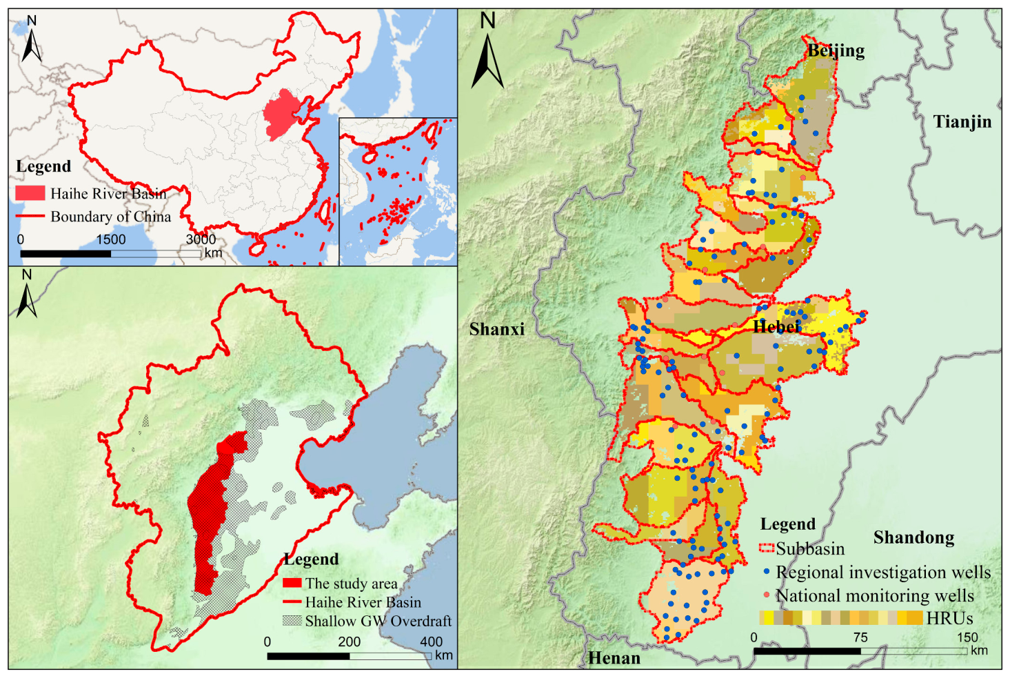
This study focuses on the piedmont alluvial plain of the Taihang Mountains in Hebei Province, situated within the Haihe River basin of northern China (Figure 1). The basin encompasses China’s political and economic heartland—including Beijing and Tianjin—yet supports approximately 10% of the national population with per capita water resources less than one-tenth of the global average, making it one of the most acutely water-stressed yet agriculturally productive regions on Earth [7,35]. The study area spans 36°07′ N–39°35′ N and 114°17′ E–116°14′ E, encompassing approximately 22,753 km² across 48 counties in the jurisdictions of Baoding, Shijiazhuang, Xingtai, and Handan. Cropland covers roughly 80% of the area (~18,200 km²), dominated by the winter wheat (Triticum aestivum L.)–summer maize (Zea mays L.) double-cropping system [11].

Groundwater-fed irrigation in this region has a half-century history of escalating exploitation. Large-scale well drilling expanded rapidly from the 1970s onward as surface water availability collapsed following the construction of numbers of upstream reservoirs and a precipitation decline that left most rivers seasonally dry by the 1990s [7,36]. Extraction peaked around 2012, by which time cumulative overdraft across the Haihe Plain had reached approximately 180 billion m³ [37]. Since 2014, the Chinese government has deployed a broad portfolio of countermeasures—including the South-to-North Water Diversion Project, fallow programs, and closure of partly pumping wells—which have triggered measurable water-table recovery in urban areas [38,39,40] Nevertheless, in the agricultural hinterland—including the study area—irrigation pumping continues to drive a persistent negative groundwater balance, underscoring the urgency of the scientific challenge this study addresses [17,41].

2.2. The SWAT-GW Model

The training dataset for the gray-box ML framework was generated using a groundwater-module-enhanced version of the Soil and Water Assessment Tool (SWAT-GW) that has been developed, calibrated, and progressively refined for this study area [11]. This model retains the continuous-time, semi-distributed structure of SWAT, in which the soil–plant–atmosphere–groundwater system is simulated at a daily time step for hydrological response units (HRUs). The standard SWAT groundwater module represents the shallow and deep aquifers as water-balance reservoirs but does not directly calculate groundwater-table depth in an intensively pumped plain. The model was therefore enhanced by introducing the shallow-aquifer bottom depth (SHBD), aquifer porosity (SHPOR), specific yield (GWSPYLD), and lateral recharge from the adjacent Taihang Mountains (LARCHRG) [11]. At daily time step $i$, the shallow-aquifer storage balance is expressed as

$$SHALLIS{T}_i=SHALLIS{T}_{i-1}+W_{rchrg}-Q_{gw}-W_{revap}-W_{deep}-W_{pump,sh}+W_{larchrg}$$

(1)

where $SHALLIS{T}_i$ is the amount of water stored in the shallow aquifer on day $i$ (mm), $SHALLIS{T}_{i-1}$ is the amount of water stored in the shallow aquifer on day $i-1$ (mm), $W_{rchrg}$ is the amount of vertical recharge entering the aquifer on day $i$ (mm), $Q_{gw}$ is the groundwater flow, or base flow, into the main channel on day $i$ (mm), $W_{revap}$ is the amount of water moving into the soil zone in response to water deficiencies on day i (mm), $W_{deep}$ is the amount of water percolating from the shallow aquifer into the deep aquifer on day $i$ (mm), ${\mathrm{W}}_{pump,sh}$ is the amount of water removed from the shallow aquifer by pumping on day $i$ (mm), and $W_{larchrg}$ is the amount of lateral recharge from mountainous area entering the aquifer on day $i$ (mm). Storage change is converted to groundwater-table depth using

$$SHGW{T}_i=SHGW{T}_{i-1}-{\displaystyle \frac{SHALLIS{T}_i-SHALLIS{T}_{i-1}}{GWSPYLD\times 1000}}$$

(2)

where $SHGW{T}_i$ is the shallow groundwater table depth on day $i$ (m); $SHGW{T}_{i-1}$ is the shallow groundwater table depth on day $i-1$ (m); and GWSPYLD is the specific yield of the shallow aquifer. Groundwater-table depth is calculated at the HRU scale and aggregated to the subbasin scale using an area-weighted mean. The full initialization, threshold, storage-balance, water-table conversion, and spatial-aggregation equations are provided in Supplementary Materials [42].

The model was simulated for 1990–2012, with 1990–1992 used as a three-year warm-up period. Initial shallow-aquifer storage was calculated from the initial groundwater-table depth, SHBD, and SHPOR. Hydrogeological parameters were first initialized using regional investigation and groundwater-resource-assessment data to maintain physically realistic ranges. Following sensitivity analysis, GWSPYLD, GW_DELAY, RCHRG_DP, and soil saturated hydraulic conductivity (SOL_K) were further calibrated using the SUFI-2 algorithm in SWAT-CUP. Uncertainty was represented by the 95% prediction uncertainty generated through Latin hypercube sampling. Two complementary shallow-groundwater observation datasets supplied by the China Institute of Geo-environmental Monitoring were used (Figure 1). Continuous monthly records from 16 national monitoring wells during 1993–2010 were used for dynamic calibration; for each subbasin with national monitoring coverage, the well closest to the subbasin’s center was selected. Annual observations from 148 regional investigation wells during 2006–2012 were used for spatial validation, with measurements from wells in the same subbasin averaged at each survey time. Five subbasins in the northern plain of the Ziya River basin (ZYHP) lacked national monitoring wells; in these subbasins, half of the regional investigation wells were used for calibration and the remaining half for validation.

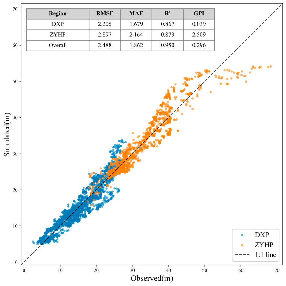
The calibrated model achieved R² > 0.95 and NSE > 0.95 for shallow groundwater table dynamics across all 22 subbasins, with additional validation against remote-sensing-derived actual evapotranspiration, statistical crop yield records, and GRACE satellite-based groundwater storage change estimates [11,43]. Furthermore, to provide a comprehensive evaluation of the calibration accuracy, the Global Performance Indicator (GPI) [44] was calculated. The resulting highly accurate GPI evaluation (Figure 2) further corroborates the robustness of the simulated groundwater dynamics. Because the principal advantage of the enhanced SWAT framework is its simultaneous representation of the soil–plant–atmosphere continuum and groundwater system, model evaluation was not restricted to groundwater-table depth. Independent multi-objective checks included remote-sensing determinations of actual evapotranspiration, statistical winter-wheat and summer-maize yields, tracer-based groundwater recharge, and groundwater-balance components from regional groundwater-resource assessments. Following groundwater-module calibration, simulated annual actual evapotranspiration was 633.0 ± 40.0 mm, compared with 609.0 ± 47.8 mm from remote sensing, with a mean subbasin R² value of 0.77. Simulated winter-wheat and summer-maize yields had subbasin NRMSE ranges of 8–21% and 12–22%, respectively. At the Luquan and Luancheng sites, tracer-based annual recharge was 177–239 mm [45], compared with 173–202 mm simulated by the model. At the regional scale, simulated recharge and shallow-aquifer storage depletion were 237 and 159 mm yr⁻¹, respectively, within the independently assessed ranges of 235–246 and 131–179 mm yr⁻¹ [11,46]. These multiple lines of evidence support the consistency of the coupled SPAC–groundwater simulation. Building on this validated platform, subsequent studies have systematically applied the model to evaluate limited irrigation schemes [15], seasonal fallow strategies [16], sprinkler irrigation feasibility [41], multi-cropping–irrigation coupling [17], and regional irrigation water allocation optimization [47]. The present study draws directly on this established modeling infrastructure; full details of the model establishment, parameterization, and calibration are provided in Zhang et al. [11].

2.3. Gradient Irrigation Scenario Design and Response Variable Extraction

To construct the paired datasets required for fitting irrigation–groundwater response functions, a series of gradient irrigation scenarios was designed within the validated SWAT-GW framework. Because shallow groundwater depletion in the study area is driven predominantly by pumping during the winter-wheat growing season, the scenarios were applied exclusively to winter-wheat irrigation (IRRWW), with summer-maize irrigation, climate forcing, and soil parameters held constant.

A non-uniform sampling strategy was adopted to balance resolution against efficiency across the full irrigation continuum (0–400+ mm). Gradient points were densely spaced in the 0–100 mm range to capture the recharge–abstraction equilibrium threshold and the nonlinear infiltration behavior of the unsaturated zone under water-limited conditions, and more sparsely above 300 mm, where scenario-specific amounts correspond to farmer-adjusted pumping under dry, normal, and wet precipitation years. For each hydrological response unit (HRU), 15 irrigation levels were constructed. Taking HRU 00040001 as a representative example, the levels span 0, 30, 40, 50, 60, 70, 75, 80, 90, 150, 225, 300, 368, 405, and 438 mm—from completely rain-fed conditions to full conventional irrigation.

All scenarios were simulated over a 20-year period, yielding 21,000 data records (70 HRUs × 15 levels × 20 years). For each HRU–irrigation combination, three groundwater response variables were extracted: (1) GW_RCHG (mm), the vertical recharge flux from the soil profile to the shallow aquifer; (2) SA_ST (mm), the net change in shallow aquifer storage, integrating all recharge and discharge components; and (3) SHGWT (m), the mean shallow groundwater table depth, reflecting the integrated aquifer response to recharge, lateral flow, deep percolation, and pumping. The paired datasets of IRRWW versus each response variable constitute the empirical basis for the methods described in Section 3 (Methods).

3. Methods

3.1. Machine Learning Target Variables and Feature Variables

The defining feature of the gray-box framework is that the ML prediction targets are not groundwater state variables themselves, but the coefficients of polynomial functions that govern how these variables respond to irrigation. For each HRU, three candidate polynomial forms—linear (y = ax + b), quadratic (y = ax² + bx + c), and cubic (y = ax³ + bx² + cx + d)—were fitted via Ordinary Least Squares to the relationship between winter-wheat irrigation intensity (IRR, mm) and each of three annual groundwater response variables. The three response variables are as follows: annual recharge to the shallow aquifer (Recharge, equivalent to GW_RCHG in the SWAT-GW output, mm yr⁻¹), annual net change in shallow aquifer storage (Storage, equivalent to SA_ST, mm yr⁻¹), and annual change in shallow groundwater table depth (Water Table, equivalent to SHGWT, m yr⁻¹). Physically, Recharge increases monotonically with irrigation as more water percolates past the root zone; Storage and Water Table, by contrast, both decline as pumping increasingly outpaces the recharge gains, reflecting a persistent net loss from the aquifer. The contrasting monotonic directions of these three responses provide a natural internal consistency check on the fitted functions. The optimal polynomial order was determined by comparing goodness-of-fit and residual patterns across all HRUs (results in Section 4.1), and the coefficients of the selected order define the multi-output target vector for ML training.

The 26 input features (

Table 1. Environmental and hydrogeological input features for the ML models.

No.	Variable	Unit	Physical Description
Soil properties (upper layer: 0–30 cm; lower layer: 30–200 cm)
1	Clay_Up	%	Clay content, upper layer
2	Clay_Down	%	Clay content, lower layer
3	Sand_Up	%	Sand content, upper layer
4	Sand_Down	%	Sand content, lower layer
5	Silt_Up	%	Silt content, upper layer
6	Silt_Down	%	Silt content, lower layer
7	OC_Up	%	Organic carbon content, upper layer
8	OC_Down	%	Organic carbon content, lower layer
9	AWC_Up	mm/mm	Available water capacity, upper layer
10	AWC_Down	mm/mm	Available water capacity, lower layer
11	BD_Up	Mg/m3	Bulk density, upper layer
12	BD_Down	Mg/m3	Bulk density, lower layer
13	K_Up	mm/hr	Saturated hydraulic conductivity, upper layer
14	K_Down	mm/hr	Saturated hydraulic conductivity, lower layer
Meteorological variables
15	SOLAR	MJ/m2	Annual mean daily solar radiation
16	TMP_AV	°C	Annual mean temperature
17	TMP_MN	°C	Annual mean minimum temperature
18	TMP_MX	°C	Annual mean maximum temperature
19	PCP_RY	mm	Annual precipitation
20	PCP_SM	mm	Precipitation during summer-maize season
21	PCP_WW	mm	Precipitation during winter-wheat season
Hydrogeological parameters
22	RCHRG_DP	–	Deep aquifer percolation fraction
23	LARCHRG	mm	Lateral recharge from Taihang Mountains
24	GW_SPYLD	m3/m3	Specific yield of the shallow aquifer
25	GW_DELAY	days	Groundwater delay time through vadose zone
Management variable
26	IRR_SM	mm	Summer-maize irrigation amount

; Figure S6) were selected to represent the physical chain through which irrigation water travels from the surface to the aquifer. Soil properties (e.g., bulk density, available water capacity, and saturated hydraulic conductivity) govern infiltration and vadose-zone redistribution. Meteorological variables (e.g., temperature, radiation, and precipitation) control evapotranspiration demand and antecedent soil moisture. Hydrogeological parameters (e.g., specific yield, groundwater delay time, and lateral recharge) determine the aquifer’s storage capacity and response timescale. Summer-maize irrigation is included as the sole management variable, because it sets the soil moisture baseline inherited by the subsequent winter-wheat season. The dataset was split 70/30 into training and testing subsets, and all target coefficients were standardized to zero mean and unit variance prior to training.

3.2. Inversion of Hydrogeological Parameters from Response Functions

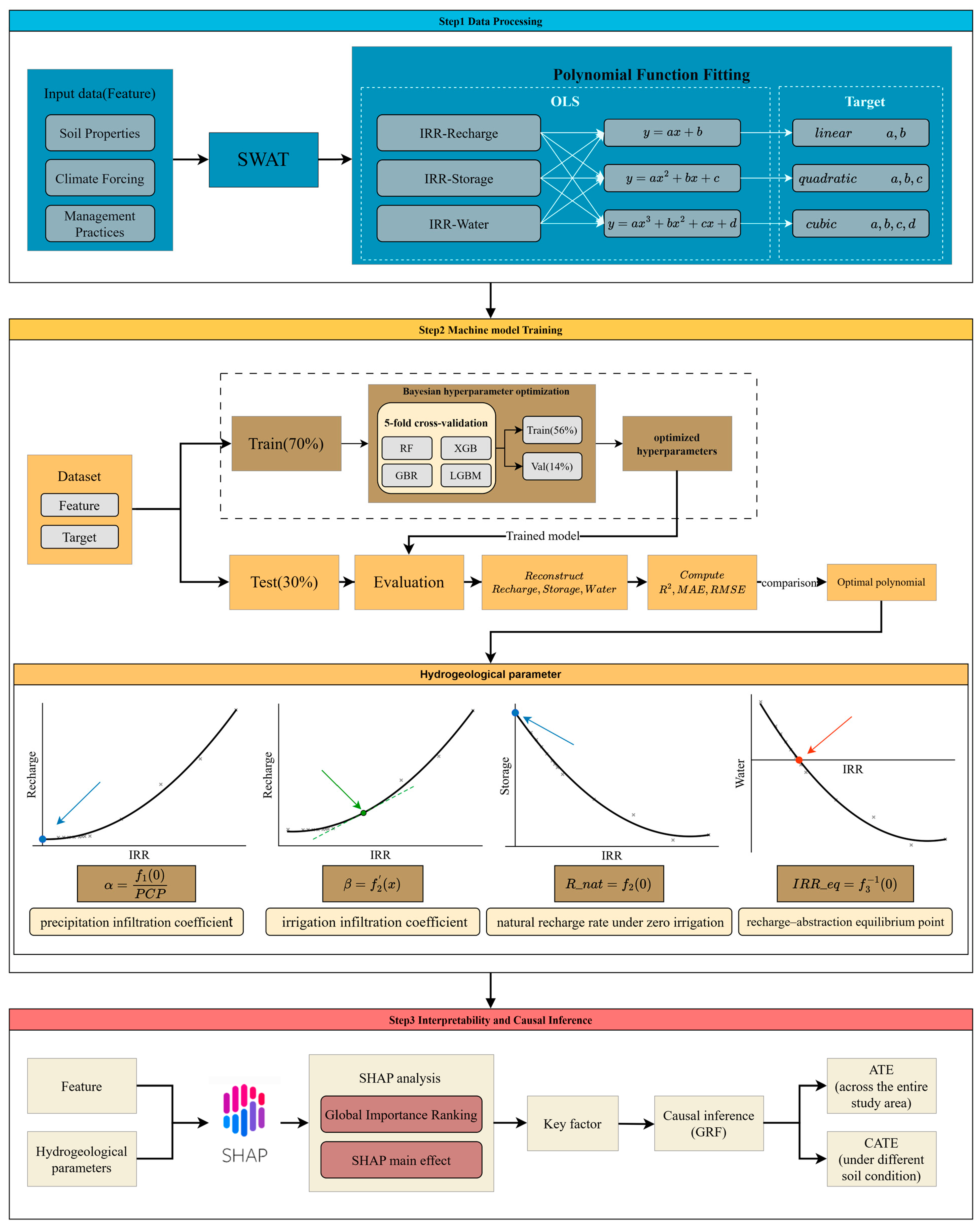
Beyond predicting the full irrigation–groundwater response curve, the gray-box framework enables the extraction of four management-critical hydrogeological parameters directly from the geometric properties of the fitted functions (Figure 3).

For the IRR–Recharge function y = f₁(x), x is winter-wheat irrigation (mm) and y is annual vertical recharge ($\mathrm{mm}\cdot {\mathrm{yr}}^{-1}$); the y-intercept f₁(0) represents the recharge generated under zero irrigation. The ratio α = f₁(0)/PCP yields the precipitation infiltration coefficient, a standard parameter in groundwater resource assessment [29,30]. The first derivative f₁′(x) quantifies the marginal recharge gain per unit irrigation increment, and is interpreted as the irrigation infiltration coefficient β [31].

For the IRR–Storage function y = f₂(x), y is annual net change in shallow aquifer storage ($\mathrm{mm}\cdot {\mathrm{yr}}^{-1}$) and the y-intercept R_nat = f₂(0) represents the storage balance under zero irrigation, integrating vertical precipitation-derived percolation and lateral recharge from the Taihang Mountains, minus natural discharge. This quantity—the natural recharge—reflects the total renewable resource baseline of the aquifer, and differs from α in that it encompasses all recharge pathways rather than isolating the vertical precipitation component alone [32,48].

For the IRR–Water Table function y = f₃(x), where y is annual change in shallow groundwater table depth ($\mathrm{m}\cdot {\mathrm{yr}}^{-1}$, negative indicating decline), the root IRR_eq satisfying f₃(IRR_eq) = 0 identifies the recharge–abstraction equilibrium point—the threshold irrigation intensity at which water-table decline ceases. Unlike R_nat, this quantity incorporates irrigation return flow: IRR_eq marks the intensity at which total recharge (natural plus irrigation-derived) exactly offsets total discharge [33,34].

These four parameters—α, β, R_nat, and IRR_eq—are fully determined by the polynomial coefficients predicted by the ML models, enabling rapid parameter inference for any new combination of environmental inputs without re-running the numerical model.

3.3. Ensemble Machine Learning Algorithms

The theoretical basis of the machine learning algorithms employed in this study lies in ensemble learning, a paradigm that combines multiple weak learners to construct a highly accurate and robust predictive model. Depending on how the base learners (decision trees) are generated and aggregated, the four selected algorithms—Random Forest [49], Gradient Boosting Regression (GBR) [50], XGBoost [51], and LightGBM [52]—are driven by two distinct theoretical principles: Bagging and Boosting.

Bagging (Bootstrap Aggregating): Random Forest (RF) operates on the theoretical principle of variance reduction. It constructs an ensemble of independent decision trees trained on bootstrap samples of the dataset. To ensure decorrelation among the trees, RF selects a random subset of environmental features at each node split. The final prediction is the average of all individual tree outputs, which effectively mitigates model overfitting.

Boosting: The remaining three algorithms belong to the boosting family, which is founded on the theoretical principle of bias reduction. They train weak learners sequentially, and each subsequent tree focuses on minimizing the residual errors (or loss gradients) of the previous ensemble. The overall prediction takes the following general additive form:

$$F\left(x\right)=f_0\left(x\right)+{\displaystyle \sum _{m=1}^M}\eta f_m\left(x\right)$$

(3)

where $f_0\left(x\right)$ is the initial base prediction, $f_m\left(x\right)$ is the $m$-th decision tree, $\eta \in (0,1]$ is the learning rate, and $M$ is the total number of iterations.

Within this shared boosting framework, each algorithm introduces specific theoretical optimizations. Specifically, GBR fits each new tree to the negative first-order gradient of a differentiable loss function. Building upon this gradient-based approach, XGBoost optimizes the objective function by employing a second-order Taylor expansion (utilizing both gradients and Hessians) and introduces explicit $L_1$ and $L_2$ regularization terms to structurally penalize tree complexity. Furthermore, LightGBM improves scalability and computational efficiency via Gradient-based One-Side Sampling (GOSS), which retains instances with large gradients while randomly dropping those with small gradients, alongside Exclusive Feature Bundling (EFB) to reduce feature dimensionality.

Since all four algorithms are natively single-output, each was wrapped within a MultiOutputRegressor framework (scikit-learn, version 1.6.1) that trains independent base regressors for each target coefficient in parallel.

Hyperparameters for each algorithm were tuned via Bayesian optimization using BayesSearchCV from the scikit-optimize library (version 0.10.2) [53], which constructs a Gaussian process surrogate of the cross-validation score surface and uses an acquisition function to balance exploration and exploitation. The procedure was run for 100 iterations with 5-fold cross-validation. The hyperparameter search spaces are summarized in

Table 2. Hyperparameter search spaces for the four ensemble learning algorithms.

Algorithm	Hyperparameter	Type	Search Space
RF	n_estimators	Int	[300, 1200]
	max_depth	Int	[10, 100]
	min_samples_split	Int	[2, 20]
	min_samples_leaf	Int	[1, 10]
	max_features	Real	[0.1, 0.9]
GBR	n_estimators	Int	[300, 1200]
	max_depth	Int	[3, 5]
	min_samples_split	Int	[2, 5]
	min_samples_leaf	Int	[1, 5]
	learning_rate	Real	[0.05, 0.1]
XGBoost	n_estimators	Int	[800, 2000]
	max_depth	Int	[4, 8]
	learning_rate	Real	[0.01, 0.15]
	subsample	Real	[0.6, 1.0]
	reg_alpha	Real	[0, 20]
	reg_lambda	Real	[0, 20]
LightGBM	n_estimators	Int	[300, 1200]
	max_depth	Int	[2, 5]
	learning_rate	Real	[0.05, 0.2]
	reg_alpha	Real	[0, 0.01]
	reg_lambda	Real	[0, 0.01]

. Model performance was evaluated on the held-out test set (30%) using the coefficient of determination (R²) and root mean square error (RMSE) for each predicted coefficient.

3.4. Progressive Feature Ablation Under Data Scarcity

Most groundwater over-exploitation zones globally lack the granular hydrogeological and irrigation monitoring data available in intensively instrumented regions such as the North China Plain. To evaluate the operational potential of the gray-box framework under realistic data constraints, the 26 input features were stratified into three hierarchical tiers based on their real-world accessibility (

Table 3. Feature accessibility tiers for the progressive ablation experiment.

Data Tier	Accessibility	Category	Variables
Tier 1	Easy	Meteorological forcing	PCP_SM, PCP_RY, PCP_WW, TMP_AV, TMP_MX, TMP_MN, SOLAR
		Basic soil properties	Clay_Up, Clay_Down, Silt_Up, Silt_Down, Sand_Up, Sand_Down, OC_Up, OC_Down, BD_Up, BD_Down
Tier 2	Moderate	Soil hydraulic parameters	K_Up, K_Down, AWC_Up, AWC_Down
		Agricultural management	IRR_SM
Tier 3	Difficult	Hydrogeological parameters	GW_DELAY, RCHRG_DP, LARCHRG, GW_SPYLD

Note: The three ablation scenarios are constructed by progressively expanding the feature set: Tier 1 only → Tier 1 + 2 → Tier 1 + 2 + 3 (full feature set).

). Tier 1 (easily accessible) comprises meteorological forcing variables and basic soil physical properties (texture, organic carbon, and bulk density) that are routinely available from national meteorological networks and standard soil surveys. Tier 2 (moderately accessible) supplements Tier 1 with soil hydraulic parameters (saturated hydraulic conductivity and available water capacity) and agricultural management records (summer-maize irrigation), which require dedicated field measurement or regional datasets. Tier 3 (the full feature set) additionally incorporates deep-seated hydrogeological parameters—groundwater delay time (GW_DELAY), deep percolation fraction (RCHRG_DP), lateral recharge (LARCHRG), and specific yield (GW_SPYLD)—that are the most difficult and costly to acquire, typically requiring multi-year groundwater investigations or model calibration.

Three ablation scenarios were constructed by progressively expanding the feature set from Tier 1 alone, to Tiers 1 + 2, and finally to the complete Tier 1 + 2 + 3 set. At each scenario, all four ML algorithms were retrained and re-evaluated on the same held-out test set, with R² and RMSE compared against the full-feature baseline. This cumulative design simulates the real-world gradient from data-scarce to data-rich conditions and identifies the minimum feature set required for operationally useful coefficient prediction.

3.5. SHAP Analysis and Causal Forest

To interpret the trained ML models, two complementary analytical frameworks were applied: SHAP for feature attribution and Causal Forest for causal effect estimation.

The SHAP (SHapley Additive exPlanations) framework [54] decomposes each prediction into additive contributions from individual features based on Shapley values from cooperative game theory. For a model f and an input vector x, the prediction is expressed as

$$f\left(\mathrm{x}\right)={\varphi }_0+{\displaystyle \sum _{j=1}^p}{\varphi }_j$$

(4)

where ${\varphi }_0$ is the baseline (expected) prediction, and $p$ is the total number of features. Positive ${\varphi }_j$ indicates that feature $j$ increases the prediction relative to the baseline, while negative values indicate a decreasing effect.

Formally, the SHAP value for feature $j$ is defined as

$${\varphi }_j=\sum _{S\subseteq \mathcal{F}\setminus \left\{j\right\}}{\displaystyle \frac{\mid S\mid !(p-\mid S\mid -1)!}{p!}}\left[f(S\cup \{j\left\}\right)-f\left(S\right)\right]$$

(5)

where: $\mathcal{F}$ is the set of all features, $S$ is a subset of features excluding $j$, $f\left(S\right)$ denotes the model prediction using only the features in $S$, and $\mid S\mid$ is the cardinality of $S$. In this study, both global SHAP importance (mean absolute Shapley values across all samples) and local SHAP dependence plots were used to identify the dominant drivers of each polynomial coefficient.

While SHAP quantifies feature importance, it captures associational rather than causal relationships. To advance from correlation to causation, we employed Causal Forest, a non-parametric causal inference method based on Generalized Random Forests [55,56]. Causal Forest estimates the Conditional Average Treatment Effect (CATE):

$$\tau \left(x\right)=E\left[Y\left(1\right)-Y\left(0\right)|X=x\right]$$

(6)

where $Y\left(1\right)$ and $Y\left(0\right)$ denote the potential outcomes under treatment and control conditions, respectively, and $x$ is the covariate vector. In this study, the treatment variable is annual precipitation (PCP_RY)—treated as a continuous variable—and the outcome variables are IRR_eq and β. The Causal Forest estimates the conditional average treatment effect (CATE) $\tau \left(x\right)=E\left[Y\left(1\right)-Y\left(0\right)|X=x\right]$, where $Y\left(1\right)$ and $Y\left(0\right)$ denote the potential outcomes under a one-unit increase in precipitation versus the control level. The average treatment effect (ATE) is then obtained as $E\left[\tau \left(X\right)\right]$. The Average Treatment Effect (ATE = E[τ(x)]) quantifies the overall causal impact of precipitation regime on aquifer sustainability, while the spatially resolved CATE reveals how this causal effect varies across hydrogeological settings. The Causal Forest was implemented using the grf package in R (version 4.5.2) [57]. The complete methodological workflow of this study is illustrated in Figure 3.

3.6. Statistical Evaluation Metrics

To rigorously evaluate both the goodness-of-fit for the polynomial response functions and the predictive performance of the machine learning algorithms, a comprehensive set of statistical metrics was employed. Standard metrics, including the ordinary coefficient of determination ($R^2$), root mean square error (RMSE), and mean absolute error (MAE), were utilized to measure the overall variance explanation and absolute deviations. Their mathematical expressions are as follows:

$$R^2=1-{\displaystyle \frac{{\displaystyle {\sum }_{i=1}^n}{\left(y_i-{\hat{y}}_i\right)}^2}{{\displaystyle {\sum }_{i=1}^n}{\left(y_i-\overline{y}\right)}^2}}$$

(7)

$$RMSE=\sqrt{{\displaystyle \frac{1}{n}}{\displaystyle \sum _{i=1}^n}{\left(y_i-{\hat{y}}_i\right)}^2}$$

(8)

$$MAE={\displaystyle \frac{1}{n}}{\displaystyle \sum _{i=1}^n}\left|y_i-{\hat{y}}_i\right|$$

(9)

where $n$ is the total number of samples, $y_i$ represents the target value (e.g., SWAT-GW simulated data), ${\hat{y}}_i$ represents the model-fitted or ML-predicted value, and $\overline{y}$ is the mean of the target values.

Furthermore, to prevent over-parameterization when comparing polynomial functions of varying degrees, the adjusted coefficient of determination ($R_{adj}^2$) was adopted. $R_{adj}^2$ penalizes the addition of unnecessary terms, ensuring that model complexity is mechanistically justified [58]. It is calculated as

$$R_{adj}^2=1-{\displaystyle \frac{\left(1-R^2\right)\left(n-1\right)}{n-p}}$$

(10)

where $n$ is the number of samples and $p$ is the number of fitting parameters.

Additionally, considering that large-scale hydrogeological datasets often exhibit non-normal distributions (such as skewed groundwater table fluctuations), traditional metrics like RMSE might be overly sensitive to extreme outliers. To address this, the Hanna and Heinold (HH) index was introduced as a robust alternative error metric [44]. The HH index is particularly effective in penalizing proportional errors regardless of data normality, and is expressed as

$$HH={\displaystyle \frac{{\displaystyle {\sum }_{i=1}^n}{\left(y_i-{\hat{y}}_i\right)}^2}{{\displaystyle {\sum }_{i=1}^n}\left(y_i\cdot {\hat{y}}_i\right)}}$$

(11)

where ${\mathit{y}}_{\mathit{i}}$ and ${\stackrel{\mathit{ˆ}}{\mathit{y}}}_{\mathit{i}}$ represent the SWAT-GW simulated and polynomial-fitted (or ML-predicted) values, respectively. A lower HH index indicates superior model accuracy.

4. Results

4.1. Selection of the Optimal Polynomial Order: Fitting Accuracy and ML Learnability

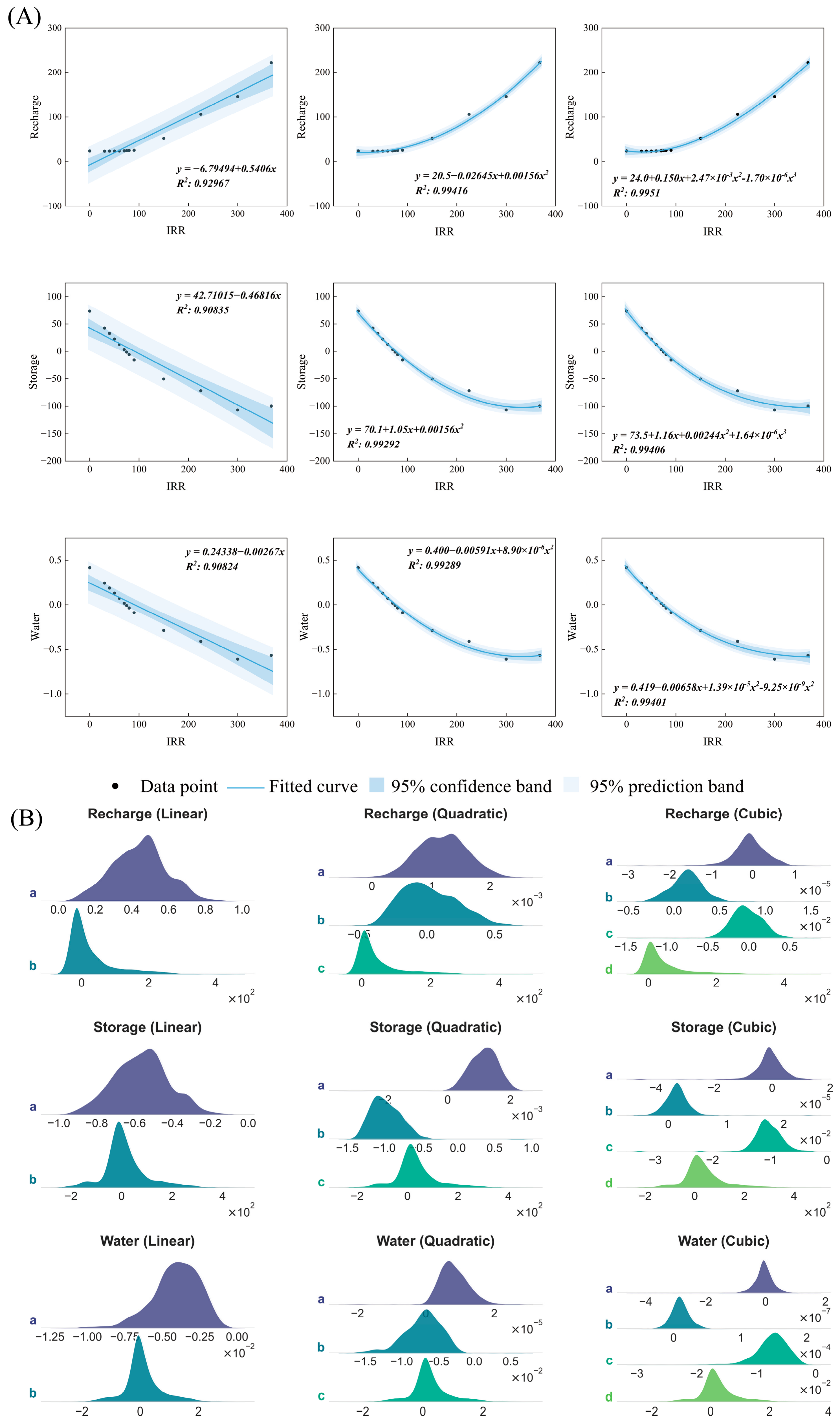
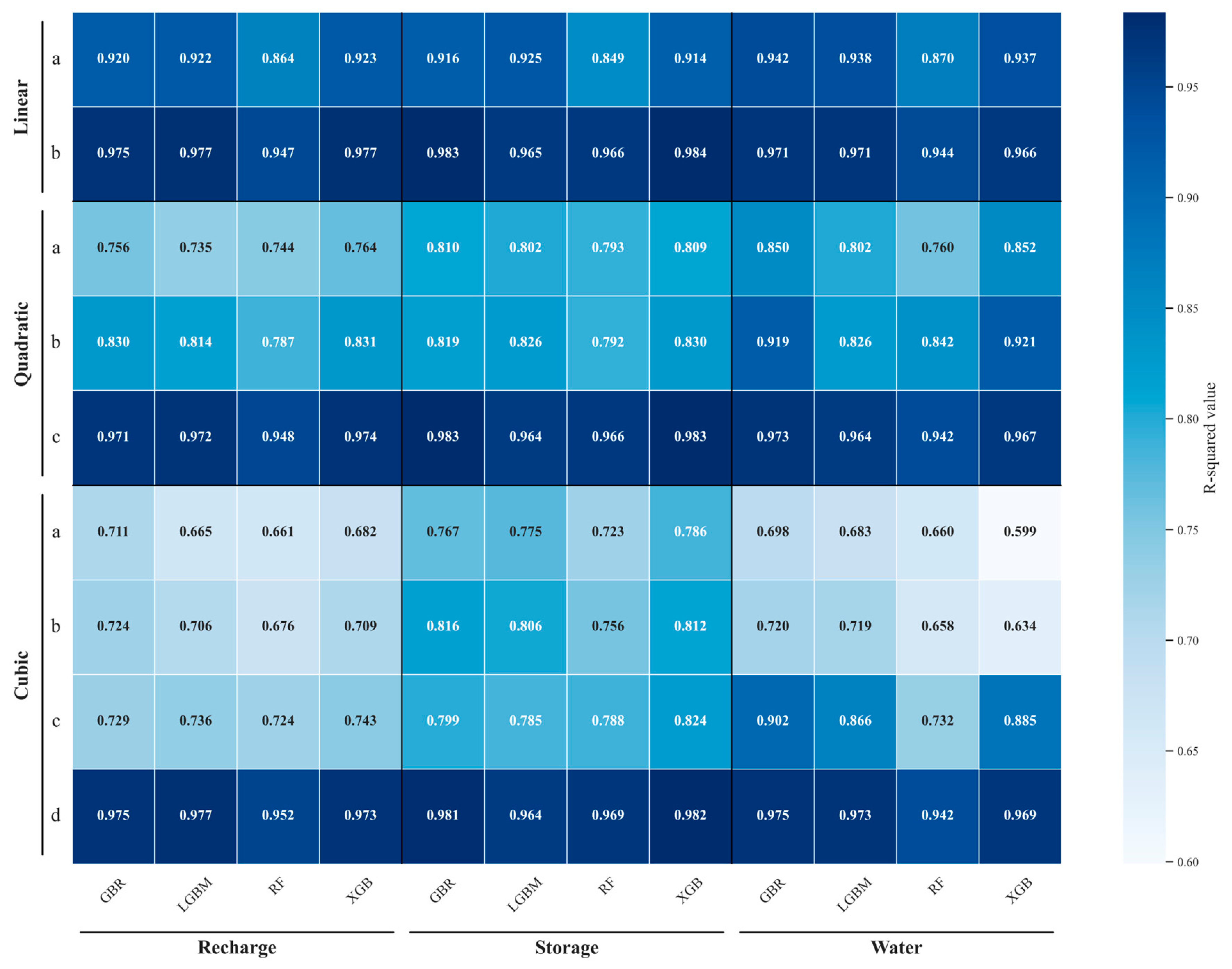
Linear, quadratic, and cubic polynomials were fitted to the IRR–Recharge, IRR–Storage, and IRR–Water Table relationships for all 70 HRUs (Figure 4A;

Table 4. Fitting accuracy of linear, quadratic, and cubic polynomial forms across three groundwater response variables (averaged over all 70 HRUs).

Variable	Function	RMSE	MAE	R2	HH	R2_adj
Recharge	Linear	13.05	9.85	0.979	0.210	0.897
	Quadratic	5.68	3.83	0.996	0.081	0.978
	Cubic	4.28	2.79	0.998	0.056	0.988
Storage	Linear	14.25	10.06	0.983	0.145	0.933
	Quadratic	8.29	4.34	0.994	0.065	0.979
	Cubic	6.15	3.23	0.996	0.050	0.986
Water Table	Linear	0.11	0.07	0.983	0.145	0.933
	Quadratic	0.06	0.03	0.994	0.065	0.979
	Cubic	0.05	0.02	0.997	0.050	0.986

), and the corresponding coefficient sets were independently predicted by four ensemble ML algorithms (Figure 5).

From a fitting perspective, the linear form yields R² values of 0.908–0.983 but cannot reproduce two physically essential features: the diminishing marginal groundwater storage and water table response at high irrigation intensities (300–400 mm), and the accurate zero-irrigation intercept that underpins parameter inversion (Figure 4A). The quadratic form resolves both deficiencies, raising R² above 0.994 and R²_adj above 0.978 for all three variables. The cubic form provides only marginal further improvement (e.g., R² from 0.996 to 0.998 for Recharge), with its leading coefficient a on the order of 10⁻⁵ to 10⁻⁷—contributing negligibly to the functional shape (Figure 4B).

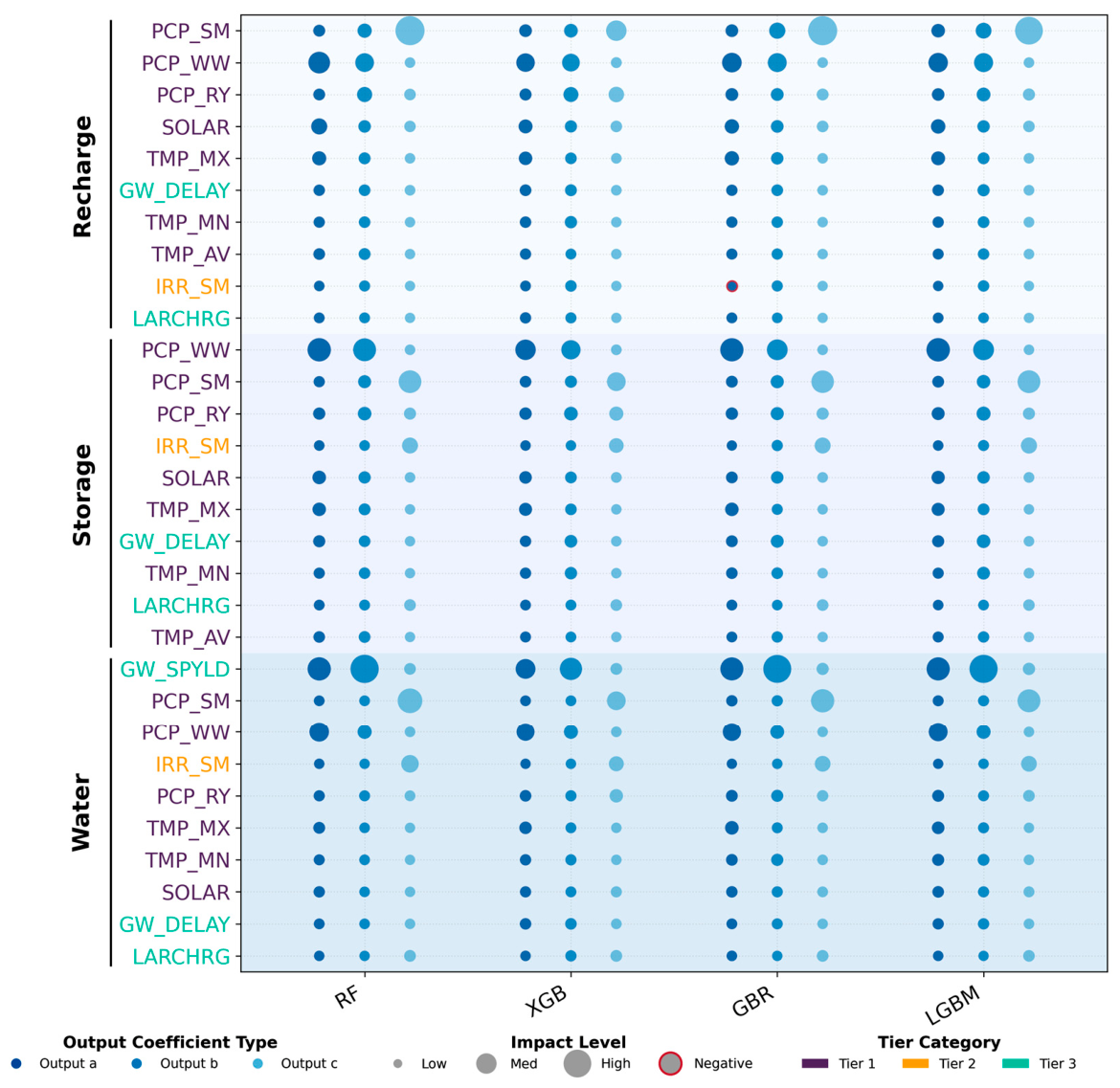
From an ML learnability perspective, however, the three polynomial orders diverge sharply (Figure 5). The linear coefficients (a, b) are well-predicted across all four algorithms (R² generally > 0.90), but this advantage is moot, given the linear form’s physical inadequacy in failing to capture the inherent nonlinear hydrogeological behaviors, such as the diminishing marginal gains of aquifer recharge. The quadratic coefficients exhibit a clear identifiability hierarchy: the intercept term c—physically representing the zero-irrigation baseline—is the most learnable (R² = 0.94–0.98), followed by the linear term b (R² = 0.79–0.92) and the quadratic term a (R² = 0.74–0.85). The cubic coefficients, by contrast, show a pronounced degradation in the high-order terms: the cubic coefficient a and quadratic coefficient b are predicted with R² values as low as 0.60–0.79, and for SHGWT the cubic a-coefficient drops to 0.599—indicating that the ML models cannot reliably resolve coefficients the magnitudes of which span several orders below those of the lower-order terms. More importantly, from an ML perspective, predicting four interdependent cubic coefficients introduces severe noise and sensitivity, leading to a significant degradation in prediction reliability. In conclusion, the quadratic coefficients remained tractable and learnable, whereas cubic coefficients showed significant degradation in prediction reliability.

This joint assessment—fitting accuracy from below, ML learnability from above—converges on the quadratic form as the optimal choice. It offers sufficient nonlinearity to capture the physically meaningful curvature, high fitting accuracy (R² > 0.994), a coefficient set that remains tractable for ML prediction, and interpretable hydrogeological content (Section 3.3). All subsequent results are based on the quadratic polynomial. The physical rationale for why the quadratic form constitutes a reasonable approximation of the governing processes is discussed in Section 5.1.

4.2. Prediction Robustness Under Data Scarcity

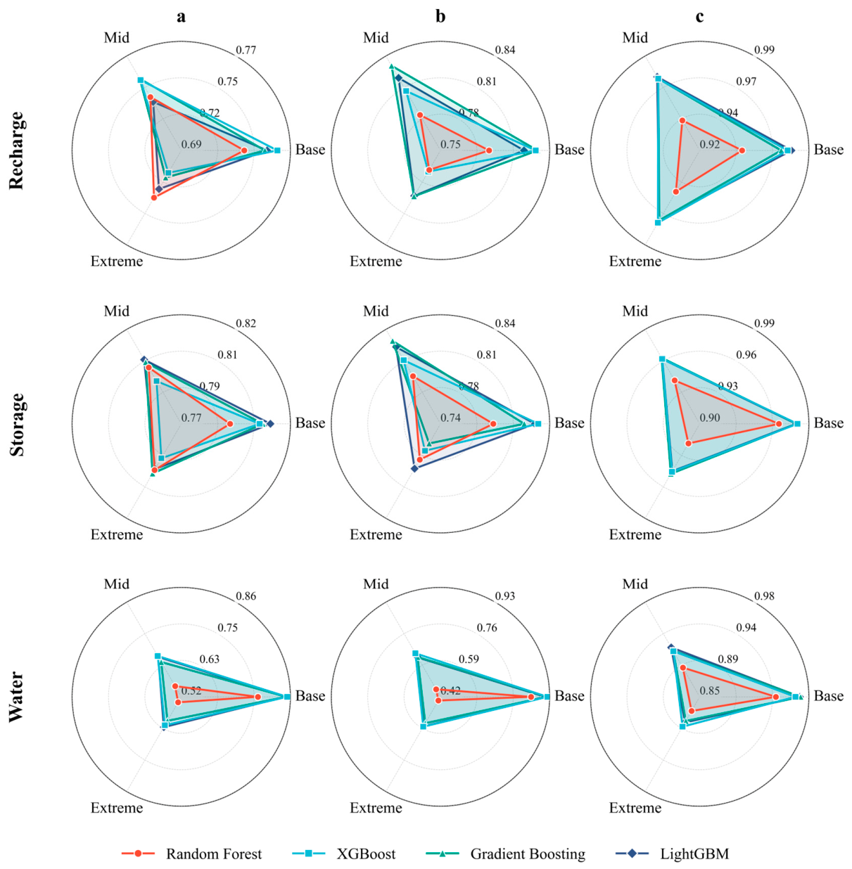
The gray-box framework was tested under three progressively expanding feature scenarios—Tier 1 only (meteorological forcing and basic soil properties), Tier 1 + 2 (adding soil hydraulic parameters and summer-maize irrigation), and the full feature set (adding hydrogeological parameters)—to evaluate how prediction accuracy degrades as data availability diminishes (Figure 6).

The degradation follows a physically interpretable gradient across the three response variables. The IRR–Recharge coefficients prove the most resilient: under the Extreme (Tier 1 only) scenario, R² for coefficients a, b, and c declines by only 3.44%, 3.17%, and 0.18% relative to the full-feature baseline, respectively (averaged across four algorithms). The IRR–Storage coefficients show moderate sensitivity, with c retaining R² > 90% under Tier 1 but a and b declining by 1.08% and 4.19%. The IRR–Water Table coefficients are the most vulnerable—a and b lose 23.10% and 35.93% of their baseline R² under Tier 1, while c degrades more gently (from 96.36% to 88.27%, an 8.09% reduction). This ordering—Recharge the most robust, Storage intermediate, Water Table most sensitive—mirrors a fundamental physical hierarchy: predicting how much water reaches the aquifer (a flux quantity) relies primarily on atmospheric and soil information, whereas predicting how the water table responds (a state quantity) additionally requires knowledge of aquifer storage properties, most critically the specific yield. This stark contrast provides a critical guideline for practical applications: in unmonitored or data-scarce regions, the gray-box framework can still provide reliable estimates of recharge dynamics, but accurately predicting water-table responses strictly necessitates high-fidelity hydrogeological data.

Among the four algorithms, boosting methods (XGBoost, GBR, and LightGBM) consistently outperform RF for the most challenging prediction targets—the Water Table coefficients and the intercept c across all three variables—regardless of data availability tier. For the relatively easier targets (e.g., Recharge a and b under extreme scarcity), however, the performance gap narrows and RF occasionally matches or slightly exceeds individual boosting algorithms, likely because its bagging-based averaging mechanism provides greater stability when the feature space is severely constrained.

The Permutation Importance analysis (Figure 7) reveals the physical drivers behind these patterns. For Recharge and Storage, precipitation dominates during both cropping seasons (PCP_WW, PCP_SM), followed by temperature and solar radiation—which control evapotranspiration and thereby regulate the fraction of water available for deep percolation. Summer-maize irrigation (IRR_SM) ranks notably higher than soil hydraulic parameters (K, AWC) for both Recharge and Storage. This is because IRR_SM simultaneously encodes two signals: the antecedent soil moisture inherited by the winter-wheat season, and the farmer’s adaptive pumping response to interannual precipitation variability. This dual role underscores the importance of partitioning precipitation inputs by cropping season and distinguishing maize irrigation by precipitation year type in monsoon-dominated systems with high interannual variability. For water-table predictions, specific yield (GW_SPYLD) is objectively identified as the dominant driver by a wide margin across all algorithms, based on the Permutation Importance (PI) analysis. This robust statistical ranking aligns perfectly with unconfined aquifer mechanics ($\Delta h=\Delta S/S_y$), in which specific yield ($S_y$) acts as the fundamental scaling factor converting volumetric aquifer storage changes ($\Delta S$) into observable water-table fluctuations ($\Delta h$). Consequently, its absence directly explains the sharp accuracy loss observed when Tier 3 features are removed. Lateral recharge (LARCHRG) and groundwater delay time (GW_DELAY) also contribute meaningfully to Recharge and Storage prediction; in practice, the former can be approximated from regional groundwater resource assessment reports and the latter estimated from vadose-zone thickness and lithological composition, making them accessible in regions with basic hydrogeological survey coverage.

4.3. Inversion and Validation of Hydrogeological Parameters

The quadratic coefficients predicted by the ML models were used to invert, following the procedures described in Section 3.2, four management-critical hydrogeological parameters: the precipitation infiltration coefficient (α), the irrigation infiltration coefficient (β), the natural recharge (R_nat), and the recharge–abstraction equilibrium point (IRR_eq). This section first evaluates inversion accuracy against SWAT-GW benchmark values, then assesses physical plausibility against independent hydrogeological reference data.

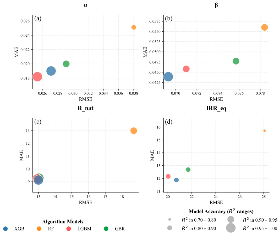
Among the four parameters, the intercept-derived quantities—α and R_nat—are reconstructed with the highest fidelity. The boosting algorithms (XGBoost, LightGBM, and GBR) consistently achieve R² > 0.96 for α (RMSE < 0.030) and R² > 0.96 for R_nat (RMSE ≈ 13 mm yr⁻¹), with XGBoost and LightGBM yielding the lowest errors (Figure 8). The irrigation infiltration coefficient β, which represents the first derivative of the IRR–Recharge function, is predicted with R² ranging from 0.90 to 0.96. This moderate reduction reflects the greater sensitivity of derivative-based quantities to coefficient prediction errors relative to intercept-based ones. Notably, IRR_eq—computed as the positive root of the IRR–Water Table function—is predicted with RMSE of 20–22 mm and MAE of approximately 12 mm by the boosting algorithms, indicating that error propagation through the predicted coefficients remains well-controlled. RF consistently yields higher RMSE and MAE than the boosting family across all five parameters. These results confirm that the gray-box framework can reproduce the key parameters of a full process-based model at a fraction of the computational cost.

A more demanding test is whether the inverted parameters are consistent with independently measured or assessed hydrogeological values—data that were not used in model training. The precipitation infiltration coefficient α has a mean of 0.097 and an interquartile range of 0.053–0.123, consistent with the groundwater resource assessment of the Haihe River basin [59], which reports α values of 0.03–0.20 for sub-clay soils, 0.09–0.24 for sub-sandy soils, and 0.07–0.16 for interbedded sub-sandy and sub-clay soils in the piedmont alluvial–proluvial plain at water-table depths exceeding 6 m—the prevailing condition across the study area. The irrigation infiltration coefficient β has a mean of 0.199 with an interquartile range of 0.093–0.293, broadly consistent with field-based estimates of 0.07–0.23 for sub-clay soils, 0.08–0.26 for sub-sandy soils, and 0.10–0.30 for fine sandy soils under a 75 mm irrigation application depth in this region [48,59]. The natural recharge R_nat averages 70.5 mm yr⁻¹ across the study area as directly inverted from the IRR–Storage function; however, it should be noted that the SWAT-GW simulations include a pre-sowing summer-maize irrigation—sourced from groundwater to ensure germination—that is not accounted for in conventional natural recharge assessments but constitutes a genuine aquifer input. Adding the multi-year average pre-sowing irrigation of approximately 55 mm [11] yields an adjusted R_nat of approximately 125.5 mm yr⁻¹, in good agreement with the independently assessed values of 129 mm yr⁻¹ for the Dianxi Plain of the Daqing River basin and 122 mm yr⁻¹ for the plain of the Ziya River basin [59,60,61]. The recharge–abstraction equilibrium point IRR_eq for winter wheat averages 55.0 mm (central 75%: 24.1–77.1 mm) across the study area. Accounting for the pre-sowing maize irrigation (~45 mm), the total annual groundwater extraction consistent with aquifer equilibrium averages approximately 100 mm However, this scientifically inverted threshold is drastically lower than the current regional agricultural practice, in which 200–300 mm of groundwater is typically pumped for irrigation annually. This massive discrepancy between the sustainable capacity (~100 mm) and the actual extraction (200–300 mm) mathematically confirms the severe and persistent aquifer overdraft, underscoring the urgent need to transition from yield-driven irrigation to sustainable water-saving regimes [11,15]. The spatial distribution of IRR_eq provides a direct, spatially resolved basis for differentiated irrigation quota management without the computational cost of distributed numerical modeling.

The agreement between ML-inverted parameters and independent reference values—obtained from field investigations and regional groundwater assessments entirely external to the model training process—confirms that the gray-box framework captures physically meaningful irrigation–groundwater relationships rather than merely reproducing statistical patterns in the training data.

4.4. SHAP-Based Feature Attribution and Mechanistic Consistency Check

To examine whether the ML models capture physically meaningful relationships rather than spurious statistical patterns, SHAP analysis and Causal Forest were applied to two representative inverted parameters: the recharge–abstraction equilibrium point (IRR_eq) and the irrigation infiltration coefficient (β). The selection of these two parameters reflects a deliberate contrast in physical character. Among the four inverted parameters, precipitation-derived recharge, natural recharge, and IRR_eq form a physically nested hierarchy—precipitation recharge combined with lateral inflow approximates natural recharge, which in turn, combined with irrigation return flow, approximates the recharge–abstraction equilibrium—making IRR_eq the most integrative and management-critical of the three, and the natural endpoint for interpretability analysis. The irrigation infiltration coefficient β, by contrast, is a derivative-based quantity representing the marginal efficiency of human-applied irrigation in generating aquifer recharge—structurally distinct from the intercept-derived natural parameters and uniquely sensitive to anthropogenic management decisions. Examining these two parameters together thus spans both the natural recharge system and the human intervention pathway.

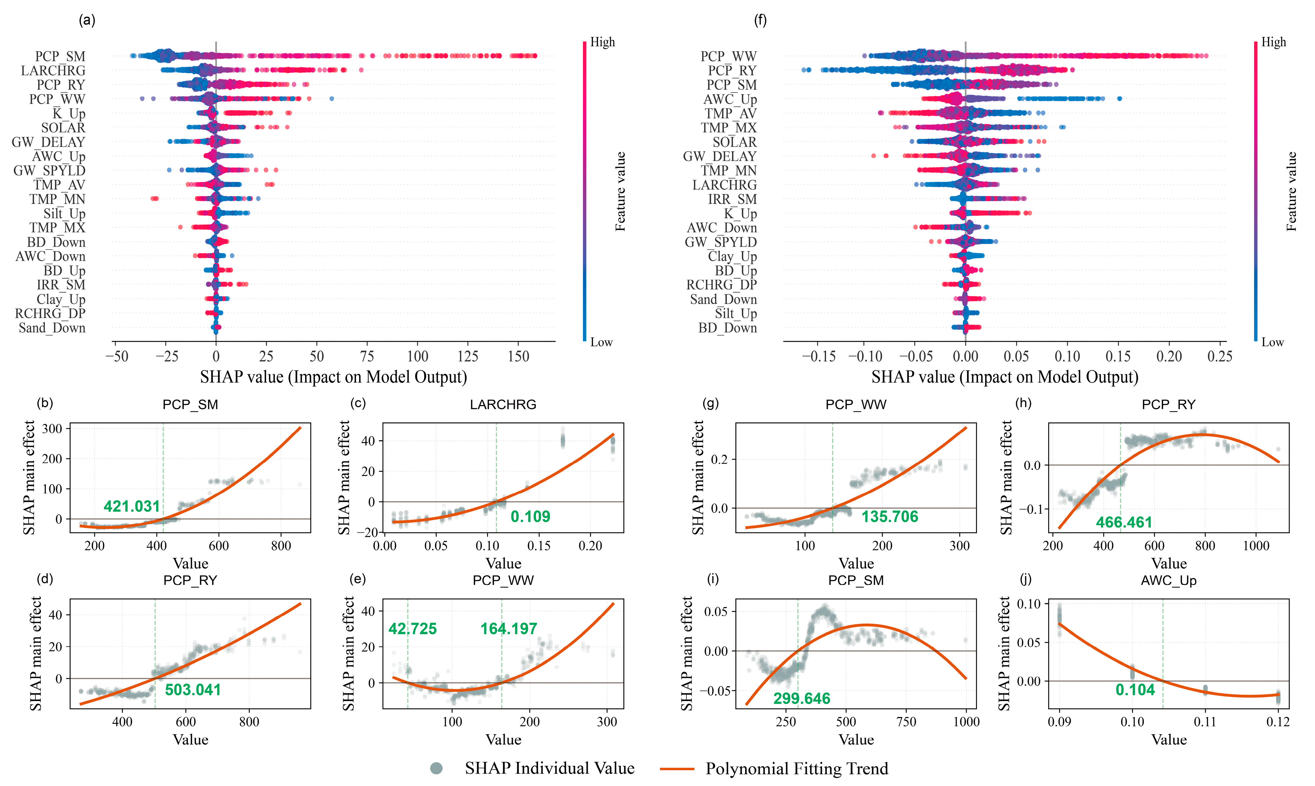
The SHAP global importance rankings (Figure 9a,f) are broadly consistent with physical expectations. For IRR_eq, precipitation variables (PCP_SM, PCP_RY, PCP_WW) and lateral recharge (LARCHRG) collectively dominate, followed by soil hydraulic conductivity (K_Up)—a pattern consistent with the understanding that the recharge–abstraction equilibrium threshold is primarily determined by the combined availability of vertical precipitation-driven recharge and lateral inflow from the adjacent mountains, mediated by the soil’s hydraulic transmissivity. For β, the feature importance structure shifts toward soil properties: available water capacity of the upper layer (AWC_Up) emerges as a prominent negative driver alongside precipitation variables, suggesting that soils with high water retention capacity tend to partition irrigation water toward crop uptake rather than deep percolation—a result physically consistent with vadose-zone water partitioning theory. The SHAP dependence plots (Figure 9b–e,g–j) further suggest threshold-dependent relationships for precipitation variables, where contributions to IRR_eq and β transition from negative to positive above approximate critical levels, though the precise thresholds should be interpreted with caution given the collinearity among seasonal precipitation indices.

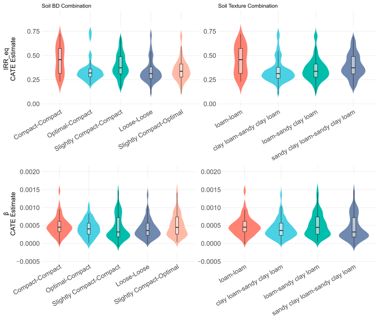
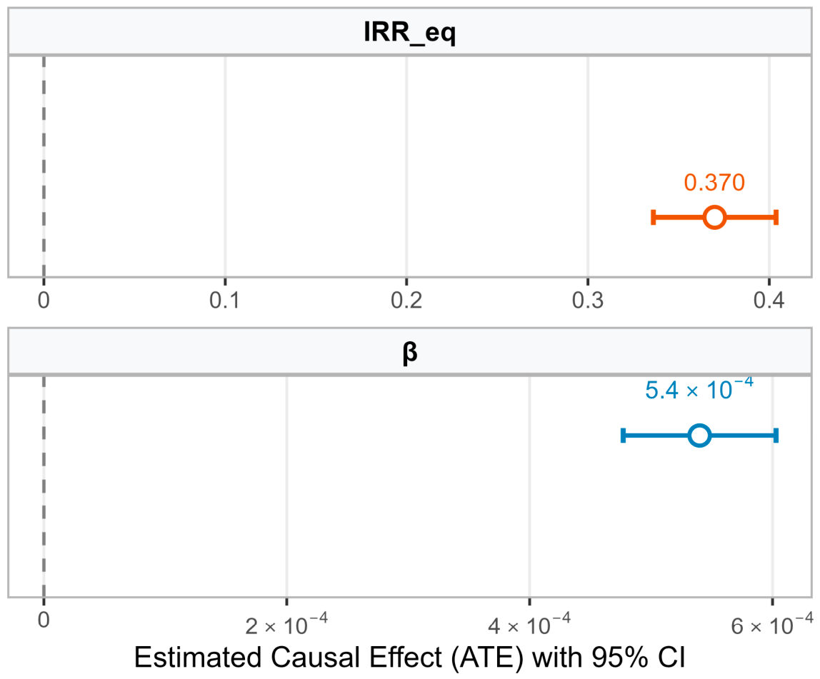
To move beyond association toward causal quantification, a Causal Forest was applied, with annual precipitation (PCP_RY) as a continuous treatment variable. The estimated ATE of precipitation on IRR_eq was 0.369 mm mm⁻¹ (95% CI: 0.336–0.403) and on β was 5.39 × 10⁻⁴ mm⁻¹ (95% CI: 4.77–6.02 × 10⁻⁴), both significantly positive (Figure 10), indicating that precipitation exerts a genuine positive causal effect on both parameters after controlling for soil confounders. The CATE analysis (Figure 11) reveals that this effect is heterogeneous across soil configurations—compact bulk density combinations and loam-dominated texture pairs tend to exhibit higher CATE values for IRR_eq, suggesting that the precipitation sensitivity of the aquifer equilibrium point may be modulated by soil physical properties, though the mechanistic interpretation of this heterogeneity warrants further investigation. Calibration tests confirm statistically significant CATE heterogeneity (IRR_eq: coefficient = 1.23, SE = 0.16, p < 0.001; β: coefficient = 1.53, SE = 0.08, p < 0.001).

Taken together, these analyses rigorously validate the mechanistic consistency of the machine learning model. The convergence between SHAP-identified feature hierarchies—where precipitation and lateral recharge correctly emerge as the dominant drivers of IRR_eq—and established hydrogeological theory provides strong evidence that the gray-box ML framework has learned physically grounded relationships rather than mere statistical artifacts. Furthermore, the Causal Forest confirms that precipitation exerts a genuine positive causal effect on aquifer sustainability metrics, responding to climate forcing in a physically interpretable direction. This alignment between data-driven algorithms and physical mechanics lends substantial credibility to their use in evidence-based groundwater management.

5. Discussion

5.1. Physical Interpretability of the Quadratic Response Framework

The central methodological contribution of this study is the use of low-order polynomial coefficients (a, b, c)—rather than state variables—as the ML learning target. This design transforms the ML output from an opaque numerical prediction into a compact, physically structured representation of the irrigation–groundwater relationship, enabling reconstruction of the groundwater response at any irrigation intensity and direct comparison across spatial units.

The rationale rests on the well-established moisture-dependent nature of soil water infiltration and redistribution. Under the frameworks of the Green–Ampt and Richards equations, infiltration rate is not constant but varies with antecedent moisture content—drier soils resist percolation, while wetter soils transmit water more readily until approaching saturation, at which point infiltration converges toward the saturated hydraulic conductivity [62,63]. When irrigation intensity serves as the independent variable, increasing irrigation progressively wets the soil profile, accelerating percolation at low-to-moderate intensities but yielding diminishing marginal gains as the profile approaches field capacity and saturation. This concave-upward behavior for Recharge, and the corresponding concave-downward behavior for Storage and Water Table—where pumping increasingly outpaces the decelerating recharge gains—are functional shapes inherently consistent with a second-order polynomial. The linear form, by contrast, cannot represent this moisture-dependent curvature, as evidenced by its systematic underestimation of recharge under rain-fed conditions and its inability to capture the flattening of Storage and Water Table responses at high irrigation intensities (Section 4.1, Figure 4).

The cubic form offers only marginal improvement in fitting accuracy while introducing a leading coefficient on the order of 10⁻⁵ to 10⁻⁷ that proves poorly learnable by ML algorithms (Section 4.1). At the annual and HRU spatial scale adopted in this study, the dominant nonlinearity in the irrigation–groundwater pathway is adequately captured by a single curvature parameter. Whether finer temporal resolutions (e.g., event-based or seasonal) or more heterogeneous hydrogeological settings would necessitate higher-order representations remains to be explored in future work.

5.2. Methodological Positioning and Practical Implications

The gray-box framework occupies a distinct position within the broader landscape of physics-informed machine learning [19,23]. By learning functional coefficients rather than state variables, it shifts the ML objective from descriptive prediction—forecasting what the groundwater state will be under certain given conditions—toward prescriptive inference—determining how irrigation should be managed to achieve a desired aquifer outcome. This distinction carries direct practical significance, as the learned coefficients yield, through analytical operations on the fitted function (Section 3.2), the management-critical parameters (α, β, R_nat, IRR_eq) that conventional black-box ML approaches cannot provide [20,22].

Relative to existing PIML strategies, the proposed gray-box polynomial-coefficient framework addresses a different scale and objective. PINNs have achieved remarkable success in fine-scale subsurface characterization—coupling governing equations such as Darcy’s law and the Richards equation into neural network training to estimate spatially heterogeneous hydraulic parameters and discover constitutive relationships from sparse observations [24,25,26]. These studies resolve individual physical processes at spatial scales ranging from laboratory columns to small catchments. The proposed framework does not attempt this level of process resolution; instead, it operates at the integrated crop–soil–groundwater system level, where the focus shifts from solving flow equations to capturing the aggregate response of the coupled agricultural-hydrological system to irrigation management. ML surrogate models have likewise proven effective at emulating high-dimensional spatiotemporal outputs of numerical simulators for accelerated scenario analysis and parameter inversion [27,28]. The proposed framework complements these approaches by reducing the emulation target to a low-dimensional coefficient vector that is directly interpretable in hydrogeological terms. Each strategy serves a distinct purpose: PINNs and surrogates excel at detailed process characterization and high-resolution state emulation, while the gray-box framework is oriented toward regional-scale management inference, for which explicit irrigation–groundwater functional relationships are the primary deliverable.

The proposed framework does require a well-calibrated process-based model as the training data generator. This prerequisite is increasingly attainable in practice, as most major over-exploited aquifer systems—including the Indo-Gangetic Plains, the U.S. High Plains, and the Murray–Darling Basin—now have operational agro-hydrological models supported by decades of monitoring infrastructure [12,14,64]. The gray-box framework offers a pathway for distilling the outputs of such existing models into compact, interpretable functional representations that can serve as rapid decision-support tools for irrigation-driven groundwater management.

Building on these decision-support capabilities, the framework provides a direct quantitative foundation for enacting targeted policies and guidelines for groundwater mitigation and adaptation in the study region. As emphasized in the recent literature [65], effective water governance must center policymaking around divergent regional factors. Our methodology facilitates this by explicitly highlighting the importance of variability across different spatiotemporal scales and various agricultural communities. Rather than relying on a “one-size-fits-all” approach, water managers can utilize the spatially heterogeneous IRR_eq values to design community-specific guidelines. For instance, dynamic adaptation strategies can be deployed in resilient localities, whereas in severely depleted communities, the inverted IRR_eq provides a strict, quantitative baseline for mitigation policies, such as establishing precision pumping quotas.

5.3. Limitations and Future Directions

The applicability boundaries and data requirements of the framework deserve careful consideration. The feature ablation analysis (Section 4.2) demonstrates that the IRR–Recharge and IRR–Storage coefficients can be predicted with acceptable accuracy using meteorological and basic soil data alone, while the SHAP and Causal Forest analyses (Section 4.4) reveal that IRR_eq is most sensitive to precipitation, lateral recharge, and soil hydraulic conductivity. Synthesizing these findings provides layered guidance for data-limited applications: in regions where only meteorological and soil texture data are available, the framework can reliably estimate the precipitation infiltration coefficient (α) and approximate the irrigation–recharge relationship; obtaining the recharge–abstraction equilibrium point (IRR_eq) with higher confidence requires, in addition, estimates of lateral recharge and soil hydraulic conductivity—parameters that can often be approximated from regional groundwater resource assessments and pedotransfer functions; specific yield (GW_SPYLD), while critical for the IRR–Water Table pathway, can be partially circumvented by deriving IRR_eq from the more robust IRR–Storage pathway.

Several scope-related limitations should be noted. The quadratic approximation has been developed and validated for a piedmont alluvial plain with relatively homogeneous Quaternary pore aquifers under flood irrigation conditions. Its applicability to hydrogeological settings with fundamentally different flow regimes—such as karst conduit systems, fractured rock aquifers, or shallow water-table areas with strong groundwater–surface water exchange—would require separate evaluation. Specifically, the smooth and continuous nature of quadratic functions may fail to capture the abrupt, threshold-triggered preferential flows typical of karst and fractured systems. Similarly, strong bidirectional groundwater–surface water interactions or shallow phreatic evaporation can introduce buffering effects, leading to piecewise or asymptotic responses rather than continuous polynomial trends. Consequently, under such conditions, the irrigation–groundwater pathway exhibits qualitatively different nonlinear behaviors that would necessitate alternative functional forms (e.g., threshold or piecewise functions) or hybrid model architecture. The framework currently operates at an annual time scale, capturing the long-term average response rather than within-season dynamics or interannual transient behavior; extending the approach to seasonal resolution would require sub-annual polynomial fitting or hybrid architectures combining functional coefficients with temporal sequence models. The training data are generated by the SWAT-GW model, which serves as an effective bridge for producing the large-sample paired datasets that field experiments alone cannot provide, and has been rigorously calibrated and validated against multiple independent data sources [11,43]. Nonetheless, the model necessarily simplifies certain subsurface processes at sub-HRU scales, and these simplifications propagate into the ML-learned coefficients; incorporating field-measured irrigation–recharge pairs, where available, would further strengthen the physical credibility of the framework. Finally, under evolving climate conditions, the response function coefficients themselves may shift as precipitation regimes and crop-water demand change; the temporal stability of the learned relationships should be evaluated through multi-period retraining or climate-scenario ensemble experiments.

6. Conclusions

This study developed a gray-box machine learning framework in which the learning target is shifted from groundwater state variables to the parametric coefficients of quadratic response functions linking irrigation intensity to three key groundwater variables—recharge, aquifer storage change, and water table depth change. Applied to the piedmont plain of the Taihang Mountains in the North China Plain, the methodology explicitly extracts invertible hydrogeological parameters from process-based SWAT-GW model outputs, advancing groundwater machine learning beyond state prediction and toward quantitative, management-relevant inference for over-exploited aquifer systems.

The principal findings demonstrate that quadratic polynomials optimally balance fitting accuracy ($R^2>0.994$), machine learning learnability, and physical interpretability. From the learned coefficients, four management-critical parameters, namely, the precipitation infiltration coefficient ($\alpha$), the irrigation infiltration coefficient ($\beta$), natural recharge (R_nat), and a recharge–abstraction equilibrium point (IRR_eq), were successfully inverted and validated against independent assessments. Furthermore, the framework exhibited physically interpretable robustness under data scarcity, with feature sensitivities—such as the dependence on specific yield for water table predictions—aligning perfectly with SHAP attributions and established hydrogeological understanding. Despite these promising outcomes, several scope-related limitations remain. The current quadratic approximation is validated for relatively homogeneous alluvial plains at an annual scale; its application to complex karst or fractured aquifers with threshold-triggered preferential flows would necessitate alternative functional architectures. Additionally, the framework currently relies on simulated training datasets. Future research should focus on extending this approach to sub-annual resolutions while using hybrid temporal models, incorporating field-measured paired datasets to further validate the learned relationships, and assessing the temporal stability of the response coefficients under evolving climate scenarios.

References

1. Siebert, S.; Burke, J.; Faures, J.M.; Frenken, K.; Hoogeveen, J.; Döll, P.; Portmann, F.T. Groundwater Use for Irrigation—A Global Inventory. Hydrol. Earth Syst. Sci. 2010, 14, 1863–1880. [Google Scholar] [CrossRef]
2. FAO. The State of the World’s Land and Water Resources for Food and Agriculture (SOLAW): Managing Systems at Risk, 1st ed.; The State of the World’s Land and Water Resources for Food and Agriculture; FAO and Earthscan from Routledge: Rome, Italy, 2011. [Google Scholar]
3. Bierkens, M.F.P.; Wada, Y. Non-Renewable Groundwater Use and Groundwater Depletion: A Review. Environ. Res. Lett. 2019, 14, 063002. [Google Scholar] [CrossRef]
4. United Nations. The United Nations World Water Development Report 2022: Groundwater: Making the Invisible Visible; UNESCO: Paris, France, 2022. [Google Scholar]
5. Abhishek; Kinouchi, T. Synergetic Application of GRACE Gravity Data, Global Hydrological Model, and in-Situ Observations to Quantify Water Storage Dynamics over Peninsular India during 2002–2017. J. Hydrol. 2021, 596, 126069. [Google Scholar] [CrossRef]
6. Rodell, M.; Velicogna, I.; Famiglietti, J.S. Satellite-Based Estimates of Groundwater Depletion in India. Nature 2009, 460, 999–1002. [Google Scholar] [CrossRef] [PubMed]
7. Zheng, C.; Liu, J.; Cao, G.; Kendy, E.; Wang, H.; Jia, Y. Can China Cope with Its Water Crisis?—Perspectives from the North China Plain. Groundwater 2010, 48, 350–354. [Google Scholar] [CrossRef] [PubMed]
8. Scanlon, B.R.; Faunt, C.C.; Longuevergne, L.; Reedy, R.C.; Alley, W.M.; McGuire, V.L.; McMahon, P.B. Groundwater Depletion and Sustainability of Irrigation in the US High Plains and Central Valley. Proc. Natl. Acad. Sci. USA 2012, 109, 9320–9325. [Google Scholar] [CrossRef] [PubMed]
9. Wada, Y.; van Beek, L.P.H.; Bierkens, M.F.P. Nonsustainable Groundwater Sustaining Irrigation: A Global Assessment. Water Resour. Res. 2012, 48, W00L06. [Google Scholar] [CrossRef]
10. Döll, P.; Müller Schmied, H.; Schuh, C.; Portmann, F.T.; Eicker, A. Global-Scale Assessment of Groundwater Depletion and Related Groundwater Abstractions: Combining Hydrological Modeling with Information from Well Observations and GRACE Satellites. Water Resour. Res. 2014, 50, 5698–5720. [Google Scholar] [CrossRef]
11. Zhang, X.; Ren, L.; Kong, X. Estimating Spatiotemporal Variability and Sustainability of Shallow Groundwater in a Well-Irrigated Plain of the Haihe River Basin Using SWAT Model. J. Hydrol. 2016, 541, 1221–1240. [Google Scholar] [CrossRef]
12. Bailey, R.T.; Wible, T.C.; Arabi, M.; Records, R.M.; Ditty, J. Assessing Regional-scale Spatio-temporal Patterns of Groundwater–Surface Water Interactions Using a Coupled SWAT-MODFLOW Model. Hydrol. Process. 2016, 30, 4420–4433. [Google Scholar] [CrossRef]
13. Liu, M.; Jiang, Y.; Xu, X.; Huang, Q.; Huo, Z.; Huang, G. Long-Term Groundwater Dynamics Affected by Intense Agricultural Activities in Oasis Areas of Arid Inland River Basins, Northwest China. Agric. Water Manag. 2018, 203, 37–52. [Google Scholar] [CrossRef]
14. Zhu, J.; Zhang, X.; Chen, Y. Development and Testing of an Integrated APEX-SWAT-GW Model for Simulations of Agro-Hydrological Processes in a Groundwater-Fed Plain in China. Environ. Model. Softw. 2023, 168, 105804. [Google Scholar] [CrossRef]
15. Zhang, X.; Ren, L.; Wan, L. Assessing the Trade-off between Shallow Groundwater Conservation and Crop Production under Limited Exploitation in a Well-Irrigated Plain of the Haihe River Basin Using the SWAT Model. J. Hydrol. 2018, 567, 253–266. [Google Scholar] [CrossRef]
16. Zhang, X.; Ren, L. Simulating and Assessing the Effects of Seasonal Fallow Schemes on the Water-Food-Energy Nexus in a Shallow Groundwater-Fed Plain of the Haihe River Basin of China. J. Hydrol. 2021, 595, 125992. [Google Scholar] [CrossRef]
17. Ou, J.; Ding, B.; Feng, P.; Chen, Y.; Yu, L.; Liu, D.L.; Srinivasan, R.; Zhang, X. How to Stop Groundwater Drawdown in North China Plain? Combining Agricultural Management Strategies and Climate Change. J. Hydrol. 2025, 647, 132352. [Google Scholar] [CrossRef]
18. Barthel, R.; Banzhaf, S. Groundwater and Surface Water Interaction at the Regional-Scale—A Review with Focus on Regional Integrated Models. Water Resour. Manag. 2016, 30, 1–32. [Google Scholar] [CrossRef]
19. Shen, C.; Appling, A.P.; Gentine, P.; Bandai, T.; Gupta, H.; Tartakovsky, A.; Baity-Jesi, M.; Fenicia, F.; Kifer, D.; Li, L.; et al. Differentiable Modelling to Unify Machine Learning and Physical Models for Geosciences. Nat. Rev. Earth Environ. 2023, 4, 552–567. [Google Scholar] [CrossRef]
20. Tao, H.; Hameed, M.M.; Marhoon, H.A.; Zounemat-Kermani, M.; Heddam, S.; Kim, S.; Sulaiman, S.O.; Tan, M.L.; Sa’adi, Z.; Mehr, A.D.; et al. Groundwater Level Prediction Using Machine Learning Models: A Comprehensive Review. Neurocomputing 2022, 489, 271–308. [Google Scholar] [CrossRef]
21. Zhang, J.; Zhu, Y.; Zhang, X.; Ye, M.; Yang, J. Developing a Long Short-Term Memory (LSTM) Based Model for Predicting Water Table Depth in Agricultural Areas. J. Hydrol. 2018, 561, 918–929. [Google Scholar] [CrossRef]
22. Cai, H.; Shi, H.; Zhou, Z.; Liu, S.; Babovic, V. Explaining the Mechanism of Multiscale Groundwater Drought Events: A New Perspective from Interpretable Deep Learning Model. Water Resour. Res. 2024, 60, e2023WR035139. [Google Scholar] [CrossRef]
23. Reichstein, M.; Camps-Valls, G.; Stevens, B.; Jung, M.; Denzler, J.; Carvalhais, N.; Prabhat, F. Deep Learning and Process Understanding for Data-Driven Earth System Science. Nature 2019, 566, 195–204. [Google Scholar] [CrossRef] [PubMed]
24. Tartakovsky, A.M.; Marrero, C.O.; Perdikaris, P.; Tartakovsky, G.D.; Barajas-Solano, D. Physics-Informed Deep Neural Networks for Learning Parameters and Constitutive Relationships in Subsurface Flow Problems. Water Resour. Res. 2020, 56, e2019WR026731. [Google Scholar] [CrossRef]
25. Song, W.; Shi, L.; Wang, L.; Wang, Y.; Hu, X. Data-Driven Discovery of Soil Moisture Flow Governing Equation: A Sparse Regression Framework. Water Resour. Res. 2022, 58, e2022WR031926. [Google Scholar] [CrossRef]
26. He, L.; Shi, L.; Song, W.; Shen, J.; Wang, L.; Hu, X.; Zha, Y. Synergizing Intuitive Physics and Big Data in Deep Learning: Can We Obtain Process Insights While Maintaining State-of-the-Art Hydrological Prediction Capability? Water Resour. Res. 2024, 60, e2024WR037582. [Google Scholar] [CrossRef]
27. Razavi, S.; Tolson, B.A.; Burn, D.H. Review of Surrogate Modeling in Water Resources. Water Resour. Res. 2012, 48, W07401. [Google Scholar] [CrossRef]
28. Dai, T.; Maher, K.; Perzan, Z. Machine Learning Surrogates for Efficient Hydrologic Modeling: Insights from Stochastic Simulations of Managed Aquifer Recharge. J. Hydrol. 2025, 652, 132606. [Google Scholar] [CrossRef]
29. Scanlon, B.R.; Healy, R.W.; Cook, P.G. Choosing Appropriate Techniques for Quantifying Groundwater Recharge. Hydrogeol. J. 2002, 10, 18–39. [Google Scholar] [CrossRef]
30. Healy, R.W.; Scanlon, B.R. Estimating Groundwater Recharge; Cambridge University Press: Cambridge, UK, 2010. [Google Scholar]
31. Foster, S.; Garduno, H.; Evans, R.; Olson, D.; Tian, Y.; Zhang, W.; Han, Z. Quaternary Aquifer of the North China Plain—Assessing and Achieving Groundwater Resource Sustainability. Hydrogeol. J. 2004, 12, 81–93. [Google Scholar] [CrossRef]
32. De Vries, J.J.; Simmers, I. Groundwater Recharge: An Overview of Processes and Challenges. Hydrogeol. J. 2002, 10, 5–17. [Google Scholar] [CrossRef]
33. Gleeson, T.; Wada, Y.; Bierkens, M.F.P.; van Beek, L.P.H. Water Balance of Global Aquifers Revealed by Groundwater Footprint. Nature 2012, 488, 197–200. [Google Scholar] [CrossRef] [PubMed]
34. Sophocleous, M. From Safe Yield to Sustainable Development of Water Resources—The Kansas Experience. J. Hydrol. 2000, 235, 27–43. [Google Scholar] [CrossRef]
35. Han, P. Status quo of Groundwater Development and Utilization in Haihe River Basin and its Management. Haihe Water Resour. 2015, 1, 1–5. (In Chinese) [Google Scholar] [CrossRef]
36. Liu, C. Discussion on Some Problems of China’s Water Resources in 21st Century. Water Resour. Hydropower Eng. 2002, 33, 15–19. (In Chinese) [Google Scholar] [CrossRef]
37. Jia, X.; Hou, D.; Wang, L.; O’Connor, D.; Luo, J. The Development of Groundwater Research in the Past 40 Years: A Burgeoning Trend in Groundwater Depletion and Sustainable Management. J. Hydrol. 2020, 587, 125006. [Google Scholar] [CrossRef]
38. The People’s Government of Hebei Province. Pilot Project of Comprehensive Treatment on Groundwater Over-Exploitation in Hebei Province in 2014. Available online: https://www.hebei.gov.cn/columns/43e11810-5806-4099-84ab-0c9bc150e7d6/202309/11/5149385c-1420-4f81-bc61-2f93cd797d3b.html (accessed on 4 May 2026). (In Chinese)
39. The State Council Information Office. The State Council Information Office Held a Press Conference on the Progress and Effectiveness of National Water Security. Available online: https://www.gov.cn/lianbo/fabu/202403/content_6939915.htm (accessed on 4 May 2026). (In Chinese)
40. Long, D.; Xu, Y.; Cui, Y.; Cui, Y.; Butler, J.J.; Dong, L.; Wang, L.; Liu, D.; Wada, Y.; Hu, L.; et al. Unprecedented Large-Scale Aquifer Recovery through Human Intervention. Nat. Commun. 2025, 16, 7296. [Google Scholar] [CrossRef] [PubMed]
41. Zhang, X.; Ding, B.; Hou, Y.; Feng, P.; Liu, D.L.; Srinivasan, R.; Chen, Y. Assessing the Feasibility of Sprinkler Irrigation Schemes and Their Adaptation to Future Climate Change in Groundwater Over-Exploitation Regions. Agric. Water Manag. 2024, 292, 108674. [Google Scholar] [CrossRef]
42. Wang, B.G.; Jin, M.G.; Nimmo, J.R.; Yang, L.; Wang, W.F. Estimating groundwater recharge in Hebei plain, China under varying land use practices using tritium and bromide tracers. J. Hydrol. 2008, 356, 209–222. [Google Scholar] [CrossRef]
43. Zhang, X.; Ren, L.; Feng, W. Comparison of the Shallow Groundwater Storage Change Estimated by a Distributed Hydrological Model and GRACE Satellite Gravimetry in a Well-Irrigated Plain of the Haihe River Basin, China. J. Hydrol. 2022, 610, 127799. [Google Scholar] [CrossRef]
44. Mehdinejadiani, B. A Novel Inverse Model Insensitive to Initial Guesses for Estimating Parameters of Continuous Time Random Walk-Truncated Power Law Model. J. Hydrol. 2025, 658, 133206. [Google Scholar] [CrossRef]
45. Marino, S.; Hogue, I.B.; Ray, C.J.; Kirschner, D.E. A Methodology for Performing Global Uncertainty and Sensitivity Analysis in Systems Biology. J. Theor. Biol. 2008, 254, 178–196. [Google Scholar] [CrossRef] [PubMed]
46. Shen, Z.R.; Wang, L.; Yu, F.L.; Liu, B. New Concept of Water Saving-Study and Application of Real Water Saving; China Water Power Press: Beijing, China, 2000. [Google Scholar]
47. Zhang, X.; Ren, L.; Zhao, J. Economic Approach for Optimal Allocation of Irrigation Water in Water-Scarce Region. Agric. Water Manag. 2025, 317, 109630. [Google Scholar] [CrossRef]
48. China Geological Survey (CGS). Investigation and Assessment of Groundwater Sustainable Utilization in the North China Plain; Geological Publishing House: Beijing, China, 2009. (In Chinese)
49. Breiman, L. Random Forests. Mach. Learn. 2001, 45, 5–32. [Google Scholar] [CrossRef]
50. Friedman, J.H. Greedy Function Approximation: A Gradient Boosting Machine. Ann. Stat. 2001, 29, 1189–1232. [Google Scholar] [CrossRef]
51. Chen, T.; Guestrin, C. XGBoost: A Scalable Tree Boosting System. In Proceedings of the 22nd ACM SIGKDD International Conference on Knowledge Discovery and Data Mining; ACM: San Francisco, CA, USA, 2016; pp. 785–794. [Google Scholar]
52. Ke, G.; Meng, Q.; Finley, T.; Wang, T.; Chen, W.; Ma, W.; Ye, Q.; Liu, T.-Y. Lightgbm: A Highly Efficient Gradient Boosting Decision Tree. In Proceedings of the 31st Conference on Neural Information Processing Systems (NIPS 2017), Long Beach, CA, USA, 4–9 December 2017; Volume 30. [Google Scholar]
53. Snoek, J.; Larochelle, H.; Adams, R.P. Practical Bayesian Optimization of Machine Learning Algorithms. Adv. Neural Inf. Process. Syst. 2012, 25, 2951–2959. [Google Scholar]
54. Lundberg, S.; Lee, S.-I. A Unified Approach to Interpreting Model Predictions 2017. In Proceedings of the 31st International Conference on Neural Information Processing Systems, Long Beach, CA, USA, 4–9 December 2017. [Google Scholar]
55. Athey, S.; Tibshirani, J.; Wager, S. Generalized Random Forests. Ann. Stat. 2019, 42, 1148–1178. [Google Scholar] [CrossRef]
56. Wager, S.; Athey, S. Estimation and Inference of Heterogeneous Treatment Effects Using Random Forests. J. Am. Stat. Assoc. 2018, 113, 1228–1242. [Google Scholar] [CrossRef]
57. Tibshirani, J.; Athey, S.; Friedberg, R.; Hadad, V.; Hirshberg, D.; Miner, L.; Sverdrup, E.; Wager, S.; Wright, M. Grf: Generalized Random Forests. 2025. Available online: https://cran.r-project.org/web/packages/grf/index.html (accessed on 4 May 2026).
58. Mehdinejadiani, B.; Fathi, P. Analytical Solutions of Space Fractional Boussinesq Equation to Simulate Water Table Profiles between Two Parallel Drainpipes under Different Initial Conditions. Agric. Water Manag. 2020, 240, 106324. [Google Scholar] [CrossRef]
59. Ren, X. Assessment of Groundwater Resources in the Haihe River Basin; Water & Power Press: Beijing, China, 2007. (In Chinese) [Google Scholar]
60. Zhang, Z.; Li, L. Groundwater Resources of China-Hebei Volume; Sinomaps Press: Beijing, China, 2005. (In Chinese) [Google Scholar]
61. National Groundwater Resources; Assessment Project Office Attached Tables of National Groundwater Resources Assessment. National Groundwater Resources: Beijing, China, 2004; unpublished. (In Chinese)
62. Herber Green, W.; Ampt, G.A. Studies of Soil Physics I. The Flow of Air and Water through Soils. J. Agric. Sci. 1911, 4, 11–24. [Google Scholar] [CrossRef]
63. Assouline, S. Infiltration into Soils: Conceptual Approaches and Solutions. Water Resour. Res. 2013, 49, 1755–1772. [Google Scholar] [CrossRef]
64. Steward, D.R.; Bruss, P.J.; Yang, X.; Staggenborg, S.A.; Welch, S.M.; Apley, M.D. Tapping Unsustainable Groundwater Stores for Agricultural Production in the High Plains Aquifer of Kansas, Projections to 2110. Proc. Natl. Acad. Sci. USA 2013, 110, E3477–E3486. [Google Scholar] [CrossRef] [PubMed]
65. Anjaneyulu, R.; Abhishek. On the Evaluation of Global Terrestrial Water Storage and Divergent Governing Factors Centring Policymaking. J. Environ. Manag. 2026, 398, 128455. [Google Scholar] [CrossRef] [PubMed]
Figure 1. Location map of the study area, subbasins, HURs, and calibration and validation wells for SWAT-GW model.
Water 18 01661 g001
Figure 2. Scatter plot of observed versus simulated shallow groundwater table dynamics for the SWAT-GW model calibration. Note—DXP: Dianxi Plain of the Daqing River basin, ZYHP: the plain of the Ziya River basin.
Water 18 01661 g002
Figure 3. Flow chart of the data processing, machine learning model training, and interpretability and causal inference in this study.
Water 18 01661 g003
Figure 4. Polynomial response function fitting for the three irrigation–groundwater relationships: (A) fitted linear, quadratic, and cubic curves for IRR–Recharge (top row), IRR–Storage (middle row), and IRR–Water Table (bottom row) for a representative HRU, with 95% confidence and prediction bands; (B) probability density distributions of fitted polynomial coefficients across all 70 HRUs for each functional form. The lowercase letters on the y-axis denote the coefficients of the polynomial terms in descending order: in the Linear column, a and b represent the linear and constant terms, respectively; in the Quadratic column, a, b, and c represent the quadratic, linear, and constant terms; in the Cubic column, a, b, c, and d represent the cubic, quadratic, linear, and constant terms.
Water 18 01661 g004
Figure 5. Test-set R2 of the four ensemble ML algorithms for each polynomial coefficient across three response variables and three polynomial orders. On the y-axis, the primary labels indicate the polynomial function type, while the secondary lowercase letters denote the specific mathematical coefficients being predicted. Specifically: under the Linear category ( y = a x + b ), a and b represent the first-order coefficient and the constant term, respectively; under the Quadratic category ( y = a x 2 + b x + c ), a, b, and c represent the second-order coefficient, first-order coefficient, and constant term, respectively; under the Cubic category ( y = a x 3 + b x 2 + c x + d ), a, b, c, and d represent the third-order, second-order, first-order coefficients, and the constant term, respectively.
Water 18 01661 g005
Figure 6. Test-set R2 of the four ensemble ML algorithms, for each quadratic coefficient (a, b, c) of the three response variables (Recharge, Storage, and Water Table) under three feature availability scenarios: Base (full feature set), Mid (Tier 1 + 2), and Extreme (Tier 1 only).
Water 18 01661 g006
Figure 7. Permutation importance of the top-ranked input features for each polynomial coefficient (outputs a, b, c) of the three response variables (Recharge, Storage, and Water Table) across the four ensemble ML algorithms, based on the full feature set (Tier 1 + 2 + 3).
Water 18 01661 g007
Figure 8. Accuracy of ML-inverted hydrogeological parameters against SWAT-GW benchmark values: (a) precipitation infiltration coefficient α, (b) irrigation infiltration coefficient β, (c) natural recharge R_nat, and (d) recharge–abstraction equilibrium point IRR_eq. Bubble size indicates R2 range; axes show RMSE and MAE for each algorithm.
Water 18 01661 g008
Figure 9. SHAP-based feature attribution for the recharge–abstraction equilibrium point (IRR_eq) and the irrigation infiltration coefficient (β): (a,f) global feature importance summary plots; (be) SHAP main effect partial dependence plots for the top four predictors of IRR_eq; (gj) corresponding plots for the top four predictors of β. Color indicates normalized feature value (red: high; blue: low).
Water 18 01661 g009
Figure 10. Estimated average treatment effects (ATEs) of annual precipitation (PCP_RY) on the recharge–abstraction equilibrium point (IRR_eq) and the irrigation infiltration coefficient (β), with 95% confidence intervals.
Water 18 01661 g010
Figure 11. Conditional average treatment effects (CATEs) of annual precipitation on IRR_eq and β, stratified by soil bulk density combinations and soil texture combinations; classification criteria for each category are provided in Tables S4 and S5.
Water 18 01661 g011