Article

Cumulative Drawdown as a Primary State Variable: The Absement Method for Leaky-Aquifer Pumping-Test Analysis


Department of Civil Engineering, Boğaziçi University, 34340 Istanbul, Türkiye
Water 2026, 18(13), 1638; https://doi.org/10.3390/w18131638
Submission received: 24 May 2026 / Revised: 26 June 2026 / Accepted: 29 June 2026 / Published: 6 July 2026
(This article belongs to the Section Hydrogeology)

Abstract

This study extends the Absement Method to leaky-aquifer pumping-test analysis by time integrating the Hantush–Jacob governing equation and deriving four complementary operators. Time integrating the Hantush–Jacob equation yields S·s = T2AC·A, with storativity S, drawdown s, transmissivity T, the time (t)-integrated drawdown A(t) (absement), and leakance C. The four operators, A(t), time-averaged A(t)/t, windowed ΔAt, and the normalized absement derivative (NAD), are applied jointly across all available observation wells. In a homogeneous aquifer, the fitted operators and NAD diagnostic provide mutually consistent parameter and flow-regime signatures. In a heterogeneous aquifer, systematic differences between operators become part of the interpretation: T-related variation appears as changes in the ΔAt sliding profile across wells, whereas the leakage factor B = √(T/C)-related variation is identified by divergent A(t)/t asymptotes and NAD type-curve crossing. Monte Carlo assessment under composite noise (N = 50) confirms near-zero parameter bias, with T and S standard deviations approximately 3–4 times smaller for A(t)/t and ΔAt than for A(t). The three field cases are identified: a 14% outward T decline with spatially uniform B (sandstone aquifer); approximately homogeneous T with outward-declining B flagged by NAD type-curve crossing before fitting (sandy aquifer); and TB coupling resolution through the windowed ΔAt profile (medium-grained sandstone aquifer). The outputs supported sustainable-yield assessment directly from routine pumping-test records.

1. Introduction

Reliable estimates of transmissivity, storativity, and leakage factor are central to sustainable groundwater management, governing yield, well spacing, and long-term drawdown prediction [1,2]. Leaky aquifers, in which a confined aquifer receives vertical flux through a semi-confining layer, are a common departure from the ideal Theis conditions [3]. Transient solutions were developed by Hantush and Jacob [4,5] and later refined for aquitard storage [6] and two-aquifer flow [7,8], with comprehensive accounts in Kruseman and de Ridder [1], Batu [9], Walton [10], and Woessner et al. [2], and a review by Dashti et al. [11]. Standard interpretation operates on drawdown or its log-derivative: Hantush–Jacob type-curve matching [1,4,5] on s(t), with moderate noise sensitivity; or the inflection-point method [5] and derivative diagnostic plots [12] on ds/d(ln t), which amplify measurement noise by construction, though logarithmic windowing partly mitigates it.
These methods assume spatial homogeneity of transmissivity and leakance, yet both vary in practice, so apparent parameters shift as the cone of depression expands through heterogeneous material. Barker and Herbert [13], Butler [14], and Butler and Liu [15] developed analytical frameworks for non-uniform aquifers, showing that T estimates are spatially averaged quantities whose integration area grows with time, making T more immune to local heterogeneity than S and increasingly representative of broadscale properties at late time, a behavior Manewell et al. [16] linked to regional model parameters. Copty et al. [17] bounded effective transmissivity in a heterogeneous leaky aquifer between the harmonic and geometric means within the leakage radius (≈1.5–2B). Trinchero et al. [18] introduced the double inflection-point technique, which Copty et al. [19] extended stochastically, showing that different methods weight different segments of the record and that aquifer and aquitard heterogeneities leave structurally distinct signatures. More recently, Zhuang et al. [20,21,22] linked anomalous drawdown signatures to vertical aquitard structure, Meng et al. [23] showed that non-Darcian flow in low-permeability aquitards can substantially alter leaky behavior, De Smedt [24] found that aquitard storage is routinely underestimated, and van Leer et al. [25] showed that B confidence intervals widen when the test is shorter than the leakage timescale.
Most methods operate in the drawdown domain, analyzing each observation well separately rather than jointly across the wells of a single pumping test. Time integration has appeared before, but not as a routine diagnostic: Li et al. [26] and Zhu and Yeh [27] used temporal moments as summary statistics for hydraulic tomography, and in petroleum well-testing, the pressure-integral [28] and rate-integral and material-balance-time functions [29] integrate to smooth noise within the conventional drawdown framework rather than reformulating the governing equation around cumulative drawdown. The Incremental Area Method (IAM) of Avcı et al. [30] integrated drawdown sections graphically but lacked a governing equation and a closed-form kernel. Avcı [31] resolved these limitations by time integrating the Theis equation to obtain S · s   =   T 2 A with storativity S, drawdown s, transmissivity T, and the time (t)-integrated drawdown A(t) (absement), establishing absement as the primary state variable with four diagnostic operators: A(t), A(t)/t, windowed ΔAt, and NAD. Applied to field data, it confirmed T-homogeneity at Sioux Flats and resolved two T-zones at Oude Korendijk from a single record. The present study extends the Absement Method of Avcı [31] to leaky aquifers with four aims. First, to derive the governing absement equation S·s = T2AC·A with leakance C and its closed-form kernel. Second, to quantify operator consistency and uncertainty under realistic noise in a homogeneous leaky aquifer. Third, to show that operator disagreements diagnose heterogeneity: T-variation via the windowed ΔAt profile; leakage factor B = √(T/C) variation via divergent A(t)/t asymptotes and NAD type-curve crossing. Fourth, to show how the resulting operators can support sustainable-yield assessment using standard pumping-test records.

2. Methodology

Absement is a kinematic quantity from physics: the time integral of displacement from a reference position (an object held a distance x from rest for a duration t has absement x·t). In a pumping test, the reference is the pre-pumping head, and the displacement is the drawdown s(t), so the absement A(t) is the time integral of drawdown—geometrically, the area between the original head line and the actual head trajectory. Absement is to drawdown as position is to velocity: the cumulative departure obtained by integration in time.
Following Avcı [31], the absement at an observation point is defined as the time integral of drawdown: A(r, t) = 0t s(r, τ) , recording the cumulative head deficit at the observation point up to time t and radial distance r from the pumping well. The leakage factor being B = √(T/C), where C = K′/b′ is the leakage conductance (hydraulic conductivity K′ of the aquitard divided by its thickness b′); the equivalent hydraulic resistance is c = 1/C, so B = √(Tc). Throughout this paper, “leakage factor” and B refer to this quantity; “leakance” and C refer to the conductance per unit area. The analysis assumes: radially symmetric flow in an infinite leaky aquifer; a fully penetrating pumping well with constant discharge Q; negligible wellbore storage; and the standard Hantush–Jacob leakage model in which vertical flux is proportional to local drawdown and aquitard storage (S′) is neglected unless otherwise stated. Section 2.1, Section 2.2, Section 2.3, Section 2.4 and Section 2.5 present both the mathematical derivation and the analytical behavior (limiting forms, parameter sensitivity) of each operator; these are intrinsic properties of the operators and are therefore part of the methodology. The analyses were performed with spreadsheet tools and Python (version 3.12) programs developed by the author; figures were generated with the Matplotlib library (version 3.10). Field application results are presented separately in Section 3.

2.1. Governing Equation and Absement Formulation

Building on the formulation of Avcı [31], the governing absement equation is here extended to the leaky case by incorporating the leakage term from the Hantush–Jacob equation.
T 2 s C s = S s t
T 2 0 t s   d τ C 0 t s   d τ = S 0 t ( s τ )   d τ
S s = T 2 A C A

2.2. Absement A(t) Analysis

s ( r , t ) = Q 4 π T W ( u ,   r B )
A ( t ) = Q 4 π T t 0 t W ( r 2 S 4 T τ ,   r B )   d τ + A 0
A D ( u ,   r B ) = u W ( x ,   r B )   d x x 2
A = Q r 2 S 16 π T 2 A D ( u ,   r B ) + A 0
J A = i n [ A f ( t i ) A m ( t i ; T , S , r B , A 0 ) ] 2
T 2 = Q A D ( u ,   r B ) r 2 S 16 π A f S = 4 T t f u D r 2
Here u is r2S/(4Tt), JA is the least-squares objective function, W(u, r/B) is the Hantush–Jacob leaky-aquifer well function and tf is the time corresponding to the measured drawdown value used for the graphical estimate. The dimensionless leaky absement kernel A D ( u ,   r / B ) (Equations (5)–(7)) represents a two-parameter family of type curves governed by r/B, differing from the confined case in that the integrand contains W ( x , r / B ) / x 2 rather than W ( x ) / x 2 . Parameters are estimated by minimizing the least-squares objective (Equation (8)) between the field absement A f ( t ) , computed by trapezoidal integration, and model absement A m ( t ; T ,   S ,   r / B ,   A 0 ) . The offset A 0 is an integration constant, eliminated analytically, leaving three free parameters (T, S, r/B). Equation (9) gives graphical T and S estimates from the log-linear A(t) regime (u < 0.05, pre-leakage, tB2S/T), subordinate to the full fit of Equation (8). Fitting in absement space emphasizes late-time behavior and suppresses noise through cumulative averaging.

2.3. Time-Averaged Absement A(t)/t Analysis

A ( t ) t = 1 t 0 t s ( τ )   d τ
A f ( t ) t + A 0 t = Q u 4 π T A D ( u ,   r B )
l i m t A ( t ) t = s m a x = Q 2 π T K 0 ( r B )
Here K0 is the modified Bessel function of the second kind, order zero. A key result distinguishes the leaky case: since the drawdown approaches a finite steady state s m a x the time-averaged absement converges to s m a x as an asymptote (Equation (12)), providing a transient constraint on B when the record captures sufficient leakage-transition curvature. As A(t)/t approaches this limit, it flattens into a near-horizontal segment on the plot—the plateau—whose height equals s m a x . B can then be determined either directly, by reading s m a x from an observed plateau and inverting K0(r/B), or indirectly, from the curvature of the transition between the early Theis regime and the plateau when the plateau itself is not reached. The latter is a model-based estimate with larger uncertainty. If the plateau is poorly developed, A(t)/t should be interpreted diagnostically rather than as a definitive B estimate. In confined aquifers, A(t)/t grows without bound; this convergence is unique to the leaky framework. The steady-state asymptote s m a x = Q/(2πTK0(r/B) is asymptotically independent of S, so A(t)/t provides a direct constraint on B without requiring S to be known. When convergence is incomplete, A(t)/t diagnoses under-constrained B rather than estimating it definitively. Convergence requires the test duration to be much greater than the full-leakage timescale tL = B2S/T—the time for the cone of depression to expand to the leakage radius B. When the test duration falls well short of this threshold, A(t)/t is still rising and s m a x is not yet observable, making B estimates from the asymptote unreliable.
A ( t ) t = s m a x 1 t 0 t [ s m a x s ( τ ) ]   d τ
Equation (13) shows that A(t)/t equals s m a x minus a non-negative correction term—the time average of the gap between s m a x and the actual drawdown up to time t. Since s(τ) ≤ s m a x for all τ, this correction is always positive and shrinks toward zero as the drawdown fills in toward s m a x . A(t)/t therefore approaches s m a x steadily from below, with no overshoot.

2.4. Discretized ΔA/Δt Analysis

Δ A ( t e ;   Δ t ) = t e Δ t 2 t e + Δ t 2 s ( τ )   d τ
Δ A Δ t = [ A ( t 2 ) A ( t 1 ) ] Δ t
Δ A Δ t Q 4 π T l n ( 2.25 T t e r 2 S )
s l o p e = Q 4 π T i n t e r c e p t = Q 4 π T l n ( t 0 )
T = Q 4 π s l o p e S = 2.25 T r 2 e x p ( i n t e r c e p t s l o p e )
Δ A Δ t s m a x = Q 2 π T K 0 ( r B )
where te is the window center time, and t0 is the time axis intercept of the ΔAt versus ln t line. The ΔAt operator is the finite-window form of the absement derivative. Since dA/dt = s(t), ΔAt approaches s(t) in the limit of small windows; field data are discrete and noisy, so ΔAt is computed over a logarithmic time window Δln t, acting as a smoothed local drawdown estimate that reduces short-scale noise through integration before differencing.
Three regimes govern ΔAt. At early times, when leakage is negligible, the confined-aquifer approximation applies, and the slope and intercept of ΔAt versus ln t provide T and S estimates (Equations (16)–(18)). At a later time, ΔAt s m a x (Equation (19)), giving an independent check on B. In the intermediate regime, a moving window traces the transition from confined to leakage-controlled behavior and follows the apparent T sampled by the expanding cone.
For T(rcone) profiling, the raw drawdown record is interpolated onto a logarithmic time grid, ΔAt is computed at each window center, and T is fitted locally by matching the Hantush–Jacob response to the observed windowed value. S is fixed from the corresponding global s(t) fit. The leakage constraint is chosen according to the field case: either B is fixed per well, or the hydraulic resistance c = B2/T is fixed from the best-constrained well so that B = √(Tc). The cone radius at each epoch is assigned following Copty et al. [19] as rcone = √(2.25·T·t/S), which tracks the geometric mean T within the expanding leakage-bounded cone under stationary heterogeneity. A stable T(rcone) profile supports approximate T-homogeneity; a systematic trend indicates scale-dependent effective transmissivity.

2.5. Normalized Absement Derivative (NAD) Analysis

N A D ( t ) = s ( t ) / [ A ( t ) / t ] 1
l i m t N A D ( t ) = 0
Equivalently, NAD(t) = d[ln(A(t)/t)]/d(ln t), the logarithmic derivative of the time-averaged absement operator with respect to ln t, which decays to zero exactly as A(t)/t s m a x at leakage equilibrium. Hence NAD decays to zero at leakage equilibrium; the confined case does not, making the decay a definitive flow-regime indicator. Superimposed r/B type curves identify the three intervals, which are early confined flow, leakage transition, and full leakage domination, and type-curve crossing between wells signals spatially variable B. Sensitivity is highest to B (governing the timing and shape of the decay to zero), moderate to T, and low to S. Main practical limitations are late-time noise and departures from Hantush–Jacob conditions.
Elevated early-time NAD is not uniquely diagnostic of aquitard storage; it should be interpreted together with site construction, pumping stability, observation-well completion, and boundary evidence. Other mechanisms, including partial penetration, wellbore storage, delayed yield, and pumping-rate instability, can produce similar early-time signatures.
Figure 1 shows the features of A(t), A(t)/t, ΔAt, and NAD for various r/B.
The governing equation S·s = T2AC·A places the three parameters in distinct roles: S scales instantaneous drawdown, T governs cumulative spatial diffusion, and C damps accumulated absement through leakage. This is why the operators are complementary: A(t) and full-record A(t)/t carry primary S sensitivity; large-time A(t)/t loses S (storativity is excluded from the asymptote) but anchors B through s m a x ; and early-time NAD elevation may indicate aquitard storage S′ or other early-time nonideal effects. These effects may include partial penetration, wellbore storage, delayed yield, pumping-rate instability, or boundary influence. In a homogeneous aquifer, all four operators yield consistent {T, S, B}; any disagreement indicates heterogeneity, model mismatch, or test-design limitations. Table 1 and Table 2 summarize parameter identifiability qualitatively; quantitative performance metrics (RMSE, Monte Carlo bias and standard deviation) are given in Table 3, Table 4, Table 5 and Table 6.

2.6. Illustrative Synthetic Examples

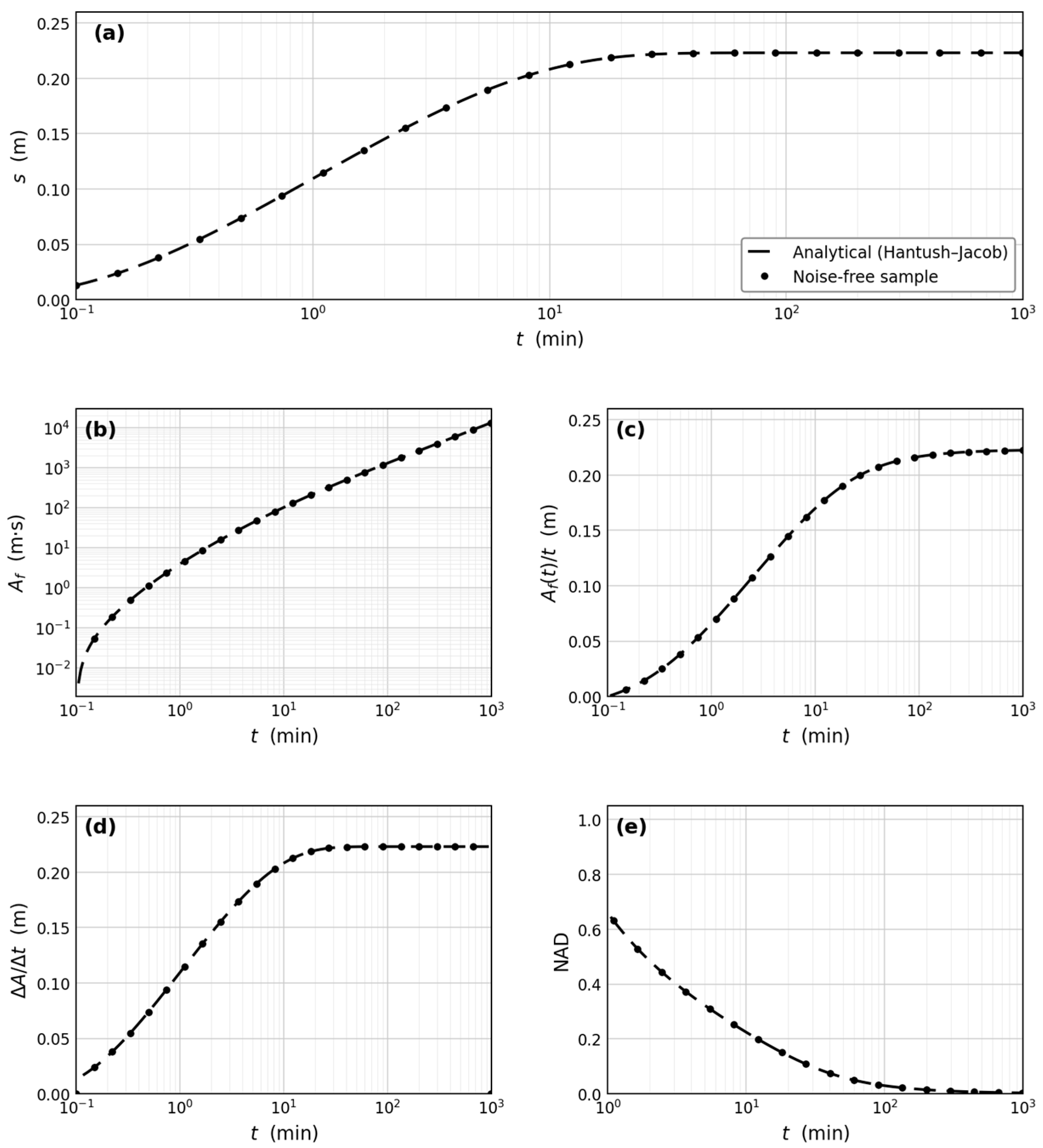
Figure 2 illustrates the four operators applied to a synthetic pumping test generated from the Hantush–Jacob solution with known parameters (T = 1.00 × 10⁻² m2/s, S = 1.00 × 10⁻⁴, B = 250 m, r/B = 0.20, Q = 0.008 m3/s, r = 50 m; s m a x = 0.223 m). All four operators recover the true parameters, demonstrating their complementary sensitivity: A(t) weights the full record; A(t)/t is anchored at the late-time asymptote; ΔAt traces T and B through successive time windows; NAD checks the flow regime independently of parameter fitting. Parameters were estimated by Nelder–Mead simplex minimization; the absement offset A 0 was eliminated analytically, leaving three free parameters.
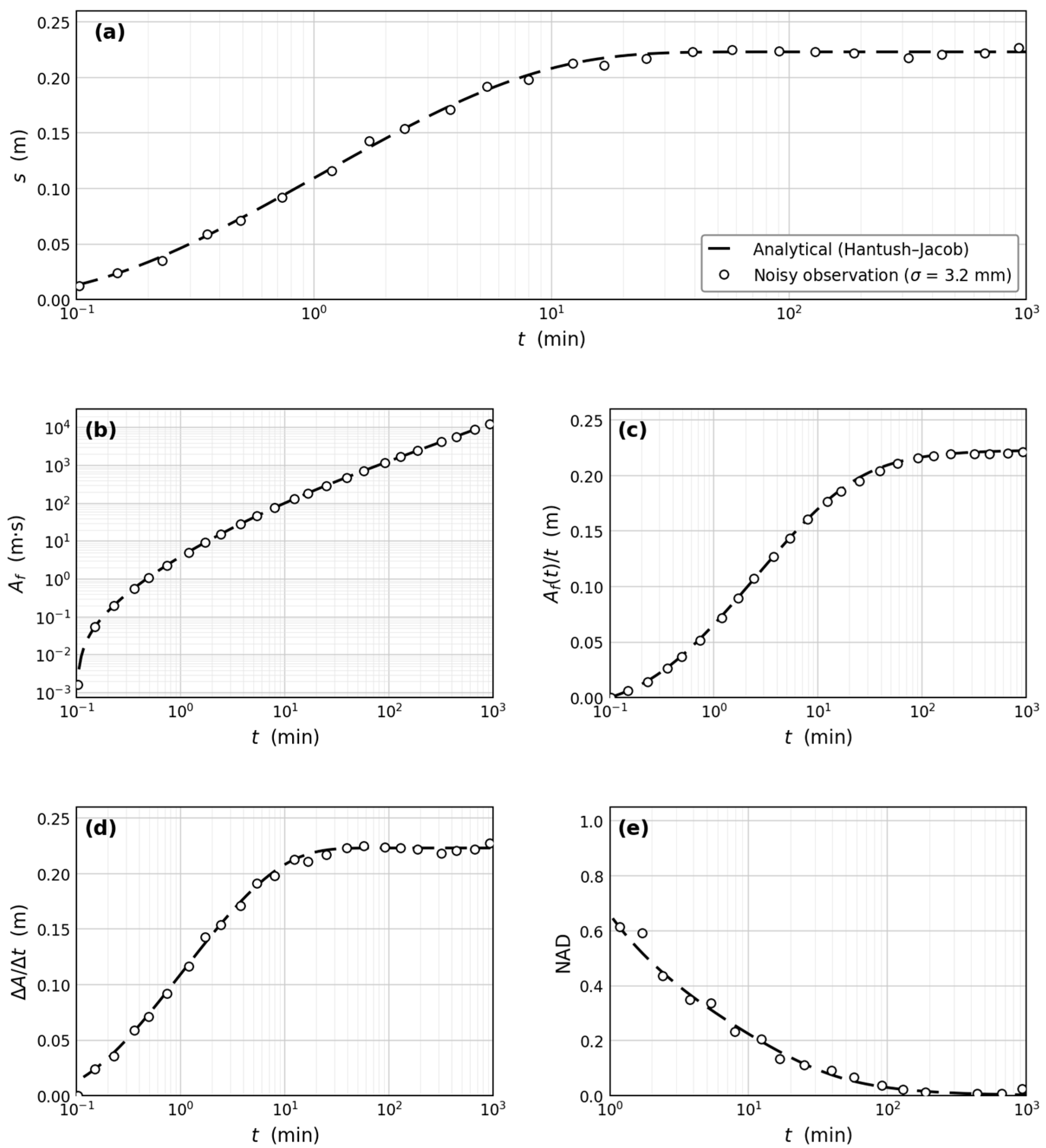
N = 50 Monte Carlo realizations of the Hantush–Jacob solution [5] with composite noise (Gaussian σ = 3 mm, log-time jitter σt = 0.045, quantization Δs = 1 mm) were used to evaluate parameter recovery (Figure 3, Table 3). All four operators recovered T with bias < 0.5%. A(t)/t and ΔA/Δt achieve std(T) of 3.18 × 10⁻⁴ and 3.45 × 10⁻⁴ m2/s, respectively, and std(S) of 4.49 × 10⁻⁶ and 4.95 × 10⁻⁶, respectively, approximately 3–4 times smaller than A(t).

3. Results and Discussions

Three field pumping-test datasets obtained from the literature are analyzed to assess the diagnostic capability of the absement framework. For each case, the four absement operators are applied to the available observation wells, and the results are interpreted jointly to characterize the spatial structure of transmissivity and leakage factor. The results are compared with published conventional analyses to identify what additional information is gained from the absement approach. In every case, only the raw drawdown records are taken from the original publications; the parameter values obtained from the four absement operators, and from the Hantush–Jacob s(t) fit used for comparison, are new analyses carried out in this study and are not the values reported by the original authors.

3.1. Walton [32]—Texas Hill, Salt Flat Drainage Program

The Texas Hill pumping test was conducted in a leaky sandstone aquifer in the Salt Flat drainage district, west Texas, USA. A constant pumping rate of Q = 600 ft3/min (0.2832 m3/s) was maintained for 420 min. Drawdown was measured at three observation wells at radial distances of r = 12.19 m, 24.38 m, and 48.77 m from the pumping well. The test dataset is reproduced in Walton [32] and is widely used as a benchmark for leaky-aquifer analysis methods [1]. T, S, and B were estimated separately using each absement operator for each observation well; Hantush–Jacob s(t) fit is included for comparison. s m a x Values and A(t)/t convergence percentages at the end of the test are shown in the final rows. RMSE computed over all time steps on the Δln t = 0.05 interpolated grid: wells W1, W2, W3, each n = 108.
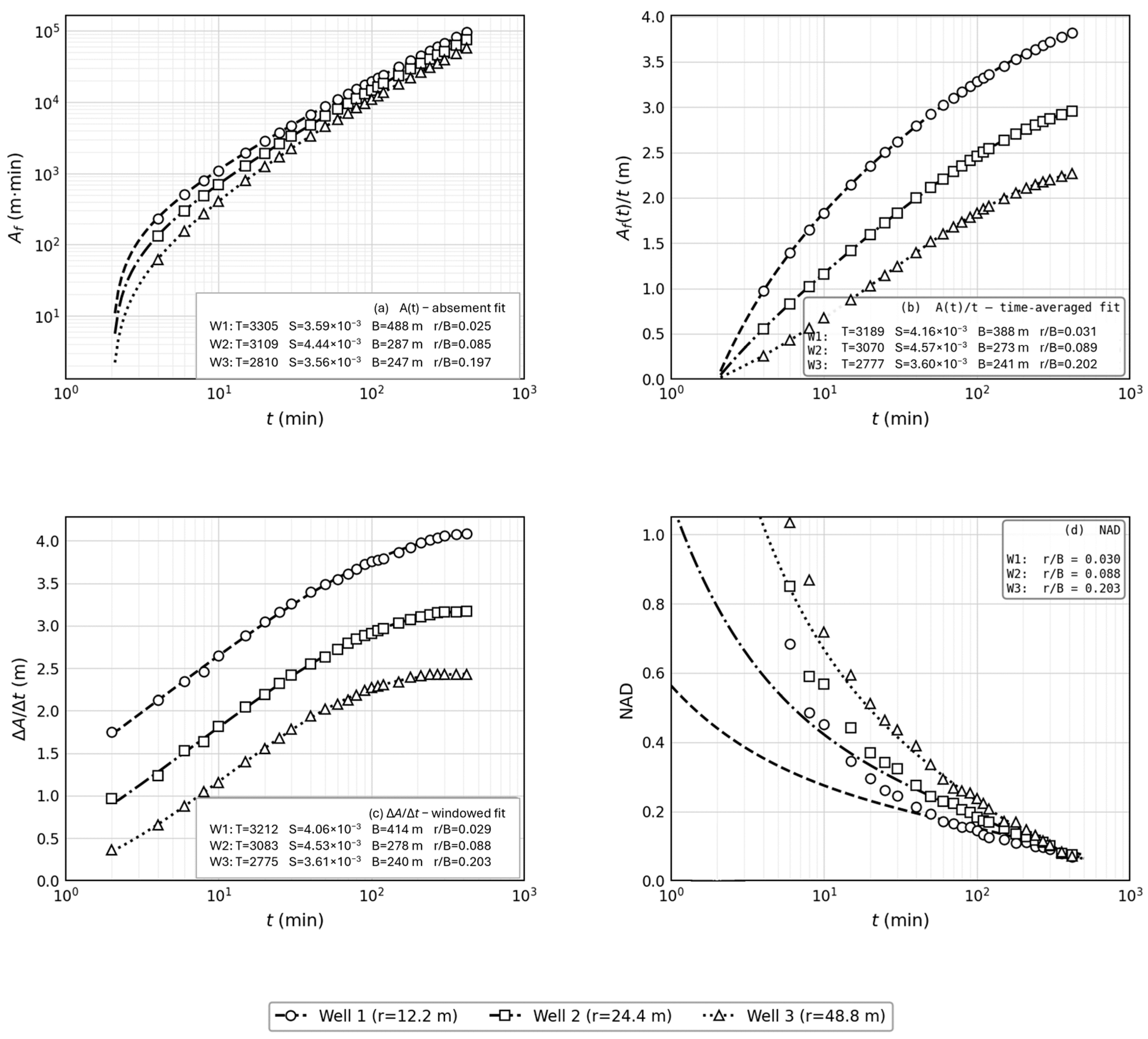
Table 4 presents T, S, and B estimated from each of the four absement operators for each observation well, with each operator fitted separately. All four methods yield mutually consistent estimates within each well: T agrees to within 4%, B within 15%, and S within 12% across operators, consistent with local self-consistency at each location. Figure 4 presents the four operators, A(t), A(t)/t, ΔAt, and NAD, at the three observation wells together with the fitted Hantush–Jacob model curves from which the Table 4 estimates were obtained.
The multi-operator analysis indicates a mild but consistent outward decline in apparent effective transmissivity across the three wells. T decreases from the inner zone (W1, r = 12 m, T ≈ 3200 m2/d) to the middle zone (W2, r = 24 m, T ≈ 3080 m2/d) and the outer zone (W3, r = 49 m, T ≈ 2780 m2/d). The decline is approximately 14% from W1 to W3 and is consistent across all four operators, suggesting it reflects an effective radial-scale feature of the dataset rather than a single-operator fitting artifact. These T values are consistent with Walton’s original conventional type-curve analysis of this dataset. Storativity shows no systematic spatial trend: S ≈ 0.004 at all three wells with mild scatter, indicating that the spatial contrast is primarily in T rather than in storage properties.
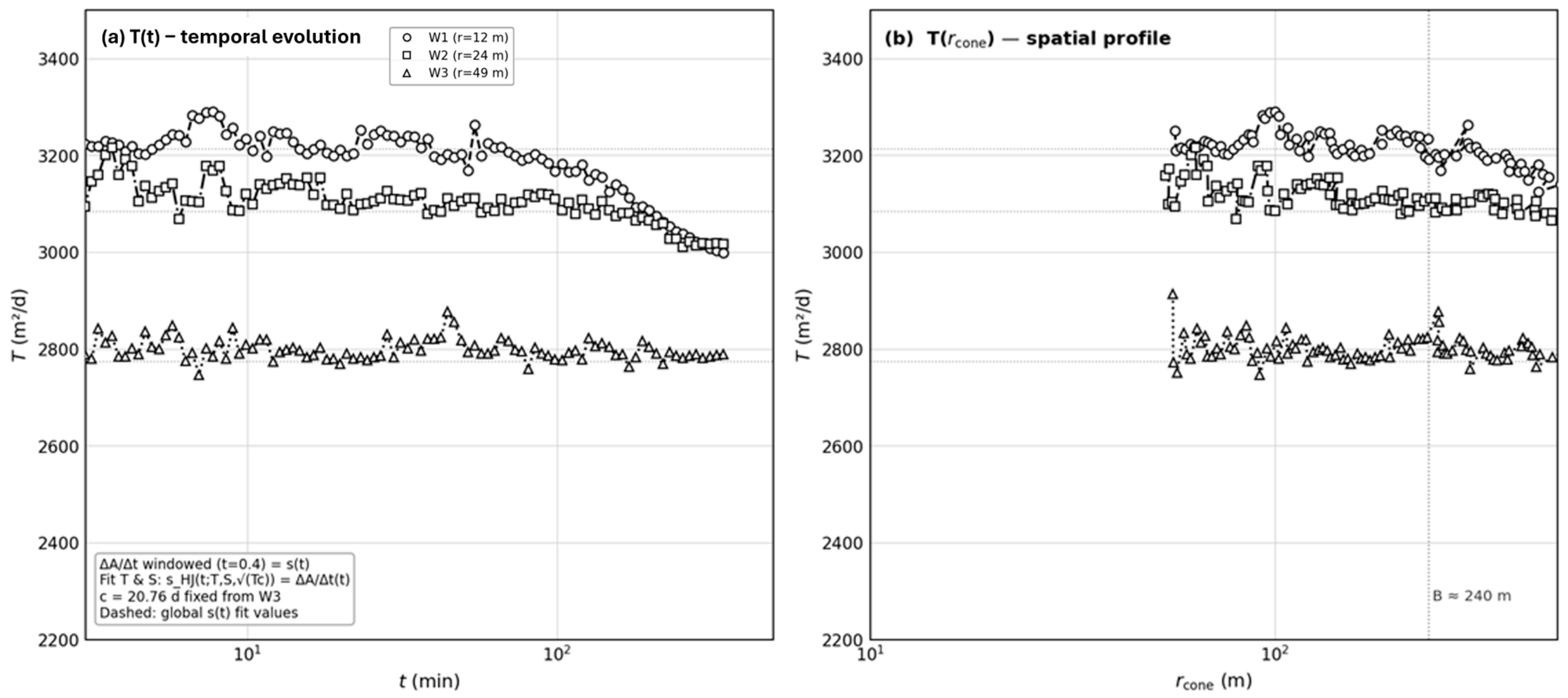
The T(rcone) profiles in Figure 5 were obtained by a windowed fit applied separately to each observation well. The raw drawdown record for each well is interpolated onto a regular Δln t = 0.05 grid. At each window center ti, the ΔAt value is computed from the full-record absement using a Δln t = 0.4 window; since ΔAt equals the smoothed instantaneous drawdown, T is estimated at each window center by matching s_HJ(it; T, S, B = √(T·c)) to the observed ΔAt(it), with S fixed from the global s(t) fit and c = 20.76 d fixed from W3. The aquitard resistance c = B2/T = 20.76 d, recovered from W3 as the best-constrained well (93% A(t)/t convergence, largest r/B = 0.20), is held fixed; B in each window is set to √(Tic), varying naturally as T varies. The NAD profiles at all three wells decay smoothly to zero with no type-curve crossing between wells, supporting spatially uniform B and the use of a common c.
The cone radius at each epoch is computed as rcone = √(2.25·T·t/S) following Copty et al. [19]. All three wells exhibit an early geometric transient in which apparent T is elevated while the cone is being established; beyond rcone ≈ 75–100 m, the profiles stabilize to plateau values of W1 ≈ 3175, W2 ≈ 3086, and W3 ≈ 2794 m2/d. The 14% outward decline in plateau T, supported by non-overlapping bands across all three wells, is consistent with the global per-well fit results in Table 4.
Each profile shows an early geometric transient (elevated apparent T while the cone is being established), followed by a stable plateau; scatter about the plateau reflects sensitivity to windowed-fit noise at individual time steps. In the Walton dataset, the absement analysis recovers parameters consistent with conventional Hantush–Jacob analysis, but also shows that B is spatially stable, that T carries the main spatial contrast, and that steady-state drawdown can be estimated from the same 420 min pumping record. In summary, the Walton test shows a mild outward decrease in transmissivity (≈14% from W1 to W3) with an approximately spatially uniform leakage factor B; here B is plateau-supported at all three wells (A(t)/t convergence 87–93%, most directly at W3).

3.2. De Ridder [33]—Netherlands Leaky Aquifer

The De Ridder [33] pumping test was conducted in a leaky-aquifer in the Netherlands at Q = 31.70 m3/h (8.806 × 10⁻³ m3/s) for 8 h. Drawdown was monitored at four observation wells at r = 30, 60, 90, and 120 m. At W3 (r = 90 m) and W4 (r = 120 m), the drawdown increments in the last time steps are 1–2 mm at the measurement resolution, so the late-time response is close to the leakage-equilibrium plateau. At W1 (r = 30 m) and W2 (r = 60 m) the drawdown is still rising at ≈4 mm/step at the end of the test, so the plateau is not reached at those wells. However, observation of the plateau is not required to determine B from a leaky aquifer test. The absement type-curve family is indexed by r/B in its curve shape, so B can be recovered from any record that captures the curvature transition between the early Theis-confined regime and the late-time plateau. The relevant diagnostic is whether the test duration exceeds the lag-onset time t L , o n s e t B 2 S / ( 10 T ) , at which the curve first departs from the Theis line. All four De Ridder wells satisfy this criterion t L , o n s e t = 2.0–5.4 h, within the 8 h test, so B can be estimated from the full-record global s(t) fit at all four wells via separate three-parameter Nelder–Mead fitting, with wider confidence intervals at W1 and W2 where only the onset of leakage is captured within the 8 h test.
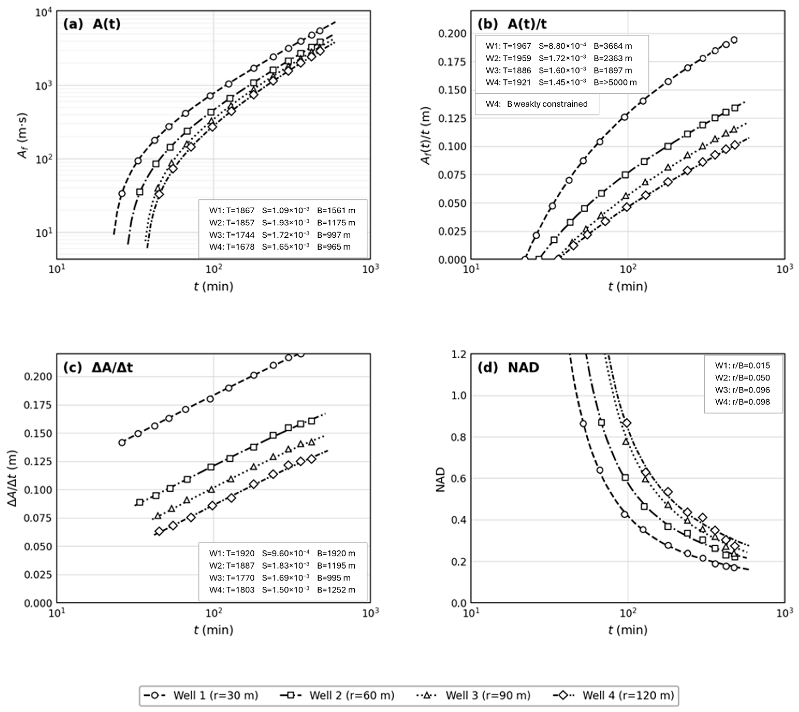
The analysis results are reported in Table 5. Each operator was fitted separately using free three-parameter (T, S, B) Nelder–Mead minimization for each well. RMSE is in drawdown space (m). W1 and W2 did not reach the leakage-equilibrium plateau within the 8 h test; s m a x was not directly observable. Each drawdown record was interpolated onto a Δln t = 0.05 grid, giving n = 63 time steps per well over the 8 h test, from which all RMSE values in Table 5 are computed. Figure 6 presents the four operators at the four observation wells together with the Hantush–Jacob model curves computed from the operator-specific fitted parameters listed in Table 5.
T is approximately homogeneous across all four wells at ≈1750–1950 m2/d, with a modest outward decline of ≈10% from W1 (1928 m2/d) to W3 (1749 m2/d) and no systematic trend beyond that. The reliable spatial signal is in B, which decreases from W1 (2057 m, 95% CI 1668–2790) to W3 (940 m, CI 779–1197), then recovers at W4 (1219 m, CI 911–1999). Storativity is 0.001–0.002 at all wells. RMSE is 1–2 mm in drawdown space across all operators and wells.
Cross-operator agreement is good for s(t), A(t), and ΔAt, with B values within ≈25% at each well. The A(t)/t operator systematically yields larger B across all four wells because the 8 h test does not reach true leakage equilibrium at any well; the cost surface is flat in B when s m a x is not fully observed.
The leakage-onset time t_{L, onset} falls within the 8 h test at all four wells (2.0–5.4 h), providing the curvature needed to determine B from the global fit. Confidence intervals on B are wider at W1 and W2 (≈45% and ≈40%) where only the onset of leakage is captured, and tighter at W3 and W4 (≈23% and ≈45%) where the response approaches the plateau.
T-homogeneity is established by the consistent per-well global fits (all four wells lie within ≈10% of T with no systematic outward trend), and the T(rcone) windowed profile is not computed for this dataset given the short test duration. The NAD decays toward zero at all four wells, supporting the leaky-aquifer flow interpretation throughout, with outer wells decaying faster, consistent with their smaller B. The De Ridder test shows an approximately homogeneous transmissivity (≈1750–1950 m2/d) with a spatially variable leakage factor B that declines outward from W1 to W3 and recovers at W4; B at W3 and W4 is supported by an approach to the plateau, whereas at W1 and W2, where the plateau is not reached, B is a curvature-derived indirect estimate and the A(t)/t value is correspondingly increased.

3.3. Vekol Valley, Arizona [34]—Medium-Grained Sandstone Aquifer

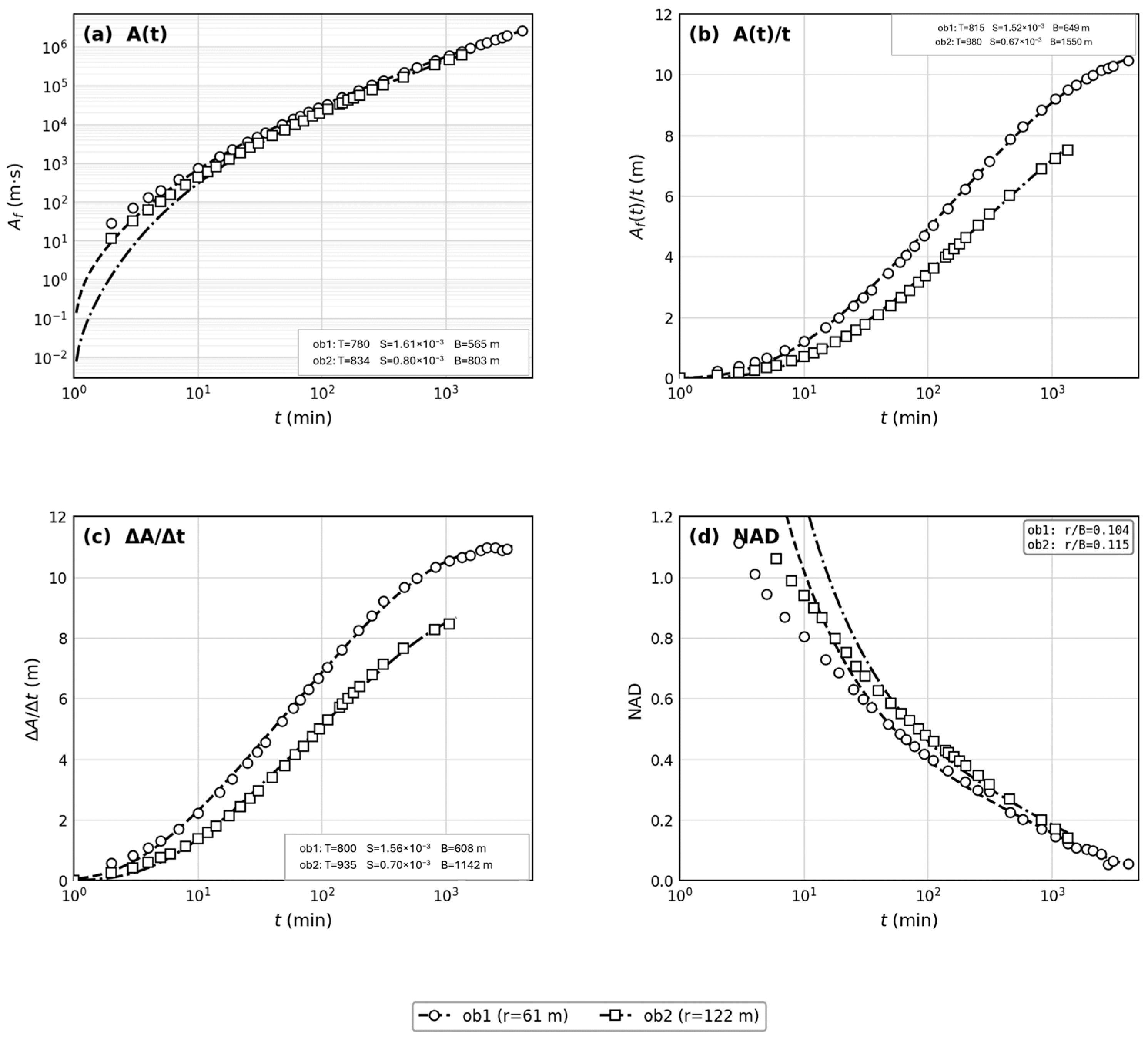
The Vekol Valley pumping test was conducted in a medium-grained sandstone aquifer in Arizona, USA [34]. The pumping well was screened over a 305 m interval. Drawdown was recorded at two observation wells, SV-11ob1 at r = 61 m and SV-11ob2 at r = 122 m; ob1 was monitored for approximately 70 h and ob2 for approximately 22 h. The published pumping rate of Q = 4200 GPM (0.265 m3/s) is adopted throughout this analysis. The drawdown record at ob1 reaches 36.3 ft (11.06 m) at the end of the 70 h test; the fitted s m a x = 11.05 m is consistent with the published Q and the observed drawdown magnitude. Table 6 presents per-operator parameter estimates for both wells. Each operator was fitted separately for each well using free three-parameter Nelder–Mead minimization. RMSE is reported in drawdown space (m). Ob1 reaches 100% of s m a x (11.05 m) at 70 h; Ob2 reaches 93% of s m a x (9.26 m) at 22 h. On the Δln t = 0.05 interpolated grid, this gives n = 168 time steps at ob1 (70 h record) and n = 63 at ob2 (22 h record), over which Table 6 RMSE values are computed. Figure 7 presents the four operators at both observation wells together with the Hantush–Jacob model curves computed from the operator-specific fitted parameters listed in Table 6.
T is approximately homogeneous across both observation wells, with ob1 ≈ 790 m2/d and ob2 ≈ 920 m2/d (approximately 16% cross-well difference), both broadly consistent with the conventional estimate of 929 m2/d. The B estimates show greater variation: ob1 ≈ 590 m (well constrained, 100% convergence); ob2 ≈ 1060–1142 m from s(t) and ΔAt. The A(t)/t operator gives B ≈ 1550 m at ob2, reflecting the flat cost surface when s m a x is not fully observed within the 22 h ob2 record—the same behavior seen in the De Ridder analysis. Cross-operator agreement is good at ob1 (all operators within ≈10% in B); at ob2, the s(t) and ΔAt operators agree well (B ≈ 1060–1142 m) while A(t)/t is inflated.
The s m a x values are: ob1 = 11.05 m (100% convergence at the end of the 70 h test); and ob2 = 9.26 m (93% convergence at the end of the 22 h record). The NAD at both wells decays smoothly toward zero by the end of the test, supporting the Hantush–Jacob leaky-flow interpretation throughout. ob1 follows the r/B ≈ 0.10 type curve, consistent with the fitted B ≈ 590 m and r = 61 m.
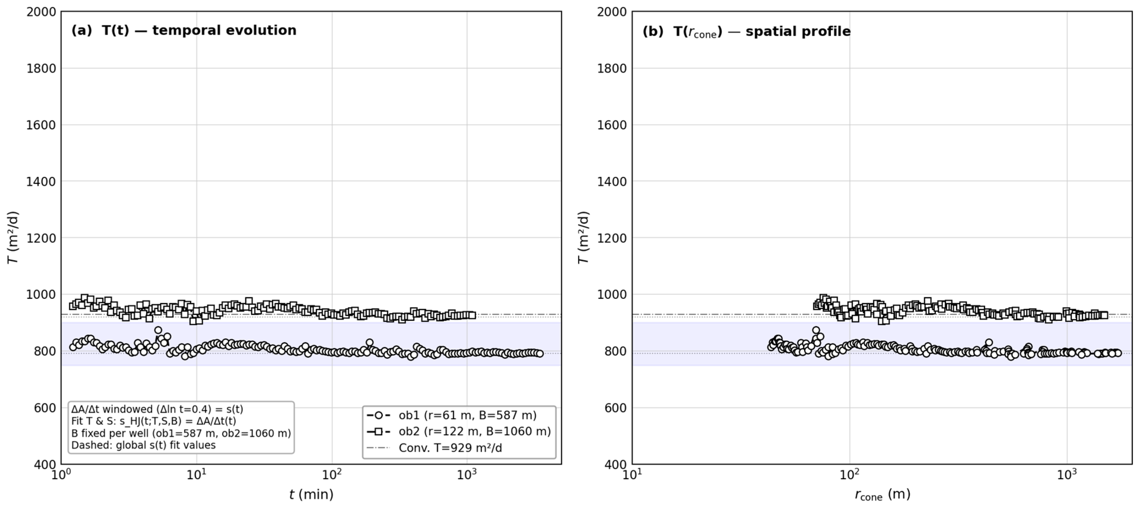
The T(rcone) profiles from the windowed fit (Figure 8) show both wells converging to a common plateau of 750–930 m2/d, consistent with approximately homogeneous T. B is fixed per well from the global s(t) fits (ob1: 587 m, ob2: 1060 m); with B fixed, the windowed ΔAt, which equals the smoothed instantaneous drawdown, constrains T at each window center by matching s_HJ(t; T, S, B) to the observed ΔAt(t), with S fixed from the corresponding global s(t) fit. The convergence of both profiles to the same plateau is consistent with T-homogeneity. The conventional estimate of 929 m2/d may partly reflect TB coupling associated with the larger ob2 B, whereas the windowed fit suggests a lower common effective T.
Using all operators together provides a consistency check unavailable from s(t) alone. All four operators return T within 3% at each well; because the operators weight the record differently, this agreement is stronger evidence of parameter reliability than a single s(t)-based fit. At ob1 (100% convergence), all operators agree on B within 10%. At ob2 (93% convergence), s(t) and ΔAt agree on B within 8%, while A(t)/t gives an inflated value—a diagnostic signal that the cost surface is flat in B and that curvature-sensitive operators are more reliable than the asymptote-dependent one at incomplete convergence. The Vekol Valley test shows an approximately homogeneous transmissivity (≈790–930 m2/d) with a larger leakage factor B at the more distant observation well (ob2); B is plateau-supported at ob1 (100% convergence, observed smax = 11.05 m) but curvature-derived at ob2 (93% convergence), where the A(t)/t value is increased.

4. Implications for Sustainable-Yield Assessment

Sustainable groundwater management requires hydraulic parameters at the spatial and temporal scales relevant to long-term operation [15,30,31]. When test duration and data quality are sufficient, the absement analysis provides three outputs that are useful for sustainable-yield assessment: (i) T(rcone) from ΔAt, anchored to the long-term operating cone; (ii) s m a x from A(t)/t, defining the steady-state drawdown envelope; and (iii) NAD, flagging leakage-regime confirmation and storage-supported early-time yield.
For conservative yield planning in radially expanding tests, the late-cone or outer-well plateau T should generally be preferred over the nearest-well T when the T(rcone) profile shows an outward decline. When T is homogeneous, but B varies spatially, uncertainty in s m a x lies in B through K0(r/B), requiring the spatial B distribution to be mapped across wells.
A practical workflow is therefore as follows: (1) apply NAD to confirm the Hantush–Jacob flow regime and identify any storage-supported early-time yield; (2) read s m a x from the A(t)/t plateau and verify Q consistency; (3) use the ΔAt T(rcone) profile to select the yield-relevant T at the expected operating cone radius; and (4) compare s m a x across wells to identify the binding sustainability constraint. Table 7 summarizes this protocol by aquifer heterogeneity type.
For the De Ridder case, T is homogeneous (≈1750–1950 m2/d), but B decreases outward from 2057 m at W1 to 940 m at W3. The binding sustainability constraint is therefore set by the inner-well leakage factor (B ≈ 940–1219 m at W3–W4), which produces the observed steady-state drawdowns of s m a x = 0.143 m at W3 and 0.129 m at W4. Mapping the spatial B distribution across the four wells, flagged in advance by the NAD type-curve crossing, is essential for a reliable long-term yield estimate in this B-heterogeneous case.
For the Walton case, the yield implication is quantifiable. At Q = 0.2832 m3/s, the steady-state drawdown at W3 (r = 48.8 m, the outermost and most representative well) is s m a x = Q/(2πTK0(r/B) = 2.42 m using the absement-derived outer-well T = 2794 m2/d and B = 240 m—consistent with the observed 2.44 m at 93% convergence. A practitioner using only the near-well T = 3175 m2/d would compute s m a x = 2.13 m at the same location—an underestimate of 0.29 m (14%). Long-term yield planning based on the near-well T therefore overestimates the sustainable pumping rate by approximately 14% relative to the large-scale transmissivity resolved at W3.
For the Vekol case at Q = 0.265 m3/s, the absement-derived parameters (T = 790 m2/d, B = 587 m at ob1) give s m a x = 11.02 m at ob1—in close agreement with the observed 11.05 m. The conventional parameters (T = 929 m2/d, B = 1078 m) give s m a x = 11.73 m—an overestimate of 0.71 m (6%). The conventional analysis underestimates the long-term drawdown because the higher T is compensated by a larger B, shifting the K0(r/B) term. The absement framework resolves this by separately constraining B from the curvature transition and T from the T(rcone) plateau, breaking the TB degeneracy present in a single well s(t) fit.

5. Practical Limitations

The absement operators remain tied to the assumptions of the Hantush–Jacob leaky-aquifer model. The method is most reliable when the pumping rate is stable, the observation-well completion is well documented, early-time wellbore and partial-penetration effects are negligible or identifiable, and the test captures at least the leakage-transition curvature. When the A(t)/t plateau is incomplete, B estimates from A(t)/t should be treated as diagnostic rather than definitive, and greater weight should be placed on curvature-sensitive fits such as s(t), ΔAt, and NAD consistency. Boundary effects, delayed drainage, aquitard storage, and spatially variable leakage can produce similar deviations, so the operator results should be checked against site information and multi-well behavior.

6. Conclusions

This study extends the Absement Method to leaky-aquifer pumping-test analysis. The principal conclusions follow.
  • Governing equations and operators. Time integration of the Hantush–Jacob governing equation yields S·s = T2AC·A, in which T and C occupy structurally distinct terms unavailable in the drawdown domain where they are entangled within W(u, r/B). This structural separation is an exact consequence of the governing physics and provides the analytical reason why the four operators carry complementary information: A(t), the full cumulative integral; A(t)/t, the time-averaged drawdown converging to s m a x ; ΔAt, the windowed incremental rate tracing T(rcone) as the cone expands; and NAD, the normalized absement derivative identifying the flow regime and leakage onset. The A(t)/t asymptote recovers s m a x = Q/(2πTK0(r/B) from transient data without reaching true steady state and independently of S. This is a direct reading when the late-time plateau is actually approached; when convergence is incomplete, s m a x and B are obtained indirectly, as model-based estimates from the curvature of the record, and carry higher uncertainty than a direct reading of the asymptote. The NAD decays to zero at leakage equilibrium—a flow-regime diagnostic absent from derivative-based methods.
  • Performance under measurement noise. Monte Carlo assessment under realistic composite noise shows that A(t)/t and ΔAt recover T, S, and B with negligible bias and standard deviations approximately 3–4 times smaller than those of A(t). Leakage factor B is recovered with standard deviations of approximately 15–16 m for A(t)/t and ΔAt, compared with about 61 m for A(t). The governing equation provides the analytical rationale for why each operator weights a different temporal segment of the drawdown record, an observation that Copty et al. [19] demonstrated through stochastic analysis of discrete interpretation methods in heterogeneous leaky aquifers.
  • Homogeneous and heterogeneous diagnosis. In a homogeneous aquifer, all four operators return consistent {T, S, B} across all observation wells—operator agreement is the indicator. In a heterogeneous aquifer, systematic disagreement between operators becomes part of the interpretation rather than simply a fitting error. The three field cases illustrate distinct heterogeneity signatures: Walton shows an outward decline in T (≈14%, W1 to W3) with spatially uniform B, revealed by non-overlapping T(rcone) bands; De Ridder shows approximately homogeneous T (≈1750–1950 m2/d) with outward-declining B (W1: 2057 m to W3: 940 m), flagged by NAD type-curve crossing before any fitting; and Vekol shows approximately homogeneous T (≈790–930 m2/d) with B increasing outward (ob1: 587 m, ob2: 1060 m), placing it in the B-heterogeneity category alongside De Ridder. Divergent A(t)/t asymptotes and NAD type-curve crossing are visible indicators of B-heterogeneity before formal parameter fitting.
  • Sustainability assessment. When test duration and data quality are sufficient, the framework delivers three sustainability-relevant outputs from a standard pumping-test record without additional instrumentation. The A(t)/t asymptote constrains smax and B most reliably when the leakage-transition curvature and late-time approach to the plateau are sufficiently represented, defining the steady-state drawdown envelope for long-term yield. At incomplete convergence, the asymptote is under-constrained, so greater weight should then be placed on the curvature-sensitive operators (s(t), ΔAt) and on NAD consistency than on the A(t)/t asymptote. The T(rcone) profile identifies transmissivity (T, m2/d) at the operating cone scale; storativity (S) and the leakage factor (B, m) are constrained by the A(t)/t asymptote and the curvature transition. The value differs from the near-well value by up to 14% in Walton, implying a 16% T separation between ob1 and ob2 in Vekol. The NAD confirms whether the leakage regime is fully established, used primarily as a flow-regime and leakage-pattern diagnostic, not as a standalone precise estimator of B. Together, these outputs provide hydraulic constraints for sustainable-yield assessment from routine pumping tests, provided that test duration, data quality, and model assumptions are adequate.

Funding

This research received no external funding.

Data Availability Statement

The original contributions presented in this study are included in the article. Further inquiries can be directed to the corresponding author.

Conflicts of Interest

The author declares no conflicts of interest.

References

  1. Kruseman, G.P.; de Ridder, N.A. Analysis and Evaluation of Pumping Test Data, 2nd ed.; Publication 47; International Institute for Land Reclamation and Improvement (ILRI): Wageningen, The Netherlands, 1992. [Google Scholar]
  2. Woessner, W.W.; Stringer, A.C.; Poeter, E.P. An Introduction to Hydraulic Testing in Hydrogeology: Basic Pumping, Slug, and Packer Methods; The Groundwater Project: Guelph, ON, Canada, 2023. [Google Scholar] [CrossRef]
  3. Theis, C.V. The relation between the lowering of the piezometric surface and the rate and duration of discharge of a well using groundwater storage. Trans. Am. Geophys. Union 1935, 16, 519–524. [Google Scholar] [CrossRef]
  4. Hantush, M.S.; Jacob, C.E. Non-steady radial flow in an infinite leaky aquifer. Trans. Am. Geophys. Union 1955, 36, 95–100. [Google Scholar] [CrossRef]
  5. Hantush, M.S. Analysis of data from pumping tests in leaky aquifers. Trans. Am. Geophys. Union 1956, 37, 702–714. [Google Scholar] [CrossRef]
  6. Hantush, M.S. Modification of the theory of leaky aquifers. J. Geophys. Res. 1960, 65, 3713–3725. [Google Scholar] [CrossRef]
  7. Neuman, S.P.; Witherspoon, P.A. Applicability of current theories of flow in leaky aquifers. Water Resour. Res. 1969, 5, 817–829. [Google Scholar] [CrossRef]
  8. Neuman, S.P.; Witherspoon, P.A. Theory of flow in a confined two-aquifer system. Water Resour. Res. 1969, 5, 803–816. [Google Scholar] [CrossRef]
  9. Batu, V. Aquifer Hydraulics: A Comprehensive Guide to Hydrogeologic Data Analysis; Wiley: New York, NY, USA, 1998. [Google Scholar]
  10. Walton, W.C. Aquifer Test Modelling; CRC Press: Boca Raton, FL, USA, 2007. [Google Scholar]
  11. Dashti, Z.; Nakhaei, M.; Vadiati, M.; Karami, G.H.; Kisi, O. A literature review on pumping test analysis (2000–2022). Environ. Sci. Pollut. Res. 2023, 30, 9184–9206. [Google Scholar] [CrossRef] [PubMed]
  12. Bourdet, D.; Whittle, T.M.; Douglas, A.A.; Pirard, Y.M. A new set of type curves simplifies well test analysis. World Oil 1983, 196, 95–106. [Google Scholar]
  13. Barker, J.A.; Herbert, R. Pumping tests in patchy aquifers. Groundwater 1982, 20, 150–155. [Google Scholar] [CrossRef]
  14. Butler, J.J. Pumping tests in nonuniform aquifers—The radially symmetric case. J. Hydrol. 1988, 101, 15–30. [Google Scholar] [CrossRef]
  15. Butler, J.J.; Liu, W.Z. Pumping tests in nonuniform aquifers: The radially asymmetric case. Water Resour. Res. 1993, 29, 259–269. [Google Scholar] [CrossRef]
  16. Manewell, N.; Doherty, J.; Hayes, P. Translating pumping test data into groundwater model parameters: A workflow to reveal aquifer heterogeneities and implications in regional model parameterization. Front. Water 2024, 5, 1334022. [Google Scholar] [CrossRef]
  17. Copty, N.K.; Sarioglu, M.S.; Findikakis, A.N. Equivalent transmissivity of heterogeneous leaky aquifers for steady state radial flow. Water Resour. Res. 2006, 42, W04416. [Google Scholar] [CrossRef]
  18. Trinchero, P.; Sanchez-Vila, X.; Copty, N.K.; Findikakis, A.N. A new method to interpret pumping tests in leaky aquifers. Groundwater 2008, 46, 133–143. [Google Scholar] [CrossRef] [PubMed]
  19. Copty, N.K.; Trinchero, P.; Sanchez-Vila, X.; Sarioglu, M.S.; Findikakis, A.N. Influence of heterogeneity on the interpretation of pumping test data in leaky aquifers. Water Resour. Res. 2008, 44, W11419. [Google Scholar] [CrossRef]
  20. Zhuang, C.; Li, Y.; Zhou, Z.; Illman, W.A.; Dou, Z.; Yang, Y.; Wang, J. Effects of exponentially decaying aquitard hydraulic conductivity on well hydraulics and fractions of groundwater withdrawal in a leaky aquifer system. J. Hydrol. 2022, 607, 127439. [Google Scholar] [CrossRef]
  21. Zhuang, C.; Zhan, H.B.; Xu, X.D.; Wang, J.G.; Zhou, Z.F.; Dou, Z. Effects of aquitard windows on groundwater fluctuations within a coastal leaky aquifer system: An analytical and experimental study. Adv. Water Resour. 2023, 177, 104473. [Google Scholar] [CrossRef]
  22. Zhuang, C.; Lü, C.; Yan, L.; Li, Y.; Zhou, Z.; Wang, J.; Dou, Z.; Illman, W.A. Pumping-induced well hydraulics and groundwater budget in a leaky aquifer system with vertical heterogeneity in aquitard hydraulic properties. Acta Geol. Sin.—Engl. Ed. 2024, 98, 477–490. [Google Scholar] [CrossRef]
  23. Meng, X.; Zhang, W.; Wang, Q.; Yin, M.; Liu, D. Modeling of low-velocity non-Darcian flow with nonlinear consolidation in a leaky aquifer system induced by a fully penetrating confined well. Water Resour. Res. 2025, 61, e2024WR038370. [Google Scholar] [CrossRef]
  24. De Smedt, F. Determination of aquitard storage from pumping tests in leaky aquifers. Water 2023, 15, 3735. [Google Scholar] [CrossRef]
  25. van Leer, M.D.; Zaadnoordijk, W.J.; Zech, A.; Griffioen, J.; Bierkens, M.F.P. Mapping the spatial sensitivity of aquitard hydraulic parameters on pumping test drawdowns. Groundwater 2025, 64, 41–48. [Google Scholar] [CrossRef] [PubMed]
  26. Li, W.; Nowak, W.; Cirpka, O.A. Geostatistical inverse modeling of transient pumping tests using temporal moments of drawdown. Water Resour. Res. 2005, 41, W08403. [Google Scholar] [CrossRef]
  27. Zhu, J.; Yeh, T.C.J. Analysis of hydraulic tomography using temporal moments of drawdown recovery data. Water Resour. Res. 2006, 42, W02403. [Google Scholar] [CrossRef]
  28. Blasingame, T.A.; Johnston, J.L.; Lee, W.J. Type-curve analysis using the pressure integral method. In Proceedings of the SPE California Regional Meeting, Bakersfield, CA, USA, 5–7 April 1989. SPE 18799. [Google Scholar] [CrossRef]
  29. Palacio, J.C.; Blasingame, T.A. Decline-curve analysis using type curves—Analysis of gas well production data. In Proceedings of the SPE Rocky Mountain Regional/Low Permeability Reservoirs Symposium, Denver, CO, USA, 26–28 April 1993; SPE 25909. Available online: https://blasingame.engr.tamu.edu/0_TAB_Public/TAB_Publications/SPE_025909_(Palacio)_Blasingame_Gas_Well_Dec_TC_Anl.pdf (accessed on 28 June 2026).
  30. Avcı, C.B.; Sahin, U.; Ciftci, E. Aquifer parameter estimation using an incremental area method. Hydrol. Process. 2011, 25, 2584–2596. [Google Scholar] [CrossRef]
  31. Avcı, C.B. Cumulative drawdown as a primary state variable: The Absement Method for confined aquifer pumping-test analysis. Water 2026, 18, 1143. [Google Scholar] [CrossRef]
  32. Walton, W.C. Selected Analytical Methods for Well and Aquifer Evaluation; Illinois State Water Survey Bulletin 49; Illinois State Water Survey: Urbana, IL, USA, 1962. [Google Scholar]
  33. De Ridder, N.A. Analysis of the Aquifer Test at Dalfsen in the Eastern IJssel-Vecht Area; TNO Rapport; Dienst Grondwaterverkenning; TNO: Delft, The Netherlands, 1961. [Google Scholar]
  34. Marie, J.R.; Hollett, K.J. Determination of Hydraulic Characteristics and Yield of Aquifers Underlying Vekol Valley, Arizona, Using Several Classical and Current Methods; U.S. Geological Survey Water-Supply Paper 2453; U.S. Geological Survey: Reston, VA, USA, 1996; 63p.
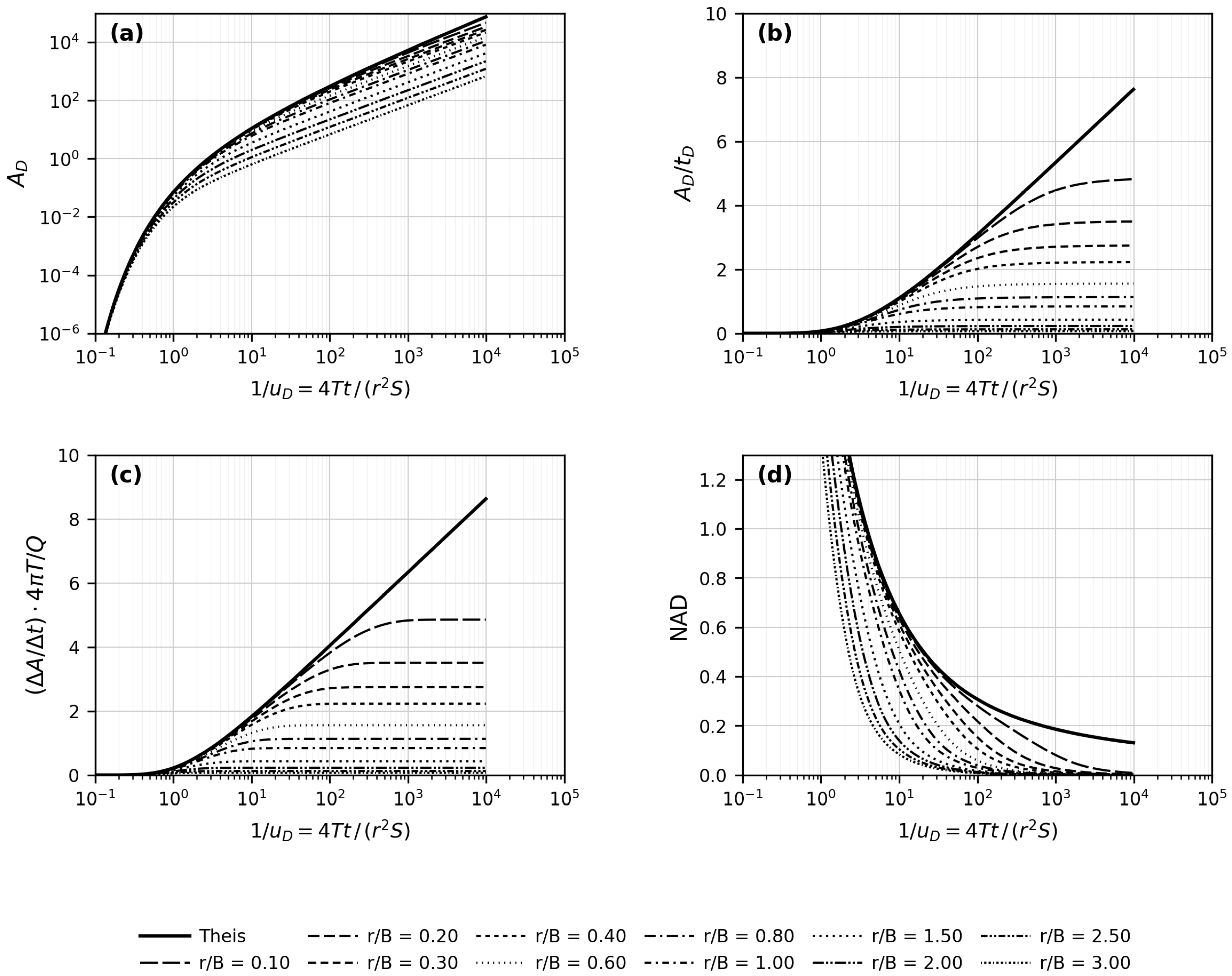
Figure 1. Hantush–Jacob leaky-aquifer dimensionless absement type curves. Family parameterized by r/B, from the Theis confined-aquifer limit (r/B = 0-Theis solid black line) to r/B = 3.0, where 1/uD = 4Tt/(r2S) is the dimensionless time parameter. (a) Dimensionless absement AD (the normalized form of the physical operator A(t)) vs. 1/uD; (b) time-averaged absement A D / t D approaching the leakage asymptote 2 K 0 ( r / B ) ; (c) windowed increment ΔAt at Δ l n ( t )   =   0.2 ; (d) normalized absement derivative (NAD), decaying to zero at full leakage equilibrium.
Water 18 01638 g001
Figure 2. Noise-free synthetic Hantush–Jacob baseline. (a) Drawdown overlaid on the analytical curve; (b) absement A(t) on log–log scale; (c) time-averaged absement A(t)/t; (d) windowed ΔAt; (e) NAD.
Water 18 01638 g002
Figure 3. Synthetic Hantush–Jacob example: noisy drawdown record and recovered absement operators. (a) Noisy drawdown overlaid on the analytical curve; (b) absement A(t) on log–log scale; (c) time-averaged absement A(t)/t; (d) windowed ΔAt; (e) NAD.
Water 18 01638 g003
Figure 4. Walton [32] Texas Hill—all four absement operators at all three wells (Q = 0.2832 m3/s). Open markers: raw field observations. Dashed lines: Hantush–Jacob model curves using operator-specific fitted parameters per well.
Water 18 01638 g004
Figure 5. Walton [32] Texas Hill—T(t) and T(rcone) profiles. (a) Apparent T as a function of time; (b) apparent T as a function of cone radius. Windowed joint fit: Δln t = 0.4; T free; S fixed from s(t) fit; B = √(Tc), c = 20.76 d fixed from W3. Faint dashed lines: global per-well s(t) fit values (Table 4).
Water 18 01638 g005
Figure 6. De Ridder [33] Netherlands—all four operators, four wells (Q = 8.806 × 10⁻³ m3/s) each fitted by free three-parameter (T, S, B) Nelder–Mead minimization per operator. Open markers: raw field observations. Dashed lines: Hantush–Jacob model curves using operator-specific fitted parameters per well.
Water 18 01638 g006
Figure 7. Vekol Valley [34] Arizona—all four absement operators at both observation wells (Q = 0.265 m3/s, 4200 GPM). Open markers: raw field observations. Dashed lines: Hantush–Jacob model curves using operator-specific fitted parameters per well.
Water 18 01638 g007
Figure 8. Vekol Valley [34] Arizona—T(rcone) from windowed fit (Δln t = 0.4; T free; S fixed from s(t) fit; B fixed per well: ob1 B = 587 m, ob2 B = 1060 m). At each window center, T is obtained by matching s_HJ(t; T, S, B) to the observed ΔAt(t), with S fixed from the corresponding global s(t) fit. Open circles (ob1, r = 61 m) and open squares (ob2, r = 122 m): windowed T estimates. Dotted horizontal lines: global per-well s(t)-fit T values (Table 6). Dash–dot horizontal line: conventional estimate of 929 m2/d. Light-purple shaded band: common plateau range of the windowed-fit T estimates encompassing both wells.
Water 18 01638 g008
Table 1. Homogeneous aquifer: parameter identifiability from the four absement operators.
OperatorTSsmaxB
A(t)Reliable; early-time slope gives T (though A(t)/t and ΔAt reach lower σT)Reliable; sets curve position, well resolved from full-record fitNot direct; derived from T and B after fittingEstimable but less precise than A(t)/t; ~5× larger uncertainty (Table 3)
A(t)/tReliable; from global curve shape, S separates analyticallyWeakly constrained; drops out of the asymptoteDirect from late-time plateau; only operator giving smax without first fitting T, B; independent of SMost precise; from smax and T via K0(r/B)
ΔAtSpatial T(rcone) profile per windowNot direct; enters via rcone axis onlyNot available; use A(t)/tIndirect; late-time ΔAtsmax gives a second B near the plateau, else qualitative (plateau-onset timing only)
NADIndirect; shifts type curve in time, not separable from B without fittingIndirect; shifts type curve like T, not separable from NAD aloneNot estimated; flow-regime diagnostic onlyDiagnostic constraint on r/B pattern; not a standalone B estimator
Table 2. Heterogeneous or non-ideal aquifer: what each operator returns and its spatial meaning.
OperatorTSsmaxB
A(t)Time-weighted average T over the cone path; near-well dominates (early data weighted most)Weighted average S over the cone path; not a local valueIndirect; depends on cone-path averages of T, B; may differ from true smaxCone-path average B; blends near-well and far-field leakage
A(t)/tEffective T over the leakage-bounded cone at convergenceNot recovered; drops out of the asymptoteMost stable smax; anchored at steady state, S-independent even under heterogeneityEffective B at the cone boundary; per-well values map the spatial B pattern
ΔAtApparent T(rcone) per window; systematic slope flags radial T variation or model mismatchNot resolved; S shifts the rcone axis, not separableNot available; use A(t)/tQualitative; differing leakage-transition timing between wells indicates B(r) variation
NADIndirect; systematic NAD shift between wells flags T variationIndirect model check; early-time NAD above the Hantush–Jacob curve may indicate aquitard storage SNot estimated; flow-regime and model-check diagnostic onlySpatial B signal; migration across r/B type curves flags B(r) variation
Table 3. Monte Carlo parameter recovery (N = 50 realizations; 200 log-spaced time points per realization; T = 0.01 m2/s, S = 1 × 10⁻⁴, B = 250 m, r = 50 m, Q = 0.008 m3/s).
Analysis MethodT Mean (m2/s)T Std (m2/s)S MeanS StdB Mean (m)B Std (m)RMS Mean
Absement A(t)0.0100331.11 × 10−31.03 × 10−41.05 × 10−5257.261.23.23 × 10−3 m
Absement A(t)/t0.0100113.18 × 10−41.01 × 10−44.49 × 10−6251.015.23.03 × 10−3 m
Discr. ΔAtln t = 0.2)0.0099873.45 × 10−49.98 × 10−54.95 × 10−6250.016.43.03 × 10−3 m
NAD0.0100324.53 × 10−49.08 × 10−52.08 × 10−5291.060.42.01 × 10−2 m
True values0.0100001.00 × 10−4250.0
Notes: RMS for A(t) is in absement space (m·s); for A(t)/t and ΔAt it is in meters. B is the leakage factor (m); r/B = 50/250 = 0.20.
Table 4. Parameter estimates for the Walton [32] Texas Hill pumping test (Q = 0.2832 m3/s, 420 min).
MethodW1 r = 12.19 mW2 r = 24.38 mW3 r = 48.77 mRMSE (m) W1RMSE (m) W2RMSE (m)
W3
T [m2/d]SB [m]T [m2/d]SB [m]T [m2/d]SB [m]
A(t)33050.0035948831090.0044428728100.003562470.15800.03840.0142
A(t)/t31890.0041638830700.0045727327770.003602410.13000.03260.0139
ΔAt32120.0040641430830.0045327827750.003612400.14300.03500.0134
Hantush–Jacob s(t)32120.0040641330840.0045327827740.003612400.14200.03440.0135
s m a x [m]4.413.232.44
Conv. [%]879293
Table 5. Parameter estimates for the De Ridder [33] Netherlands pumping test (Q = 8.806 × 10⁻³ m3/s, 8 h).
MethodW1 (r = 30 m)W2 (r = 60 m)
T [m2/d]SB [m]RMSET [m2/d]SB [m]RMSE
s(t)19280.0009520570.000918830.0018511940.0012
A(t)18670.0010915610.001118570.0019311750.0013
A(t)/t19670.0008836640.001119590.0017223630.0015
ΔAt19200.0009619200.000918870.0018311950.0012
smax [m]
MethodW3 (r = 90 m)W4 (r = 120 m)
T [m2/d]SB [m]RMSET [m2/d]SB [m]RMSE
s(t)17490.001699400.001317920.0015012190.0016
A(t)17440.001729970.001516780.001659650.0018
A(t)/t18860.0016018970.002019210.0014524000.0020
ΔAt17700.001699950.001418030.0015012520.0016
smax [m] a0.143 (obs.)0.129 (obs.)
Notes: a W1 and W2 did not reach the leakage-equilibrium plateau within the 8-h test; smax was not directly observable.
Table 6. Parameter estimates for the Vekol Valley pumping test (Q = 0.265 m3/s, 4200 GPM).
Methodob1 (r = 61 m)ob2 (r = 122 m)
T [m2/d]SB [m]RMSET [m2/d]SB [m]RMSE
s(t)7900.001605870.1259200.0007110600.097
A(t)7800.001615650.1288340.000808030.133
A(t)/t8150.001526490.1359800.0006715500.130
ΔAt8000.001566080.1279350.0007011420.100
Table 7. Recommended absement operator protocol for sustainable-yield assessment by aquifer heterogeneity type.
Heterogeneity TypeField CaseKey Diagnostic SignalYield Assessment Action
Mild outward T decline; S approximately constantWaltonNAD decays to zero at all three wells; T(rcone) declines 14% from W1 to W3Use outer-well T (≈2794 m2/d) for large-scale yield; near-well T (≈3175 m2/d) for near-field. Min s m a x = 2.44 m (W3) defines the sustainability envelope
Approximately homogeneous T; spatially variable BDe RidderNAD type-curve crossing between wells flags B-heterogeneity before fittingUse T ≈ 1750–1950 m2/d; account for outward B variation when estimating leakage-supported long-term response (T-homogeneous within ≈10% across all four wells). B varies outward: W1 B = 2057 m to W3 B = 940 m, flagged by NAD type-curve crossing before any fitting. smax at W3 (0.143 m) and W4 (0.129 m) define the leakage-controlled sustainable-yield ceiling.
Approximately homogeneous T (≈790–930 m2/d); B increases outwardVekol ValleyNAD confirms leaky regime; ob1 reaches full convergence, while ob2 reaches 93% convergence. At ob2, B is constrained primarily by s(t) and ΔAt curvature rather than by the A(t)/t asymptoteUse T ≈ 870 m2/d; s m a x from ob1 well established (11.05 m); ob2 s m a x (9.26 m) confirmed at 93% convergence
Disclaimer/Publisher’s Note: The statements, opinions and data contained in all publications are solely those of the individual author(s) and contributor(s) and not of MDPI and/or the editor(s). MDPI and/or the editor(s) disclaim responsibility for any injury to people or property resulting from any ideas, methods, instructions or products referred to in the content.