Seasonal Dynamics of Inter-Device Discrepancies and Their Key Influencing Factors in Monitoring Water Surface Evaporation

Abstract

Accurate comparison of water-surface evaporation observations from different devices is essential for integrating long-term hydrological records. This study analyzed two years of synchronous daily observations from five co-located evaporation devices in Duyun, Guizhou, China: D20, E601, and three evaporation ponds with surface areas of 1, 5, and 20 m² (P1, P5, and P20). Evaporation differences, conversion coefficients, correlations, and statistical variability were evaluated at annual, seasonal, monthly, and daily scales. The main findings were as follows: (1) among the three similarly constructed ponds, annual evaporation decreased from 946 mm for P1 to 896 mm for P5 and 874 mm for P20, whereas the annual totals measured by D20 and E601 were 842 and 861 mm, respectively; (2) the relationship among the three ponds varied within the year, reversing in July and August and becoming non-monotonic in May and June; (3) pairwise correlations were generally strongest in summer and weakest in winter, indicating pronounced seasonal variation in inter-device relationships; and (4) because D20 was installed above ground whereas E601 and the three ponds were buried, differences among all five devices reflected combined scale- and design-related effects, while comparisons among the three ponds primarily represented surface-area-related effects. These findings provide a site-specific basis for harmonizing evaporation records and improving their application in hydrological and water-balance studies.

1. Introduction

Evaporation from open water surfaces is a fundamental process in the exchange of water and energy between the Earth’s surface and the atmosphere and plays an important role in the terrestrial hydrological cycle and climate system [1,2]. Accurate measurement of water-surface evaporation is essential for water-resource management, agricultural production, and ecosystem sustainability [3,4,5] and provides important information for hydrological modeling and climate-change research [6,7,8,9].

Several approaches are currently used to observe or estimate evaporation. Standard evaporation pans directly measure water loss from standardized containers and remain among the earliest and most widely used instruments in meteorological and hydrological observation networks [10,11]. Field-based methods, including eddy covariance and soil-moisture monitoring techniques such as time-domain reflectometry, estimate surface water losses from energy fluxes or changes in soil-water storage [12,13]. Remote-sensing approaches use satellite- or unmanned-aerial-vehicle-based observations, together with energy-balance models or vegetation indices, to estimate evaporation or evapotranspiration at regional scales [14,15,16,17]. Despite rapid advances in these techniques, standard evaporation pans remain indispensable because of their operational simplicity, relatively low cost, ease of maintenance, and ability to provide continuous long-term records [18,19].

A persistent challenge in pan evaporation observations is the diversity of instruments adopted by different countries and regions. In the United States, the Class A evaporation pan, with a diameter of 1.21 m and a depth of 0.25 m, is widely used in meteorological and agricultural observations [20]. In Australia, the Sunken Pan is embedded in the ground to reduce excessive sidewall heating and better approximate the thermal conditions of natural water bodies, particularly in arid environments [21]. In parts of Europe, the smaller Symons pan, with a diameter of approximately 0.2 m, facilitates spatially distributed observations but is relatively sensitive to variations in wind and radiation [22]. In China, two standard instruments—the D20 and E601 pans—have been extensively operated by meteorological and hydrological agencies [23,24]. The D20 pan has a diameter of 20 cm and is installed 70 cm above the ground, whereas the E601 pan has a diameter of approximately 1.2 m and is buried below ground. Owing to its larger water volume, greater thermal storage capacity, and buried installation, the E601 pan is less sensitive to short-term meteorological fluctuations and is generally considered more representative of natural water-surface evaporation [25]. The coexistence of devices with markedly different dimensions and installation configurations has therefore prompted extensive research on their observational differences and conversion relationships [26,27,28,29].

Previous studies have mainly examined conversion coefficients, meteorological controls, and practical applications involving one or two types of evaporation devices. Sabziparvar et al. [18] used Class A pan observations to derive coefficients applicable under different climatic conditions. Shen et al. [24] developed a PenPan-D20-based framework to attribute changes in pan evaporation to multiple meteorological drivers. Qian et al. [26] applied machine-learning models to predict and convert pan evaporation records from multiple stations in southern China. Li et al. [27] investigated the transition from D20 to E601 pans in the Yangtze River Basin and reported conversion coefficients ranging from 0.55 to 0.80. Li et al. [28] identified seasonal variations in the conversion coefficient between D20 and E601B pans and found net radiation to be an important influencing factor. These studies have improved the continuity, correction, and application of evaporation records obtained using different instruments.

Nevertheless, important gaps remain. Most previous studies have compared only one or two devices, particularly D20 and E601, and therefore cannot determine how evaporation varies across a broader range of surface areas. In addition, many conversion relationships have been derived from data collected at different locations or during non-overlapping periods, making it difficult to separate device effects from spatial and temporal variations in meteorological conditions. Differences among devices also cannot be attributed to surface area alone because pan size commonly varies together with water depth, geometry, installation height, thermal storage, and exposure to the surrounding ground and atmosphere. The observed discrepancies therefore reflect combined scale- and design-related effects [29,30]. Moreover, annual or seasonal conversion coefficients may conceal monthly changes caused by seasonal variations in radiation, air temperature, humidity, and wind speed [31]. These limitations highlight the need for synchronous, co-located observations involving multiple devices with a wide range of sizes and structural configurations.

To address these gaps, we established a co-located monitoring experiment at a standard meteorological station in the karst region of Guizhou, China. This region is characterized by thin soils, high permeability, and rapid subsurface drainage, where surface evaporation plays a particularly critical role in the regional water balance and local water resource management. Five evaporation devices were operated simultaneously over a two-year period: two nationally used standard pans, D20 and E601, and three evaporation ponds with depths of 3 m and surface areas of 1, 5, and 20 m², hereafter referred to as P1, P5, and P20, respectively. Because the three ponds share the same water depth, material, and installation configuration, their comparison primarily reflects differences associated with water-surface area. In contrast, comparisons involving D20 and E601 represent the combined effects of size, geometry, water depth, and installation design, corresponding to the practical challenge of integrating observations from different monitoring systems. Using these synchronous observations, this study quantified evaporation differences among the five devices at daily, monthly, seasonal, and annual scales and evaluated their conversion coefficients, pairwise correlations, and statistical variability. The originality of this study lies in the co-located and synchronous comparison of five devices spanning a wide range of water-surface areas, the distinction between surface-area-related differences among the three similarly constructed ponds and the combined scale- and design-related effects involving the standard pans, and the identification of intra-annual variations that may be obscured by annual aggregation. The findings provide a site-specific basis for harmonizing evaporation records and improving their application in hydrological modeling, reservoir water-balance assessment, and water-resource management.

2. Data and Methods

2.1. Evaporation Facilities Setting and Regional Overview

2.1.1. Evaporation Monitoring Equipment Layout

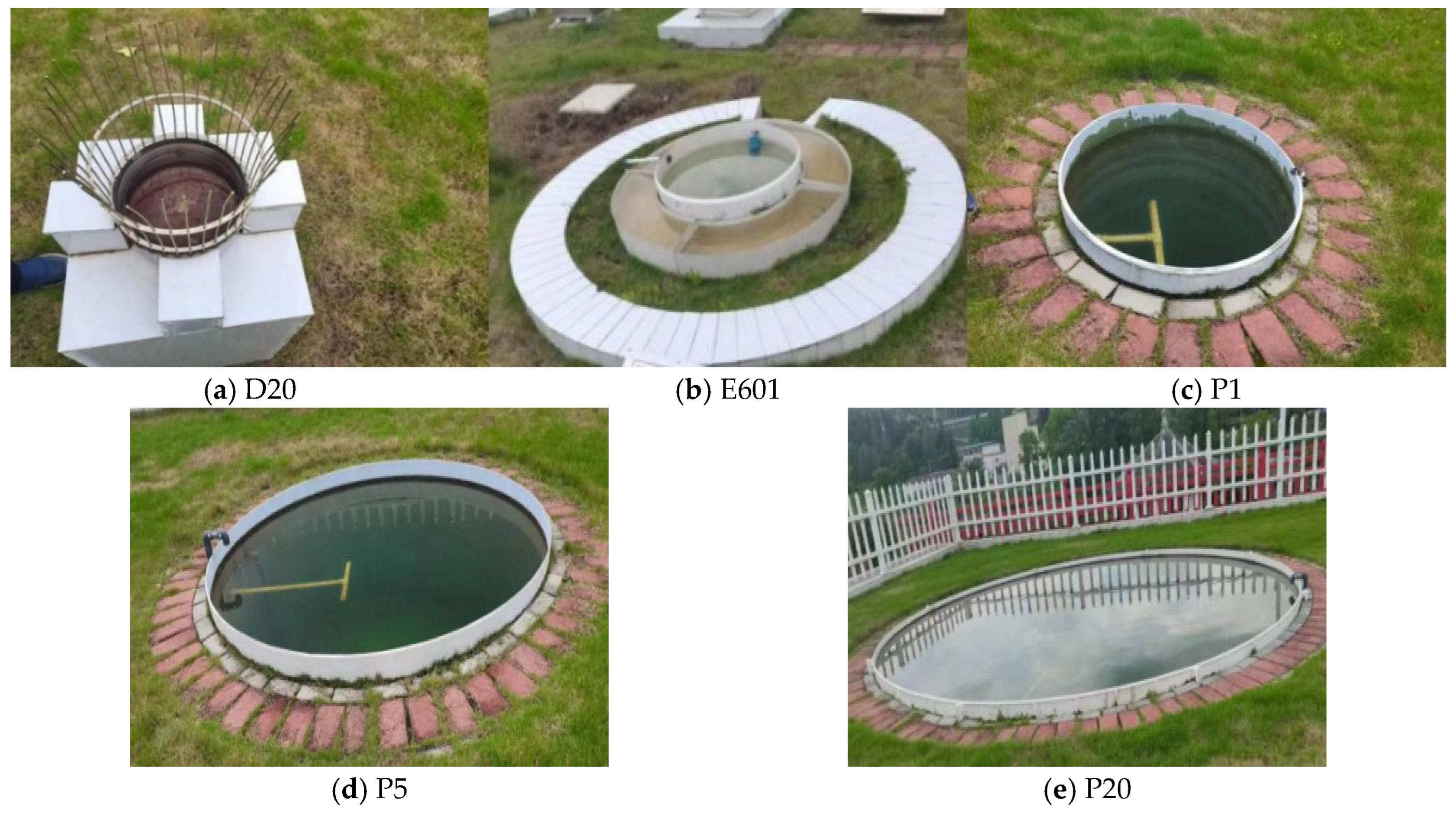
This study selects the E601 evaporation pan as the reference instrument, along with four other evaporation monitoring devices: a small pan D20 and three other evaporation pond with water depth of 3 m and surface area of 1 m², 5 m², and 20 m² (denoted as P1, P5 and P20) to monitor daily evaporation data. The specifications of these devices are provided in

Table 1. Specifications of different evaporation equipment.

Monitor Devices	Diameter (m)	Area (m2)	Installation Method	Water Depth (cm)	Material
E601	0.618	0.3	Embedding method	60	Plastic
D20	0.2	0.0314	Suspension type	20	Plastic
P1	1.128	1	Embedding method	300	Plastic
P5	2.523	5	Embedding method	300	Plastic
P20	5.046	20	Embedding method	300	Plastic

. The evaporation pans are deployed at a standard meteorological monitoring site, with their essential characteristics and installation details shown in Figure 1. The E601, and the three evaporation ponds are installed below ground level, surrounded by grass cover, and the water-holding material is plastic. The installation of the D20 pan at a height of 70 cm above ground complies with the national standard Ground Meteorological Observation Specification [32]. In contrast, the E601, P1, P5, and P20 pans are installed using a buried method to better simulate the conditions of natural water bodies [33]. The differences in installation methods, depths, etc. belong to the “design effect”, which are confounding factors that cannot be completely excluded in this study, but their influences will be fully considered. No specific permits were required for this study, as the field site is a designated meteorological observation station operated by Bureau of Hydrology and Water Resources of Qiannan Autonomous Prefecture of Guizhou Province, and all data collection was conducted under their institutional research framework.

2.1.2. Overview of Test Area

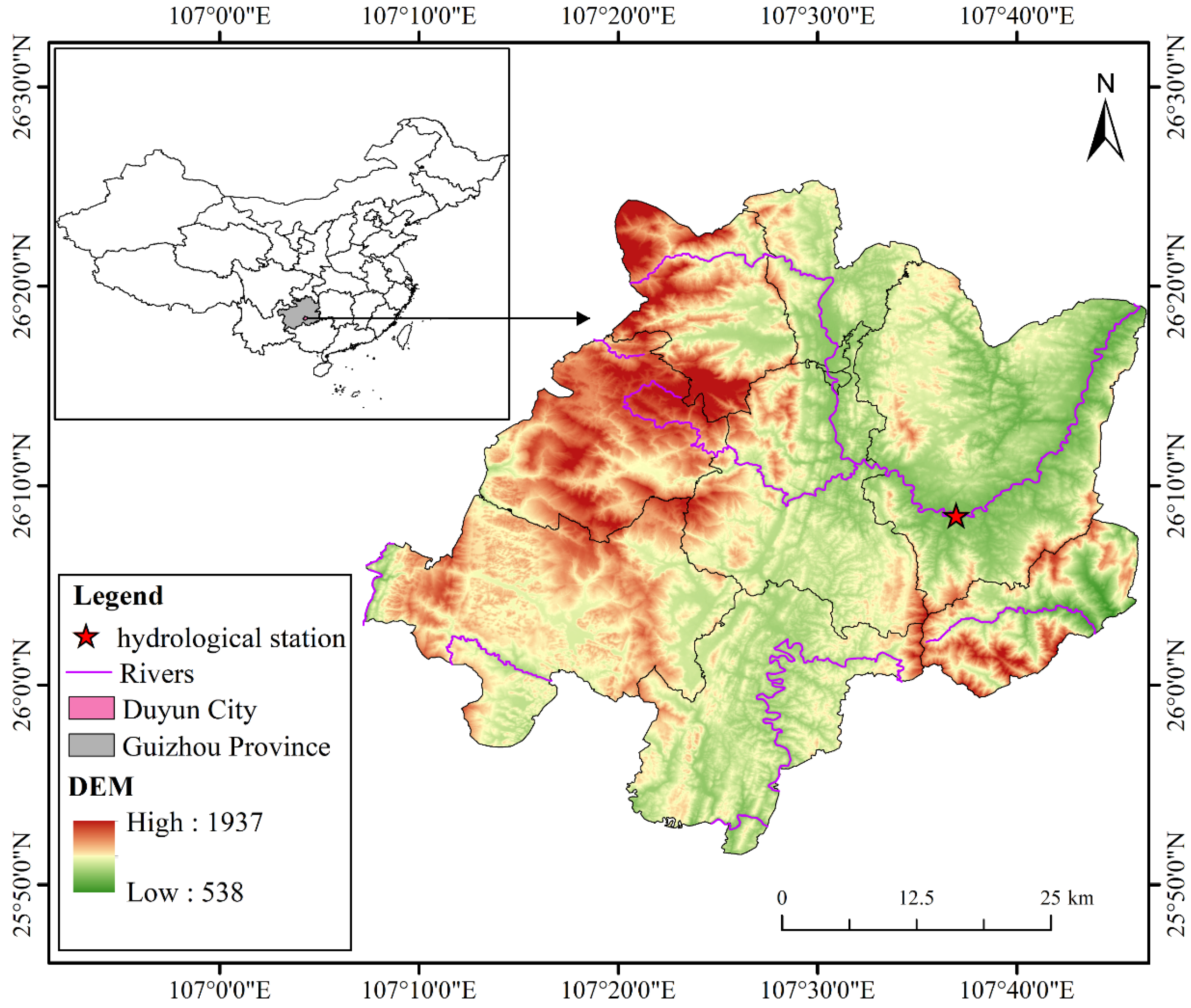
The study area is situated in Duyun City, located in the central-southern part of Guizhou Province, as shown in Figure 2. This region lies on the sloping transition zone between the Yunnan-Guizhou Plateau and the Guangxi Hills, characterized by a terrain that is higher in the north and lower in the south. The climate is diverse, with notable regional and vertical variations, reflecting the typical climate characteristics and variation patterns of plateau mountainous areas [34]. Affected by the East Asian monsoon region, the study area receives abundant heat, with an average annual precipitation of 1300 mm. The rainy season, from April to September, accounts for over 75% of the total annual precipitation [35]. The region experiences significant seasonal temperature fluctuations, exhibiting the typical high-altitude weather characteristics with large diurnal temperature differences [36].

The region offers several distinctive advantages. (1) Climatic representativeness. The region exhibits a pronounced seasonal alternation between hot, humid summers and cool, relatively dry winters, providing an ideal natural setting for investigating the seasonal dynamics of evaporation scale effects. (2) Karst hydrological significance. The area is characterized by typical karst terrain, with thin soils, high permeability, and rapid subsurface drainage. In such environments, surface evaporation plays a particularly critical role in the regional water balance and local water resource management. (3) Operational feasibility. The site hosts a national meteorological and hydrological station equipped with standard E601 and D20 evaporation pans, enabling co-located multi-device monitoring without introducing spatial heterogeneity in environmental conditions. Collectively, these factors make this region uniquely suitable for this research.

2.2. Data Acquisition and Processing

2.2.1. Measurement Protocol and Quality Control

Daily evaporation was measured once per day at 8:00 AM local time using a standard hook gauge with a reading accuracy of ±0.1 mm. This measurement represents the total water loss accumulated over the preceding 24 h period (since the previous day’s reading at the same time). The 8:00 AM observation time was chosen to avoid the thermally unstable periods around midday and sunset, thereby ensuring consistent and comparable daily readings following the standard protocols for pan evaporation observations. To maintain consistent conditions, water levels in all pans were replenished daily to their designated marks after reading. Rainfall events were recorded. If precipitation occurred between readings, the corresponding daily data were discarded to eliminate the direct input effect. A rigorous leakage check was performed weekly for all buried pans. Any data points with suspected leakage or overflow were flagged and excluded from the final analysis, resulting in a valid dataset of over 95% coverage for each device.

2.2.2. Time Scale Aggregation

The research data were obtained by collecting two years of daily evaporation data from five evaporation monitoring devices: D20, E601, P1, P5, and P20. These data were statistically analyzed at annual, seasonal, monthly, and daily scales. Based on this analysis, the E601 evaporation data were used as the reference to examine the correlation and consistency among the different evaporation devices. The seasons were defined as follows: spring from March to May, summer from June to August, fall from September to November, and winter from December to February.

2.2.3. Statistical Analysis Method

The statistics used in this study are mean, maximum, minimum, extreme value, and standard deviation. The formulas are given below.

$$\overline{X}={\displaystyle \frac{1}{n}}{\displaystyle \sum _{i=1}^n{X}_i}$$

(1)

$$X_{\max }=\max (X_1,X_2,\dots ,X_n)$$

(2)

$$X_{\min }=\min (X_1,X_2,\dots ,X_n)$$

(3)

$$\sigma =\sqrt{{\displaystyle \frac{1}{n}}{{\displaystyle \sum _{i=1}^n(X_i-\overline{X})}}^2}$$

(4)

In these equations, σ represents the standard deviation, $\overline{X}$ is the mean, and $X_i$ is the i-th data value. The mean is the arithmetic average of all data values, the maximum value is the largest value in the dataset, the minimum value is the smallest value, and the range (extremes) is the difference between the maximum and minimum values in the dataset. The standard deviation measures the degree of deviation of the data from the mean [37].

2.2.4. Reduction Coefficient

The conversion coefficient can usually be calculated by the following formula:

$$K={\displaystyle \frac{E_{E601}}{E_i}}$$

(5)

where K is the conversion coefficient, $E_i$ is the evaporation monitored in device i, and $E_{\mathrm{E}601}$ refers to the reference evaporation observed by E601 [38].

2.2.5. Correlation Coefficient

In the equation, $X_{o,i}$ represents the observed value, $X_{m,i}$ denotes the corresponding model-predicted value, $\overline{X_{o,i}}$ is the mean of the observed values, and $\overline{X_{m,i}}$ is the mean of the predicted values. The Pearson correlation coefficient is widely used to quantify the degree of linear association between two variables, with values ranging from −1 to 1 [39].

$$r={\displaystyle \frac{{\displaystyle {\sum }_{i=1}^n(X_{o,i}-\overline{X_o})(X_{\mathrm{m},i}-\overline{X_{\mathrm{m}}})}}{\sqrt{{\displaystyle {\sum }_{i=1}^n{(X_{o,i}-\overline{X_o})}^2}}\sqrt{{\displaystyle {\sum }_{i=1}^n{(X_{\mathrm{m},i}-\overline{X_{\mathrm{m}}})}^2}}}}$$

(6)

Monthly correlation coefficients were calculated using daily observations within each calendar month, pooled across the two years (typically 56–62 daily data pairs per month: 2 years × 28–31 days). No overlapping windows were used; each month was treated as an independent window. We emphasize that these monthly patterns describe intra-annual variability observed within the two-year study period and should not be interpreted as long-term temporal trends.

2.2.6. Paired t-Test

A paired t-test was applied to the mean values of the variability indicators (CV, IQR, STD) to assess whether systematic differences in dispersion existed between the devices. The commonly used formulas are as follows:

(1)

Hypothesis Testing

Null Hypothesis H₀: There is no significant difference between the means of the two paired samples, i.e., μ_d = 0.

Alternative Hypothesis H₁: There is a significant difference between the means of the two paired samples, i.e., μ_d ≠ 0.

(2)

Calculation of the Mean and Standard Deviation of the Differences

For each data pair, calculate the difference, and then compute the mean and standard deviation of these differences. The formulas are as follows:

$$d_i=X_{1i}-X_{2i}$$

(7)

$$\overline{d}={\displaystyle \frac{1}{n}}{\displaystyle {\sum }_{i=1}^n{d}_i}$$

(8)

$$s_d=\sqrt{{\displaystyle \frac{1}{n-1}}{{\displaystyle {\sum }_{i=1}^n(d_i-\overline{d})}}^2}$$

(9)

Here, d_i represents the difference for each data pair, X_1i and X_2i are the two paired samples, $\overline{d}$ is the mean of the differences, and s_d is the standard deviation of the differences.

(3)

t-statistic

The t-statistic is used to test whether there is a significant difference between the means of the two paired samples. The formula is as follows:

$$t={\displaystyle \frac{\overline{d}}{s_d/\sqrt{n}}}$$

(10)

In the formula, n represents the number of paired samples.

The degrees of freedom are given by df = n − 1. The calculated t-value is then used to look up the corresponding p-value in the t-distribution table based on the degrees of freedom. This p-value is compared with the significance level to determine whether to reject the null hypothesis. Specifically, if the p-value is less than the significance level, the null hypothesis is rejected, indicating that there is a significant difference between the means of the two paired samples [40].

2.2.7. Correlation Coefficient Trend Analysis

(1)

Estimation of the Trend Slope for z′

Fisher’s z transformation: Given a correlation coefficient r, the corresponding z value is calculated as:

$$z^{\prime }=0.5\ln ({\displaystyle \frac{1+r}{1-r}})$$

(11)

Trend slope: To assess the temporal evolution of the correlation coefficient, a linear regression is applied to the z values over time. The regression model is expressed as:

$$z^{\prime }(t)={\beta }_0+{\beta }_{1}t+\in$$

(12)

where β₁ denotes the trend slope, representing the rate of change in the Fisher-transformed correlation (z) per unit time. This parameter quantifies the long-term tendency of the correlation coefficient in the transformed z domain.

(2)

Calculation of the p-Value

The p-value is derived from the regression model using the t statistic, which evaluates whether the estimated slope differs significantly from zero. The t statistic is given by:

$$t={\displaystyle \frac{{\beta }_1}{SE({\beta }_1)}}$$

(13)

where SE(β₁) is the standard error of the slope estimate. The corresponding p-value can then be obtained from the t distribution table [41]. For the paired t-test, the significance level was set at α = 0.05. The normality of the difference distributions was assessed using the Shapiro–Wilk test. When the normality assumption was violated (p < 0.05), the non-parametric Wilcoxon signed-rank test was applied as a confirmatory analysis. To address the multiple comparison problem arising from 10 device pairs (5 devices × 4 seasons × 3 variability indicators = 120 tests), the Benjamini–Hochberg false discovery rate (FDR) correction was applied at q = 0.05.

The physical interpretation of pan evaporation in this study is grounded in the combination equation originally proposed by Penman (1948) [42], which partitioned evaporation into radiative and aerodynamic components. The subsequent Penman–Monteith formulation [43] further extended this framework by incorporating surface resistance terms, forming the theoretical basis for the energy-balance interpretation adopted in our discussion of seasonal scale-effect reversals.

3. Results

3.1. Multi-Scale Comparison of Evaporation

3.1.1. Annual Evaporation

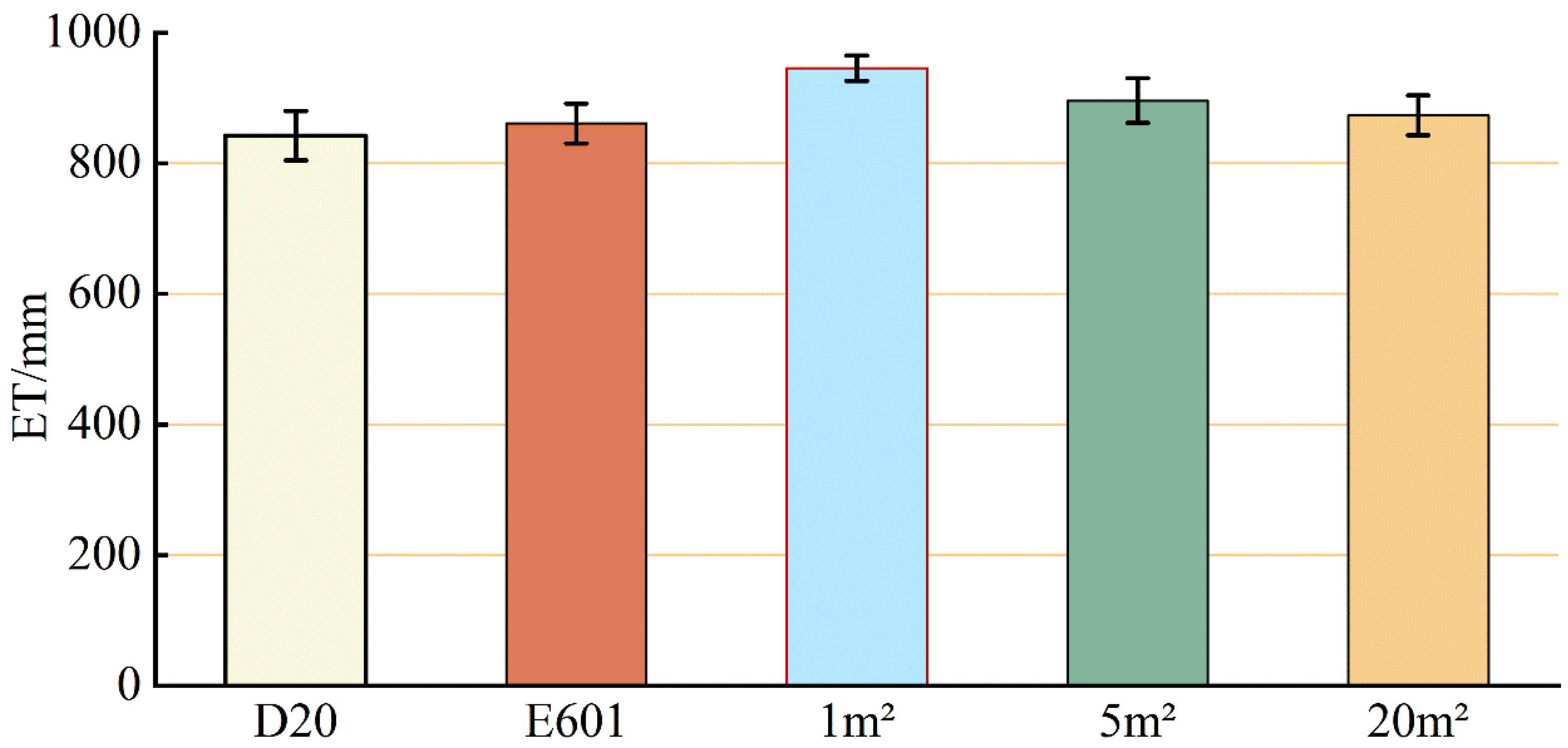
The annual total evaporation amounts observed for five typical devices are shown in Figure 3. The results indicate that the evaporation amounts from the three evaporation ponds are higher than those of the national standard devices, E601 and D20. A comparison of the evaporation amounts from the three evaporation ponds reveals that evaporation decreases as the surface area of the evaporation pond increases, with values of 946 mm, 896 mm, and 874 mm for the P1, P5, and P20 evaporation ponds, respectively. The annual evaporation for E601 is slightly higher than for D20, with corresponding values of 861 mm and 842 mm.

Using E601, the most widely used device in China, as a reference, the conversion coefficients (K) for D20, P1, P5, and P20 are 1.02, 0.91, 0.96, and 0.99, respectively. This indicates that the annual total evaporation amounts for E601, D20, and P20 are similar, with deviations less than 2%. However, the relative deviation in the evaporation amount between E601 and the 1 m² evaporation pond reaches nearly 10%.

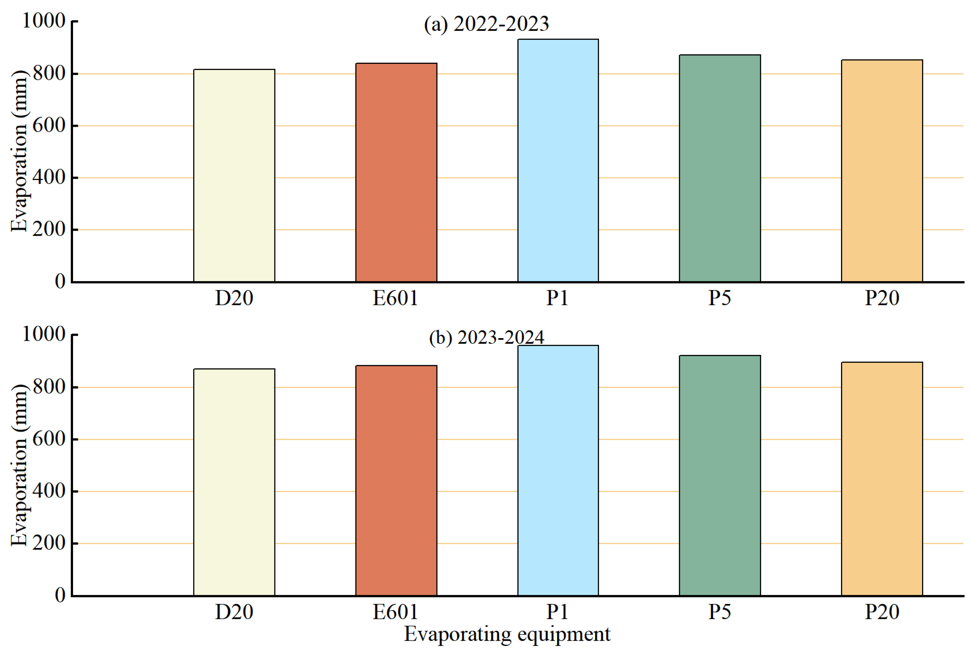
To assess inter-annual stability, Figure 4 presents the annual evaporation for each device in the two years separately. The ranking of the devices remained consistent between years: P1 exhibited the highest evaporation (950 mm in both years), followed by E601, D20, P5, and P20. Among the three ponds, the monotonic decrease in evaporation with increasing surface area (P1 > P5 > P20) was stable across both years. In contrast, D20 and E601 showed greater inter-annual variability, suggesting that their elevated or shallow configurations may be more sensitive to meteorological fluctuations. Despite these differences, the overall pattern was consistent between the two years, supporting the robustness of our main findings.

3.1.2. Seasonal Evaporation

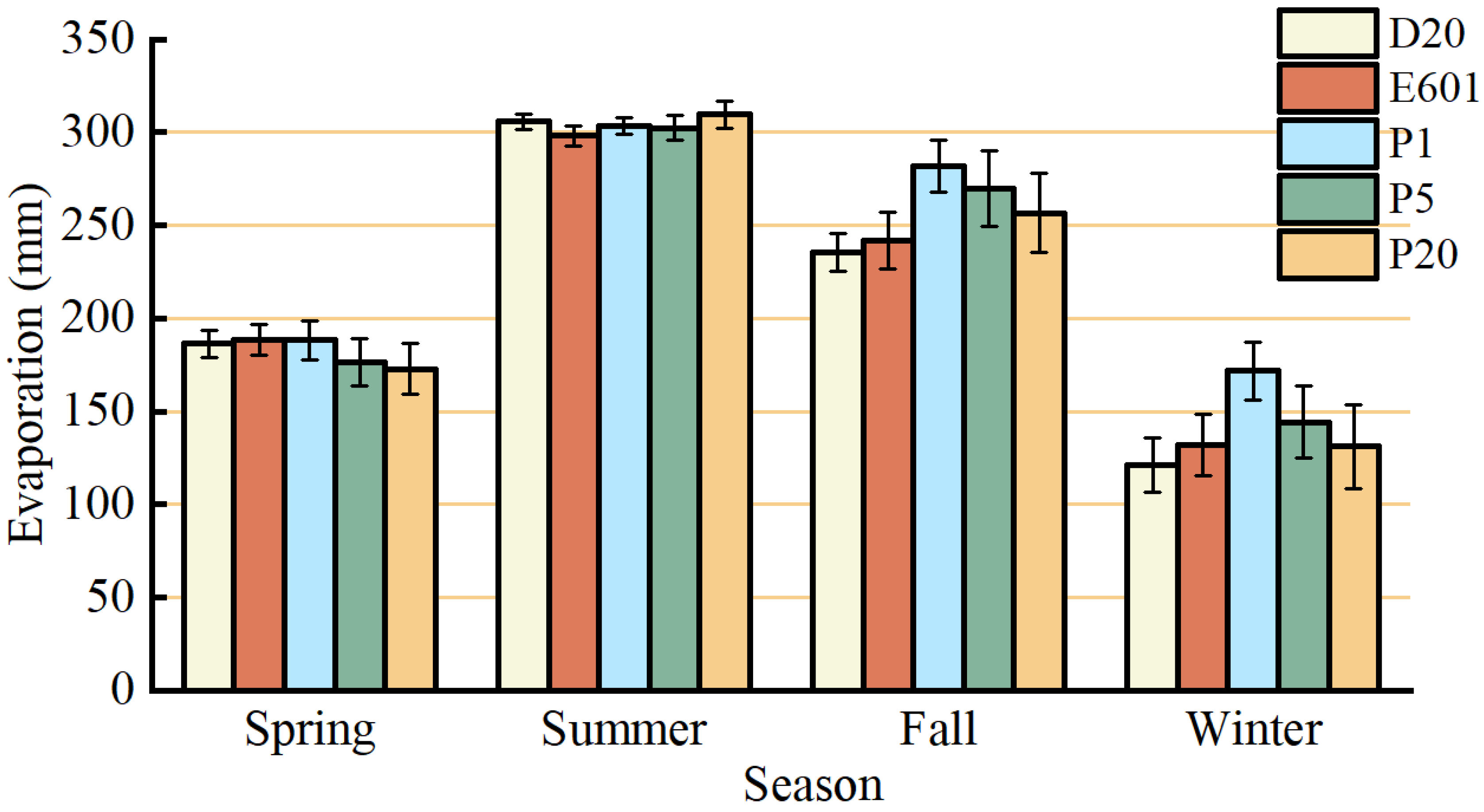
A comparison of the total water surface evaporation amounts measured by the five evaporation monitoring devices in different seasons is shown in Figure 5. The results indicate that the differences in evaporation amounts between the facilities exhibit distinct seasonal characteristics. In spring, the evaporation amounts of D20, E601, and P1 are relatively close, with deviations within 1%, while the evaporation amounts of P5 and P20 are significantly lower. In summer, the evaporation measurements of the five devices are generally consistent, with D20 and P20 showing slightly higher evaporation amounts than the other three devices. In fall and winter, the evaporation amounts follow a similar pattern to the annual totals, with the order being P1 > P5 > P20 > E601 > D20. It can be seen that, although the evaporation amounts are relatively high in spring and summer, the differences in annual total evaporation are mainly determined by the variations in fall and winter, as the coefficients of variation in are 0.07 and 0.14, respectively, while considerably smaller in spring and summer (0.04 and 0.01).

Further analysis reveals that during the summer, the largest evaporation amounts are observed in the large-area evaporation pond P20 and the manually observed D20. In fall and winter, however, evaporation decreases significantly with the increasing size of the evaporation ponds. Notably, in winter, the evaporation amount for P1 exceeds that of E601 by at least 20%, while the observations for the large-area evaporation pond P20 are nearly identical to those of E601. This reflects significant differences in the water–thermal mechanisms, aerodynamic conditions, and other factors between these evaporation facilities across different seasons, which will be discussed further in the following sections.

3.1.3. Monthly Evaporation

(1)

Coefficient of variance among devices

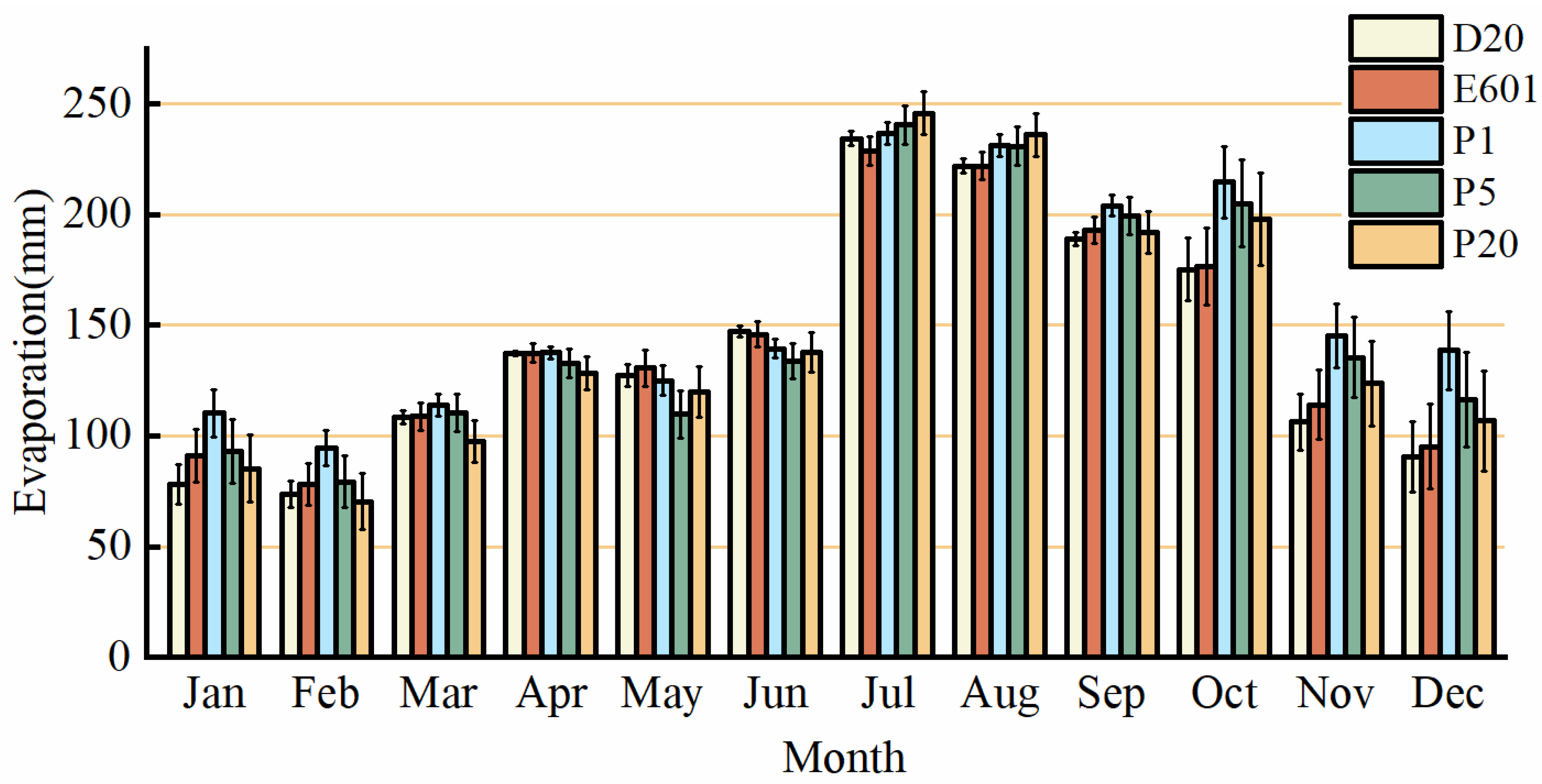
A further analysis of the monthly evaporation differences among the five evaporation devices reveals distinct periodic patterns. The differences among these devices are much smaller from April to September compared to the other six months, with average coefficients of variation (CV) of 0.037 and 0.12, respectively—more than three times larger in the latter period. December exhibits the largest differences, with a standard deviation of 19.13 and a CV of 0.17. The next highest differences are observed in November, January, and February, with CV values exceeding 0.1. In contrast, the CV for evaporation differences among devices is 0.03 in April, June, July, and August.

(2)

Monthly quantitative relationship

Further analysis of the evaporation amount differences among the devices reveals three primary patterns, described as follows.

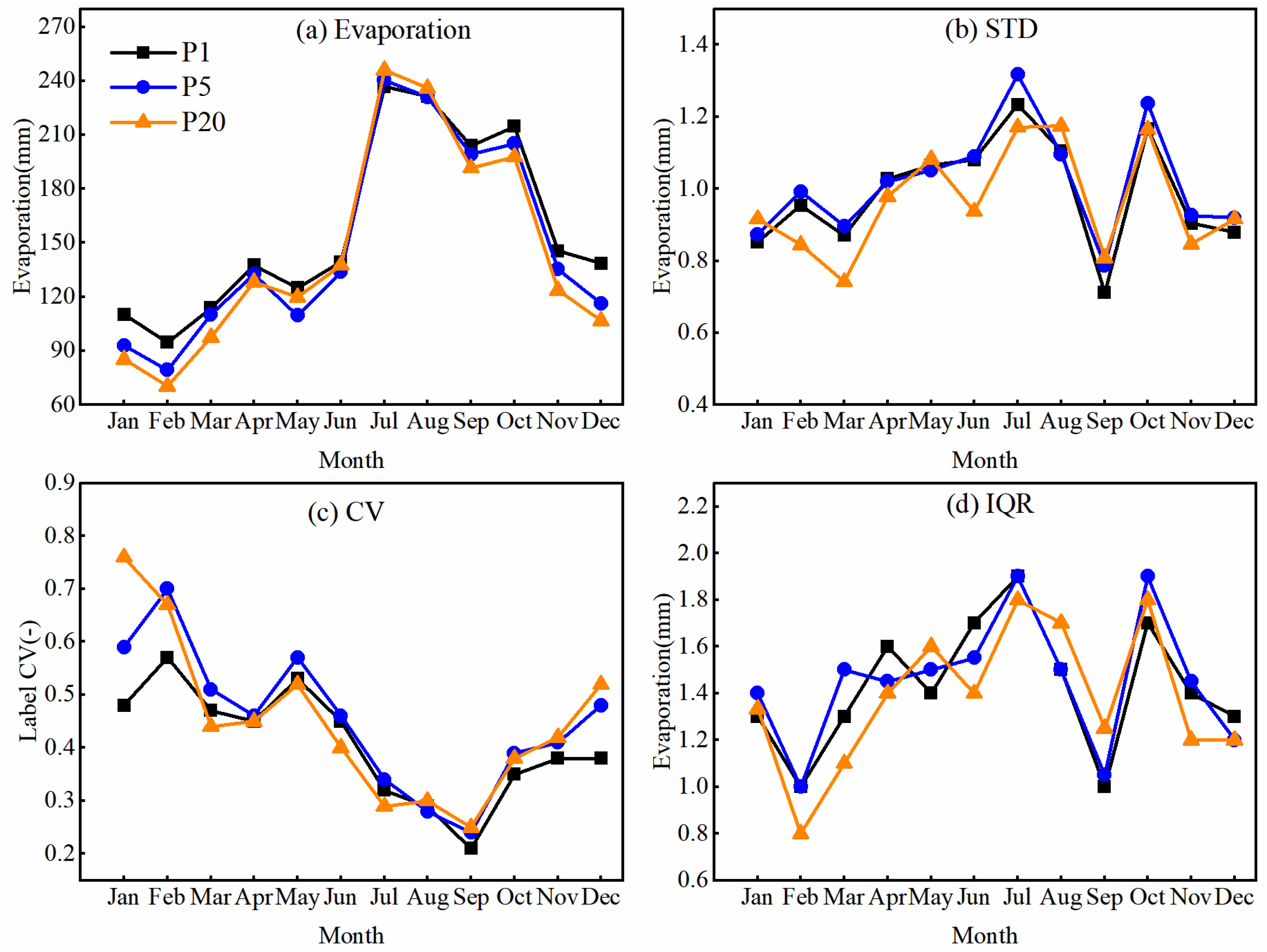
As shown in Figure 6, the monthly evaporation amounts from the three evaporation ponds exhibit clear seasonal differences, divided into three phases. The most prominent phase occurs from September to April of the following year, during which evaporation decreases with increasing surface area, i.e., P1 > P5 > P20. The second typical phase occurs in July and August, showing the opposite trend. The third phase, spanning May and June, shows that the medium-sized pond (P5) displays the lowest evaporation, with P20 being second lowest and P1 being the highest.

The two small evaporation devices, E601 and D20, exhibit similar characteristics to the three evaporation ponds, also following a three-phase pattern. The main phase occurs from September to February of the following year, where E601’s evaporation is higher than that of D20. The second phase, from March to May, shows that D20 and E601 have similar evaporation amounts, with the conversion coefficients (K) ranging from 1.00 to 1.03 (

Table 2. Conversion coefficients (K, mean ± SD) among five evaporation monitoring devices at different time scales, with E601 as the reference. The K values for each period were calculated from daily paired observations. STD and CV refer to the variability of the daily evaporation measurements themselves across devices.

Scale	Sub Scale	E601 (mm)	K (-)				STD	CV
			E601/D20	E601/P1	E601/P5	E601/P20	(mm)	(-)
Annual	Annual	861.1	1.02 ± 0.05	0.91 ± 0.04	0.96 ± 0.05	0.99 ± 0.04	39.72	0.04
Seasonal	Spring	188.4	1.01 ± 0.04	1.00 ± 0.05	1.07 ± 0.06	1.09 ± 0.05	7.35	0.04
	Summer	301.9	0.99 ± 0.03	0.98 ± 0.03	0.98 ± 0.04	0.96 ± 0.03	4.27	0.01
	Fall	241.35	1.03 ± 0.07	0.86 ± 0.06	0.90 ± 0.07	0.94 ± 0.06	19.26	0.07
	Winter	132.3	1.09 ± 0.09	0.77 ± 0.08	0.92 ± 0.10	1.01 ± 0.08	19.49	0.14
Monthly	Jan	91.1	1.17 ± 0.11	0.83 ± 0.07	0.98 ± 0.09	1.07 ± 0.08	11.97	0.13
	Feb	78.2	1.06 ± 0.10	0.83 ± 0.06	0.99 ± 0.07	1.11 ± 0.09	9.31	0.12
	Mar	108.8	1.00 ± 0.05	0.96 ± 0.05	0.99 ± 0.04	1.12 ± 0.06	6.14	0.06
	Apr	137.4	1.00 ± 0.04	1.00 ± 0.04	1.04 ± 0.05	1.07 ± 0.05	4.11	0.03
	May	130.6	1.03 ± 0.06	1.04 ± 0.06	1.19 ± 0.08	1.09 ± 0.06	8.14	0.06
	Jun	145.8	0.99 ± 0.04	1.05 ± 0.05	1.09 ± 0.06	1.06 ± 0.05	5.68	0.04
	Jul	228.7	0.98 ± 0.03	0.97 ± 0.04	0.95 ± 0.04	0.93 ± 0.04	6.42	0.03
	Aug	221.9	1.00 ± 0.04	0.96 ± 0.04	0.96 ± 0.04	0.94 ± 0.04	6.26	0.03
	Sep	192.9	1.02 ± 0.05	0.95 ± 0.05	0.97 ± 0.05	1.01 ± 0.05	6.07	0.03
	Oct	176.6	1.01 ± 0.08	0.82 ± 0.07	0.86 ± 0.08	0.89 ± 0.07	17.43	0.09
	Nov	114.1	1.07 ± 0.10	0.78 ± 0.09	0.84 ± 0.09	0.92 ± 0.08	15.75	0.13
	Dec	95.1	1.05 ± 0.12	0.69 ± 0.10	0.82 ± 0.11	0.89 ± 0.09	19.13	0.17

Notes: The standard deviations of the conversion coefficients, calculated from daily K value distributions, are shown as “±” values in Table 2. The corresponding 95% confidence intervals are provided in Supplementary Table S1.

). The third phase, from June to August, shows that the evaporation from E601 is slightly higher than that of D20.

When comparing the measurements of the evaporation ponds and small evaporation devices together, four distinct patterns are observed. Pattern 1, observed from October to December, shows the characteristics of a higher evaporation in the three ponds while lower in the small evaporation devices, and the evaporation substantially decreases with surface area of the three ponds. Pattern 2, observed in July and August, shows the evaporation increase with the expansion of the surface area. Pattern 3 happens during April to June, shows a larger evaporation in D20 and E601, and P5 exhibits the least evaporation (P1 > P20 > P5). Pattern 4 occurs in January, February, March, and September and represents a mixed pattern. During these months, P1 consistently records the highest evaporation among the five devices, while the evaporation from E601 and P5 are similar to each other, and D20 and P20 also show similar values—the latter being noteworthy given their substantial difference in surface area.

3.2. Variability of Monitoring Results

3.2.1. The Overall Difference

A paired t-test is conducted to analyze the overall difference of the three fluctuation indices for the observation data between any two devices; the results are shown in

Table 3. Results of paired test for three indicators.

Indicator	Device	Tstat				H				p-Value
		D20	P1	P5	P20	D20	P1	P5	P20	D20	P1	P5	P20
CV	E601	5.23 **	3.88 **	0.48	0.31	1	1	0	0	0.0003	0.0026	0.64	0.77
	D20	-	−0.24	−3.92 **	−1.63	-	0	1	0	-	0.82	0.0024	0.13
	P1	-	-	−3.70 **	−1.64	-	-	1	0	-	-	0.0035	0.13
	P5	-	-	-	0.11	-	-	-	0	-	-	-	0.92
IQR	E601	6.61 **	0.42	0.00	1.10	1	0	0	0	0.00	0.68	1.00	0.29
	D20	-	−2.45 *	−2.63 *	−1.77	-	1	1	0	-	0.03	0.02	0.10
	P1	-	-	−0.74	0.78	-	-	0	0	-	-	0.48	0.45
	P5	-	-	-	1.33	-	-	-	0	-	-	-	0.21
STD	E601	7.19 **	0.79	−0.19	1.05	1	0	0	0	0.000018	0.45	0.85	0.32
	D20	-	−3.89 **	−4.60 **	−2.32 *	-	1	1	1	-	0.0025	0.0008	0.04
	P1	-	-	−3.09 *	0.94	-	-	1	0	-	-	0.01	0.37
	P5	-	-	-	2.09	-	-	-	0	-	-	-	0.06

Notes: Significance level: α = 0.05. Statistical significance was assessed using two-tailed paired t-tests (df = 11 for all comparisons). * indicates significance at p < 0.05 after Benjamini–Hochberg FDR correction (q = 0.05); ** indicates significance at p < 0.01 after FDR correction. T-statistics are shown; negative t-values indicate that the first device in the pair has lower variability than the second. H = 1 indicates rejection of the null hypothesis at q = 0.05 after FDR correction.

. It can be observed that the volatility indices (CV, IQR, STD) of E601 are significantly higher than that of D20, and the T statistics for the CV, IQR, and STD indicators all exceed the highly significant level of 0.01. The three fluctuation indices for D20 also exhibit values lower than P5, with results reaching the significant level of 0.01. Additionally, its IQR and STD are significantly lower than those of P1, although the CV did not reach the 0.05 significance level.

Comparisons between the three evaporation ponds show that the volatility indices of P1 are lower than that of P5, with paired test statistics for all three indicators being negative. Both the CV and STD reach significant levels, while the t-statistic for the IQR is −0.76. Meanwhile, the volatility indices of P5 are higher than that of P20, with positive t-statistics for all indicators, but none of them reached the 0.05 significance level. The closest is STD, with a t-statistic of 2.09, just below the critical value of 2.10. Thus, based on the statistical differences among the three evaporation ponds, it can be concluded that P5 exhibited the highest average volatility indices, indicating that the daily evaporation at P5 showed the greatest degree of dispersion among the three evaporation pans, followed by P20, while P1 displayed the lowest volatility.

A comprehensive analysis of the variability in the monitoring results of the five devices reveals that E601 has the highest volatility indices, with its statistics being positive relative to all other devices. D20 exhibits the lowest volatility, with its statistics negative relative to all other device observations. The middle range is as follows: P5 > P1 > P20. Accordingly, the overall volatility level followed the order: E601 > P5 > P1 > P20 > D20, based on pairwise tests of the mean values of each volatility metric.

Prior to performing the paired t-tests, the normality of difference distributions was examined using the Shapiro–Wilk test. For the majority of device pairs (78 out of 120, or 65%), the normality assumption was satisfied (p > 0.05). For the remaining pairs where normality was violated, Wilcoxon signed-rank tests confirmed the same significance patterns as the paired t-tests, indicating that the t-test results are robust to minor deviations from normality. The results reported in Table 3 are based on paired t-tests with FDR-corrected significance levels

3.2.2. Dynamic Differences of Variability

(1)

Seasonal characteristics

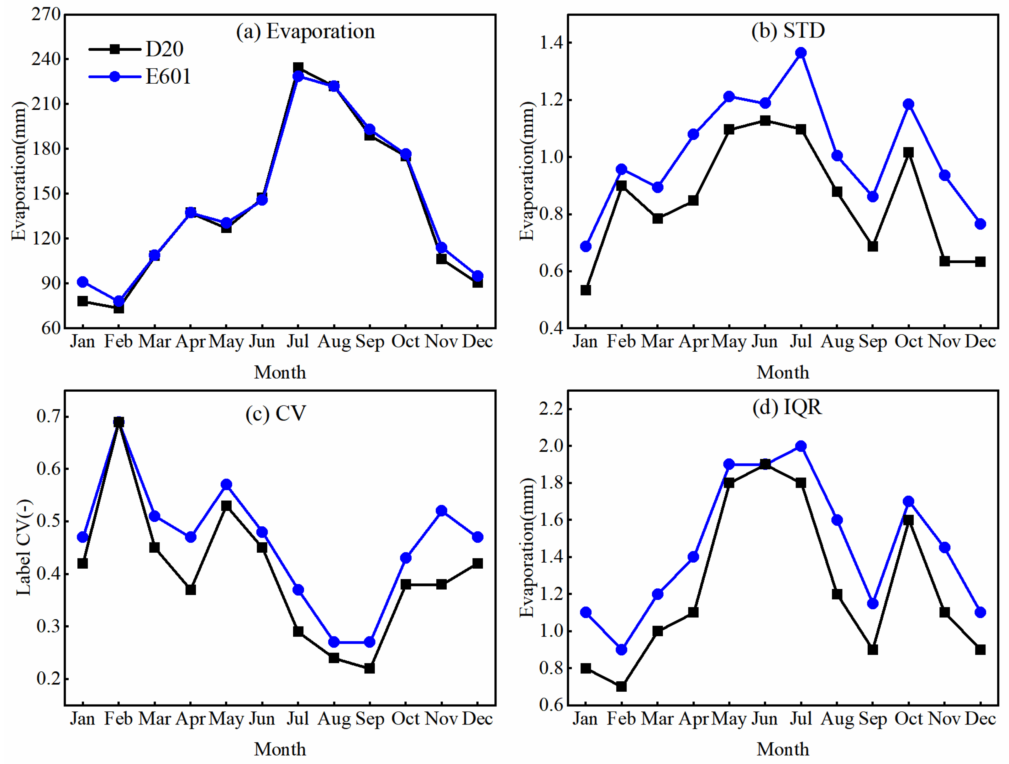
The variations of three data based on three indicators of IQR, STD, and CV throughout the year are depicted in Figure 7 and Figure 8. It is evident that all three variables exhibit a distinct annual periodicity, but there are clear differences among them. Both IQR and STD show an M-shaped double-period pattern, with the first period spanning from February to September, and the second period extending from September to February of the following year. In contrast, CV displays a V-shaped single-period pattern (from February to January), with a notable abnormal spike in May, followed by a steady decline until reaching the minimum in September, after which it gradually increases again.

(2)

Differences between variables

The variability indicators of evaporation obtained from different monitoring devices exhibit significant variations across different seasons. Among them, three indicators show consistency between the two small-scale evaporation monitoring devices, with the higher value in E601 than those of D20, as shown in Figure 6.

For the three evaporation ponds of different sizes, the coefficient of variation (CV) of evaporation data in different months exhibits two distinct patterns. From September to January, the coefficient of variation increases with the water surface area. From March to July, P5 shows the highest variation, followed by P1, with P20 exhibiting the smallest variation. February and August serve as transition months, with the variation characteristics falling between the two patterns. As for IQR and STD, no obvious regularity is observed in the differences among the three evaporation ponds, indicating significant randomness.

3.3. Correlation Analysis

3.3.1. Comparison Among Monitoring Devices

(1)

Seasonal evaporation

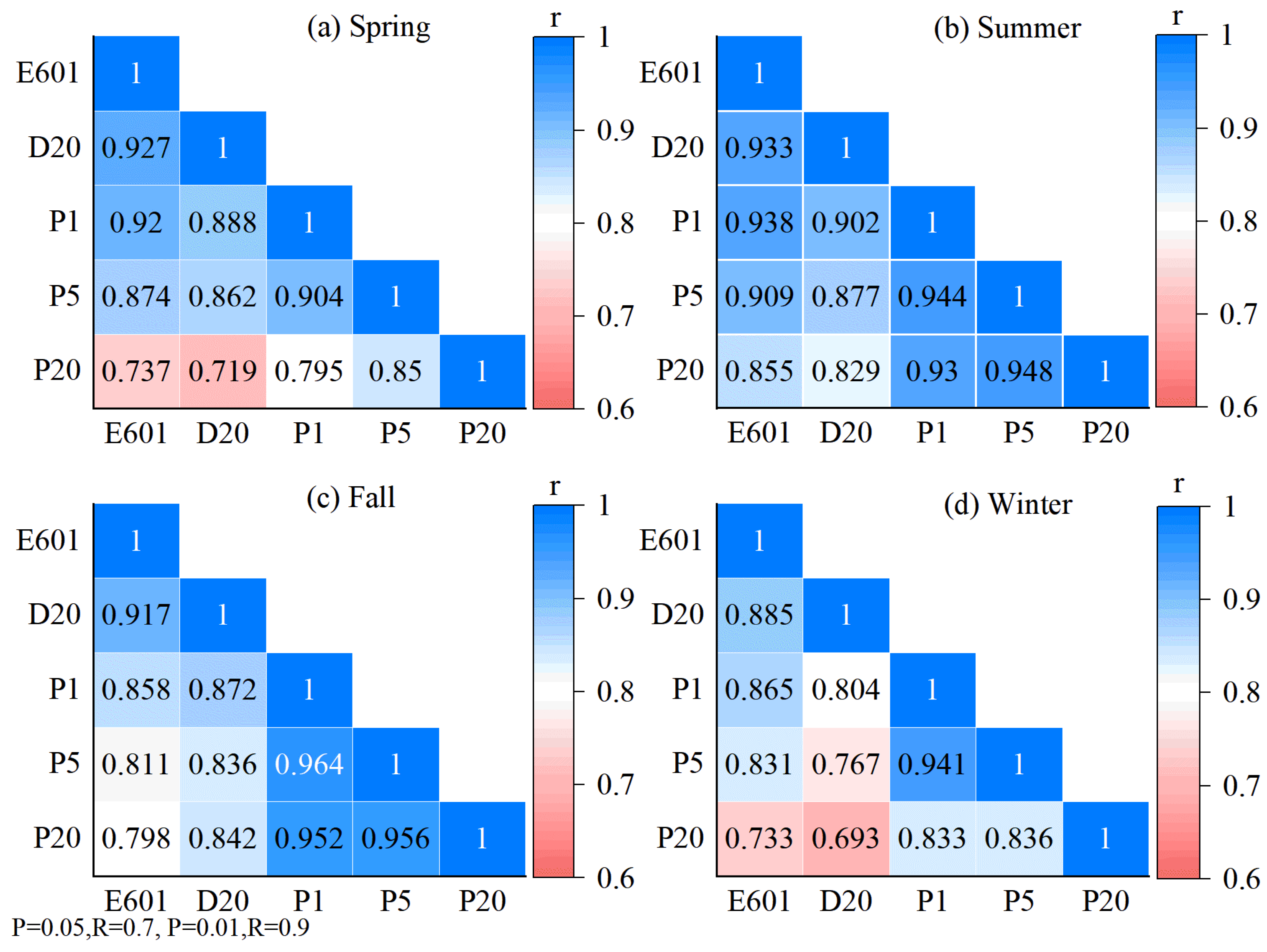
The correlation coefficients of evaporation data observed by any two facilities in different seasons are analyzed and visualized in a heatmap, as shown in Figure 9. The results reveal significant differences in the correlation based on large and small evaporation devices, which also exhibit strong seasonal variations. The linear correlation between the small-area evaporation device D20 and E601 is particularly strong, with maximum correlation observed in all four seasons. For medium and large evaporation devices, such as P1, P5, and P20, strong linear correlations are also evident, and the correlation improves as the evaporation pond area increases. When analyzing pairs of different-sized devices, the correlation coefficient significantly decreases, and the larger the area difference, the greater the reduction in correlation. Regarding seasonal characteristics, the correlations are generally highest in summer, followed by fall and spring, with the lowest in winter. In summer, the correlation coefficient ranges from a minimum of 0.829 (D20 vs. P20) to a maximum of 0.948, whereas in winter, it drops to a minimum of 0.693 and peaks at only 0.885.

(2)

Monthly evaporation

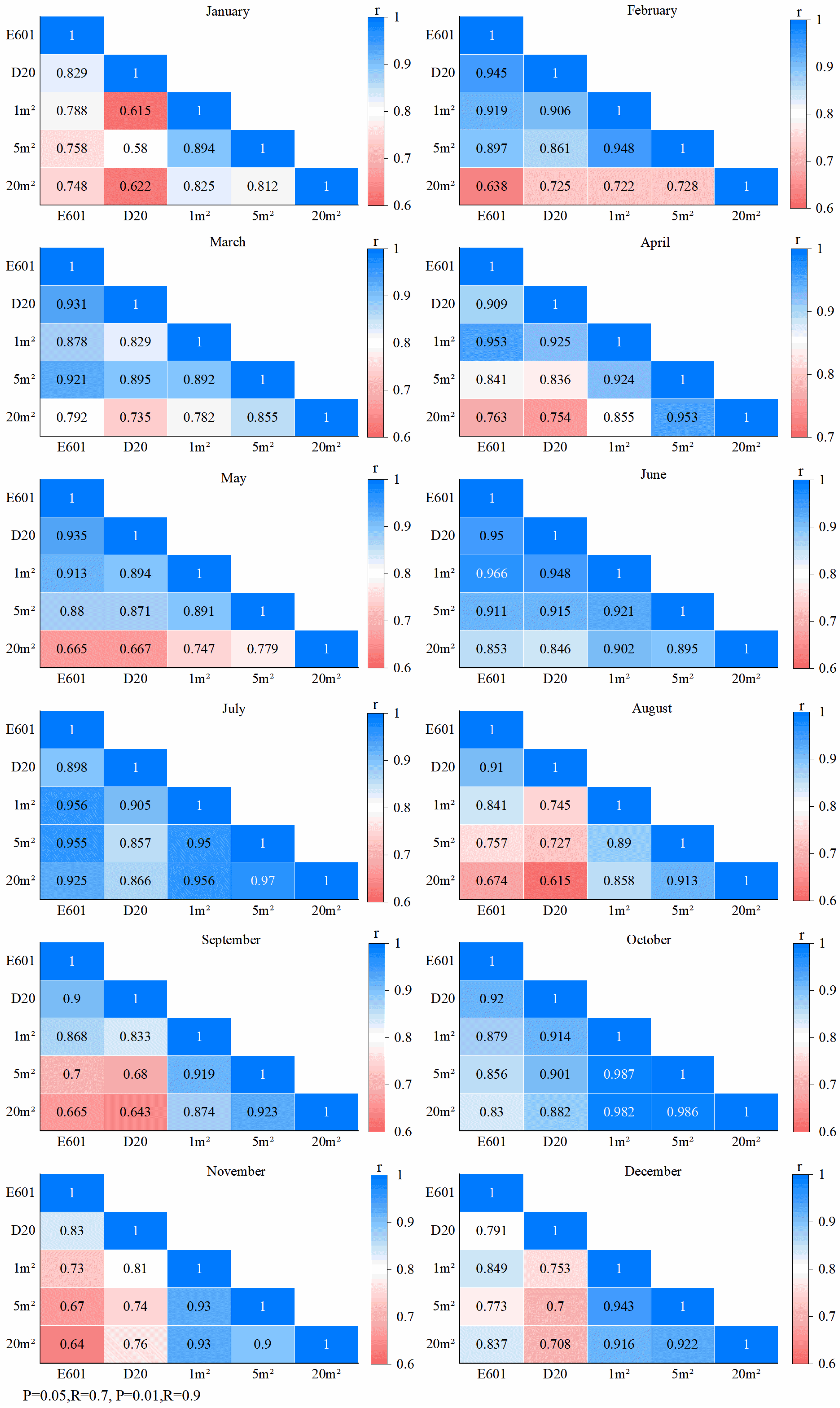
Further analysis of the daily evaporation amounts observed by any two devices for each month, as shown in Figure 10, reveals overall patterns consistent with the seasonal analysis, while also highlighting two distinct differences. On one hand, the correlation between measurements from different evaporation devices fluctuates more significantly on a monthly scale, with a broader range of variation. For instance, the correlation between D20 and the three evaporation ponds is as low as 0.58, notably lower than the seasonal correlation of 0.693. On the other hand, the maximum correlation coefficient between P20 and P5 monitoring data can reach as high as 0.986. Although the overall correlations among all device pairs are highest during summer and autumn, there is a notable exception: in August, September, and November, the correlations between the two small pans (E601, D20) and the three large ponds (P1, P5, P20) decrease substantially, dropping from values above 0.8 to a range between 0.6 and 0.8.

3.3.2. Monthly Correlation Dynamics

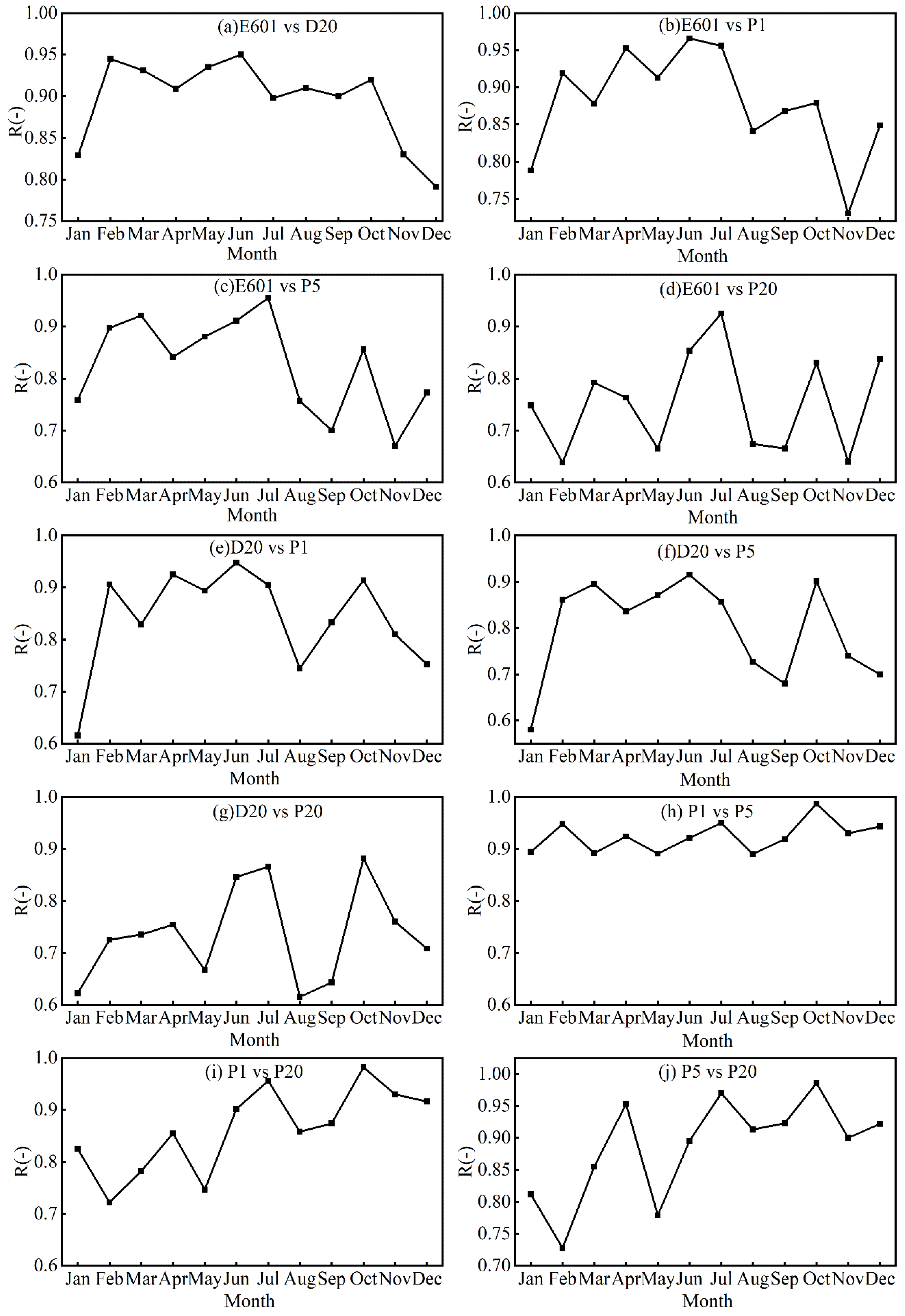
The monthly patterns of correlation coefficients between different evaporation facilities are analyzed, as shown in Figure 10. It is evident that the evaporation data exhibit different seasonal characteristics between small-scale evaporation devices, evaporation ponds, and between small-scale devices and ponds, as described below. These patterns reflect intra-annual variability observed during the two-year study period.

(1)

Between E601 and D20

The correlation coefficients of the observation data from the small evaporation devices E601 and D20 exhibit a distinct periodic pattern, with consistently high values from February to October, and a significant decrease from November to January, as shown in

Table 4. Time mode of R between different evaporation monitoring systems.

Monitoring System	Period		Mean
	High R	Low R	High R	Low R
E601 vs. D20	Feb–Oct	Nov–Jan	0.922	0.82
E601 vs. P1	Feb–Jul	Aug–Jan	0.93	0.83
E601 vs. P5	Feb–Jul	Aug–Jan	0.90	0.75
D20 vs. P1	Feb–Jul and Oct	Aug–Jan except Oct	0.90	0.75
D20 vs. P5	Feb–Jul and Oct	Aug–Jan except Oct	0.88	0.69

. The average correlation coefficients for these two periods are 0.922 and 0.82, respectively, with the former being 11.1% higher than the latter.

(2)

Among evaporation ponds

The correlation coefficients among the observation values of the three evaporation ponds with different surface areas are shown in Figure 11h–j. The monthly correlation patterns do not exhibit a distinct seasonal periodicity for the pond-to-pond comparisons; rather, they show a gradual increase from January to December (Figure 11h–j), reflecting a within-year pattern rather than a long-term trend. The minimum value is generally observed in February, while the maximum occurs in November. We performed linear regression on the correlation coefficient series after Fisher’s z-transformation, and the results are presented in

Table 5. Linear trend for temporal patterns of R among different evaporation monitoring systems.

Monitoring System	Slope of z′	p-Value
P1 vs. P5	0.034	0.189
P1 vs. P20	0.076	0.018
P5 vs. P20	0.068	0.064
E601 vs. P20	0.010	0.671
D20 vs. P20	0.015	0.463

. The estimated slopes of z′ were 0.034, 0.076, and 0.068 for P1–P5, P1–P20, and P5–P20, respectively, with corresponding p-values of 0.189, 0.018, and 0.064. These results indicate that the correlations between P1 and P20, as well as between P5 and P20, exhibited a statistically significant increasing trend over time.

(3)

Between small-scale evaporation devices and evaporation ponds

The correlation coefficients of monthly monitoring data between the two small-scale evaporation devices and the three evaporation ponds are shown in Figure 11b–g. The results show that the correlation between E601, D20, and the evaporation ponds P1 and P5 shows clear seasonal variation, while the correlation with P20 exhibits a gradual increasing trend. However, this periodicity differs from the correlation between the two small-scale devices, E601 and D20. E601 shows consistently high correlation from February to June, followed by a relatively low correlation from July to January. D20 follows a similar pattern, with an exception in November, where the correlation is notably high. In terms of trend, the rate of increase between E601 and P20 is relatively low; whereas for D20 and P20, the rate of increase rises to 0.015, with a p-value of 0.463. It is important to note that the correlation coefficients for both devices are relatively low in August and September, reflecting significant differences in the thermodynamic properties between the evaporation facilities.

To examine whether geometric similarity affects the synchrony of evaporation among different devices, the surface-area difference index $D_a=\left|\mathrm{l}\mathrm{n}\right(A_i/A_j\left)\right|$ and the corresponding daily correlation coefficients (r) were calculated for all device pairs (

Table 6. Pairwise relationships between geometric similarity and daily evaporation correlation for different evaporation devices.

Device Pair	Da	r
E601–D20	2.253	0.94031
E601–P1	1.204	0.9125
E601–P5	2.813	0.89354
E601–P20	4.605	0.8319
D20–P1	3.46	0.88588
D20–P5	5.07	0.88202
D20–P20	6.456	0.84354
P1–P5	1.609	0.95392
P1–P20	2.996	0.88869
P5–P20	1.386	0.91462

).

The results show that pairwise correlations generally decrease with increasing $D_a$. Among the three evaporation ponds with identical structural configuration (P1, P5, and P20), correlation coefficients decrease from 0.95392 (P1–P5) to 0.91462 (P5–P20) and 0.88869 (P1–P20), indicating a clear dependence of evaporation synchrony on surface-area similarity under controlled design conditions.

4. Discussion

4.1. Physical Mechanisms of Evaporation Difference at Multi-Scale

The study reveals that the annual evaporation pattern (P1 > P5 > P20) is consistent with the well-recognized scale effect [44,45], while the seasonal reversals are less frequently reported. However, the mechanistic interpretation below is constrained by the lack of direct measurements of water temperature and near-surface wind profiles. The following discussion therefore distinguishes between observed patterns and inferences based on physical principles.

For the three evaporation ponds with different surface areas, the monthly evaporation rates exhibit significant differences during the cold season (September to April), transition season (May to June), and hot season (July to August). The key characteristic of the cold season is that evaporation decreases as the surface area increases. A plausible explanation is that smaller evaporation ponds, with their larger specific surface areas, may receive more heat from the ground during the night, which would tend to sustain evaporation [46]. In the dry hot season, this trend reverses. On one hand, the water absorbs more solar radiation than the vegetated turf, and the intense radiation and higher air temperature may cause the surface water temperature to be significantly higher than the ground temperature. This would make larger devices, with their larger surface area and thermal inertia, more likely to accumulate heat during day and night, thus potentially maintaining higher water temperatures [47]. On the other hand, it is reasonable to infer that the resistance of the evaporation pond’s sidewalls to wind speed decreases with increasing water surface area, which would further enhance evaporation [48,49]. During the transition season, the observed evaporation pattern (P1 > P20 > P5) may result from the distinct and differently weighted influences of wind speed and ground temperature on the three evaporation devices. P1 has the highest evaporation rate and the lowest surface wind speed, which may indicate that heat exchange in this period is primarily driven by ground temperature. Further analysis shows that P20 receives the lowest heat supply from the ground, and its evaporation rate exceeds that of P5, suggesting that the impact of wind speed is significantly stronger during this period. In contrast, P5 may exhibit weaker combined effects of ground temperature and wind speed during the night, due to the nonlinear effects of the sidewalls on wind speed [50]. Both small-scale evaporation devices also exhibit similar seasonal reversal characteristics. Previous studies have shown that the conversion coefficient range of small-scale evaporation pans, such as D20 and E601, on an annual scale is between 0.55 and 0.80, emphasizing that radiation or air temperature is the main driving force of evaporation from small-scale pans [51]. In this study, the conversion coefficient range between the small-scale evaporation devices is between 0.85 and 1.05, which is higher than the values reported in previous studies. In addition, the study suggests that besides radiation, air temperature, and wind speed, factors such as thermal inertia, sidewall effects, installation position, and material also significantly affect the evaporation rate of small-scale evaporation pans.

The evaporation dynamics of the P20 exhibit partial similarity to natural lakes discussed in Han and Guo [44], particularly regarding thermal inertia. However, its limited fetch likely restricts the full development of advective processes and boundary-layer effects characteristic of larger water bodies, as noted in studies like Workie et al. [52]. This distinction highlights the scale-dependent transition from pan-to lake-like evaporation physics.

A comparison between the small-scale evaporation pans and the three evaporation ponds reveals two key aspects for further discussion. First, from April to June, the evaporation rate of the small-scale evaporation pans, E601 and D20, is higher than that of the three evaporation ponds. This suggests that during this period, E601 may experience stronger ground temperature heat supply, while D20’s higher evaporation rate is primarily due to more intense atmospheric heat exchange, likely because of its metal material with higher thermal conductivity [53]. Second, in some months of the cold season, the observation values of the small-scale evaporation pans are nearly identical to those of certain evaporation ponds, such as D20 with P20 and E601 with P5. However, the reasons for these similarities may differ. The similarity between D20 and P20 may be partly attributable to stronger heat exchange from air temperature for D20, while P20’s evaporation appears to be more strongly influenced by wind speed. For E601 and P5, the similarity could arise because of greater potential ground temperature heat supply for E601, while P5 receives less ground heat supply, but its evaporation rate may be enhanced by wind speed. The interpretation of observed evaporation differences, such as those during April–June and the cold season, therefore requires integrating the scale effect with the design effect arising from installation methods.

4.2. The Differences of Correlation Among the Data

This study, through a multi-time-scale systematic analysis, explores the dynamic differentiation characteristics of the linear correlation between the observed values of evaporation devices at different scales and their potential dominant physical mechanisms.

(1)

Differences Between Devices

The study shows that the correlation between data from different evaporation facilities varies significantly, with the correlation being better when the shape and area differences between devices are smaller. The overall correlation coefficients between the three evaporation ponds and between E601 and D20 are high (average 0.90), with P1 and P5 showing the highest overall correlation (average 0.92). The correlation between E601 and the evaporation ponds is better, significantly higher than that between D20 and the ponds. It should be noted that inter-device correlation tends to increase with geometric similarity, suggesting a dependence of evaporation synchrony on surface-area consistency [54]. This appears to be associated with the combined influence of water–thermal processes, wind speed driving factors, and other variables that collectively determine evaporation dynamics [55,56,57]. The heat conduction equation indicates that the transfer of heat from high to low-temperature objects is a nonlinear process [58], and the impact of near-ground sidewalls on wind speed is also understood to be nonlinear [59]. Therefore, when there are significant structural and size differences between evaporation facilities, the observed values may not strictly follow a linearly scaled relationship, but rather tend toward a nonlinear one; conversely, when the differences are minimal, the relationship can be approximated as linear.

(2)

Seasonal Characteristics

The study reveals that the linear strength of the evaporation relationship is not only significantly constrained by the device scale (area) but also exhibits strong seasonal and time-scale dependence. During the summer, correlation coefficients for all device combinations peak, typically exceeding 0.85. This suggests that under high temperature and strong solar radiation conditions, the dominant driving forces governing evaporation become more consistent across differently scaled devices [60], which would leading to a more uniform evaporation process and a stronger linear relationship among measurements. The high consistency observed across all devices during summer can be understood within a broader context. Under energy-sufficient conditions characterized by high temperature and solar radiation, the primary drivers of evaporation converge, leading to a homogenization of the process across different scales [61]. This dominant energy forcing overwhelms the distinctive effects of pan size and design, which likely results in the strong linear correlations observed. In spring and fall, the correlation is somewhat lower, with r values mostly ranging from 0.75 to 0.95, which may reflect slight disturbances in the consistency of the evaporation process due to increased meteorological variability in transitional seasons. In winter (December to February), a significant decline in correlation is observed, especially for large devices (20 m²), where the correlation with other devices drops dramatically. For example, the correlation between the 20 m² device and D20 drops from 0.842 in fall to 0.693 in winter, a decrease of 17.7%. This decline may be closely related to the transition of the dominant heat source from solar radiation to soil heat flux during the cold season [62], amplified differences in thermodynamic responses between devices, and the enhanced nonlinearity in latent heat distribution processes [63], which would lead to severe differentiation in evaporation dynamics across device scales.

Further analysis of the monthly daily evaporation correlations shows that for small-scale evaporation pans, the correlation is high from February to October and low from November to February. For the three evaporation ponds, the correlation increases with fluctuations from January to December. The correlation between small-scale evaporation pans and evaporation ponds P1 and P5 is high from February to July and in October, with lower correlations in the other months. The correlation between P20 and both E601 and D20 decreases, and its seasonal characteristics are not as pronounced. A possible reason is that, during the radiation-dominated warm season, medium to large water bodies, sharing similar heat accumulation and release mechanisms [64], exhibit synchronized evaporation processes, while smaller devices, which respond more quickly and are more susceptible to instantaneous meteorological disturbances, show some degree of divergence in their dynamics [65,66,67].

4.3. Variability Levels and Driving Factors

(1)

Driving factors identification

The results indicate that the data variability of the five evaporation monitoring devices is highest for E601 and lowest for D20, with both showing statistical significance. The three evaporation ponds fall in between, with the order being P5 > P1 > P20. For the three evaporation ponds, the patterns suggest that, in the water-heat processes associated with land and water evaporation, the dominant factors for P1 and P20 are relatively simple, namely temperature and wind speed, respectively. In contrast, P5 exhibits more complex seasonal characteristics in the dominant factors of both processes, leading to higher variability. D20, due to its significantly higher sidewalls and smaller surface area, experiences minimal impact from air movement [68], and its evaporation is primarily determined by heat balance, resulting in the lowest variability. E601, which appears to be affected by a combination of solar radiation, ground temperature, and wind speed, shows higher variability in its monitoring results, with significance at the 0.01 level. This may be partly attributable to E601’s shallower water depth [69], which is considerably lower than the 3 m depth of the evaporation ponds, potentially making it more responsive to radiative forcing [70]. Its water surface, which is higher than the surrounding environment, may experience higher wind speeds, as wind speed increases nonlinearly with height near the ground [71].

(2)

Season patterns

In this study, all three statistical indicators exhibit clear annual periodicity. IQR and STD, as measures of the absolute fluctuation amplitude of daily evaporation, show a typical bimodal structure (M-shape) in their annual variation, with peaks occurring in spring (March to May) and fall (September to November), and troughs in summer (July to August) and deep winter (January). These phenomena are likely due to the significant fluctuations in meteorological elements (radiation, temperature, humidity, wind speed) during the transitional seasons of spring and fall [72]. In spring, increased radiation is accompanied by frequent cold air activities, and the significant diurnal and interdaily meteorological variations in karst regions [73] may enhance evaporation fluctuations. In fall, while radiation decreases, wind speed increases, and cold fronts cause abrupt temperature changes. These factors may intensify the absolute fluctuations in daily evaporation. During summer, high temperatures and intense radiation dominate [55], which would lead to a stable energy supply with minimal interdaily meteorological fluctuations. The thermal inertia of larger evaporation ponds further buffers disturbances [74], thus reducing absolute fluctuations to their lowest level for the year. In deep winter, with the weakest radiation and stable low temperatures [75], the meteorological conditions are uniform, likely resulting in small absolute fluctuations.

The relative fluctuation indicator (CV) exhibits an annual periodicity opposite to that of IQR and STD, showing a W-shaped pattern. During the warm season, CV reaches its lowest point, while in the cold season, it forms two peaks, in early winter (November to December) and late winter (February), with a notable anomalous spike in May. This phenomenon can be explained by the fact that the average daily evaporation is at its highest level during the warm season. Although there is some fluctuation in daily evaporation, the high mean significantly dampens relative fluctuations, resulting in the lowest CV for the year. The smallest absolute fluctuations in summer further reinforce the low CV value. In the cold season (early winter, November to December, and late winter, February), the average daily evaporation decreases significantly, but when combined with higher absolute fluctuations, CV reaches its annual peak. In May, which marks the transition from spring to summer, average daily evaporation begins to rise significantly, but meteorological conditions may still be unstable, leading to a temporary increase in the daily evaporation fluctuations relative to the mean. This aligns with the observed increase in the inter-facility differences (e.g., CV = 0.06 in May) and the potential transitional changes in correlations. The observed differences in variability levels, as quantified by the variability indicators, may be attributed to the differential sensitivity of each device to governing physical processes.

4.4. Study Limitations and Extrapolability

The findings of this study are based on observations from the specific karst mountainous environment of Guizhou Province. While the fundamental physical mechanisms driving seasonal scale-effect reversals—such as the shifting dominance of ground temperature versus radiative and aerodynamic factors—are likely applicable to other seasonally variable climates, the specific manifestations (e.g., timing and intensity of reversals) may differ under distinct regional conditions. Comparative analysis with studies from arid, coastal, plain, and cold regions [76,77,78,79,80] suggests that our quantitative results are most representative of humid subtropical montane areas with marked seasonality and a key limitation is the relatively short observation period of two years, which limits the generalization of our findings to long-term climate trends. Extension of this monitoring program is ongoing. In addition, a recognized limitation is the lack of direct water temperature and turbulence measurements, which would strengthen the mechanistic interpretation of heat storage and advection effects in larger ponds. Furthermore, the lack of heat flux measurements precludes a full energy balance assessment, and our empirical conversion factors await comparison with physically-based reference evapotranspiration methods, such as the FAO-56 Penman-Monteith model [81] and the ASCE standardized equation [82], and independent validation from other sites or periods. Despite these limitations, our findings have direct implications for the regional water cycle in karst catchments like Guizhou: the seasonal reversals imply that using a fixed annual conversion factor would misestimate open-water evaporation losses during certain periods, which is particularly consequential where evaporation dominates the water output. Refining evaporation estimates based on our device-specific seasonal coefficients can therefore improve water-budget closure in similar karst environments. In terms of practical applicability at the catchment level, the conversion coefficients and seasonal patterns identified in this study can be used to harmonize evaporation estimates from different monitoring devices within the study region. For example, when historical or operational records are available from only one device type (e.g., D20 or E601), our device-specific seasonal K values provide a basis for estimating the evaporation that would have been measured by another device (e.g., P1 or P20). This is particularly relevant for water-budget calculations in data-sparse karst catchments, where evaporation often represents a major output flux, yet direct observations are limited to standard pans rather than site-representative water bodies. Local water management agencies can therefore apply these coefficients to improve the consistency of evaporation inputs in hydrological models and reservoir operation schedules. A better analysis of the regularity and universality of water surface evaporation needs to be further analyzed by the physical mechanism model, and we will continue to carry out in the follow-up work.

5. Conclusions

This study, through co-located monitoring of five evaporation devices (D20, E601, P1, P5, and P20) over a two-year period in a karst region of China, systematically examines the seasonal dynamics of inter-device evaporation differences. Three main conclusions are drawn.

(1)

A pure scale effect is evident among the three identically installed pans (P1, P5, and P20). Annual evaporation decreases monotonically with increasing surface area (946 → 896 → 874 mm). However, this monotonic relationship is not temporally stable: it dominates during the cold season (October–April), reverses during the warm season (July–August), when larger pans exhibit comparable or even higher evaporation than smaller ones, and shows a transitional, non-monotonic pattern during May–June. These seasonal variations are consistent with shifts in the relative dominance of ground heat flux, solar radiation, and wind-driven effects.

(2)

Inter-device correlations are strongly dependent on both scale and season. Correlations are highest between devices of similar geometry and surface area (r > 0.90 between E601 and D20; r > 0.92 among pans), and weakest between dissimilar devices, particularly in winter (r < 0.70 for D20 vs. P20). Correlation coefficients peak in summer (all r > 0.85) and decrease markedly in winter, reflecting seasonal convergence and divergence in dominant physical controls. This nonlinear behavior highlights the limitation of applying a single annual conversion coefficient without accounting for seasonal variability.

(3)

Data variability is device-dependent and reflects differential sensitivity to environmental forcing. The E601 pan exhibits the highest statistical dispersion, consistent with its shallow water depth and greater sensitivity to radiation. In contrast, the D20 pan shows the lowest variability, attributed to its elevated installation that reduces the influence of ground heat flux and wind. Among the three identical pans, P5 displays the most complex variability pattern, indicating transitional behavior between thermally and aerodynamically dominated regimes.

The results effectively address the seasonal characteristics of scale effects in evaporation observations and reveal that the nonlinear evolution of data correlations and data variability reflect the sensitivity of the evaporation process. These findings can support the correction of evaporation data, scale conversion in hydrological models, and optimization of monitoring equipment.

References

1. Song, L.L.; Zhuang, Q.L.; Yin, Y.H.; Zhu, X.D.; Wu, S.H. Spatio-temporal dynamics of evapotranspiration on the Tibetan Plateau from 2000 to 2010. Environ. Res. Lett. 2017, 12, 014011. [Google Scholar] [CrossRef] [Scilit]
2. Wang, Z.; Zhan, C.; Ning, L.; Guo, H. Evaluation of global terrestrial evapotranspiration in CMIP6 models. Theor. Appl. Climatol. 2021, 143, 521–531. [Google Scholar]
3. Ahmad, M.-u.-D.; Kirby, J.M.; Cheema, M.J.M. Impact of agricultural development on evapotranspiration trends in the irrigated districts of Pakistan: Evidence from 1981 to 2012. Water Int. 2019, 44, 51–73. [Google Scholar] [CrossRef] [Scilit]
4. Gao, H.; Liu, J.; Wang, H.; Mei, C.; Wang, J. Estimation of irrigated crop artificial irrigation evapotranspiration in China. Sci. Rep. 2024, 14, 16142. [Google Scholar] [CrossRef] [Scilit] [PubMed]
5. Yang, Y.; Roderick, M.L.; Guo, H.; Miralles, D.G.; Zhang, L.; Fatichi, S. Evapotranspiration on a greening Earth. Nat. Rev. Earth Environ. 2023, 4, 626–641. [Google Scholar] [CrossRef] [Scilit]
6. Zhang, D.-D.; Xu, J. Long-term monitoring of surface water dynamics and analysis of its driving mechanism: A case study of the Yangtze River Basin. Water 2024, 16, 677. [Google Scholar] [CrossRef] [Scilit]
7. Joerg-Hess, S.; Kempf, S.B.; Fundel, F.; Zappa, M. The benefit of climatological and calibrated reforecast data for simulating hydrological droughts in Switzerland. Meteorol. Appl. 2015, 22, 444–458. [Google Scholar]
8. Politi, N.; Vlachogiannis, D.; Sfetsos, A.; Nastos, P.T.; Dalezios, N.R. High resolution future projections of drought characteristics in Greece based on SPI and SPEI indices. Atmosphere 2022, 13, 1468. [Google Scholar] [CrossRef] [Scilit]
9. Xiao, M.; Zhang, Q.; Singh, V.P.; Chen, X. Probabilistic forecasting of seasonal drought behaviors in the Huai River basin, China. Theor. Appl. Climatol. 2017, 128, 667–677. [Google Scholar]
10. Harne, K.R.; Joshi, H.; Wankhade, R.L.L. Estimation of evapotranspiration in constructed wetlands under diverse climatic conditions. Environ. Monit. Assess. 2023, 195, 370. [Google Scholar] [CrossRef] [Scilit] [PubMed]
11. Zuo, H.; Chen, B.; Wang, S.; Guo, Y.; Zuo, B.; Wu, L.; Gao, X. Observational study on complementary relationship between pan evaporation and actual evapotranspiration and its variation with pan type. Agric. For. Meteorol. 2016, 222, 1–9. [Google Scholar] [CrossRef] [Scilit]
12. Pytka, J.; Budzyński, P.; Kamiński, M.; Łyszczyk, T.; Jóźwik, J. Application of the TDR soil moisture sensor for terramechanical research. Sensors 2019, 19, 2116. [Google Scholar] [CrossRef] [Scilit] [PubMed]
13. Vinukollu, R.K.; Wood, E.F.; Ferguson, C.R.; Fisher, J.B. Global estimates of evapotranspiration for climate studies using multi-sensor remote sensing data: Evaluation of three process-based approaches. Remote Sens. Environ. 2011, 115, 801–823. [Google Scholar]
14. Badamassi, M.B.M.; El-Aboudi, A.; Gbetkom, P.G. A new index to better detect and monitor agricultural drought in Niger using multisensor remote sensing data. Prof. Geogr. 2020, 72, 421–432. [Google Scholar] [CrossRef] [Scilit]
15. Jindo, K.; Kozan, O.; Iseki, K.; Maestrini, B.; van Evert, F.K.; Wubengeda, Y.; Arai, E.; Shimabukuro, Y.E.; Sawada, Y.; Kempenaar, C. Potential utilization of satellite remote sensing for field-based agricultural studies. Chem. Biol. Technol. Agric. 2021, 8, 58. [Google Scholar] [CrossRef] [Scilit]
16. Patel, N.R.; Parida, B.R.; Venus, V.; Saha, S.K.; Dadhwal, V.K. Analysis of agricultural drought using vegetation temperature condition index (VTCI) from Terra/MODIS satellite data. Environ. Monit. Assess. 2012, 184, 7153–7163. [Google Scholar] [PubMed]
17. Li, Y.; Liu, L.; Cheng, L.; Shan, Y. Unveiling surface water quality and key influencing factors in China using a machine learning approach. Sustainability 2025, 17, 9205. [Google Scholar] [CrossRef] [Scilit]
18. Sabziparvar, A.A.; Tabari, H.; Aeini, A.; Ghafouri, M. Evaluation of class A pan coefficient models for estimation of reference crop evapotranspiration in cold semi-arid and warm arid climates. Water Resour. Manag. 2009, 24, 909–920. [Google Scholar] [CrossRef] [Scilit]
19. Wang, Z.; Zhou, Y.; Zhang, W.; Tian, S.; Cui, Y.; Tian, H.; Liu, X.; Han, B. Artificial surface water construction aggregated water loss through evaporation in the North China Plain. Remote Sens. 2025, 17, 2698. [Google Scholar] [CrossRef] [Scilit]
20. Masoner, J.R.; Stannard, J.R.; Christenson, S.C. Differences in evaporation between a floating pan and class a pan on land. J. Am. Water Resour. Assoc. 2008, 44, 552–561. [Google Scholar] [CrossRef] [Scilit]
21. Stanhill, G.; Möller, M. Evaporative climate change in the British Isles. Int. J. Climatol. 2008, 28, 1127–1137. [Google Scholar]
22. Chapman, R.A.; Midgley, G.F.; Smart, K. Diverse trends in observed pan evaporation in South Africa suggest multiple interacting drivers. S. Afr. J. Sci. 2021, 117, 80–86. [Google Scholar] [CrossRef] [Scilit]
23. Liu, X.; Yu, J.; Wang, P.; Zhang, Y.; Du, C. Lake evaporation in a hyper-arid environment, northwest of China—Measurement and estimation. Water 2016, 8, 527. [Google Scholar]
24. Shen, J.; Yang, H.; Li, S.; Liu, Z.; Cao, Y.; Yang, D. Revisiting the pan evaporation trend in China during 1988–2017. J. Geophys. Res. Atmos. 2022, 127, e2021JD036023. [Google Scholar] [CrossRef] [Scilit]
25. Shen, D. Analysis of the data of E601B and E601 evaporators and 20 m2 evaporation ponds. J. Geophys. Res. 1997, 102, 8–12. [Google Scholar]
26. Qian, L.; Wu, L.F.; Liu, X.G.; Dong, J.H.; Li, S.E.; Yang, Q.L.; Cui, Y.K. A study of the conversion of different evaporation pans in South China based on the extreme learning machine model. Hydrol. Sci. J. 2021, 66, 2357–2381. [Google Scholar] [CrossRef] [Scilit]
27. Li, Z.H.; Sang, X.F.; Zhang, S.Q.; Zheng, Y.; Lei, Q.M. Conversion coefficient analysis and evaporation dataset reconstruction for two typical evaporation pan types—A study in the Yangtze River basin, China. Atmosphere 2022, 13, 1322. [Google Scholar] [CrossRef] [Scilit]
28. Li, Y.Z.; Liu, C.M.; Liang, K. Spatial patterns and influence factors of conversion coefficients between two typical pan evaporimeters in China. Water 2016, 8, 423. [Google Scholar] [CrossRef] [Scilit]
29. Snyder, R.L. Equation for evaporation pan to evapotranspiration conversions. J. Irrig. Drain. Eng. 1992, 118, 977–980. [Google Scholar] [CrossRef] [Scilit]
30. Liu, Y.J.; Chen, J.; Pan, T. Analysis of changes in reference evapotranspiration, pan evaporation, and actual evapotranspiration and their influencing factors in the North China Plain during 1998–2005. Earth Space Sci. 2019, 6, 1366–1377. [Google Scholar] [CrossRef] [Scilit]
31. Zhang, Q.; Qi, T.; Li, J.; Singh, V.P.; Wang, Z. Spatiotemporal variations of pan evaporation in China during 1960–2005: Changing patterns and causes. Int. J. Climatol. 2015, 35, 903–912. [Google Scholar]
32. GB/T 35230-2017; Specifications for Surface Meteorological Observation—Evaporation. China Standards Press: Beijing, China, 2017.
33. Zhao, Y.; Yi, J.; Yao, R.; Li, F.; Hill, R.L.; Gerke, H.H. Dimensionality and scales of preferential flow in soils of Shale Hills hillslope simulated using HYDRUS. Vadose Zone J. 2024, 23, e20367. [Google Scholar] [CrossRef] [Scilit]
34. Zhao, D.; Zhang, Z.G.; Chang, Z.Y.; He, L.; Wang, J. Analysis of changing characteristics of sunshine duration in Qiannan Bouyei and Miao Autonomous Prefecture from 1961 to 2015. J. Earth Environ. 2025, 16, 712–725. [Google Scholar]
35. Tang, W.T. Research on Habitat Evolution and Ecological Compensation Based on Land Use Change in Qiannan Prefecture. Master’s Thesis, Guizhou University of Finance and Economics, Guiyang, China, 2024. [Google Scholar]
36. Li, H.S. Analysis of hydrologic characteristics in Qiannan District. J. China Hydrol. 2007, 27, 93–96. [Google Scholar]
37. Belouafa, S.; Habti, F.; Benhar, S.; Belafkih, B.; Tayane, S.; Hamdouch, S.; Bennamara, A.; Abourriche, A. Statistical tools and approaches to validate analytical methods: Methodology and practical examples. Int. J. Metrol. Qual. Eng. 2017, 8, 9. [Google Scholar] [CrossRef] [Scilit]
38. Kang, S.; Gu, B.; Du, T.; Zhang, J. Crop coefficient and ratio of transpiration to evapotranspiration of winter wheat and maize in a semi-humid region. Agric. Water Manag. 2003, 59, 239–254. [Google Scholar] [CrossRef] [Scilit]
39. Schober, P.; Boer, C.; Schwarte, L.A. Correlation coefficients: Appropriate use and interpretation. Anesth. Analg. 2018, 126, 1763–1768. [Google Scholar] [CrossRef] [Scilit] [PubMed]
40. Grabchak, M. How do we perform a paired t-test when we don’t know how to pair? Am. Stat. 2023, 77, 127–133. [Google Scholar]
41. Fu, G.; Liu, C.; Chen, S.; Hong, J. Investigating the conversion coefficients for free water surface evaporation of different evaporation pans. Hydrol. Process. 2004, 18, 2247–2262. [Google Scholar] [CrossRef] [Scilit]
42. Penman, H.L. Natural evaporation from open water, bare soil and grass. Proc. R. Soc. Lond. Ser. A 1948, 193, 120–145. [Google Scholar] [CrossRef] [Scilit]
43. Monteith, J.L. Evaporation and environment. Symp. Soc. Exp. Biol. 1965, 19, 205–234. [Google Scholar] [PubMed]
44. Han, S.; Guo, F. Evaporation from six water bodies of various sizes in East Asia: An analysis on size dependency. Water Resour. Res. 2023, 59, e2022WR032650. [Google Scholar] [CrossRef] [Scilit]
45. Cheng, W.L.; Low, H.Q.; Chew, S.; Lim, C.Y.; Loh, T.P. Relationship between analytical imprecision and coefficient of determination (R2) of the calibration curve. Clin. Biochem. 2024, 133–134, 110833. [Google Scholar] [CrossRef] [Scilit] [PubMed]
46. Sun, F.; Liu, C.; Xia, X.-L.; Ai, Q. Effect of solar radiation on evaporation of still water surface. Chin. J. Comput. Phys. 2014, 31, 699–705. [Google Scholar]
47. Liu, X.; Zhang, X.J.; Tang, Q.; Zhang, X.Z. Effects of surface wind speed decline on modeled hydrological conditions in China. Hydrol. Earth Syst. Sci. 2014, 18, 2803–2813. [Google Scholar] [CrossRef] [Scilit]
48. Valipour, M.; Sefidkouhi, M.A.G. Temporal analysis of reference evapotranspiration to detect variation factors. Int. J. Glob. Warm. 2018, 14, 385–401. [Google Scholar] [CrossRef] [Scilit]
49. Chu, C.R.; Li, M.H.; Chang, Y.F.; Liu, T.C.; Chen, Y.Y. Wind-induced splash in class A evaporation pan. J. Geophys. Res. Atmos. 2012, 117, D11101. [Google Scholar]
50. Du, J.; Xu, X.; Liu, H.; Wang, L.; Cui, B. Deriving a high-quality daily dataset of large-pan evaporation over China using a hybrid model. Water Res. 2023, 238, 120005. [Google Scholar] [PubMed]
51. Ma, N.; Zhang, Y.; Szilagyi, J.; Guo, Y.; Zhai, J.; Gao, H. Evaluating the complementary relationship of evapotranspiration in the alpine steppe of the Tibetan Plateau. Water Resour. Res. 2015, 51, 1069–1083. [Google Scholar] [CrossRef] [Scilit]
52. Workie, M.D.; Hailu, B.T.; Birhanu, B.; Suryabhagavan, K.V. Statistical analysis of earth observing data for physicochemical water quality parameters estimation for Lake Beseka, Northern main Ethiopian rift, Ethiopia. Geol. Ecol. Landsc. 2025, 9, 851–871. [Google Scholar]
53. Faroughi, S.A.; Huber, C. Effective thermal conductivity of metal and non-metal particulate composites with interfacial thermal resistance at high volume fraction of nano to macro-sized spheres. J. Appl. Phys. 2015, 117, 055104. [Google Scholar]
54. Davarzani, H.; Smits, K.; Tolene, R.M.; Illangasekare, T. Study of the effect of wind speed on evaporation from soil through integrated modeling of the atmospheric boundary layer and shallow subsurface. Water Resour. Res. 2014, 50, 661–680. [Google Scholar] [CrossRef] [Scilit] [PubMed]
55. Peng, L.; Li, D.; Sheffield, J. Drivers of variability in atmospheric evaporative demand: Multiscale spectral analysis based on observations and physically based modeling. Water Resour. Res. 2018, 54, 3510–3529. [Google Scholar] [CrossRef] [Scilit]
56. Poós, T.; Varju, E. Mass transfer coefficient for water evaporation by theoretical and empirical correlations. Int. J. Heat Mass Transf. 2020, 153, 119500. [Google Scholar] [CrossRef] [Scilit]
57. Liu, J.G.; Yang, X.J.; Feng, Y.Y. On integrability of the time fractional nonlinear heat conduction equation. J. Geom. Phys. 2019, 144, 190–198. [Google Scholar] [CrossRef] [Scilit]
58. Wang, K.; Liu, X.; Liu, C.; Yang, X.; Bai, P.; Li, Y.; Pan, Z. The unignorable impacts of pan wall on pan evaporation dynamics. Agric. For. Meteorol. 2019, 274, 42–50. [Google Scholar] [CrossRef] [Scilit]
59. Gavilan, P.; Ruiz, N.; Lozano, D. Daily forecasting of reference and strawberry crop evapotranspiration in greenhouses in a Mediterranean climate based on solar radiation estimates. Agric. Water Manag. 2015, 159, 307–317. [Google Scholar] [CrossRef] [Scilit]
60. Pandey, A.; Mondal, A.; Guha, S.; Upadhyay, P.K.; Rashmi; Kundu, S. Comparing the seasonal relationship of land surface temperature with vegetation indices and other land surface indices. Geol. Ecol. Landsc. 2025, 9, 1211–1227. [Google Scholar]
61. Nichol, J.E.; Fung, W.Y.; Lam, K.S.; Wong, M.S. Urban heat island diagnosis using ASTER satellite images and ‘in situ’ air temperature. Atmos. Res. 2009, 94, 276–284. [Google Scholar] [CrossRef] [Scilit]
62. Luko, G.; Torma, P.; Weidinger, T.; Kramer, T. Air-lake momentum and heat exchange in very young waves using energy and water budget closure. J. Geophys. Res. Atmos. 2022, 127, e2021JD036099. [Google Scholar]
63. Chen, J.F.; Zhang, S.Y.; Du, Q.; Xue, J.; Yang, X.J. Water temperature characteristics of evaporation ponds with different areas and improvement of Penman model. Adv. Water Sci. 2024, 35, 400–407. [Google Scholar]
64. Liu, C.; Zhang, J.; Wang, G.; He, R. Changes of pan evaporation and its influencing factors in different climate zones of China. In Proceedings of the 25th General Assembly of the International Union of Geodesy and Geophysics, Melbourne, Australia, 28 June–7 July 2011; IAHS Press: Oxfordshire, UK, 2011; pp. 93–98. [Google Scholar]
65. Kohler, M.A.; Nordenson, T.J.; Fox, W.E. Evaporation from Pans and Lakes; U.S. Department of Commerce, Weather Bureau Research Paper No. 38; U.S. Department of Commerce: Washington, DC, USA, 1955.
66. Wang, Y.; Fan, J.; Xu, X. Estimating pan evaporation of Taklimakan Desert hinterland by using conventional meteorological observation data. In Proceedings of the 1st International Conference on Energy and Environmental Protection (ICEEP 2012), Hohhot, China, 23–24 June 2012; Trans Tech Publications Ltd.: Stafa-Zuerich, Switzerland, 2012; pp. 1520–1524. [Google Scholar]
67. Yan, Z.; Wang, S.; Ma, D.; Liu, B.; Lin, H.; Li, S. Meteorological factors affecting pan evaporation in the Haihe River Basin, China. Water 2019, 11, 317. [Google Scholar] [CrossRef] [Scilit]
68. Wang, K.; Liu, X.; Li, Y.; Liu, C.; Yang, X. A generalized evaporation model for Chinese pans. J. Geophys. Res. Atmos. 2018, 123, 10943–10966. [Google Scholar] [CrossRef] [Scilit]
69. Wang, L.; Han, S.; Tian, F. Comparison of formulating apparent potential evaporation with pan measurements and Penman methods. J. Hydrol. 2021, 592, 125816. [Google Scholar] [CrossRef] [Scilit]
70. Abbasi, A.; Annor, F.O.; van de Giesen, N. A framework to simulate small shallow inland water bodies in semi-arid regions. Adv. Water Resour. 2017, 110, 77–96. [Google Scholar] [CrossRef] [Scilit]
71. Wan, S.; Chen, L.; Jin, S.; Yin, W.; Cui, Y.; Zhang, F. Estimates of wind speed profiles from surface observations: Machine learning versus Monin–Obukhov approach. Bound.-Layer. Meteorol. 2025, 191, 10. [Google Scholar] [CrossRef] [Scilit]
72. Weltzin, J.F.; Betancourt, J.L.; Cook, B.I.; Crimmins, T.M.; Enquist, C.A.F.; Gerst, M.D.; Gross, J.E.; Henebry, G.M.; Hufft, R.A.; Kenney, M.A.; et al. Seasonality of biological and physical systems as indicators of climatic variation and change. Clim. Change 2020, 163, 1755–1771. [Google Scholar] [CrossRef] [Scilit]
73. Zhang, K.; Luo, J.; Peng, J.; Zhang, H.; Ji, Y.; Wang, H. Analysis of extreme temperature variations on the Yunnan-Guizhou Plateau in southwestern China over the past 60 years. Sustainability 2022, 14, 8377. [Google Scholar] [CrossRef] [Scilit]
74. Li, Y.; Zhou, L.; Xu, Z.; Zhou, G. Comparison of water vapour, heat and energy exchanges over agricultural and wetland ecosystems. Hydrol. Process. 2009, 23, 2069–2080. [Google Scholar] [CrossRef] [Scilit]
75. Savoie, M.H.; McKee, T.B. The role of wintertime radiation in maintaining and destroying stable layers. Theor. Appl. Climatol. 1995, 52, 43–54. [Google Scholar] [CrossRef] [Scilit]
76. Yi, J.; Li, H.; Zhao, Y.; Shao, M.; Zhang, H.; Liu, M. Assessing soil water balance to optimize irrigation schedules of flood-irrigated maize fields with different cultivation histories in the arid region. Agric. Water Manag. 2022, 265, 107543. [Google Scholar] [CrossRef] [Scilit]
77. Li, F.-F.; Lu, H.-L.; Wang, G.-Q.; Qiu, J. Long-term capturability of atmospheric water on a global scale. Water Resour. Res. 2024, 60, e2023WR034757. [Google Scholar]
78. Yang, C.; Li, Z.; Li, S.; Cui, X.; Chen, Q. Sustainable evaporative cooling driven by saline water sources: Opportunities, challenges and solutions. Renew. Sustain. Energy Rev. 2025, 218, 115799. [Google Scholar] [CrossRef] [Scilit]
79. Yang, Q.; Wang, J.; Yang, D.; Yan, D.; Dong, Y.; Yang, Z.; Yang, M.; Zhang, P.; Hu, P. Spatial-temporal variations of reference evapotranspiration and its driving factors in cold regions, northeast China. Environ. Sci. Pollut. Res. 2022, 29, 36951–36966. [Google Scholar]
80. Zhu, Z.; Lu, R.; Yu, B.; Li, T.; Yeh, S.-W. A moderator of tropical impacts on climate in Canadian Arctic Archipelago during boreal summer. Nat. Commun. 2024, 15, 8644. [Google Scholar] [CrossRef] [Scilit] [PubMed]
81. Allen, R.G.; Pereira, L.S.; Raes, D.; Smith, M. Crop Evapotranspiration—Guidelines for Computing Crop Water Requirements; FAO Irrigation and Drainage Paper 56; FAO: Rome, Italy, 1998. [Google Scholar]
82. Allen, R.G.; Walter, I.A.; Elliott, R.; Howell, T.A.; Itenfisu, D.; Jensen, M.E.; Snyder, R.L. The ASCE Standardized Reference Evapotranspiration Equation; Task Committee on Standardization of Reference Evapotranspiration; Environmental and Water Resources Institute, American Society of Civil Engineers: Reston, VA, USA, 2005. [Google Scholar]
Figure 1. Illustration of five evaporation detection devices.
Water 18 01611 g001
Figure 2. Study area diagram (Base map layer was sourced from National Platform for Common GeoSpatial Information Services (https://www.tianditu.gov.cn/) and modified for scientific presentation).
Water 18 01611 g002
Figure 3. Annual total evaporation (mm) measured by the five devices (D20, E601, P1, P5, and P20). The error bars represent the inter-annual standard deviation calculated from the two-year study period.
Water 18 01611 g003
Figure 4. Annual total evaporation (mm) for each device in (a) (2022-2023) and (b) (2023-2024).
Water 18 01611 g004
Figure 5. Seasonal total evaporation (mm) measured by the five devices. Error bars represent the standard deviation (SD) of the monthly values within each season.
Water 18 01611 g005
Figure 6. Total evaporation (mm) measured by the five devices. Error bars represent the standard deviation (SD) of the monthly values within each season.
Water 18 01611 g006
Figure 7. Monthly variability of E601 (black) and D20 (blue) over two years, shown as (a) Evaporation, (b) STD, (c) CV, and (d) IQR.
Water 18 01611 g007
Figure 8. Monthly variability of P1 (black), P5 (blue), and P20 (yellow) shown as (a) Evaporation, (b) STD, (c) CV, and (d) IQR.
Water 18 01611 g008
Figure 9. Correlation heatmaps (Pearson’s r) between device pairs for (a) Spring, (b) Summer, (c) Autumn, (d) Winter. Values in cells = r. As indicated in the figure legend (lower left), correlations with r ≥ 0.7 are significant at p < 0.05, and correlations with r ≥ 0.9 are significant at p < 0.01. Spearman’s rank correlations were also computed and yielded consistent results (see Supplementary Table S2). Values in parentheses indicate the 95% bootstrap confidence intervals (1000 resamples).
Water 18 01611 g009
Figure 10. Monthly correlation heatmaps (Pearson’s r) for all 5 device pairs (Jan–Dec). Each r based on daily data. Color scale: blue (r = 0.6) to red (r = 1.0). Spearman’s rank correlations were also computed and yielded consistent results (see Supplementary Table S3). Values in parentheses indicate the 95% bootstrap confidence intervals (1000 resamples).
Water 18 01611 g010
Figure 11. Annual pattern of correlation coefficient between evaporation data of each two devices.
Water 18 01611 g011