Snow Trends in the Aconcagua River Basin Based on Remote Sensing and Reanalysis Data

Abstract

The Aconcagua River Basin is one of the most important basins in Chile, supporting a large percentage of economic activities such as intensive agriculture, mining, agroindustry, manufacturing, and hydropower generation. This basin is highly sensitive to climate change because it relies primarily on snowmelt and glacier contributions for water availability. In recent decades, a water deficit has been reported affecting water supply for the entire basin. This study focuses on changes in snow cover in the headwater catchment of the Aconcagua Basin and their relationship with meteorological conditions. The databases rely on satellite remote sensing and climate reanalysis data, using Landsat and MODIS collections for Snow Cover Area (SCA) data and ERA5 reanalysis for meteorological data, respectively. SCA, albedo, air temperature and relative humidity, in addition to snowfall, were assessed using Sen’s slope and Mann–Kendall non-parametric test to estimate trends and their significance. The results showed a decrease in SCA of about 99.1 and 138.2 km² per decade for MODIS and Landsat, respectively. Reanalysis datasets are related to the increase in warming trends, which accelerate the snow melting process and reduce water availability for the summer season. Hence, these results suggest the need to increase the ground-based snow monitoring stations to validate satellite data. Finally, the results can be used for new insights into water management at the basin scale in order to promote water use efficiency.

1. Introduction

Snow is one of the fundamental components of the hydrological cycle, playing an important role as a natural reservoir that regulates seasonal water availability. Over the High Mountain region, snow modulates the hydrological cycle based on its seasonal accumulation and phenology [1]. These water reservoirs have experienced a considerable decrease due to climate change, which has led to a 1.5 °C increase in global temperatures, leading to substantial reductions in the snow cover extent and persistence [2]. At a global scale, the Northern Hemisphere has experienced a decrease of up to 15 days in the snow season, along with a decline in snow depth at an estimated rate of 0.06 cm per year [3,4]. Similar behavior is observed in High Mountain Asia, which exhibited shortened snow duration, delayed snow onset, and decreased snow cover days [5]. Overall, High Mountain Regions are highly vulnerable to rising temperatures and snow cover loss, with impacts on ecosystems and water resources, consequently affecting human settlements, agriculture, and other sectors [6,7]. This is the case of the Los Andes Mountains.

The Andes Mountains, one of the world’s main mountain ranges in the South American region, provide water to many basins through its glaciers and seasonal snow. In recent decades, this region has experienced rising temperatures, declining precipitation, and more frequent heat waves, impacting seasonal accumulation and making the region highly vulnerable to climate change [8]. In Chile, the Andes Mountains have experienced similar patterns. For instance, in the Aysén region, Pérez et al. [9], Olivares-Contreras et al. [10], and Olivera-Guerra et al. [11] reported consistent evidence of snow cover loss, rising air and land surface temperatures, and significant streamflow reductions, reaching up to 36% of the historical mean. Moreover, in the central and Mediterranean regions, nearly 60% of sub-basins have nival or pluvio-nival regimes, which makes them very sensitive to variations in snow accumulation and melt [12]. Other evidence has also been documented that 1 °C of warming reduces the snow-covered area by about 2% and shortens snow duration by nearly 6 days [13]. This is consistent with observed trends, showing a reduction of approximately 2–5 snow-covered days per year in recent decades [14]. These climatic changes have also translated into reduced streamflow; indeed, Dussaillant et al. [15] reported that since 2009, surface runoff in four major basins of the Dry Andes has decreased by 28 to 46%, coinciding with a significant increase in glacier mass loss.

Monitoring snow is key to understanding its dynamics and managing water resources. In Chile, there are only 91 snow monitoring stations across the region, despite the crucial role of snow in the country’s water availability [16,17]. Based on this limited ground-based monitoring and the remote location of many snow-covered areas in Chile, remote sensing emerges as a key alternative for snow monitoring, as satellites allow for systematic and large-scale observations of vast and often inaccessible zones. The use of optical sensors, such as MODIS, Landsat, and Sentinel-2, has made possible the study of spatial and temporal variability of snow cover and snow phenology, using indexes such as the Normalized Difference Snow Index (NDSI), which detects snow based on its characteristic reflectance properties. The application of satellite remote sensing data has shown significant declines in snow persistence and snow-covered area across the Andes, as well as a significant rise in the snowline in the Central Chilean Andes [18,19,20].

The Aconcagua River basin is one of the main productive regions in central Chile, where intensive agriculture is the primary economic activity, along with mining, agroindustry, manufacturing, and hydropower generation [21]. This high-water demand relies primarily on snowmelt and glacier contributions, since seasonal snow cover represents the largest volume of available freshwater, acting as a key factor in sustaining water availability [22]. However, declines in snow persistence have altered the magnitude and timing of river runoff, directly affecting irrigation stability and water supply during the spring and summer months. [23] Over the last decades, the Aconcagua River basin has presented a significant decline in snow cover, leading to reduced water availability, which increases the vulnerability of this snowmelt-dependent basin [24].

Therefore, the aim of this work is to assess snow trends in the Aconcagua watershed by integrating remote sensing observations and climatic variables. Snow cover imagery from Landsat and MODIS was combined with meteorological variables derived from the ERA5 reanalysis. This paper is structured as follows: Section 2 describes the study area; Section 3 and Section 4 present data and methods; Section 5 reports the results; Section 6 discusses the findings; and Section 7 presents the conclusions.

2. Study Area

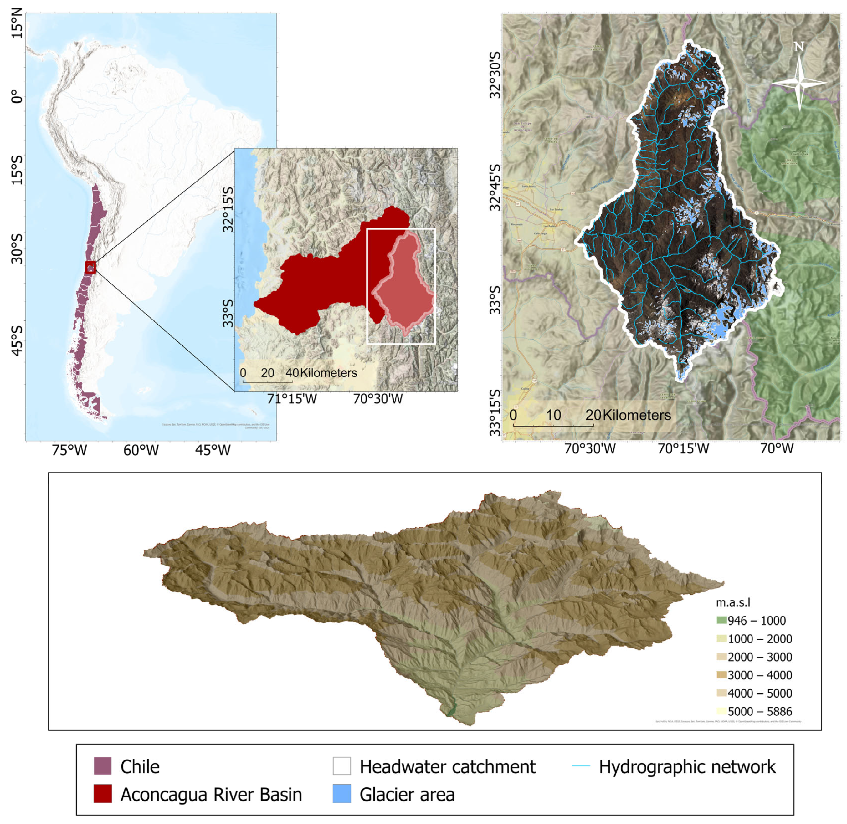
The headwater catchment of the Aconcagua River Basin is located in the Valparaíso Region, the second most populated region of Chile [25], between 32° and 33° latitude (Figure 1). It is a sub-basin of the Aconcagua River with three main tributaries (Juncal, Blanco and Colorado rivers), characterized as one of the main agricultural valleys in the country, relying mainly on water resources from snow and glaciers [26]. This headwater catchment covers approximately 28.84% of the total area of the basin and presents the highest altitude range, from 946 to 5886 m.a.s.l. The predominant hydrological regime is nival with an alpine climate characterized by low temperatures and solid precipitation, which favors snow accumulation and the presence of permanent ice fields [27]. According to the Public Glacier Inventory, ice bodies cover about 578 km², equivalent to 27.3% of the total surface area [28]. In addition, the basin also contains two protected areas: Juncal Andean Park and Río Blanco National Reserve [29].

3. Data

3.1. Remote Sensing Data

3.1.1. Optical Data

Snow cover analysis was processed using Landsat and the Moderate Resolution Imaging Spectroradiometer (MODIS) snow products. In the case of Landsat data, the Level-2 surface reflectance was used by applying atmospheric and topographic corrections, and cloud masking [30]. The Landsat data consists of imagery from Landsat 5, 7, 8, and 9 missions. These satellites provide 30 m spatial resolution and a 16-day revisit time. The combined use of these four missions enables the construction of an extensive time series of observations for the study area, with data available from 1985 to the present. On the other hand, the MODIS MOD10A1 (Terra) and MYD10A1 (Aqua) snow products were incorporated, providing snow cover data through a mapping approach based on the Normalized Difference Snow Index (NDSI) [31]. This product provides daily snow information at 500 m spatial resolution. The high temporal frequency allows a continuous database since the year 2002 for the basin; however, its relatively low spatial resolution makes it necessary to complement it with data from other satellites. Finally, surface albedo data were also obtained from the MODIS Snow Cover Daily Global 500 m products (Terra: MOD10A1; Aqua: MYD10A1).

3.1.2. Climatic Data

ERA5 is the latest fifth-generation global atmospheric reanalysis developed by the European Center for Medium-Range Weather Forecasts (ECMWF). The reanalysis period goes from 1950 to the present, and it replaces the ERA-Interim reanalysis, which only covered the period from 1979 onwards. Compared to its predecessor, ERA-5 offers substantially higher spatial resolution (31 km) and hourly temporal resolution, providing a more detailed representation of atmospheric and surface processes [32]. However, in complex mountainous areas, the spatial resolution of ERA5 limits the capture of fine-scale variability and topographic effects, which can result in uncertainties in the representation of atmospheric variables [33]. The dataset included: Air temperature, relative humidity, and snowfall. These data were used to complement in situ measurements and satellite observations in the analysis of snow cover dynamics.

4. Methodology

4.1. Preprocessing

Imagery was filtered to include all images covering the basin. A cloud mask with a maximum cloud cover threshold of 40% was applied to all image collections to ensure that cloud presence did not interfere with snow detection. For MODIS imagery, the Cloud Removal Algorithm for Snow-Covered Areas described by Mattar et al. [34] was used. Moreover, for Landsat imagery, the Quality Assessment (QA) bands were used to identify and mask clouds. In the case of Landsat 7, the Scan Line Corrector (SLC)-off gap filling correction was performed using a multi-scale focal mean interpolation approach. Gaps in Landsat 7 imagery can represent an important loss of information and potentially affect snow-covered area (SCA) estimation [35]. ERA5 reanalysis variables were also processed. This included converting 2 m air temperature from Kelvin to degrees Celsius and calculating relative humidity from air temperature and dew point temperature.

4.2. Snow Cover Classification

Snow cover classification was performed using the Normalized Difference Snow Index (NDSI), which uses the contrast between the high reflectance of snow in the green band of the visible spectrum and its low reflectance in the short-wave infrared. A threshold of NDSI ≥ 0.4 was applied: pixels with values equal to or above this threshold were classified as snow, while those below were considered snow-free [36]. In mountainous areas, different NDSI thresholds have been shown to be effective for snow detection; for example, Keshri et al. [37] reported satisfactory results using a threshold of 0.6. In Chile, however, a threshold of 0.4 has been widely applied, showing consistent and reliable results, as reported in previous studies [18,19,24].

The equation of the NDSI is:

$$NDSI={\displaystyle \frac{{\rho }_{Green}- {\rho }_{Swir}}{{\rho }_{Green}+{\rho }_{Swir}}}$$

(1)

where ρ_Green corresponds to the reflectance in the green band and ρ_SWIR to the reflectance in the short-wave infrared band.

4.3. Trend Analysis

The Mann–Kendall (MK) test was used to assess the presence of significant trends in the time series. This non-parametric test is frequently used for trend detection in meteorological data [38]. The MK test presents a null hypothesis (H₀), which assumes that there is no trend in the data series and that the data are identically distributed. The alternative hypothesis (H₁) assumes that there is a monotonic trend. The MK statistic S is given by:

$$S={\displaystyle \sum _{i=1}^{n-1}}{\displaystyle \sum _{j=i+1}^n}sign(x_j-x_i)$$

(2)

A positive value of S indicates an increasing trend, while a negative value indicates a decreasing trend. The function sign(x) indicates the direction of the difference between two observations, and is defined as:

$$sign\left(x\right)=\{\begin{array}{r}+1, x>0\\ 0, x=0\\ -1, x<0\end{array}$$

(3)

When the sample size is greater than 10, statistic S is assumed to follow a normal distribution, and its variance is computed as:

$$Var\left(S\right)={\displaystyle \frac{1}{18}}\left[n\left(n-1\right)\left(2n+5\right)-{\displaystyle \sum _{q=1}^g}{t}_q(t_q-1)(2t_q+5)\right]$$

(4)

The standardized test statistics Z is calculated as follows:

$$Z=\{\begin{array}{r}{\displaystyle \frac{S-1}{\sqrt{Var\left(S\right)}}}, S>0\\ 0, S=0\\ {\displaystyle \frac{S+1}{\sqrt{Var\left(S\right)}}}, S<0\end{array}$$

(5)

The MK test was computed for all variables, including snow-covered area (SCA), ERA5 variables, and albedo, using a significance level of 0.05. For monthly variables, the Seasonal Mann–Kendall test was applied in order to account for seasonal variability in the time series. This evaluates trends within each individual month separately, avoiding comparisons between months with different climatological conditions [39]. If a significant trend was detected using the Mann–Kendall test, its magnitude was estimated using the non-parametric Sen’s slope estimator, which is robust to outliers. Sen’s slope ($Q_{ij}$) was obtained as the median slope derived from all observation pairs. Equation (6):

$$Q_{ij}={\displaystyle \frac{x_j-x_i}{t_j-t_i}}$$

(6)

where $x_i$ and $x_j$ are observations at times $t_i$ and $t_j$ respectively (with $j$ > $i$).

To assess the temporal variability of all datasets, monthly and seasonal anomalies were calculated as the difference between the observed value for each month/season and the corresponding monthly or seasonal mean. Equation (7):

$$ai=x_i-\overline{x}$$

(7)

where x_i is the observed value for a given month/season and $\overline{x}$ is the corresponding mean of the time series.

Percent changes in SCA were then calculated by determining a baseline using the previous period to 2010 in order to determine the changes during the last decades (Equation (8)).

$$△\%={\displaystyle \frac{{SCA}_t-{SCA}_{baseline}}{{SCA}_{baseline}}}\ast 100$$

(8)

where SCA_t is the monthly SCA, and SCA_baseline corresponds to the mean monthly SCA during the baseline period.

5. Results and Analysis

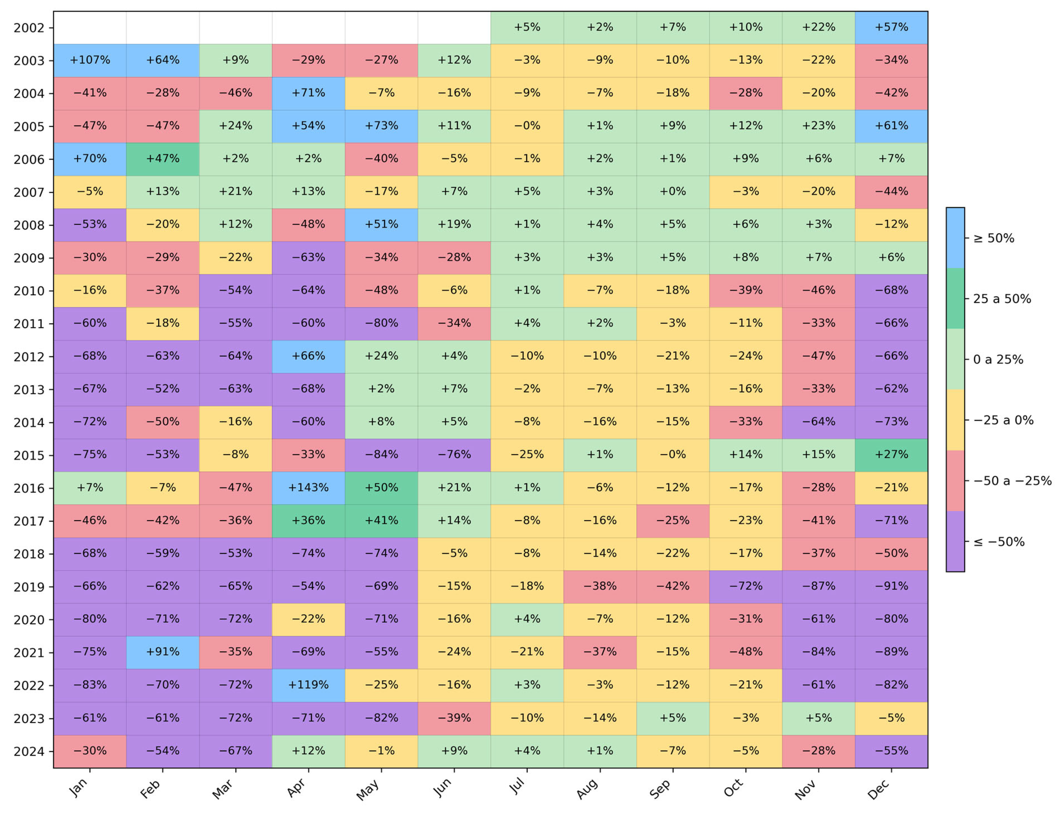
Figure 2 shows negative values of SCA after 2010 exceeding −50% in most years relative to the 2002–2009 baseline period. This period was selected as the reference baseline because it represents conditions prior to the onset of the central Chile megadrought in 2010 [40]. Declines are mainly observed during the late spring and summer (November to March), indicating reduced snow persistence and accelerated melting conditions. During winter (June to August), a more consistent variation of ±30% is observed, except for June 2015, which exhibits a decrease of 76% compared to the baseline. In addition, before 2010, April presented both positive and negative values, but after 2010, it presents mostly negative values, which indicates a variability in the onset of the snow season. Furthermore, the decrease in SCA during the years 2019–2021 presents the highest declines during the study period, with several months reaching reductions of almost 90% relative to the pre-drought period.

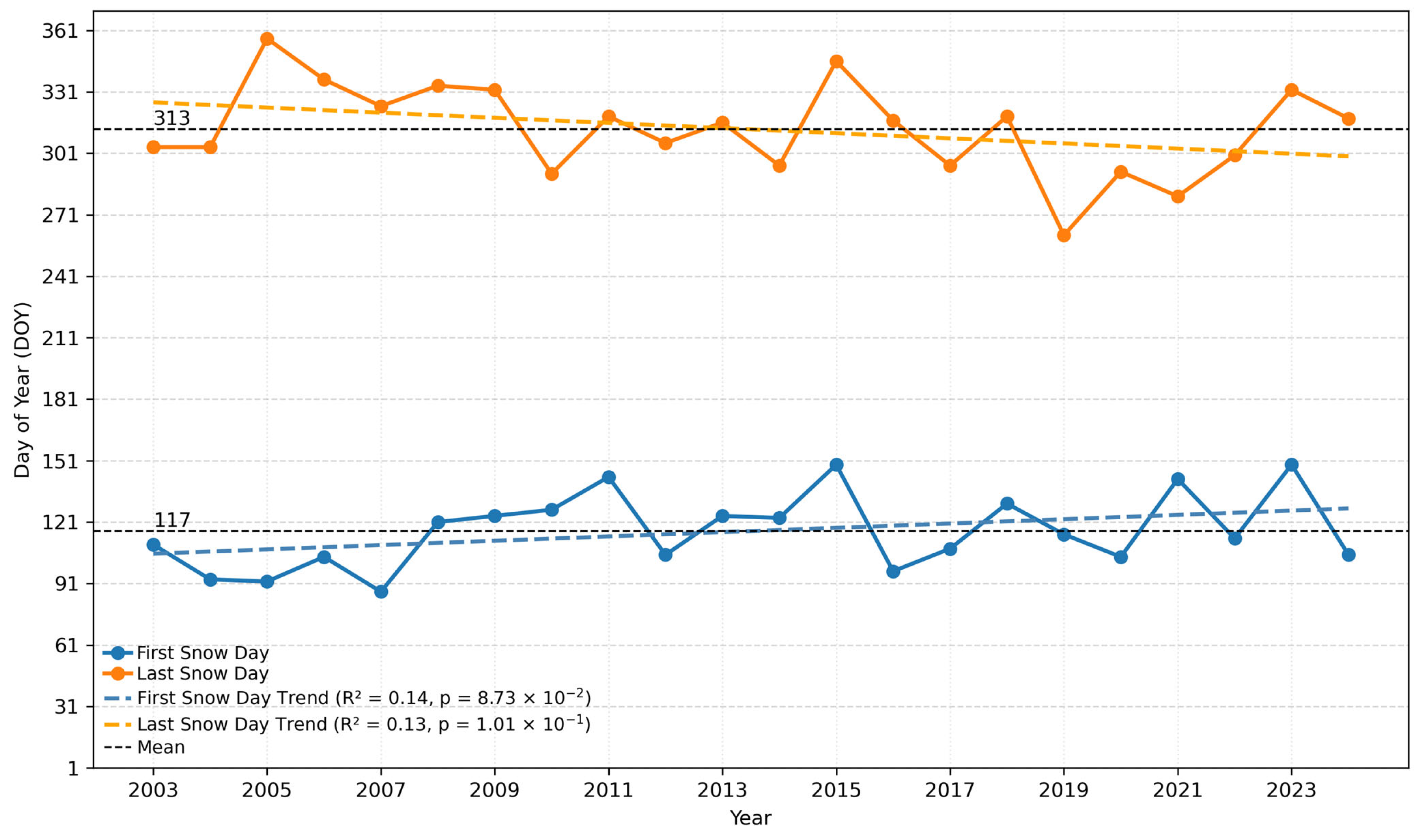
Figure 3 shows that the mean of the First Snow Day (FSD) and Last Snow Day (LSD) occur at approximately Day of Year (DOY) 117 and 313, respectively, resulting in a mean snow season duration of 196 days. The trends in FSD and LSD indicate a decrease in the duration of the snow season, characterized by a delayed onset and an earlier end. Specifically, based on the trend lines, the onset of the snow season shifted from DOY 105 in 2003 to DOY 127 in 2024, representing a delay of approximately 22 days. Similarly, the end of the snow season shifted from DOY 325 to DOY 299 over the same period, indicating an earlier end of about 26 days. Overall, these changes result in a shortening of the snow season of approximately 48 days.

5.1. Snow-Cover Trends: Landsat and MODIS

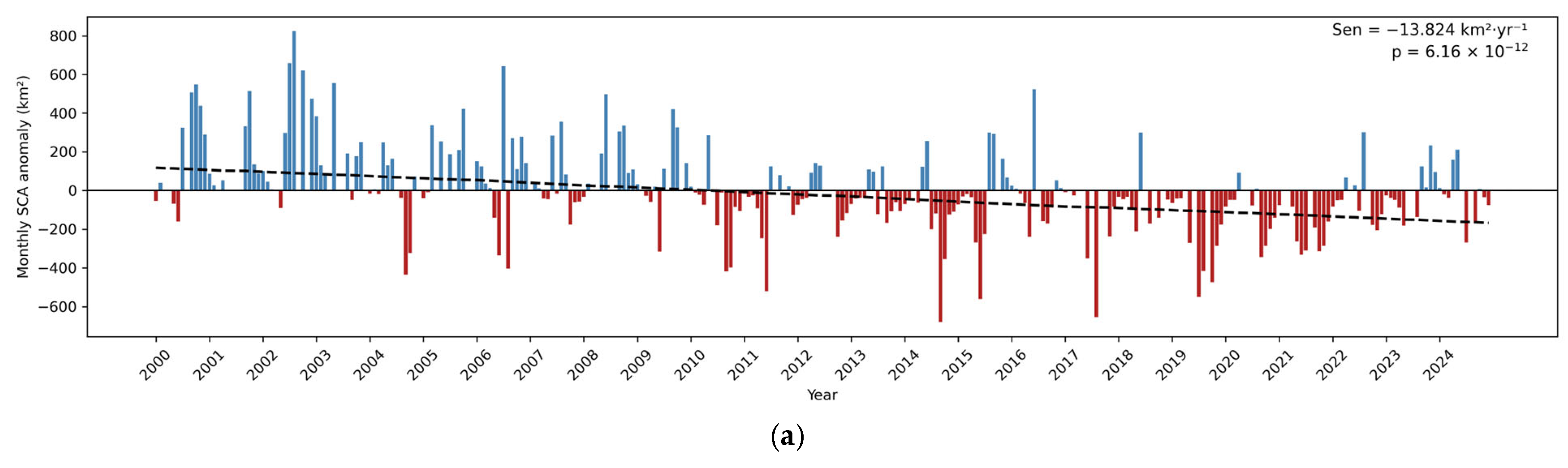
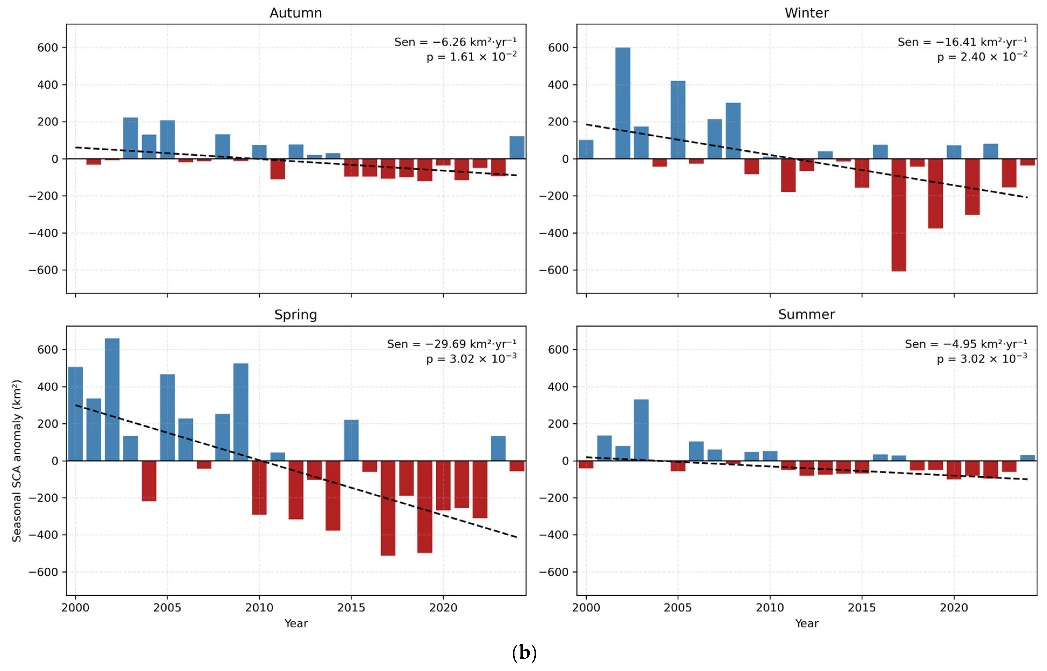
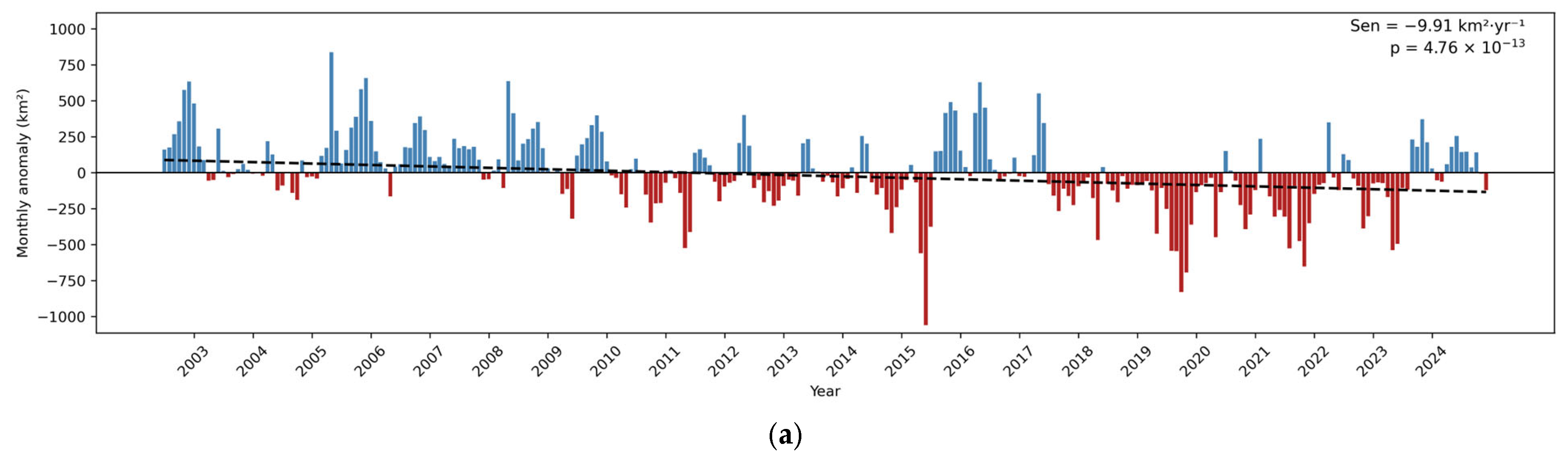
Monthly mean anomalies of SCA (Figure 4a) present predominant positive anomalies between 2000 and 2010 and mainly negative during 2010 to 2024, with a decrease of approximately 138.2 km² per decade. These trends are attributed to the megadrought, which might affect the snowfall and consequently the SCA. In addition, large-scale climate modes, particularly the positive phase of the Southern Annular Mode (SAM), have contributed to precipitation deficits, enhancing megadrought conditions and further reducing SCA [41]. For instance, Cordero et al. [42] reported severe and consecutive snow cover deficits between 2018 and 2021 in the extratropical Andes, with particularly pronounced deficits in the Aconcagua basin in 2019. Dietz et al. [43] describe a continuous rise in the Snow Line Elevation (SLE) in the Aconcagua Basin, which has a direct impact on the decrease in SCA, a trend that is expected to continue according to their results.

Seasonal SCA anomalies present a decrease in SCA over all seasons, with positive anomalies generally observed before 2010. Since the appearance of the megadrought, a series of negative anomalies has been found, with a predominant decline over the spring season, which presents a decline of about 296.6 km² per decade. This indicates a major reduction in the snowpack during the melting season and its direct impact on summer water availability. A similar response is found in the winter season, with a reduction of about 164.1 km² per decade, indicating a reduction in snowpack accumulation. As for the rest of the seasons, they present a smaller, but still significant, decline in comparison.

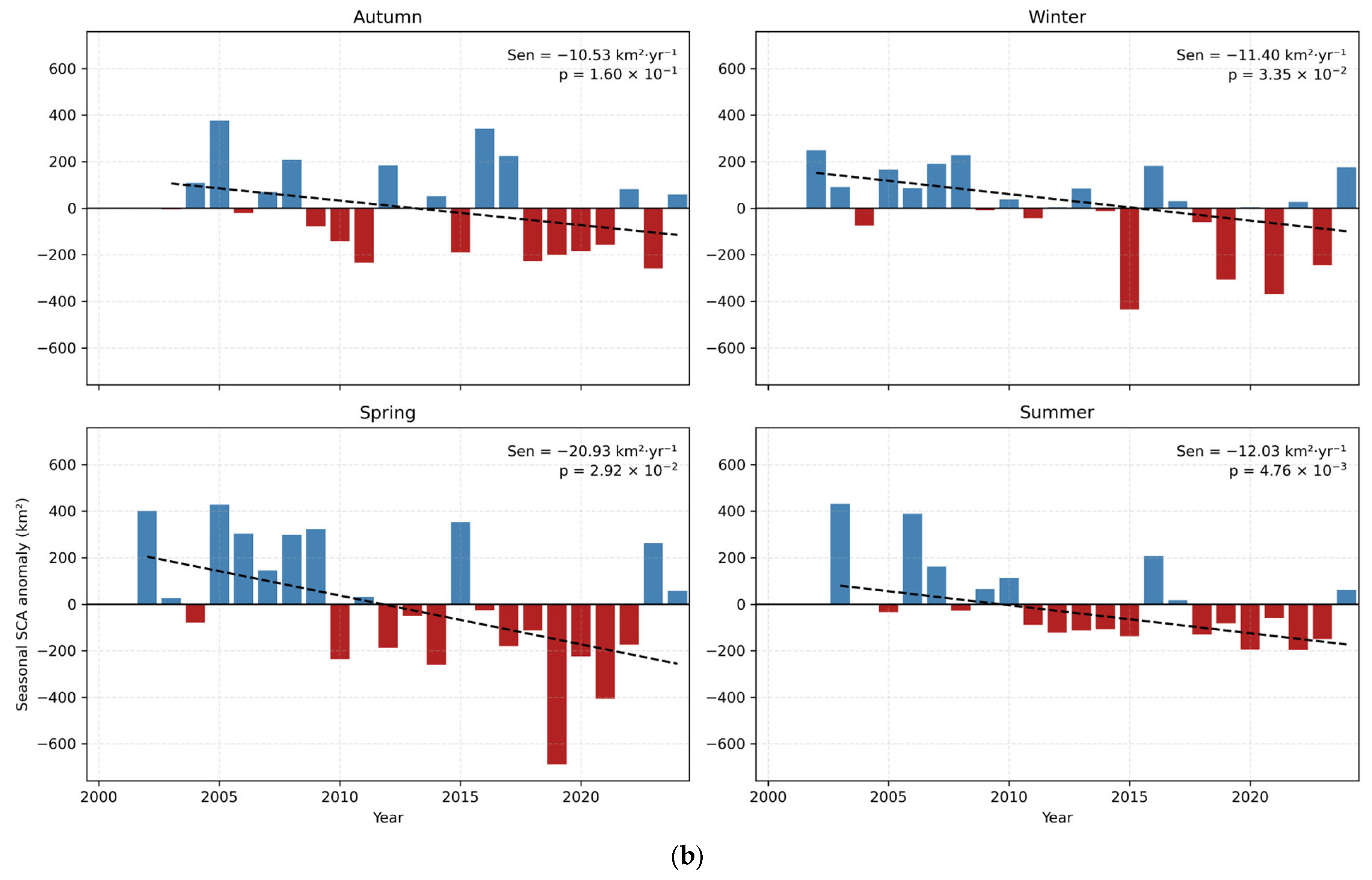
In the case of MODIS time series, anomalies show a similar behavior to Landsat data. This means a significant decreasing trend after 2010 (Figure 5a). The monthly anomalies indicate a decline of 9.91 km² per year, meaning that over the last two decades, there has been a reduction of 198.2 km² in SCA, equivalent to 9.3% of the basin area. These results are consistent with regional MODIS-based studies in the Central Andes, where approximately 80,000 km² of persistent snow cover loss between 29° S and 36° S has been reported [23]. Nevertheless, differences were observed between Landsat and MODIS trends in 2016 and 2017. While Landsat showed negative trends in those years, MODIS exhibited positive trends. This discrepancy might be explained by differences between the datasets, as MODIS provides a substantially larger number of observations than Landsat due to its daily temporal resolution. Nevertheless, both products show a continuous decline in SCA during the analyzed time period.

The available Landsat imagery used in this work represents approximately 26% (e.g., 2142 images) of the MODIS available snow product imagery between 2000 and 2024. Once the cloud threshold filter was applied, approximately 24% of the Landsat scenes were excluded from the analysis, resulting in 1626 Landsat images. Finally, less than 50% of the Landsat images cover the study area, resulting in a final Landsat dataset corresponding to 6% of the MODIS observations. Despite these differences, both datasets showed statistical consistency in the identified decreasing SCA trends, with an R² of 0.88 and a correlation coefficient of 0.90. These results indicate a temporal agreement between both datasets. However, due to the higher temporal resolution and larger number of available observations, the MODIS collection provided a more robust dataset for the time series analyses.

5.2. Snow Albedo

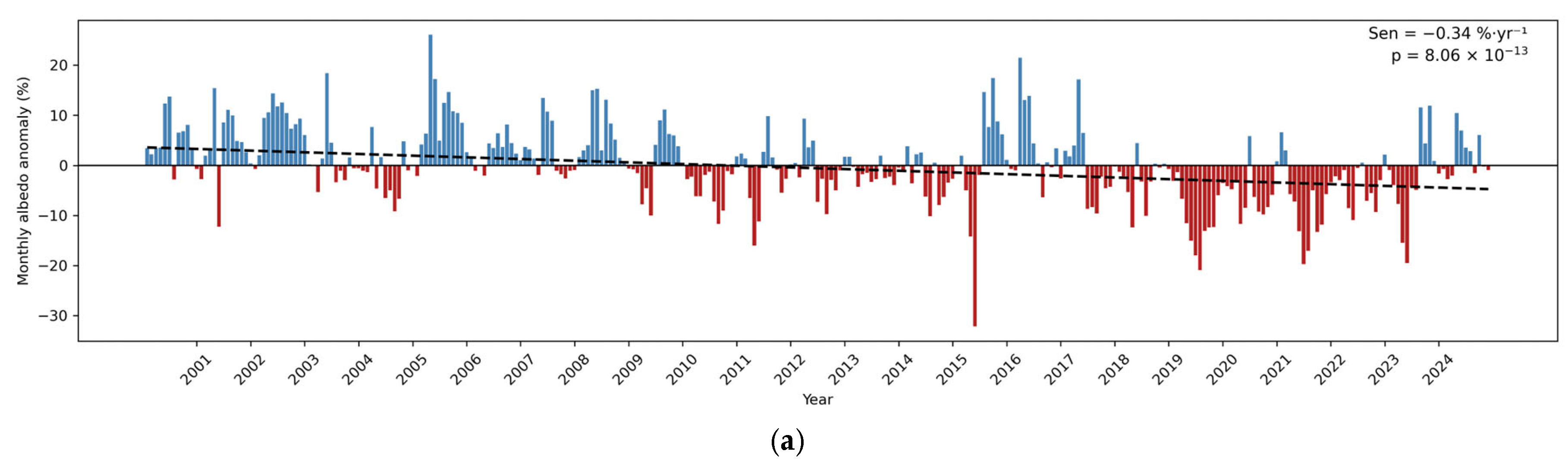
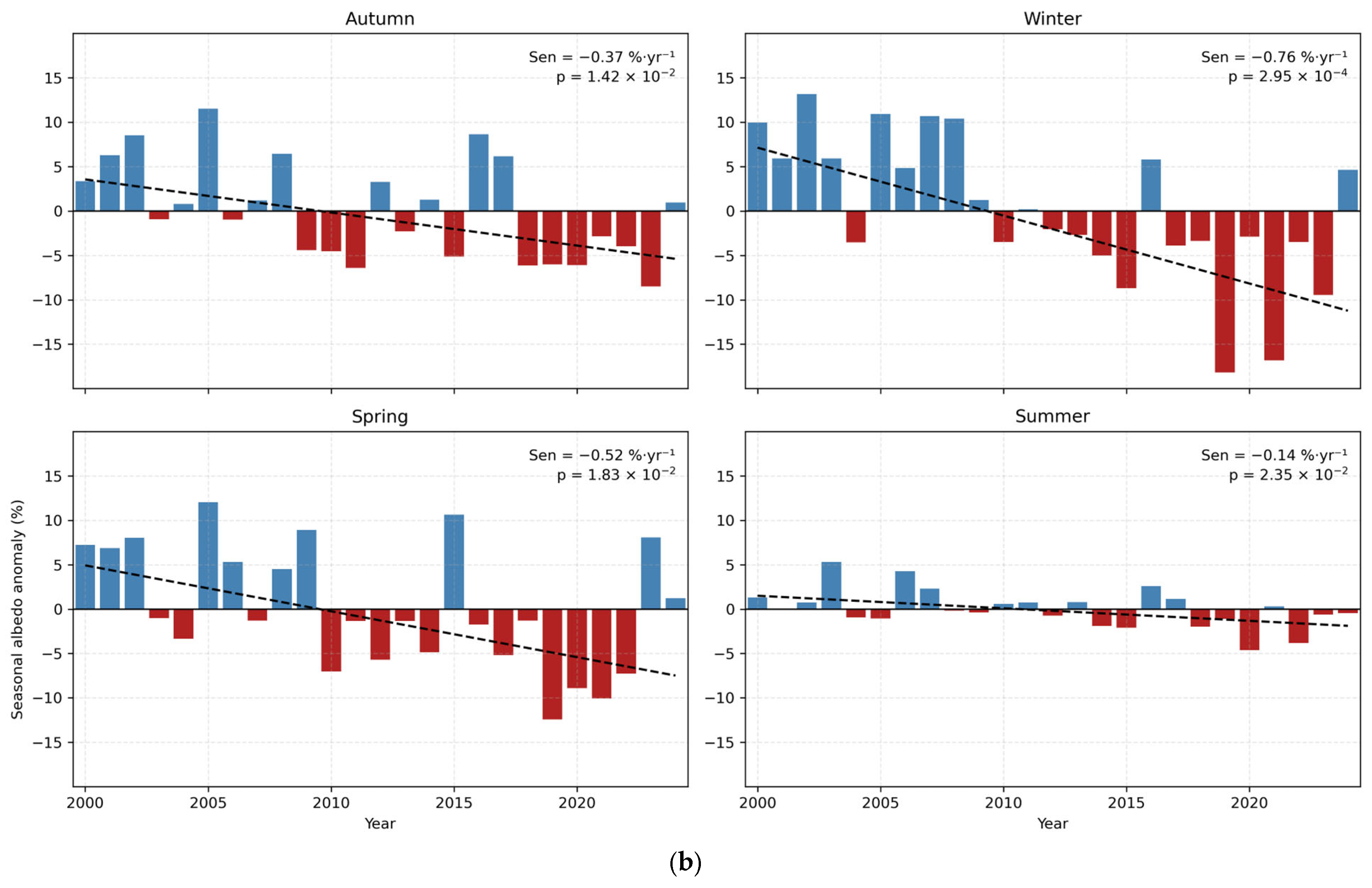
Figure 6a shows a significant decreasing trend in 4% per decade of snow albedo over the basin, with values below the mean after 2010. Although negative anomalies are mostly observed throughout the post-2010 period, the most noticeable declines are observed between 2015 and 2023. This decrease is consistent with the results of Figueroa-Villanueva et al. [44], who reported a decrease in snow albedo in the upper Aconcagua Basin over their study period (2004–2016). Ruggeri et al. [45] also reported increased black carbon concentrations associated with vehicular traffic in the Central Andes near the study area, potentially affecting snow albedo in the basin. Similar results were also documented in the Central Andes close to the study area [46]. Regarding seasonal anomalies, all seasons except summer show statistically significant decreasing trends, particularly winter and spring, which present the important reductions, −0.76% and −0.52% per year, respectively (Figure 6b).

5.3. Climate Trend Analysis

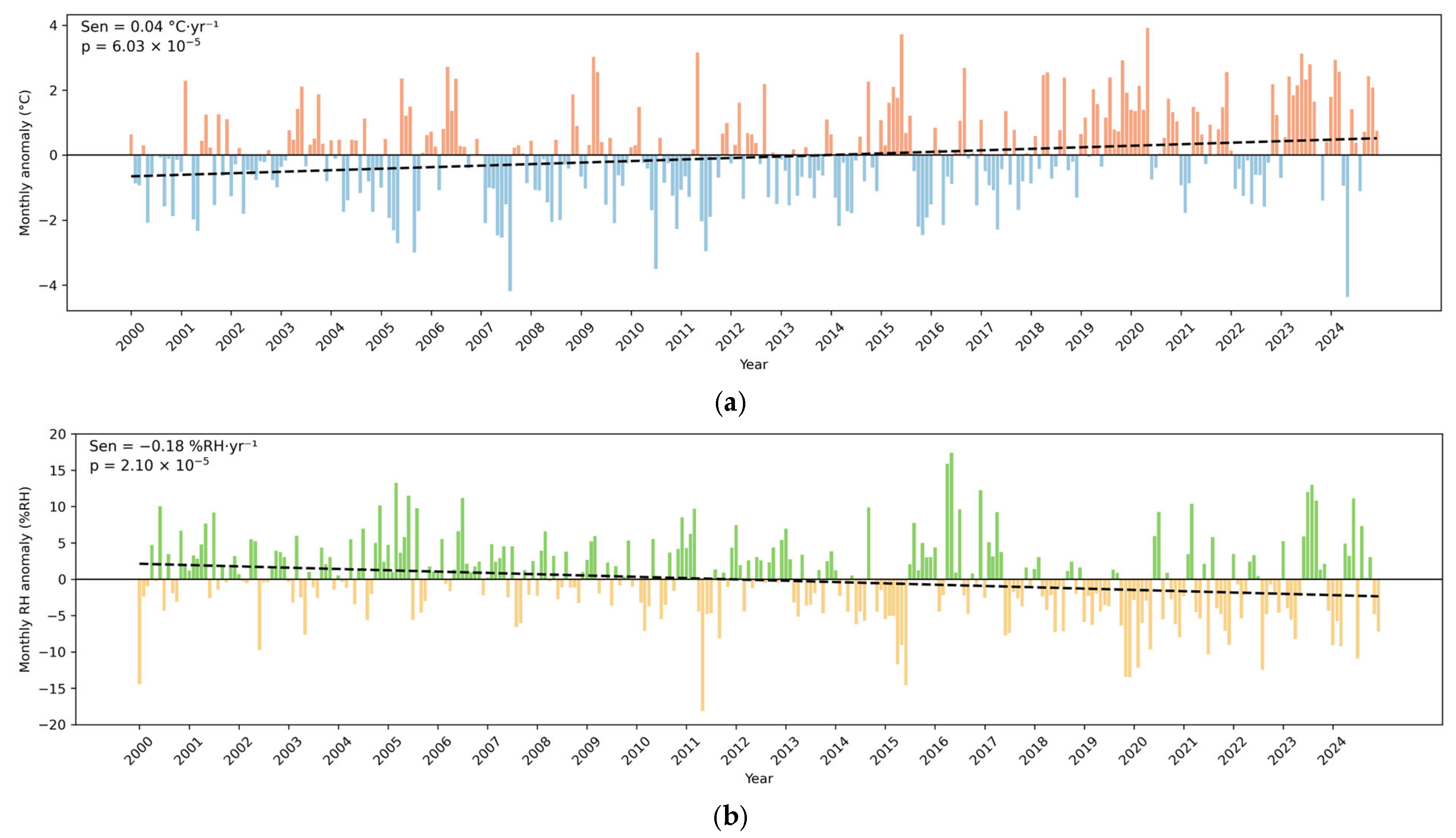
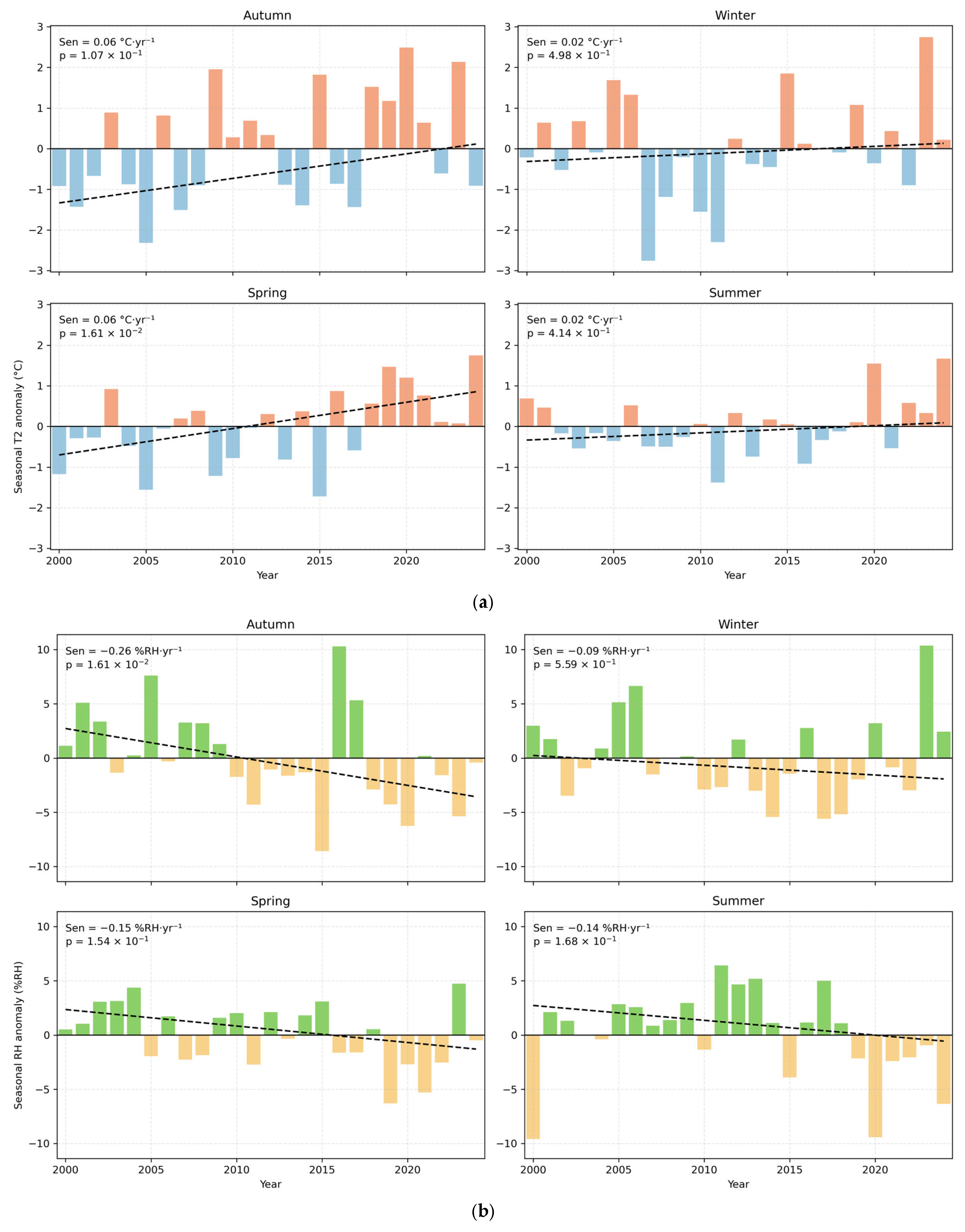
Figure 7a shows the air temperature (T2) monthly mean anomalies for the 2000–2024 period. A statistically significant warming trend is observed, indicating an approximate increase of 1 °C over the study period. The warmest anomalies are concentrated between 2015 and 2023, with several months exceeding +3 °C. In addition, all seasons exhibit a positive temperature trend; however, the only statistically significant warming is observed during spring (0.06 °C·yr⁻¹), indicating an accelerated warming during the melt season (Figure 8a). These results are consistent with the general increase in temperatures in mountainous regions, where the consequences of rising air temperatures are more intense at high altitudes, having direct impacts on snowfall rates due to snow responding faster to climate change than other elements of the cryosphere [47,48]. Furthermore, a negative correlation (r = −0.79) was observed between air temperature and SCA, suggesting that increasing temperatures are closely associated with reductions in snow cover. In central Chile, previous studies reported a sustained increase in air temperature and more frequent heatwaves. These trends impact not only SCA dynamics but also productive activities dependent on water availability in central Chile [22,23,24,25,26,27,28,29,30,31,32,33,34,35,36,37,38,39,40,41,42,43,44,45,46,47,48,49].

The relative humidity shows a decrease of about 1.8% per decade, with a statistically significant change point identified in 2013, marking the onset of a persistent decline (Figure 7b). This reduction is associated with the above-mentioned increase in air temperature, which shows a similar temporal pattern. The increase in air temperature and decrease in RH indicate progressively drier and warmer conditions, which might accelerate melt processes and shorten snow cover duration [50]. Seasonal RH anomalies change from predominantly positive values in the early 2000 s to mostly negative anomalies after 2010, indicating a transition toward progressively drier atmospheric conditions, with autumn being the only season showing a statistically significant trend (−0.26% per year) (Figure 8b).

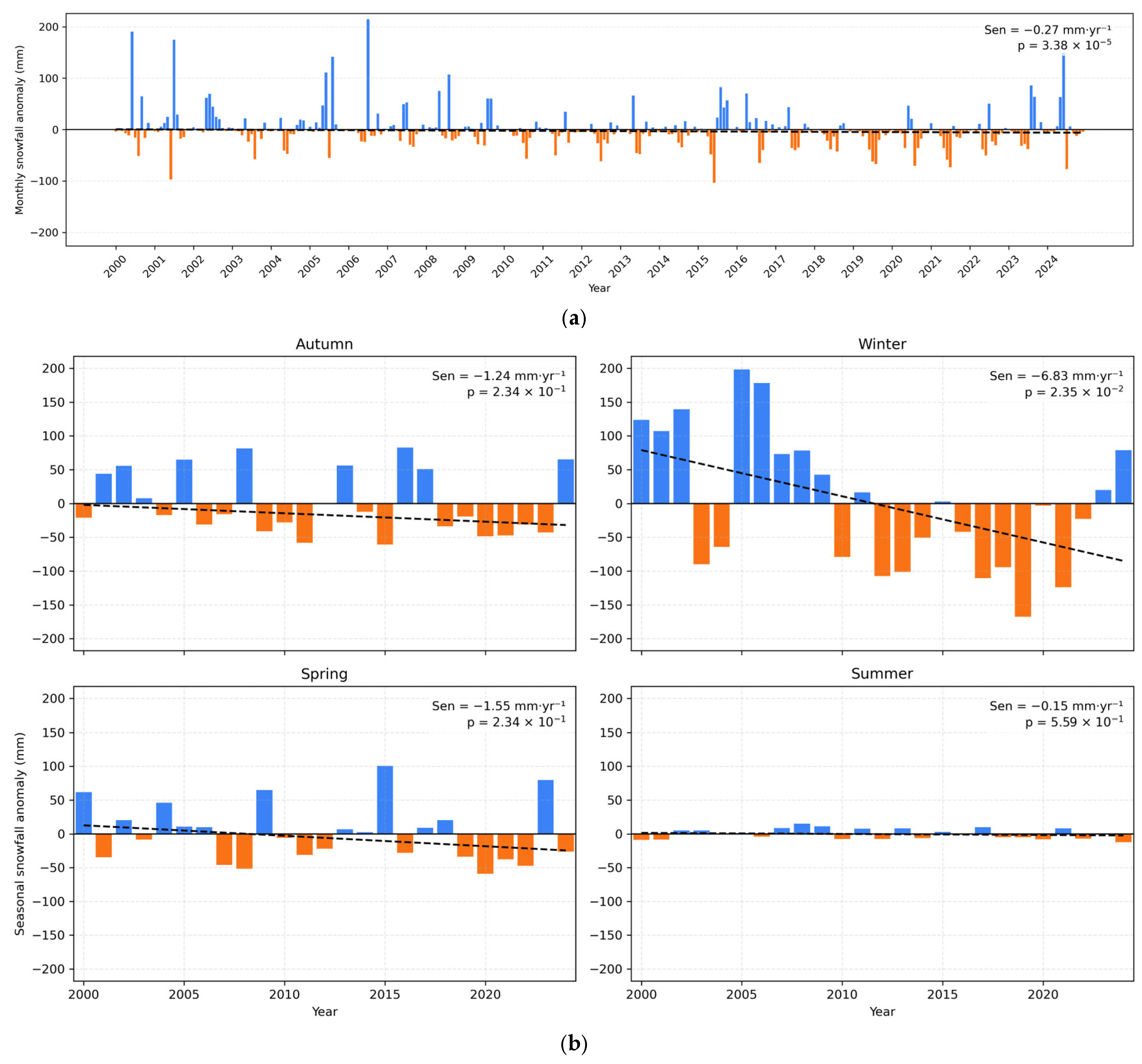
Snowfall shows a slight decrease over the study period, with an approximate decline of 2.7 mm per decade (Figure 9a). The main negative values were observed during the winter season, which presents predominantly negative values, where 2019 shows the greatest decline, reaching a reduction of over 150 mm (Figure 9b).

6. Discussion

Landsat and MODIS SCA trends show discrepancies that can be attributed to differences in temporal resolution and the number of available observations. Despite those facts, both datasets have shown decreasing trends in SCA similar to 13.8 km² per year and 9.91 km² per year, for Landsat and MODIS, respectively. The results showed a decrease in SCA during the last decades. At the seasonal temporal scale, SCA also showed decreasing trends, which indicates that the main changes occurred during the melting seasons, rather than being driven by reduced snow accumulation in winter. Nevertheless, the start and end of the phenological phase and its trends for the headwater catchment are still unknown owing to the lack of daily data and the cloudy days. To address this issue, it is necessary to reinforce the in situ snow network in order to obtain several snow parameters such as density, depth, snowfall, snow water equivalent (SWE), snow temperature, among others. In addition, other approaches are related to integrating simple and replicable monitoring technologies such as RGB cameras, which are key to improving snow monitoring in mountainous and inaccessible regions, as this method allows the acquisition of snow depth data for the estimation of SWE [51].

In the case of ERA-5, temperature and relative humidity demonstrate a significant warming trend and a decrease in humidity. Even though spatial resolution might affect the magnitude of the trends, both datasets demonstrate an impact on warming and the megadrought previously documented. This warming affects the snow cover and snow duration, which could be explained by the rising temperatures reported in this study. Increasing temperatures and recent heatwaves can accelerate snowmelt and reduce snow persistence, particularly during spring and summer [8]. These changes could also be enhanced by variations in snowpack properties, such as an increased liquid water content, deposition of light-absorbing particles such as black carbon, and reduced albedo. These could accelerate the melting season and shorten snow persistence. Several works have documented the impacts of warming trends in highland and mountain areas on the snow cover area and duration [44,45,46,47,48,49,50,51,52].

Atmospheric and climatic events could also affect the trends. A predominantly positive trend of SAM has been observed in central Chile. A positive SAM index is associated with the intensification and poleward migration of the westerly winds. Cordero et al. [42] and Garreaud et al. [41] indicate that precipitation losses in recent decades are partially attributed to this positive SAM trend, thereby affecting SCA. In addition, interannual variability associated with ENSO can also influence these trends. El Niño events that occurred (2002, 2004–2005, 2006–2007, 2009, 2015–2016, and 2023–2024) are generally associated with increased precipitation in central Chile, which can lead to an increase in snow-covered area at higher elevations [53]. This can be observed in Figure 2, where the years showing predominantly positive values during the spring and summer months correspond to El Niño phases. In contrast, persistent negative anomalies dominate after 2010, with extreme deficits during 2018–2021, consistent with the prolonged dry conditions in central Chile and overlapping with La Niña phases (e.g., 2010–2011 and 2020–2022) [54].

7. Conclusions

The SCA over the headwater catchment of the Aconcagua basin was analyzed using satellite remote sensing data and compared with climatic data. Local warming trends were identified based on the reanalysis dataset, with a persistent decline in SCA. These changes might have a considerable impact on water reservoirs in the basin and water availability, since this headwater catchment is key for water supply due to snow accumulation and glacier presence. The results reported in this study are consistent with previous research in the basin and highlight the need to increase in situ measurements through the installation of additional ground stations, including SWE measurements, one of the most sensitive indicators of climate change impacts. Future efforts should aim to analyze the relation between snow cover and streamflow to better understand the availability of water resources and demand. This would improve the understanding of the current and future status of the basin and support sustainable water management.

References

1. He, B.; Chang, J.; Guo, A.; Wang, L.; Li, Z.; Zhai, D.; Gao, F. Spatial and temporal runoff variability in response to climate change in alpine mountains. J. Hydrol. 2025, 654, 132779. [Google Scholar] [CrossRef]
2. Hock, R.; Rasul, G.; Adler, C.; Cáceres, B.; Gruber, S.; Hirabayashi, Y.; Jackson, M.; Kääb, A.; Kang, S.; Kutuzov, S.; et al. High Mountain Areas. In IPCC Special Report on the Ocean and Cryosphere in a Changing Climate; Pörtner, H.-O., Roberts, D.C., Masson-Delmotte, V., Zhai, P., Tignor, M., Poloczanska, E., Mintenbeck, K., Alegría, A., Nicolai, M., Okem, A., et al., Eds.; IPCC: Geneva, Switzerland, 2019; Available online: https://iris.unito.it/bitstream/2318/1803038/1/06_SROCC_Ch02_FINAL.pdf (accessed on 20 September 2025).
3. Xiao, X.; Zhang, T.; Zhong, X.; Li, X. Spatiotemporal variation of snow depth in the Northern Hemisphere from 1992 to 2016. Remote Sens. 2020, 12, 2728. [Google Scholar] [CrossRef]
4. Notarnicola, C. Overall negative trends for snow cover extent and duration in global mountain regions over 1982–2020. Sci. Rep. 2022, 12, 13731. [Google Scholar] [CrossRef] [PubMed]
5. Tang, Z.; Deng, G.; Hu, G.; Zhang, H.; Pan, H.; Sang, G. Satellite observed spatiotemporal variability of snow cover and snow phenology over High Mountain Asia from 2002 to 2021. J. Hydrol. 2022, 613, 128438. [Google Scholar] [CrossRef]
6. Adler, C.; Wester, P.; Bhatt, I.; Huggel, C.; Insarov, G.E.; Morecroft, M.D.; Muccione, V.; Prakash, A. Cross-Chapter Paper 5: Mountains. In Climate Change 2022: Impacts, Adaptation and Vulnerability. Contribution of Working Group II to the Sixth Assessment Report of the Intergovernmental Panel on Climate Change; Pörtner, H.-O., Roberts, D.C., Tignor, M., Poloczanska, E.S., Mintenbeck, K., Alegría, A., Craig, M., Langsdorf, S., Löschke, S., Möller, V., et al., Eds.; Cambridge University Press: Cambridge, UK; New York, NY, USA, 2022; pp. 2273–2318. [Google Scholar] [CrossRef]
7. Immerzeel, W.W.; Lutz, A.F.; Andrade, M.; Bahl, A.; Biemans, H.; Bolch, T.; Hyde, S.; Brumby, S.; Davies, B.J.; Elmore, A.C.; et al. Importance and vulnerability of the world’s water towers. Nature 2020, 577, 364–369. [Google Scholar] [CrossRef]
8. Poveda, G.; Espinoza, J.C.; Zuluaga, M.D.; Solman, S.A.; Garreaud, R.; Van Oevelen, P.J. High impact weather events in the Andes. Front. Earth Sci. 2020, 8, 162. [Google Scholar] [CrossRef]
9. Pérez, T.; Mattar, C.; Fuster, R. Decrease in Snow Cover over the Aysén River Catchment in Patagonia, Chile. Water 2018, 10, 619. [Google Scholar] [CrossRef]
10. Olivares-Contreras, V.A.; Mattar, C.; Gutiérrez, A.G.; Jiménez, J.C. Warming trends in Patagonian subantartic forest. Int. J. Appl. Earth Obs. Geoinf. 2019, 76, 51–65. [Google Scholar] [CrossRef]
11. Olivera-Guerra, L.; Quintanilla, M.; Moletto-Lobos, I.; Pichuante, E.; Zamorano-Elgueta, C.; Mattar, C. Water dynamics over a Western Patagonian watershed: Land surface changes and human factors. Sci. Total Environ. 2022, 804, 150221. [Google Scholar] [CrossRef]
12. Dirección General de Aguas (DGA). Redefinición de la Clasificación de la Red Hidrográfica a Nivel Nacional; Informe Técnico S.D.T. Nº 356; Ministerio de Obras Públicas, Gobierno de Chile: Santiago, Chile, 2014.
13. Jara, F.; Lagos-Zúñiga, M.; Fuster, R.; Mattar, C.; McPhee, J. Snow processes and climate sensitivity in an Arid Mountain Region, Northern Chile. Atmosphere 2021, 12, 520. [Google Scholar] [CrossRef]
14. Saavedra, F.A.; Kampf, S.K.; Fassnacht, S.R.; Sibold, J.S. Changes in Andes snow cover from MODIS data, 2000–2016. Cryosphere 2018, 12, 1027–1046. [Google Scholar] [CrossRef]
15. Dussaillant, I.; Berthier, E.; Brun, F.; Masiokas, M.; Hugonnet, R.; Favier, V.; Rabatel, A.; Pitte, P.; Ruiz, L. Two decades of glacier mass loss along the Andes. Nat. Geosci. 2019, 12, 802–808. [Google Scholar] [CrossRef]
16. Dirección General de Aguas (DGA). Base de Datos de la Red Hidrométrica Nacional: Reportes Estadísticos de Variables Hidrometeorológicas y Calidad de Aguas (Database); Ministerio de Obras Públicas (MOP): Santiago, Chile, 2025. Available online: https://dga.mop.gob.cl/estadisticas-estaciones-dga/ (accessed on 26 September 2025).
17. Condom, T.; Martínez, R.; Pabón, J.D.; Costa, F.; Pineda, L.; Nieto, J.J.; Lopéz, F.; Villacis, M. Climatological and hydrological observations for the South American Andes: In situ stations, satellite, and reanalysis data sets. Front. Earth Sci. 2020, 8, 92. [Google Scholar] [CrossRef]
18. Aranda, F.; Medina, D.; Castro, L.; Ossandón, Á.; Ovalle, R.; Flores, R.P.; Bolaño-Ortiz, T.R. Snow persistence and snow line elevation trends in a Snowmelt-Driven Basin in the Central Andes and their correlations with hydroclimatic variables. Remote Sens. 2023, 15, 5556. [Google Scholar] [CrossRef]
19. Masiokas, M.H.; Rabatel, A.; Rivera, A.; Ruiz, L.; Pitte, P.; Ceballos, J.L.; Barcaza, G.; Soruco, A.; Brown, E.; Dussaillant, I.; et al. A review of the current state and recent changes of the Andean cryosphere. Front. Earth Sci. 2020, 8, 99. [Google Scholar] [CrossRef]
20. MacFee, M.; Carrivick, J.L.; Quincey, D.J. Rising snowline altitudes across Southern Hemisphere glaciers from 2000 to 2023. Sci. Rep. 2025, 15, 35683. [Google Scholar] [CrossRef] [PubMed]
21. Ministerio del Medio Ambiente (MMA). Informe Técnico de la Elaboración del Proyecto Definitivo de las Normas Secundarias de Calidad Ambiental Para la Protección de las Aguas Continentales Superficiales de la Cuenca del río Aconcagua; División de Recursos Naturales y Biodiversidad, Departamento de Ecosistemas Acuáticos, SEREMI del Medio Ambiente Región de Valparaíso: Valparaíso, Chile, 2021. [Google Scholar]
22. Webb, M.J.; Winter, J.M.; Spera, S.A.; Chipman, J.W.; Osterberg, E.C. Water, agriculture, and climate dynamics in central Chile’s Aconcagua River Basin. Phys. Geogr. 2021, 42, 395–415. [Google Scholar] [CrossRef]
23. Saavedra, F.; Hernández-Duarte, A.; Caro, A.; Rabatel, A.; Fassnacht, S.; Condom, T.; Kampf, S.; Masiokas, M.; Romero, C.; Aguirre, Y.; et al. Spatial and temporal variability of snow in the Andes using MODIS snow product 2000–2025. Front. Earth Sci. 2026, 14, 1564035. [Google Scholar] [CrossRef]
24. Cordero, R.R.; Asencio, V.; Feron, S.; Damiani, A.; Llanillo, P.J.; Sepulveda, E.; Jorquera, J.; Carrasco, J.; Casassa, G. Dry-Season Snow Cover Losses in the Andes (18°–40°S) driven by Changes in Large-Scale Climate Modes. Sci. Rep. 2019, 9, 16945. [Google Scholar] [CrossRef]
25. Instituto Nacional de Estadísticas (INE) de Chile. Resultados Censo 2024—Dashboard. Available online: https://censo2024.ine.gob.cl/resultados-dashboard/ (accessed on 30 September 2025).
26. Janke, J.R.; Ng, S.; Bellisario, A. An inventory and estimate of water stored in firn fields, glaciers, debris-covered glaciers, and rock glaciers in the Aconcagua River Basin, Chile. Geomorphology 2017, 296, 142–152. [Google Scholar] [CrossRef]
27. Centro de Información de Recursos Naturales (CIREN). Recursos Naturales: Comuna de Los Andes; SIT Rural (Sistema de Información Territorial); CIREN: Santiago, Chile, 2023. [Google Scholar]
28. Dirección General de Aguas (DGA); Ministerio de Obras Públicas (MOP). Inventario Público de Glaciares 2022 (Dataset); Gobierno de Chile: Santiago, Chile, 2022. Available online: https://dga.mop.gob.cl/uploads/sites/13/2025/05/Glaciares.zip (accessed on 26 September 2025).
29. Escenarios Hídricos 2030. Transición Hídrica: El Futuro del Agua en Chile; Fundación Chile: Santiago, Chile, 2019; Volume 1, Available online: https://escenarioshidricos.cl/wp-content/uploads/2021/06/Transicion-hidrica-el-futuro-del-agua-en-Chile-v.1_compressed.pdf (accessed on 2 October 2025).
30. Zhou, Y.; Jiang, H.; Wang, Z.; Yang, X.; Geng, E. Assessment of four typical topographic corrections in Landsat TM data for snow cover areas. Int. Arch. Photogramm. Remote Sens. Spat. Inf. Sci. 2016, 41, 157–162. [Google Scholar] [CrossRef]
31. Hall, D.K.; Riggs, G.A. Normalized-difference snow index (NDSI). In Encyclopedia of Snow, Ice and Glaciers; Singh, V.P., Singh, P., Haritashya, U.K., Eds.; Springer: Dordrecht, The Netherlands, 2011; pp. 779–780. [Google Scholar] [CrossRef]
32. Hersbach, H.; Bell, B.; Berrisford, P.; Hirahara, S.; Horányi, A.; Muñoz-Sabater, J.; Nicolas, J.; Peubey, C.; Radu, R.; Schepers, D.; et al. The ERA5 global reanalysis. Q. J. R. Meteorol. Soc. 2020, 146, 1999–2049. [Google Scholar] [CrossRef]
33. Wang, J.; Li, Z.; Liang, Y.; Ke, J. An Assessment of the Applicability of ERA5 Reanalysis Boundary Layer Data Against Remote Sensing Observations in Mountainous Central China. Atmosphere 2025, 16, 1152. [Google Scholar] [CrossRef]
34. Mattar, C.; Fuster, R.; Perez, T. Application of a Cloud Removal Algorithm for Snow-Covered Areas from Daily MODIS Imagery over Andes Mountains. Atmosphere 2022, 13, 392. [Google Scholar] [CrossRef]
35. Chen, J.; Zhu, X.; Vogelmann, J.E.; Gao, F.; Jin, S. A simple and effective method for filling gaps in Landsat ETM+ SLC-off images. Remote Sens. Environ. 2011, 115, 1053–1064. [Google Scholar] [CrossRef]
36. Dozier, J. Spectral Signature of Alpine Snow Cover from the Landsat Thematic Mapper. Remote Sens. Environ. 1989, 28, 9–22. [Google Scholar] [CrossRef]
37. Keshri, A.K.; Shukla, A.; Gupta, R.P. ASTER ratio indices for supraglacial terrain mapping. Int. J. Remote Sens. 2009, 30, 519–524. [Google Scholar] [CrossRef]
38. Thapa, S.; Li, B.; Fu, D.; Shi, X.; Tang, B.; Qi, H.; Wang, K. Trend analysis of climatic variables and their relation to snow cover and water availability in the Central Himalayas: A case study of Langtang Basin, Nepal. Theor. Appl. Climatol. 2020, 140, 891–903. [Google Scholar] [CrossRef]
39. Hirsch, R.M.; Slack, J.R. A nonparametric trend test for seasonal data with serial dependence. Water Resour. Res. 1984, 20, 727–732. [Google Scholar] [CrossRef]
40. Kim, Y.; Kim, S.; Jeong, H.; An, H. Quantitatively defining megadrought based on drought events in central Chile. Geomat. Nat. Hazards Risk 2022, 13, 975–992. [Google Scholar] [CrossRef]
41. Garreaud, R.D.; Boisier, J.P.; Rondanelli, R.; Montecinos, A.; Sepúlveda, H.H.; Veloso-Aguila, D. The Central Chile Mega Drought (2010–2018): A climate dynamics perspective. Int. J. Climatol. 2020, 40, 421–439. [Google Scholar] [CrossRef]
42. Cordero, R.R.; Feron, S.; Damiani, A.; MacDonell, S.; Carrasco, J.; Pizarro, J.; Karas, C.; Jorquera, J.; Sepulveda, E.; Cabello, F.; et al. Rapid decline in extratropical Andean snow cover driven by the poleward migration of the Southern Hemisphere westerlies. Sci. Rep. 2024, 14, 26365. [Google Scholar] [CrossRef]
43. Dietz, A.J.; Köhler, J.; Obrecht, L.; Rößler, S.; Baumhoer, C.A.; Cereceda-Balic, F.; Saavedra, F. Snow Cover Trends in the Chilean Andes Derived from 39 Years of Landsat Data and a Projection for the Year 2050. Remote Sens. 2025, 17, 1651. [Google Scholar] [CrossRef]
44. Figueroa-Villanueva, L.; Castro, L.; Bolaño-Ortiz, T.R.; Flores, R.P.; Pacheco-Ferrada, D.; Cereceda-Balic, F. Changes in Snow Surface Albedo and Radiative Forcing in the Chilean Central Andes Measured by In Situ and Remote Sensing Data. Water 2023, 15, 3198. [Google Scholar] [CrossRef]
45. Ruggeri, M.F.; Bolaño-Ortiz, T.; Cereceda-Balic, F. Atmospheric black carbon in a key location of the Chilean Central Andes: Identifying patterns, sources, and potential impacts. Atmos. Environ. 2024, 318, 120273. [Google Scholar] [CrossRef]
46. Sánchez-López, R.; Mattar, C.; Bravo, C.; Durán-Alarcón, C.; Jenk, T.M. Monitoring of light absorbing impurities (LAIs) in snow and glaciers along the Central Andes. Recent Adv. Remote Sens. 2025, 2, 4. [Google Scholar] [CrossRef]
47. Wu, X.; Shen, Y.; Zhang, W.; Long, Y. Fast Warming Has Accelerated Snow Cover Loss during Spring and Summer across the Northern Hemisphere over the Past 52 Years (1967–2018). Atmosphere 2020, 11, 728. [Google Scholar] [CrossRef]
48. Bilbao Barrenetxea, N.; Faria, S.H. Climate change in high-mountain regions: An international perspective and a look at the Pyrenees. Métode Sci. Stud. J. 2022, 12, 115–121. [Google Scholar] [CrossRef]
49. González-Reyes, Á.; Jacques-Coper, M.; Bravo, C.; Rojas, M.; Garreaud, R. Evolution of heatwaves in Chile since 1980. Weather Clim. Extrem. 2023, 41, 100588. [Google Scholar] [CrossRef]
50. Zhen, S.; Zhang, Z.; Wang, X.; Zhao, H.; Yin, Y. Duration of the influence of snowmelt on land surface temperature and humidity after snowmelt on the Mongolian Plateau. Sci. Total Environ. 2023, 900, 166433. [Google Scholar] [CrossRef] [PubMed]
51. Tanis, C.M.; Lindgren, E.; Frey, A.; Latva, L.; Arslan, A.N.; Luojus, K. Use of Webcams in Support of Operational Snow Monitoring. Geosciences 2023, 13, 92. [Google Scholar] [CrossRef]
52. Koch, F.; Prasch, M.; Schmid, L.; Schweizer, J.; Mauser, W. Measuring Snow Liquid Water Content with Low-Cost GPS Receivers. Sensors 2014, 14, 20975–20999. [Google Scholar] [CrossRef]
53. Campos, D.; Rondanelli, R. ENSO-related precipitation variability in Central Chile: The role of large scale moisture transport. J. Geophys. Res. Atmos. 2023, 128, e2023JD038671. [Google Scholar] [CrossRef]
54. Climate Prediction Center (CPC). Ocean Niño Index (ONI) Version 5—Monthly Values. Available online: https://www.cpc.ncep.noaa.gov/products/analysis_monitoring/ensostuff/ONI_v5.php (accessed on 3 January 2026).
Figure 1. Study area corresponding to the headwater catchment of the Aconcagua River Basin.
Water 18 01303 g001
Figure 2. Monthly MODIS SCA percent change relative to the 2002–2009 baseline. White cells indicate months with no available data.
Water 18 01303 g002
Figure 3. Interannual variability of the First Snow Day (FSD) and Last Snow Day (LSD) in the Study Area derived from MODIS data.
Water 18 01303 g003
Figure 4. (a) Monthly anomalies and (b) Seasonal anomalies of SCA for the 2000–2024 period, from Landsat imagery. Blue bars indicate positive SCA anomalies and red bars indicate negative anomalies. The black dotted line represents the Sen’s slope trend.
Water 18 01303 g004aWater 18 01303 g004b
Figure 5. (a) Monthly anomalies and (b) Seasonal anomalies of SCA for the 2002–2024 period from MODIS data. Blue bars indicate positive SCA anomalies and red bars indicate negative anomalies. The black dotted line represents the Sen’s slope trend.
Water 18 01303 g005aWater 18 01303 g005b
Figure 6. (a) Monthly and (b) seasonal anomalies of Snow Albedo for 2000–2024, from MODIS data. Blue bars indicate positive Snow Albedo anomalies and red bars indicate negative anomalies. The black dotted line represents the Sen’s slope trend.
Water 18 01303 g006aWater 18 01303 g006b
Figure 7. Monthly anomalies of (a) air temperature and (b) relative humidity for the 2000–2024 period from ERA-5, derived from grid-averaged values over the catchment. Orange/green bars indicate positive anomalies, whereas blue/yellow bars indicate negative anomalies for air temperature and relative humidity, respectively. The black dotted line represents the Sen’s slope trend.
Water 18 01303 g007
Figure 8. Seasonal anomalies of mean (a) air temperature and (b) relative humidity for the 2000–2024 period from ERA-5. Orange/green bars indicate positive anomalies, whereas blue/yellow bars indicate negative anomalies for T2 and RH, respectively. The black dotted line represents the Sen’s slope trend.
Water 18 01303 g008
Figure 9. (a) Monthly and (b) seasonal anomalies of mean snowfall for the 2000–2024 period from ERA-5, derived from grid-averaged values over the catchment. Blue bars indicate positive snowfall anomalies and orange bars indicate negative snowfall anomalies. The black dotted line represents the Sen’s slope trend.
Water 18 01303 g009
Disclaimer/Publisher’s Note: The statements, opinions and data contained in all publications are solely those of the individual author(s) and contributor(s) and not of MDPI and/or the editor(s). MDPI and/or the editor(s) disclaim responsibility for any injury to people or property resulting from any ideas, methods, instructions or products referred to in the content.