Combining Causal Inference with Machine Learning for Reconstructing Mountain Snow Water Equivalent Data

Abstract

Snow Water Equivalent (SWE) is a key variable for evaluating hydrological processes and the impacts of climate change in mountainous regions such as the Qilian Mountains. Passive microwave remote sensing provides large-scale SWE estimates, but its coarse spatial resolution and coverage gaps pose limitations, particularly in complex terrain with heterogeneous snow distribution. This study integrates multi-source data from 2018 to 2024, combining ground-based observations with multiple meteorological factors to develop a high-resolution SWE reconstruction model tailored to the Qilian Mountains. Eight machine learning algorithms—Support Vector Machine (SVM), CatBoost, LightGBM, XGBoost, Random Forest, AdaBoost, ElasticNet, and Bayesian Ridge Regression—were systematically compared, with LightGBM achieving the best performance on the test set. During feature selection, Granger causality inference was applied to screen input variables, resulting in an optimized reconstruction model with a mean absolute error (MAE) of only 1.984 mm, a root mean square error (RMSE) of 4.656 mm, and a coefficient of determination (R²) of 0.973. Model interpretability was enhanced using SHAP (Shapley Additive Explanations), which revealed that snow depth, surface soil temperature and moisture, and precipitation were the primary driving factors, with varying contributions to the model. The model generates SWE reconstruction sequences at 30 min intervals. This high-resolution dataset provides crucial support for studying snow dynamics in complex mountainous regions and contributes to improved water resource management and climate change assessments in the Qilian Mountains.

1. Introduction

Snow cover is a critical component of the global climate system, extensively distributed across mid-to-high latitudes and alpine regions in the Northern Hemisphere [1]. Due to its high sensitivity to temperature changes and dynamic nature, snow cover serves as a key indicator of global climate change [2]. Its high albedo and insulating properties significantly influence Earth’s energy balance and hydrological cycle [3]. Snowmelt runoff provides a stable water supply for rivers in these regions, supporting more than one-sixth of the world’s population that relies on glaciers and seasonal snow cover for water resources [4]. Snow Water Equivalent (SWE)—defined as the depth of water that would result if the entire snowpack melted, typically expressed in centimeters of water equivalent (cm w.e.)—is a fundamental parameter in snow hydrology. SWE is calculated as the product of snow depth and snow density, and accurate SWE information is essential for climate change monitoring, water resource management, and ecological balance maintenance [5].

Passive microwave remote sensing has enabled continuous, large-scale monitoring of snow parameters since the 1970s [6], but its coarse spatial resolution (typically 25 km) and susceptibility to bias in mountainous areas and deep snowpacks limit its effectiveness at finer scales [7]. The accuracy and reliability of existing SWE products are still substantially constrained in complex mountain terrains [8]. Active microwave remote sensing offers higher resolution yet lacks a robust physical basis for direct SWE retrieval [9]. Existing satellite-derived SWE products, such as those from AMSR-E/AMSR2, depend on empirical algorithms using brightness temperature differences and often omit auxiliary data, resulting in substantial uncertainties in heterogeneous terrains [10]. Reanalysis datasets like ERA5-Land provide enhanced snow variables at 9 km resolution since 1950 [11], but still exhibit large point-scale errors due to insufficient resolution and simplified schemes. Conventional daily snow depth data often lack sufficient information depth [12], making traditional semi-empirical and physical models inadequate for accurately capturing the complex non-linear characteristics of snow density variations across time and space, thereby limiting the precision of SWE estimations [13]. Downscaling approaches have improved detail yet remain constrained by coarse inputs [14].

In complex mountainous environments, such as the Qilian Mountains, satellite and reanalysis products suffer from significant errors at station scales owing to inadequate resolution, terrain heterogeneity, and neglect of local factors [15]. Capturing the spatiotemporal variability of SWE remains a major challenge in snow hydrology [16]. Machine learning (ML) has emerged as a powerful tool for hydrological modeling by capturing complex nonlinear relationships [17]. Following its successful application to snow depth downscaling [18], ML-based SWE reconstruction has also attracted significant attention in recent years. To date, a variety of machine learning methods—including regression models, tree-based ensemble methods, and neural networks—have been developed to reconstruct SWE by leveraging meteorological, remote sensing, and topographic variables. To date, a variety of machine learning-based methods—including regression models, tree-based ensemble methods, and neural networks—have been developed to reconstruct SWE using meteorological, remote sensing, and topographic variables. For instance, Yang et al. [19] employed a Linear Regression Model (LRM) by integrating satellite and in situ observations, which exhibited stronger robustness in capturing the heterogeneity of mountain snow cover. Guidicelli et al. [20] successfully reconstructed winter glacier mass balance across multiple regions using machine learning and reanalysis data, validating the potential of such frameworks in characterizing climate-snow responses over complex high-altitude terrains. Furthermore, Guidicelli et al. [21] developed a hybrid framework combining an iterative ensemble smoother with a Feedforward Neural Network (FNN) to reconstruct spatiotemporally continuous SWE from sparse ICESat-2 ground tracks. Their results demonstrated that deep learning-enhanced data assimilation methods can generate satisfactory SWE reconstructions in the Swiss Alps, maintaining high accuracy even during data-limited periods.

In recent years, the integration of causal inference into hydrological and cryospheric prediction frameworks has received increasing attention [22]. Yu et al. [23] conducted a multi-scale causal analysis of watershed hydrological cycle components, revealing scale-dependent hydrological interactions and mechanism variations. Unlike conventional machine learning approaches that primarily rely on statistical correlations, causality-based methods aim to identify variables with genuine physical driving effects, thereby reducing the influence of spurious relationships and improving model robustness under complex environmental conditions [24]. The incorporation of causal relationships has been shown to enhance the reliability of hydro-climatic prediction. For example, Kolstad et al. [25] investigated the causal pathways between snow depth and temperature prediction, revealing how snow cover influences surface air temperature through physical feedback mechanisms. At the same time, interpretability has become an increasingly important requirement in snow hydrology and climate-related studies, as understanding the physical mechanisms underlying model predictions is essential for improving scientific credibility and supporting hydrological decision-making. Doumbia et al. [26] employed an interpretable machine learning framework combined with SHAP analysis and demonstrated that reductions in SWE, soil moisture, and albedo were the primary drivers of glacier mass loss. Therefore, the integration of causal inference and interpretable machine learning provides a promising direction for SWE reconstruction in complex mountainous regions.

Despite the above advancements, several limitations still remain in current SWE reconstruction research. First, most existing studies merely rely on data-driven correlations without explicitly considering the causal interactions among meteorological and environmental variables. Second, the majority of machine learning-based SWE estimation studies are conducted at a coarse spatial resolution or regional scale, making it difficult to achieve accurate station-scale SWE reconstruction. Third, although deep learning models possess powerful nonlinear fitting capabilities, they require massive datasets for training and generally present obvious black-box characteristics, which greatly restrict their applicability in practical scenarios that demand high model interpretability.

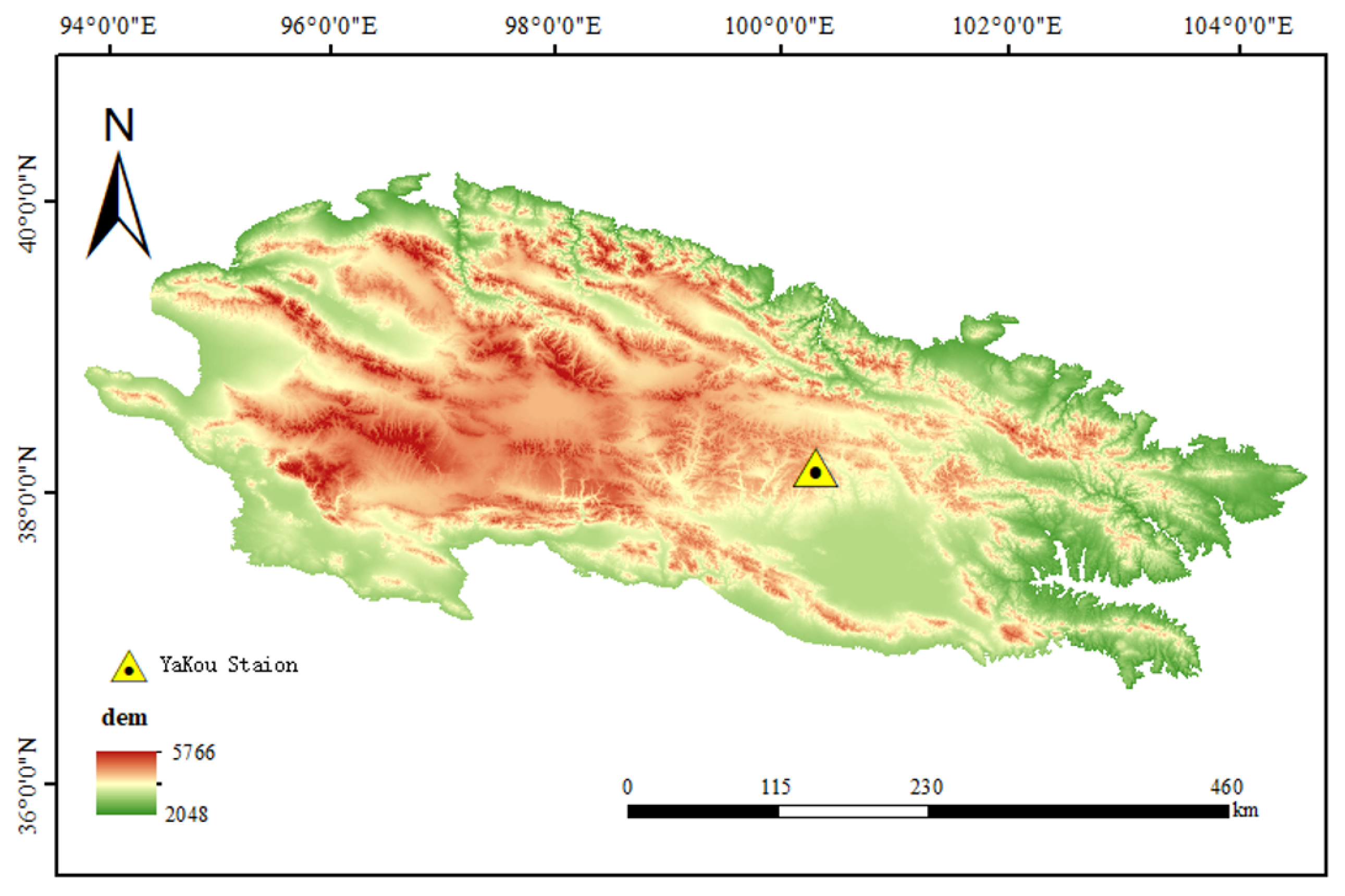
To address the above challenges, this study proposes an SWE reconstruction framework that integrates causal inference with machine learning. By incorporating causal relationships into feature selection, the proposed method aims to improve both reconstruction accuracy and physical interpretability [27]. Using the Dadongshu Yakou snow observation station in the Qilian Mountains as a representative case, this study investigates the response mechanisms between meteorological variables and SWE and evaluates the performance of multiple machine learning models, with LightGBM identified as the optimal approach. By applying the optimal model, we generated a high-precision and high-temporal-resolution Snow Water Equivalent (SWE) dataset spanning from 2018 to 2023. Furthermore, the Shapley Additive Explanations (SHAP) method was employed to quantify both the global and local contributions of each attribute. The main objectives of this study are as follows:

• To develop a high-precision, station-scale SWE reconstruction framework for alpine regions leveraging multi-source meteorological and snow observation data;
• To integrate causal inference (Granger causality) and correlation analysis for optimized feature selection, and to interpret model outputs via SHAP to enhance the understanding of underlying physical processes;
• To systematically evaluate the performance of various machine learning algorithms and identify the most suitable approach for SWE reconstruction in complex mountainous environments characterized by sparse observations.

2. Study Area and Data

2.1. Study Area

The study area is located in the Qilian Mountains, on the northeastern margin of the Qinghai–Tibet Plateau, spanning longitudes 93–105° E and latitudes 36–41° N, with elevations ranging from 2048 to 5766 m (see Figure 1). Characterized by a continental climate and typical plateau mountain climate features, the region experiences substantial snowfall during winter and spring, serving as a critical water source for the Heihe River Basin, Shule River Basin, and Shiyang River Basin. Snow cover is extensive, with frequent snowfall primarily occurring from October to May of the following year. The basins contain important snow observation stations, such as the Dadongshu Yakou Station, which facilitate detailed monitoring of snow conditions [28].

Temperature and precipitation are the primary drivers of snow cover changes, with spring variability sensitive to both, summer dominated by temperature, and winter influenced mainly by precipitation [29]. The Qilian Mountains feature cold, prolonged winters and short, cool summers with pronounced seasonal contrasts in temperature and precipitation (Figure 2a). From 2018 to 2023, monthly mean temperatures ranged from −15 °C (January) to 10 °C (July), with extremes from −25 °C to 30 °C. Precipitation is strongly seasonal, with more than 90% occurring between May and September (peaks: July 711.9 mm, August 786.7 mm), while the dry season (October–April) receives less than 5 mm per month. Snow cover exhibits marked seasonality and spatial heterogeneity (Figure 2b). Average snow depth peaks at 0.22–0.25 m in April–May, with extremes up to 0.55 m (May) and 0.45 m (November); summer values approach zero. SWE follows a similar pattern, peaking in April ( 60 mm) and November ( 65 mm), with negligible summer values. Higher SWE in November relative to snow depth indicates denser early-winter snow, whereas lower late-spring density causes a slight phase shift between snow depth and SWE maxima.

2.2. Data Sources

2.2.1. Ground-Based Observations

Ground-based station observations remain the most reliable benchmark for quantifying Snow Water Equivalent (SWE) [30]. In this study, in situ datasets were obtained from the Dadongshu Mountain YaKou station in the Qilian Mountains. The primary snow parameters, including snow depth (SD) and SWE, were monitored using a passive Gamma Monitoring (GMON/CS725) sensor. The measurement protocol leverages the principle of natural terrestrial gamma radiation attenuation. The sensor specifically monitors the energy photopeaks of ⁴⁰K (1.46 MeV) and ²⁰⁸Tl (2.61 MeV) emitted from the soil. By measuring the reduction in gamma-ray flux as it passes through the snowpack, the system provides a non-contact estimate of the total water mass.

The dataset utilized in this research spans six years (2018–2023). Snow depth was recorded at 30 min intervals, while SWE observations were integrated and recorded four times daily at six-hour intervals. To ensure data fidelity, the gamma counts were corrected for background soil moisture fluctuations using an integrated probe at a depth of 5 cm. These high-resolution recordings serve as a robust target for the machine learning reconstruction.

2.2.2. Reanalysis Data

ERA5 is the fifth-generation global atmospheric reanalysis dataset produced by the European Centre for Medium-Range Weather Forecasts (ECMWF). ERA5 provides a wide range of atmospheric, land, and oceanic climate variables at hourly intervals. Its spatial resolution is also high, with all atmospheric variables interpolated to a 0.25° × 0.25° grid. In this study, we used the daily SWE reanalysis dataset generated by ECMWF, which is available from 1981 to the present at a spatial resolution of 0.1° × 0.1°. The Global Land Data Assimilation System (GLDAS) dataset belongs to the category of land surface data assimilation products. It is generated by combining land surface models with multi-source observations, including satellite remote sensing and ground station data, rather than being a direct remote sensing observation. Its advantage lies in providing spatiotemporally continuous and physically consistent land surface hydrological and energy variables. The dataset has a spatial resolution of 0.25° × 0.25° and a temporal resolution of one day. In this study, we compared the daily SWE reanalysis dataset generated by ECMWF with the daily SWE dataset produced by GLDAS.

2.2.3. Meteorological Data

Meteorological data were obtained from the Dadongshu Yakou Station, operated by the Northwest Institute of Eco-Environment and Resources, Chinese Academy of Sciences. The dataset includes automatic weather station (AWS) and eddy covariance (EC) measurements from 2018 to 2023. The variables comprise air temperature and humidity, atmospheric pressure, precipitation, wind speed and direction, four-component radiation, surface radiative temperature, soil heat flux, soil temperature, and soil moisture. Preliminary preprocessing was conducted to remove duplicate records, eliminate values clearly beyond physical meaning or instrument ranges, and mark missing data with −6999. Both AWS and EC datasets provide 48 records per day, with measurements taken at 30 min intervals.

3. Methods

In recent years, machine learning models have been widely applied in fields such as snow remote sensing retrieval and numerical simulation of snowmelt runoff [31]. In this study, we developed a snow water equivalent (SWE) reconstruction method for alpine regions that integrates causal inference with machine learning (ML). The approach consists of three main stages. First, a hybrid feature selection strategy combining Granger causality inference and Pearson correlation analysis was employed to identify meteorological factors that exhibit both statistical correlations and causal relationships with SWE. These selected features were then used as inputs for the machine learning models. Second, eight commonly used machine learning algorithms—Support Vector Machine (SVM), ElasticNet, Bayesian Ridge Regression, Random Forest (RF), Extreme Gradient Boosting (XGBoost), Light Gradient Boosting Machine (LightGBM), CatBoost, and AdaBoost—were trained and systematically compared to construct the SWE reconstruction models, thereby enabling accurate estimation of SWE based on meteorological variables [32]. Finally, the optimally trained model was applied, together with meteorological factors, snow data, and other multi-source inputs, to reconstruct missing or anomalous SWE data.

The primary objective of this method is to achieve continuous, high-precision SWE reconstruction while elucidating the influential mechanisms between meteorological drivers and SWE variability.

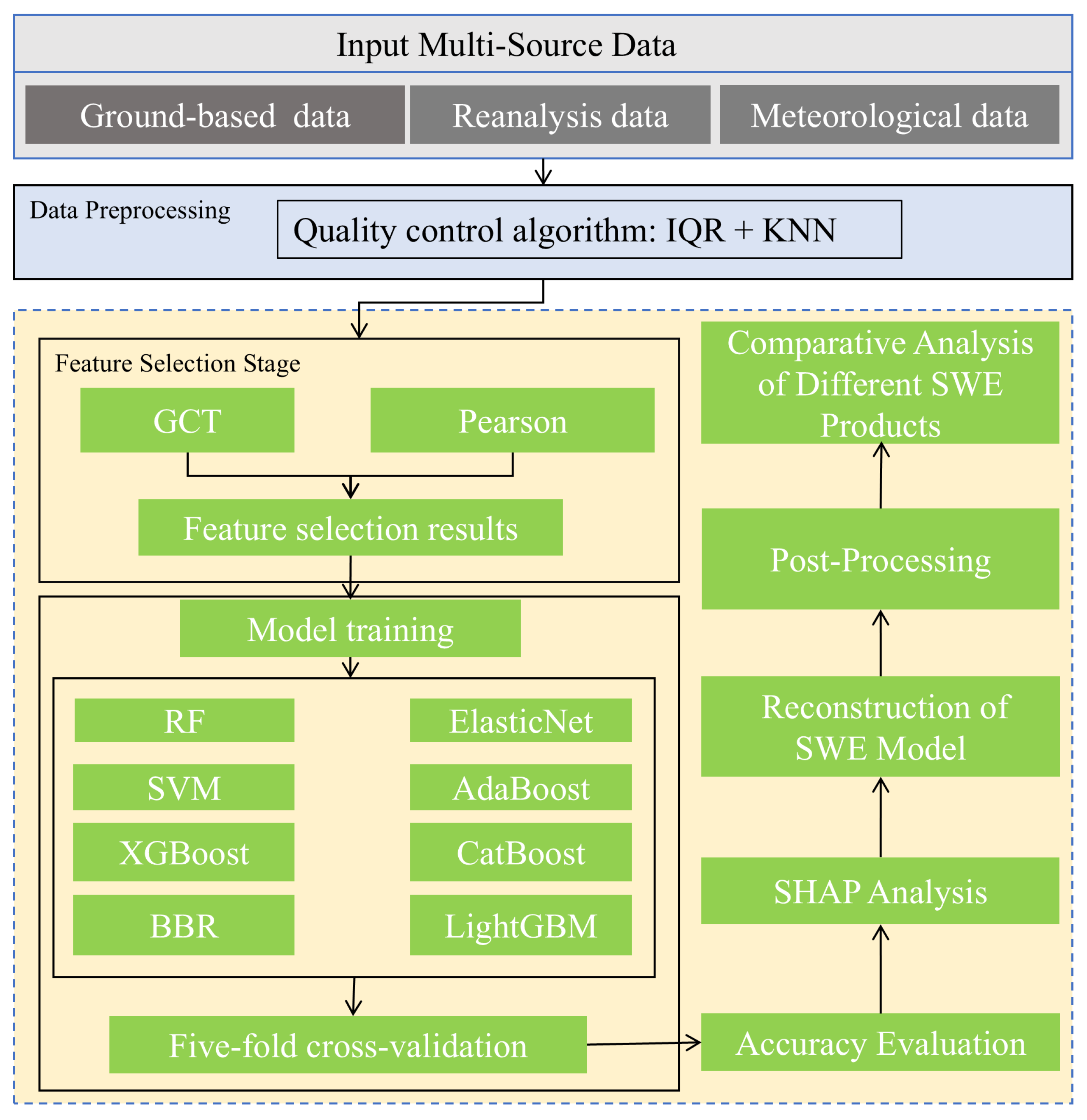
This study proposes a comprehensive SWE reconstruction framework based on multi-source data fusion and machine learning (ML) modeling in complex terrain(see Figure 3). The framework comprises the following stages: (1) Data preparation—integration of multi-source inputs, including in situ snow observations, reanalysis datasets, and meteorological variables. Preprocessing includes quality control using IQR and KNN algorithms to remove outliers and handle missing values. (2) Feature selection—application of Granger causality tests (GCT) combined with Pearson correlation analysis to identify meteorological factors that exhibit both causal relationships and statistical correlations with SWE. (3) Model development and training—systematic training and evaluation of eight ML algorithms (SVM, ElasticNet, Bayesian Ridge Regression, Random Forest, XGBoost, LightGBM, CatBoost, and AdaBoost) using five-fold cross-validation to construct SWE reconstruction models. (4) Model validation and interpretability—accuracy assessment of the models through five-fold cross-validation, followed by SHAP analysis to interpret the contribution of individual features. (5) Reconstruction and post-processing—application of the optimal model to downscale and reconstruct SWE time series, correction of anomalies, and comparative analysis with existing SWE products.

This integrated framework provides an effective and interpretable approach for SWE estimation in complex mountainous environments, with potential applications in water resource management and hydrological forecasting.

3.1. Feature Selection Method

3.1.1. Pearson

The Pearson Correlation Coefficient (PCC) is a widely used statistical measure that quantifies the strength and direction of the linear relationship between two variables, with values ranging from −1 to +1. A coefficient close to +1 indicates a strong positive linear correlation (both variables increase together), whereas a value near −1 signifies a strong negative linear correlation (one variable increases as the other decreases). Values around 0 imply little to no linear association.

Mathematically, the PCC is derived by normalizing the covariance of the two variables by the product of their standard deviations, thereby providing a scale-independent measure of linear dependence. Due to its computational simplicity and interpretability, the PCC is commonly employed in exploratory data analysis and feature selection tasks.

However, it is limited to detecting linear relationships only and can be sensitive to outliers and non-linear associations.

The Pearson Correlation Coefficient (PCC), denoted as ${\rho }_{X,Y}$ (population) or $r_{X,Y}$ (sample), measures the strength and direction of the linear relationship between two variables X and Y. It is defined as the covariance of the variables divided by the product of their standard deviations:

$${\rho }_{X,Y}={\displaystyle \frac{Cov(X,Y)}{{\sigma }_X{\sigma }_Y}},$$

(1)

where $Cov(X,Y)$ is the covariance, and ${\sigma }_X$ and ${\sigma }_Y$ are the standard deviations of X and Y, respectively.

For a sample of size n, the sample Pearson correlation coefficient r is computed as:

$$r={\displaystyle \frac{{\sum }_{i=1}^n(x_i-\overline{x})(y_i-\overline{y})}{\sqrt{{\sum }_{i=1}^n{(x_i-\overline{x})}^2}\sqrt{{\sum }_{i=1}^n{(y_i-\overline{y})}^2}}},$$

(2)

where $\overline{x}$ and $\overline{y}$ are the sample means of X and Y.

This formulation ensures that r ranges from −1 to +1, with the same interpretive properties described earlier. In this study, the sample Pearson correlation coefficient was calculated for each meteorological variable against SWE to identify linearly associated features prior to causal inference.

3.1.2. Granger Causality Test (GCT)

The Granger Causality Test (GCT) was employed to identify causal relationships between meteorological variables and Snow Water Equivalent (SWE). GCT is a statistical approach for causal inference in time series data, based on predictive improvement. Specifically, a variable X is said to Granger-cause Y if past values of X provide statistically significant information about future values of Y, beyond that provided by the past values of Y alone [33].

A key prerequisite for a valid GCT application is stationarity of the time series, as non-stationary data can lead to spurious regression results. Therefore, the Augmented Dickey–Fuller (ADF) test was first applied to verify the stationarity of each variable. Non-stationary series were differenced until stationarity was achieved.

The hypothesis testing framework is as follows:

Null hypothesis ($H_0$): X does not Granger-cause Y (i.e., lagged values of X contribute no additional explanatory power to the prediction of Y). Alternative hypothesis ($H_1$): X Granger-causes Y.

The test is typically performed using an autoregressive model that includes lagged terms of both Y and X, with statistical significance assessed via an F-test on the coefficients of the lagged X terms. In this study, GCT was combined with Pearson correlation analysis to select features exhibiting both strong linear association and causal influence on SWE.

3.2. Machine Learning Models for Snow Water Equivalent (SWE) Reconstruction

Machine learning (ML) methods have shown superior performance in snow cover remote sensing and SWE reconstruction due to their ability to capture complex nonlinear relationships among meteorological variables, topographic features, and microwave signals [34]. To identify the most suitable approach for alpine regions with high spatiotemporal heterogeneity, eight state-of-the-art ML regression algorithms were selected and compared in this study: ElasticNet, Bayesian Ridge Regression (BRR), Random Forest (RF), AdaBoost, XGBoost, LightGBM, CatBoost, and Support Vector Regression (SVM). These models represent diverse methodological paradigms—regularization-based linear models (ElasticNet, BRR), kernel-based methods (SVM), bagging ensembles (RF), and boosting ensembles (AdaBoost, XGBoost, LightGBM, CatBoost)—and have demonstrated strong performance in high-dimensional hydrological prediction tasks [35]. Comprehensive comparison enables robust identification of the optimal model for SWE reconstruction.

The dataset adopted in this study covers a six-year time span from 2018 to 2023, consisting of daily observations obtained from a single observation station. Specifically, the dataset contains 4 daily SWE records and 48 daily observations of different meteorological variables. Unlike traditional time-series prediction tasks that highly rely on temporal continuity, the core of the SWE reconstruction task in this study is to capture the nonlinear relationship between snow dynamics and meteorological driving factors [36]. The data division strategy in this study is as follows: 80% of the data is used for training, and the remaining 20% is used for testing. Based on the principle of five-fold cross-validation, the samples are randomly divided into five subsets and repeated five times. Each round involves training the model on four subsets and using the last subset to verify the model’s effectiveness. All results are aggregated to evaluate model performance and reduce the bias caused by a specific validation set. This method is suitable for small sample scenarios because it allows the repeated use of randomly generated subsamples for training and validation.

Brief descriptions of the eight models are provided below to highlight their methodological diversity and suitability for SWE reconstruction.

• Support Vector Regression (SVR) [37]: A kernel-based nonlinear regression method that maps input variables into a high-dimensional feature space using kernel functions, enabling the modeling of complex nonlinear relationships between meteorological variables and SWE.
• Bayesian Ridge Regression (BRR): A probabilistic linear regression model that introduces prior distributions over regression coefficients and updates them using Bayes’ theorem, providing stable parameter estimation for baseline SWE modeling.
• ElasticNet [38]: A linear regression model with combined $L_1$ and $L_2$ regularization, where feature coefficients are jointly optimized to improve generalization and handle multicollinearity among meteorological predictors.
• Random Forest (RF) [39]: An ensemble learning method that constructs multiple decision trees using bootstrap sampling and averages their outputs, reducing variance and improving robustness in nonlinear SWE estimation.
• AdaBoost [40]: A boosting algorithm that sequentially trains weak learners while increasing the weight of poorly predicted samples, thereby improving model focus on difficult SWE patterns.
• XGBoost [40]: A gradient boosting framework that optimizes a regularized objective function using first- and second-order gradients, enabling accurate modeling of nonlinear interactions in SWE drivers.
• CatBoost [41]: A gradient boosting method that reduces prediction bias through ordered boosting, improving generalization performance on heterogeneous meteorological datasets.
• LightGBM [42]: A gradient boosting model that grows trees in a leaf-wise manner and uses histogram-based splitting, improving computational efficiency and capturing complex nonlinear relationships in SWE reconstruction.

Through systematic comparison, the optimal model was identified and further interpreted using Shapley Additive Explanations (SHAP) to quantify feature contributions to SWE reconstruction.

3.3. Model Evaluation

To ensure robust and reliable performance assessment, this study employed 5-fold cross-validation. The dataset was randomly partitioned into five equally sized subsets. In each fold, four subsets were used for training and the remaining one for validation, with the process repeated five times such that each subset served as the validation set exactly once. The final performance metrics were computed as the average across all five folds. This approach maximizes data utilization, mitigates overfitting risks by exposing the model to different training–validation splits, and yields more stable and generalizable estimates of model performance compared to a single train–test split.

Model performance was quantified using three widely accepted statistical metrics: the coefficient of determination ($R^2$), root mean squared error (RMSE), and mean absolute error (MAE). $R^2$ represents the proportion of variance in the observed SWE explained by the model, with values closer to 1 indicating superior fit and values near or below 0 suggesting poor predictive capability. RMSE provides a measure of the average magnitude of prediction errors in the original units, with greater sensitivity to larger errors due to squaring. MAE quantifies the average absolute deviation between predicted and observed values, offering a more intuitive interpretation of typical error magnitude. Lower values of RMSE and MAE indicate higher predictive accuracy.

The mathematical formulations are as follows:

$$\mathrm{MAE}={\displaystyle \frac{1}{n}}{\displaystyle \sum _{i=1}^n}\left|y_i-{\widehat{y}}_i\right|,$$

(3)

$$\mathrm{RMSE}=\sqrt{{\displaystyle \frac{1}{n}}\sum _{i=1}^n{(y_i-{\widehat{y}}_i)}^2},$$

(4)

$$R^2=1-{\displaystyle \frac{{\sum }_{i=1}^n{(y_i-{\widehat{y}}_i)}^2}{{\sum }_{i=1}^n{(y_i-\overline{y})}^2}},$$

(5)

where $y_i$ is the observed SWE value, ${\widehat{y}}_i$ is the predicted value, $\overline{y}$ is the mean of the observed values, and n is the number of samples.

These metrics collectively provide a comprehensive evaluation of both accuracy and explanatory power, enabling fair comparison across the six machine learning models.

4. Result

4.1. Analysis of Feature Selection Results

The Granger Causality Test (GCT) was applied to identify meteorological variables that causally influence Snow Water Equivalent (SWE). GCT evaluates whether lagged values of a predictor variable X provide statistically significant information for forecasting Y (here, SWE) beyond that contained in the lagged values of Y alone. To account for potential delayed responses in snow accumulation and ablation processes, five lag periods (1 to 5 days) were tested. For each meteorological variable, GCT was performed with SWE as the target (effect) variable. The null hypothesis ($H_0$) states that the predictor does not Granger-cause SWE (i.e., its lagged values have no predictive power). Rejection of $H_0$ is indicated by low p-values, signifying stronger evidence of a causal relationship.

Results from the Granger Causality Test (GCT), as shown in Figure S1 (Supplementary Materials), indicate that several variables—including deep soil temperature, soil moisture, instrument voltage, and wind speed—yielded high p-values. This suggests their causal influence on SWE is statistically insignificant, justifying their exclusion from the final model input. In contrast, precipitation, surface soil temperature and moisture, and snow depth yield extremely low p-values across multiple lags, demonstrating strong causal relationships with SWE variations. These variables primarily drive SWE variations through water input, energy balance, and snowpack retention processes, consistent with established snow hydrological mechanisms. For clarity and readability, detailed Granger causality test results (including lag-specific p-value distributions) are provided in the Supplementary Material, rather than the main text.

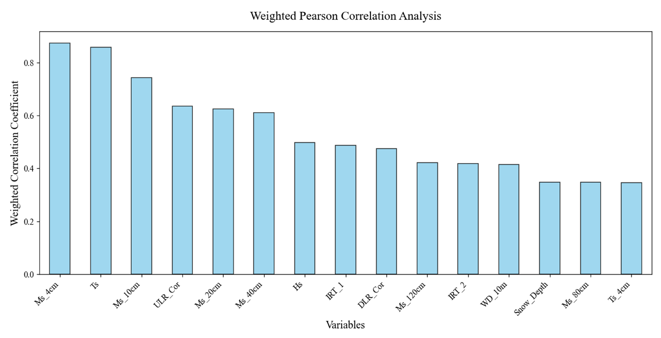
Since GCT primarily captures causality but does not quantify the strength of linear association, Pearson correlation analysis was conducted as a complementary step to assess linear relationships between predictors and SWE. Through the Pearson feature importance analysis illustrated in Figure 4, it can be observed that shallow soil temperature and moisture exhibit strong correlations with SWE. Radiation-related variables show moderate correlations, while deep soil temperature and moisture, together with snow depth, also demonstrate certain degrees of association.

The combined results show that snow depth, precipitation, and surface soil temperature and moisture not only exhibit strong linear correlations but also clear causal linkages with SWE. These variables were therefore prioritized as key features for the subsequent machine learning models. Conversely, variables with weak causality and low correlation (e.g., wind direction and deep soil parameters) were excluded, thereby reducing model complexity and mitigating overfitting risks while preserving predictive performance.

4.2. Machine Learning Model Performance

To evaluate the applicability and predictive accuracy of different machine learning (ML) methods for snow water equivalent (SWE) reconstruction in the Qilian Mountains, a comprehensive comparative assessment was conducted across eight ML models: ElasticNet, Bayesian Ridge Regression (BRR), Random Forest (RF), AdaBoost, XGBoost, LightGBM, CatBoost, and Support Vector Regression (SVR).

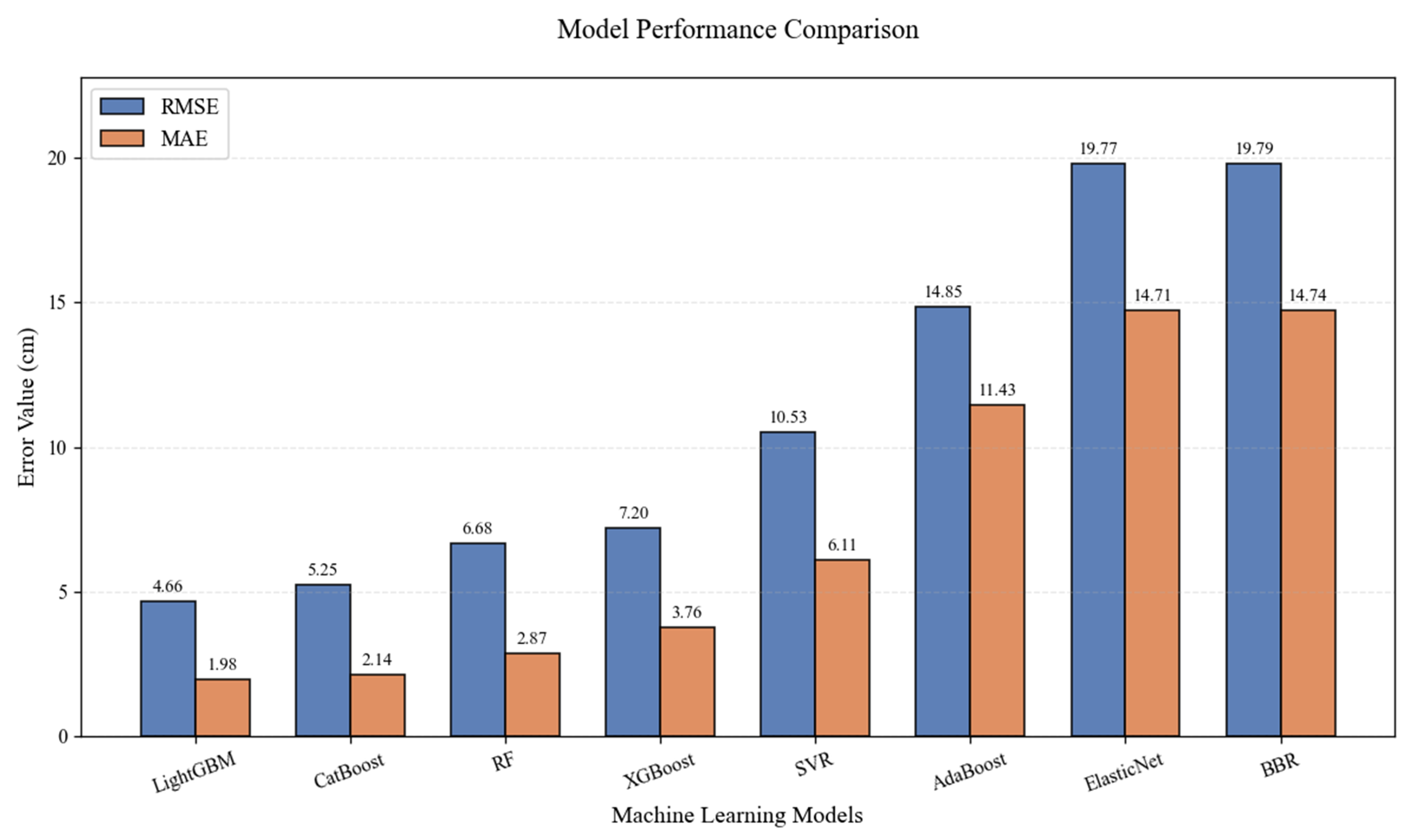
Model performance was quantitatively evaluated using three standard metrics: mean absolute error (MAE), root mean squared error (RMSE), and coefficient of determination ($R^2$). As shown in Figure 5, LightGBM achieved the best overall performance, with the lowest RMSE and MAE values and the highest $R^2$, indicating its superior ability to capture the complex nonlinear dynamics that govern SWE variability in alpine environments. Gradient boosting-based models (LightGBM, CatBoost, XGBoost) consistently outperformed traditional methods such as Random Forest (RF), Support Vector Regression (SVR), ElasticNet, and Bayesian Ridge Regression (BRR) in SWE reconstruction.

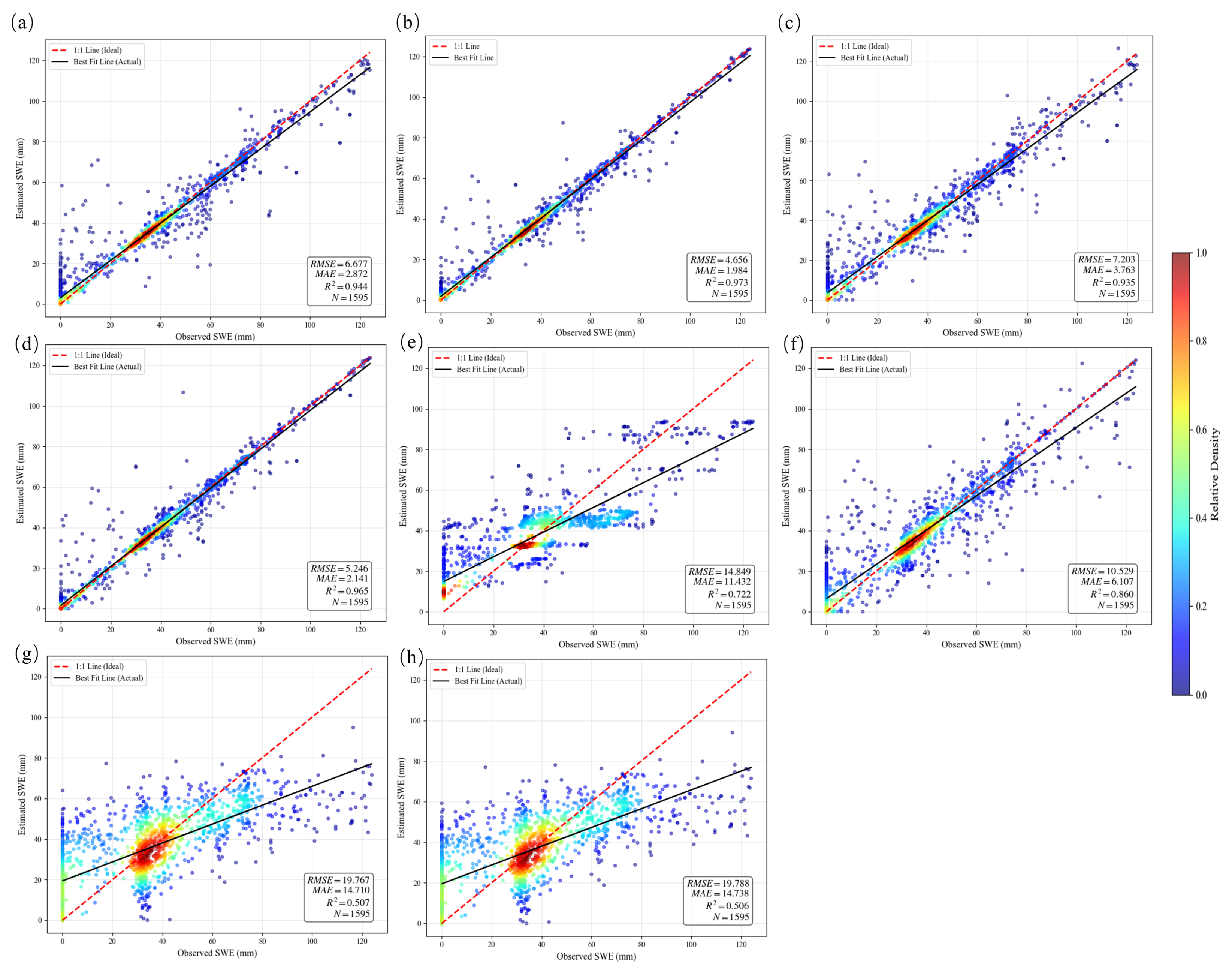
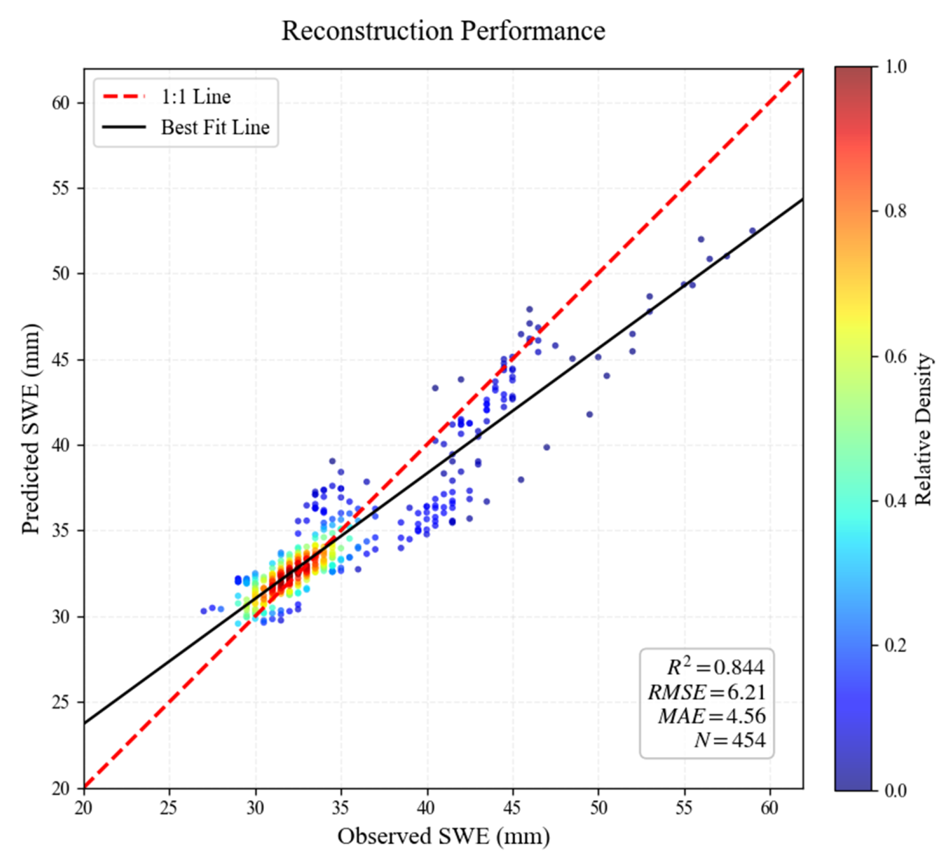
To evaluate the fitting performance of the eight machine learning models on the test dataset, scatter plots were generated based on the predicted values and corresponding ground truth observations (see Figure 6). These plots clearly illustrate the degree of agreement between model predictions and actual SWE measurements.

CatBoost’s advantage lies in its ordered boosting mechanism, which reduces prediction bias and target leakage, thereby improving bias control and robustness. However, its sensitivity to hyperparameter settings makes it slightly less stable than LightGBM. Random Forest, while exhibiting somewhat larger fluctuations, produced relatively uniform error distributions and maintained high overall accuracy. As a bagging-based ensemble method, it mitigates overfitting through the voting mechanism of multiple decision trees, though it is less effective than gradient boosting models in capturing high-dimensional feature interactions. The relatively larger errors of XGBoost can be attributed to its lower efficiency in modeling SWE heterogeneity under complex terrain compared to LightGBM. AdaBoost, being highly sensitive to outliers, struggled with the complex coupling among meteorological variables, resulting in larger prediction fluctuations and errors.

Methods such as SVR, Bayesian Ridge Regression (BRR), and ElasticNet are inherently limited in their ability to capture the nonlinear dynamics of SWE in mountainous regions. Consequently, their predictions showed substantial deviations, unstable trends, and pronounced errors, making them unsuitable for SWE reconstruction in complex alpine environments.

Based on the accuracy metrics presented in

Table 1. Performance comparison of the eight machine learning models for SWE reconstruction on the test dataset.

Model	RMSE (mm)	MAE (mm)	${\mathit{R}}^2$
LightGBM	4.656	1.984	0.973
CatBoost	5.246	2.141	0.965
Random Forest (RF)	6.677	2.872	0.944
XGBoost	7.203	3.763	0.935
Support Vector Regression (SVR)	10.529	6.107	0.860
AdaBoost	14.849	11.432	0.722
ElasticNet	19.767	14.710	0.507
Bayesian Ridge Regression (BBR)	19.788	14.738	0.506

and the distribution characteristics of prediction errors, a comprehensive analysis was conducted across the eight machine learning models. Regarding error magnitude, gradient boosting decision tree (GBDT) architectures exhibited significantly lower errors compared to other approaches. LightGBM achieved the highest predictive precision, with an RMSE of 4.656 mm, MAE of 1.984 mm, and $R^2=0.973$, indicating minimal deviation between predicted and observed values. CatBoost yielded performance comparable to LightGBM, with an RMSE of 5.246 mm, MAE of 2.141 mm, and $R^2=0.965$, although its error margin slightly increased in certain high-value prediction intervals.

In contrast, other boosting-based and ensemble methods showed noticeably higher errors. Specifically, XGBoost and RF yielded RMSE values of 7.203 mm and 6.677 mm, respectively, while AdaBoost and SVR demonstrated even greater deviations, with RMSE values exceeding 10 mm and significantly reduced $R^2$ values ($R^2=0.722$ and $0.860$, respectively). These results underscore that while all GBDT models generally perform well, LightGBM and CatBoost are superior in capturing the complex nonlinear dynamics governing SWE variability in the Qilian Mountains.

From the analysis of error distributions and $R^2$ values, it can be concluded that LightGBM and CatBoost hold distinct advantages in reproducing the spatiotemporal variability of SWE. The gradient boosting framework excels at learning multidimensional interactions, making it particularly effective in capturing the nonlinear coupling among snow depth, precipitation, temperature, and soil conditions in typical mountainous environments. Furthermore, LightGBM combines high predictive accuracy with computational efficiency, rendering it highly suitable for SWE reconstruction and regional-scale monitoring in alpine regions.

4.3. Machine Learning Model Reconstruction Results

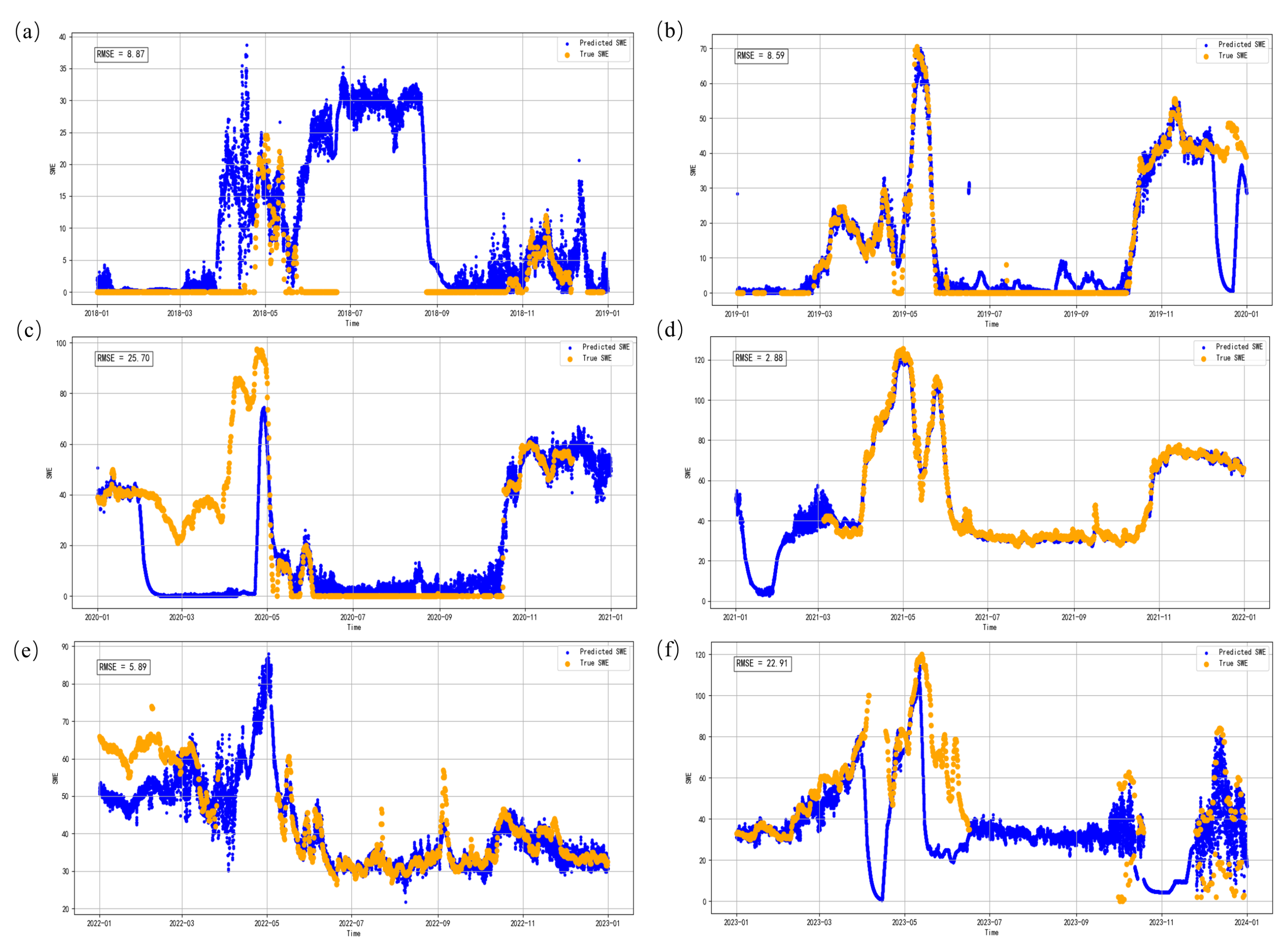
The differences in RMSE across years are pronounced, indicating that the predictive capability of the models is not stable over time. In

Table 2. Yearly RMSE comparison before and after outlier removal.

Year	RMSE	RMSE After Outlier Removal
2018	9.40	8.87
2019	10.10	8.59
2020	26.77	25.70
2021	3.13	2.88
2022	6.14	5.89
2023	24.83	22.91

, the overall RMSE ranges from approximately 2.88 to 26.77, with the minimum value observed in 2021 and the maximum in 2020. This suggests that model performance varies considerably under different climatic conditions and data contexts.

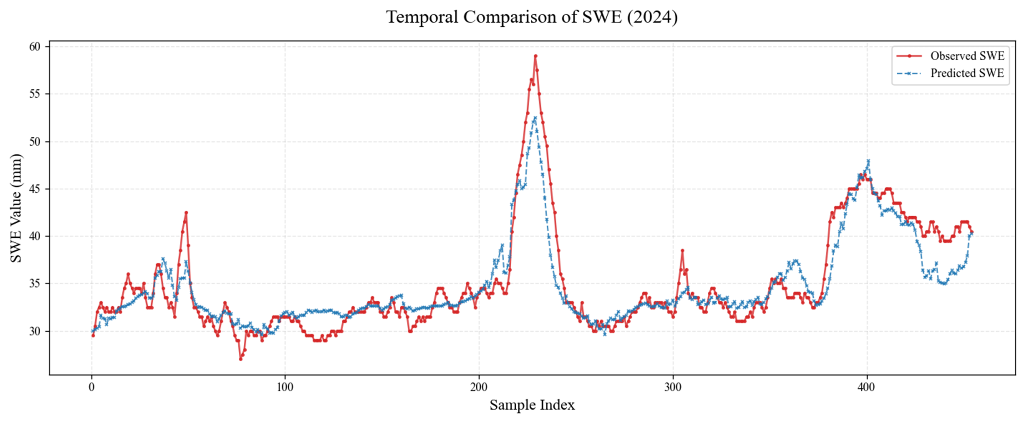
From the interannual variation shown in Figure 7, the errors exhibit a strong correspondence with the SWE dynamics. In 2018, the RMSE was 9.40, representing a moderate level. SWE fluctuations were relatively frequent but with low peak values, and the models were able to generally follow the trend, though local variations were not well captured. In 2019, the RMSE increased slightly to 10.10, close to 2018, but with more pronounced SWE rises and abrupt changes, leading to deviations during rapid transitions. In 2020, the RMSE reached the highest value of 26.77, reflecting large SWE variations with steep increases and sudden drops, which the models struggled to capture, resulting in significantly higher errors.

In 2021, the RMSE dropped to the lowest value of 3.13, indicating the best model performance. SWE changes were relatively smooth, with moderate peaks and continuous rising and falling processes, allowing the models to learn the dynamics more accurately. In 2022, the RMSE increased to 6.14, higher than in 2021 but still at a relatively good level. SWE showed some fluctuations but fewer extreme changes. In 2023, the RMSE rose again to 24.83, suggesting a clear decline in model performance. That year, SWE exhibited high peaks and frequent fluctuations in the later period, with localized sharp oscillations, which increased prediction difficulty.

From the existing analysis, it can be summarized that model performance is mainly influenced by three factors: first, the intensity of interannual variability, with larger fluctuations leading to greater errors; second, the distribution of extreme values, where the presence of more extremes has a pronounced impact on RMSE; and third, data integrity, as missing or anomalous data weaken the model’s learning capability. Therefore, it can be concluded that the models achieve the highest accuracy in stable years, while years characterized by high volatility and poor data quality still exhibit significant limitations. Strengthening outlier handling, missing data imputation, and the ability to model extreme variations is essential to improving the generalization performance and stability of the models under complex conditions.

4.4. Validation Using Simulated Missing Data

Data from mountain ground stations are often subject to missing values due to equipment failures or severe weather conditions. To evaluate the reconstruction capability of the model under scenarios of data loss, we artificially masked different proportions of the observations (simulating missing data) and used the LightGBM model to predict the missing values. The predicted values were then compared with the actual observations to assess the reconstruction accuracy. Two types of missing data were considered: random missing data at rates of 5%, 10%, 15%, and 30%, and continuous missing segments (six consecutive periods) at rates of 5%, 10%, and 15%.

According to

Table 3. Reconstruction accuracy of LightGBM under different missing data scenarios.

Missing Pattern	Missing Rate	MAE (mm)	RMSE (mm)
Random Missing	5%	0.58	1.17
Random Missing	10%	0.63	1.30
Random Missing	15%	0.65	1.33
Random Missing	30%	0.72	1.57
Continuous Missing	5%	0.61	1.22
Continuous Missing	10%	0.67	1.38
Continuous Missing	20%	0.75	1.62

, under the random missing pattern with a missing rate of 5%, the model achieved a mean absolute error (MAE) of 0.58 mm and a root mean square error (RMSE) of 1.17 mm. Under the continuous missing pattern with the same missing rate, the MAE was 0.61 mm and the RMSE was 1.22 mm. As the missing rate increased, the model errors showed a gradual upward trend, though the overall increase remained relatively small. This verifies the reliability of the model in scenarios with missing data and demonstrates its suitability for data reconstruction tasks at mountain stations.

4.5. Validation Against Multi-Source Satellite and Reanalysis Products

To evaluate the effectiveness and reliability of the proposed SWE reconstruction model, its performance was compared with three benchmark products, including ERA5-Land, GLDAS, and SWE derived from the snow density product. For the latter, SWE was calculated based on ground station snow depth observations and a fixed snow density of 0.3 g/cm³. All comparisons were conducted for the 2019–2020 snow season, using in situ measurements from the Dadongshu Yakou station as ground truth.

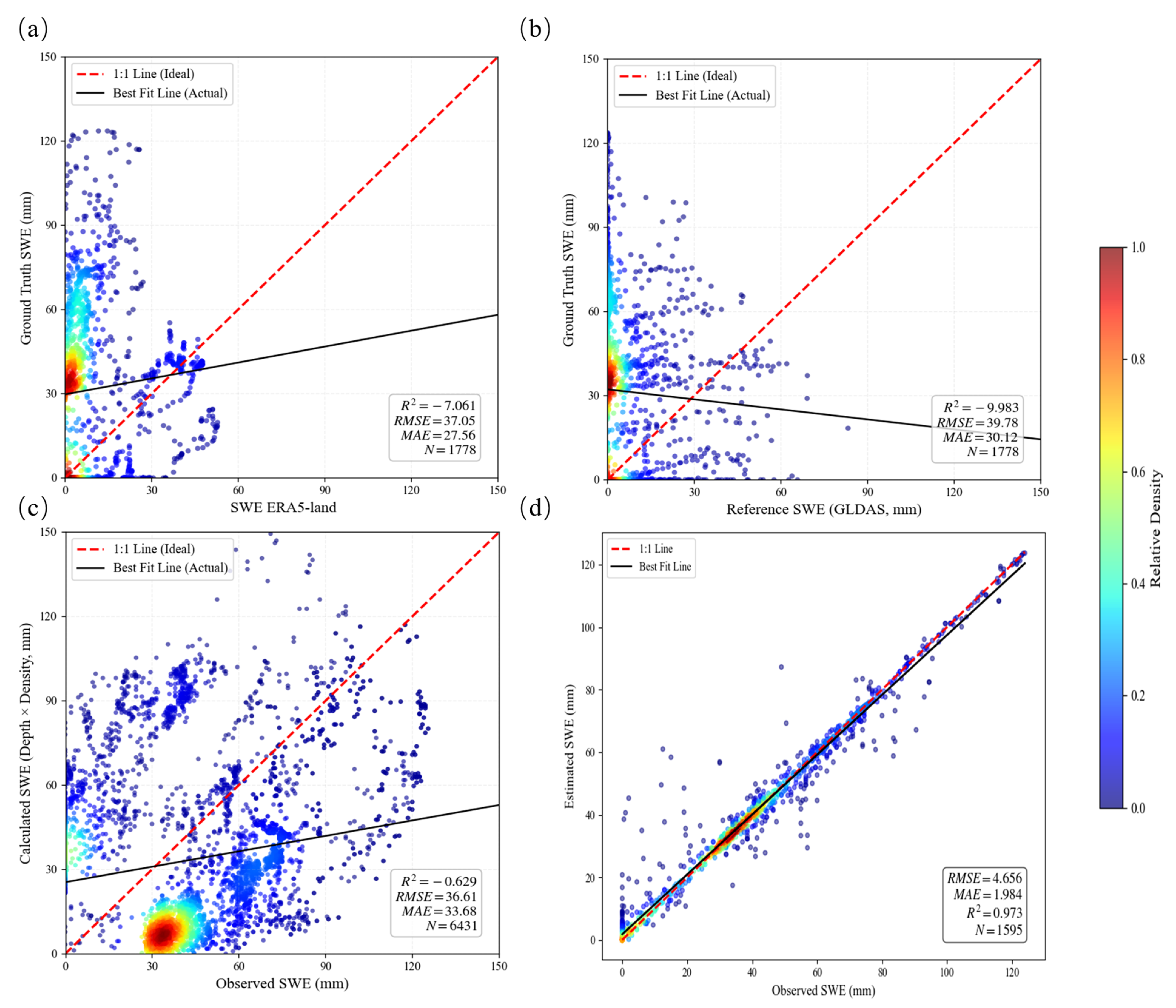
As shown in

Table 4. Accuracy comparison between multi-source SWE products and the reconstructed data in this study.

Product	MAE	RMSE	Correlation Coefficient (${\mathit{R}}^2$)
LightGBM	1.98	4.66	0.97
ERA5-Land	27.55	37.05	0.49
GLDAS	29.32	39.17	0.45
Snow density product	8.67	12.34	0.83

, the LightGBM-based SWE reconstruction proposed in this study achieves a higher level of accuracy compared to existing reanalysis products and empirical methods. On the test dataset, the model yields a correlation coefficient of 0.97, with an MAE of 1.98 mm and an RMSE of 4.66 mm, indicating a high degree of consistency between the predicted values and in situ observations.

In contrast, the SWE data derived from the conventional snow depth–density product (Figure 8c) exhibits larger errors, with an RMSE of 12.34 mm. Although this approach captures the general accumulation trends, its reliance on a fixed density assumption (0.3 g/cm³) fails to account for the dynamic densification processes influenced by temperature and snowpack metamorphism.

Furthermore, the ERA5-Land and GLDAS products (Figure 8a,b) show even more pronounced discrepancies, with MAE values exceeding 27 mm and $R^2$ values falling below 0.5. These errors primarily stem from their coarse spatial resolutions (0.1–0.25°), which struggle to resolve the complex spatial heterogeneity and steep topographic gradients of the Qilian Mountains. Additionally, systematic biases in the underlying snow physics schemes of these products lead to underestimations of peak SWE values.

Overall, by integrating high-resolution station data with causality-driven feature selection, the proposed model effectively captures the nonlinear dynamics of SWE. Its RMSE of 4.656 mm is significantly lower than those of mainstream reanalysis products and simplified empirical methods, verifying its reliability for high-precision SWE reconstruction in complex mountainous regions.

Figure 8 provides a clear visualization of the consistency among different data sources at the regional scale, highlighting the pronounced differences in SWE reconstruction performance. GLDAS shows poor consistency with observations and fails to reflect the actual variations. ERA5-Land is able to capture the overall trend, but its RMSE remains large, with evident deviations in periods of fluctuations or extreme values. The snow depth–density product, constrained by the assumption of a fixed density, demonstrates limited fitting performance and exhibits substantial deviations from the observations in certain intervals. In contrast, the LightGBM model achieves the best performance, effectively capturing the nonlinear dynamics of SWE. Overall, the machine learning approach based on causality-driven feature selection proposed in this study demonstrates superior accuracy and stability compared with traditional reanalysis products and simplified calculation methods, thereby verifying its reliability and application potential for SWE reconstruction in complex regions.

4.6. Model Interpretability Using SHAP Analysis

Machine learning models generally possess strong nonlinear representation capabilities, yet their inherent “black-box” nature often limits the transparency of their internal decision-making mechanisms. To clarify the decision logic of the LightGBM model for SWE reconstruction and to analyze the specific influence of various meteorological factors, this study employs the SHAP (Shapley Additive Explanations) method for attribution analysis.

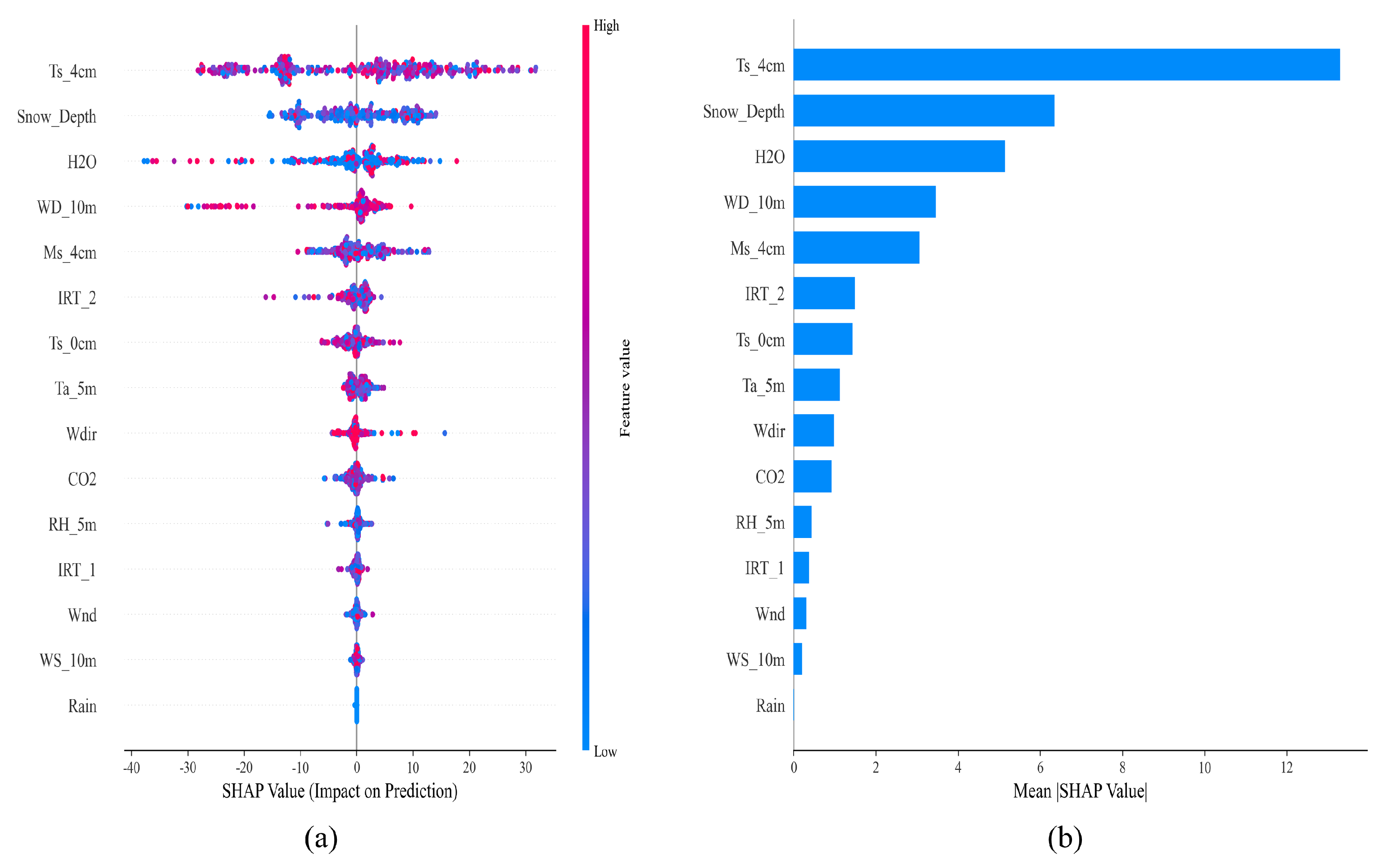
Figure 9 provides a comprehensive interpretability analysis of the LightGBM model. Specifically, Figure 9b ranks the input features based on their mean absolute SHAP values, offering a quantitative measure of each predictor’s global contribution to the SWE reconstruction. The results identify shallow soil temperature (Ts_4cm) as the most critical predictor, followed by snow depth (Snow_Depth) and soil moisture (H₂O), emphasizing the dominant role of the underlying surface’s thermal and hydrological states in governing snowpack dynamics.

Furthermore, the SHAP summary plot in Figure 9a illustrates the distribution of the impact of each feature on the model output, revealing the underlying physical mechanisms. Snow depth and soil moisture exhibit a significant positive gain effect on SWE, reflecting how material availability and ground-level humidity support snowpack maintenance. In contrast, the impact of soil temperature reflects a clear thermodynamic response: lower soil temperatures correspond to positive SHAP values, which favor stable snow accumulation, while higher temperatures significantly accelerate snow ablation. These findings are highly consistent with the physical processes of snow dynamics in high-altitude mountainous regions, indicating that the proposed model not only achieves high predictive accuracy but also maintains robust physical interpretability by prioritizing meaningful environmental precursors over secondary meteorological noise.

Figure 9b illustrates the global importance ranking of the input features based on their mean absolute SHAP values, providing a quantitative measure of each predictor’s overall contribution to the SWE reconstruction. The results identify shallow soil temperature (Ts_4cm) as the most critical predictor, followed by snow depth (Snow_Depth) and soil moisture (H₂O). Specifically, the high mean absolute SHAP value for Ts_4cm highlights that the energy exchange at the soil–snow interface is the primary driver of snow phase changes and persistence. By aggregating the global impact of each variable, Figure 9b confirms that the model prioritizes physically meaningful precursors over secondary meteorological noise, ensuring the reliability of the reconstructed SWE time series.

4.7. Hyperparameter Sensitivity Analysis for the LightGBM Model

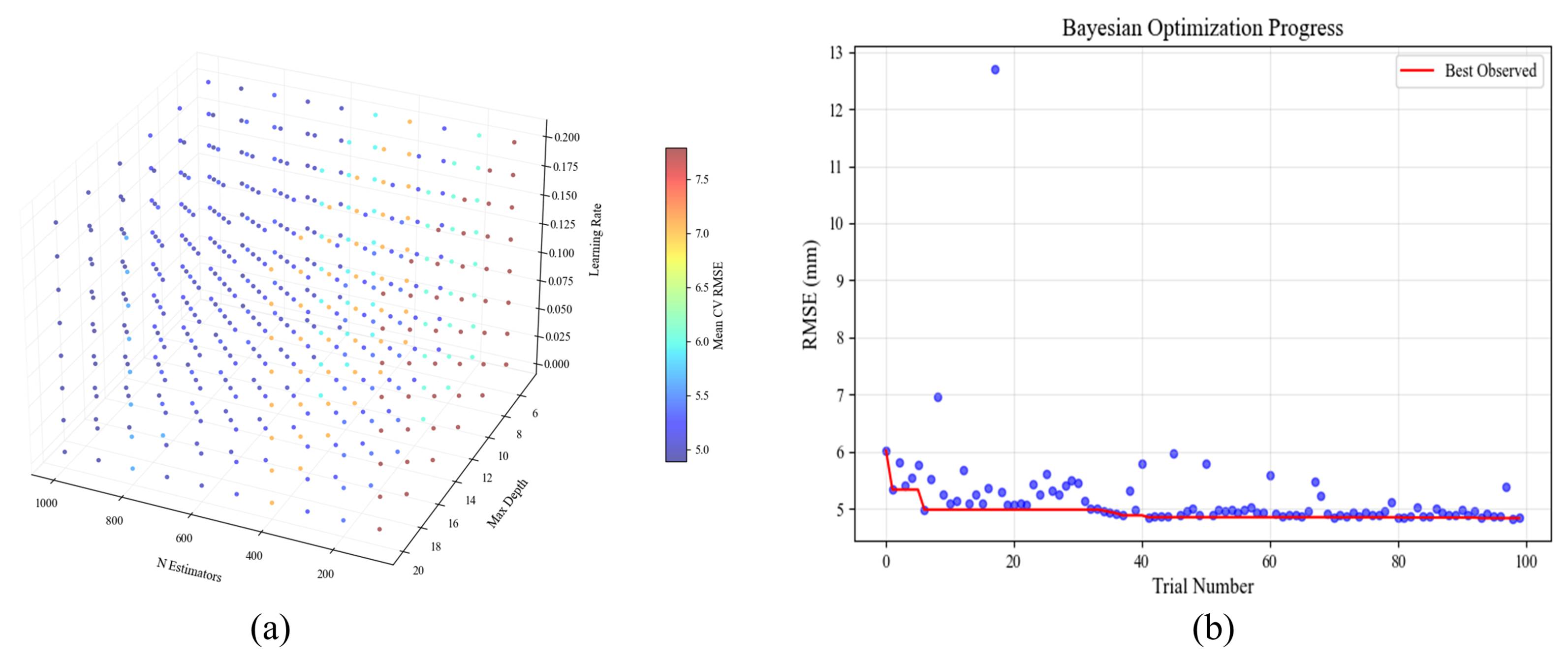
The hyperparameters of the LightGBM model were optimized using a Bayesian optimization strategy implemented through the Optuna framework, combined with five-fold cross-validation to ensure robust parameter selection. Several key hyperparameters were considered, including learning_rate, max_depth, and n_estimators, alongside regularization parameters such as num_leaves and min_child_samples.

As illustrated in Figure 10a, the three-dimensional visualization of the hyperparameter space reveals the sensitivity of the model performance (Mean CV RMSE) to the interaction between n_estimators, max_depth, and learning_rate. The color gradient indicates a clear convergence towards a low-RMSE region (blue clusters), predominantly located at moderate to high n_estimators and relatively lower learning_rate. Specifically, the model exhibits higher stability when learning_rate is maintained between 0.01 and 0.05, while performance degrades (red regions) as the learning rate increases beyond 0.15, regardless of tree depth.

The convergence behavior of the Bayesian optimization is depicted in Figure 10b. The optimization process shows rapid initial convergence, with the objective function (RMSE) stabilizing significantly after approximately 40 trials. The gap between the individual trial results (blue dots) and the best observed objective value (red line) progressively narrows, indicating an efficient exploration–exploitation balance within the Optuna framework.

Based on the optimization results, the optimal hyperparameter configuration was identified as: learning_rate = 0.017, max_depth = 18, and n_estimators = 723. This combination achieved a minimum cross-validation RMSE of approximately 4.85 mm (0.485 cm), demonstrating that the LightGBM model is capable of reaching a stable and globally optimal solution within the defined search space.

5. Discussion

5.1. Independent Validation and Model Robustness Analysis

To further assess the generalization ability of the proposed model, an independent validation was conducted using an unseen dataset from March to May 2024, corresponding to the critical snowmelt period. Due to sensor maintenance, observations from early winter were not available. As shown in Figure 11, the model maintains stable predictive performance under pronounced seasonal variability, indicating strong robustness in capturing rapid snowmelt dynamics. The model achieves an $R^2$ of 0.844, with an $RMSE$ of $6.21\mathrm{mm}$ and an $MAE$ of $4.56\mathrm{mm}$.

These results demonstrate that the proposed framework is capable of accurately reproducing SWE variations under unseen conditions, particularly during periods characterized by rapid snow ablation and high hydrological sensitivity.

The time-series comparison (Figure 12) demonstrates that the proposed model accurately captures the rapid fluctuations in Snow Water Equivalent (SWE), particularly during the critical spring transition period characterized by intensive snowmelt and refreezing cycles. Notably, the model successfully reproduces the peak SWE event (approximately $58\mathrm{mm}$) observed in mid-March, although a slight underestimation is evident. This period corresponds to the transition from dry to wet snow, during which variations in snow density and liquid water content introduce strong nonlinearities into the SWE dynamics [43].

Despite these complexities, the model effectively captures both the magnitude and timing of the primary melting process, as well as the eventual disappearance of snow cover in May. From a comparative perspective, this level of accuracy is particularly important in mountainous regions, where coarse-resolution satellite-based products often suffer from systematic biases exceeding $10\mathrm{mm}$ due to mixed-pixel effects and terrain heterogeneity [44]. In contrast, the station-based modeling approach adopted in this study provides higher temporal resolution and improved predictive precision, making it a valuable reference for real-time hydrological monitoring and for calibrating regional-scale snow models.

The results further demonstrate that LightGBM consistently outperforms alternative machine learning models in SWE reconstruction, exhibiting superior predictive accuracy and robustness. This performance advantage can be attributed to its gradient boosting framework, which effectively captures complex nonlinear relationships between SWE and multi-source meteorological variables [45]. In particular, the leaf-wise tree growth strategy enables the model to focus on regions with larger gradients, thereby improving fitting efficiency, while the histogram-based optimization reduces computational complexity and enhances scalability. These characteristics allow LightGBM to better adapt to high-dimensional feature spaces and heterogeneous environmental conditions, while maintaining strong generalization capability and reducing the risk of overfitting.

5.2. Comparisons with Existing Studies

Previous studies have demonstrated that machine learning algorithms, particularly those capable of capturing non-linear snowpack distributions, significantly outperform traditional empirical methods in catchment-scale SWE estimation [46]. More recently, hybrid approaches integrating physical model outputs with machine learning have shown great potential, markedly reducing estimation errors compared to standalone physical or neural network models [47]. Complementing these efforts, Besso et al. [48] introduced methodological innovations for integrating in situ measurements with historical reanalysis products, utilizing standardized anomalies and regional clustering to effectively capture the high spatial variability of peak SWE in complex mountainous terrains. Furthermore, Ntokas et al. [49] employed artificial neural networks (ANNs) to achieve high-precision SWE estimation based solely on readily available snow depth data. While these data-driven approaches have shown promising performance at regional scales, they often lack physical interpretability. Most existing studies rely on coarse-resolution remote sensing or reanalysis datasets, which often fail to capture the critical local-scale variability inherent in complex mountainous regions. Specifically, widely used reanalysis products such as ERA5 and GLDAS exhibit significant limitations in high-altitude terrains. Their relatively coarse spatial resolution complicates the representation of complex topographic features, such as steep slopes and narrow valleys, which directly govern snow distribution [50]. Furthermore, these datasets frequently struggle to accurately simulate topographic effects on key meteorological drivers (e.g., precipitation, temperature, and radiation), often leading to the misestimation of solid precipitation [51]. Most importantly, the scarcity of in situ observations in mountainous areas means these products are poorly constrained, resulting in substantial errors in snow-related variables such as SWE [52]. Consequently, there is an urgent need for reconstruction models that leverage high-resolution ground-based observations to bridge these gaps.

Shao et al. [53] integrated high-spatial-resolution auxiliary information, including MODIS snow cover area data, geographic information, and topographic variables, as training inputs to develop an SWE regression model based on Ridge Regression combined with LSTM. Their approach generated high-quality spatiotemporally continuous SWE datasets, achieving a mean RMSE of 26 mm. Li et al. [54] reconstructed high-resolution SWE data at a spatial resolution of 1 km in the Altai Mountains of China using downscaled snow depth and temporally varying snow density, with an RMSE of 27.15 mm. Huang et al. [55] developed a Random Forest downscaling framework based on a 25 km SWE fusion product and snow depth data, combined with temporal filtering techniques, ground observations, optical remote sensing data, and environmental covariates, to produce daily 500 m SWE datasets across China from 1980 to 2020. Their reconstructed SWE product achieved an RMSE of 10.98 mm. Gao et al. [56] combined the Microwave Emission Model of Layered Snowpacks (MEMLS) with machine learning methods while considering snow microstructure parameters and snow density to develop a global SWE retrieval algorithm, achieving an SWE retrieval accuracy of 26.59 mm.

Compared with previous SWE reconstruction studies, the proposed framework in this study achieved an RMSE of 4.56 mm for SWE reconstruction at a single mountainous observation station, while also providing hourly temporal resolution. This study integrates causal inference with machine learning, enabling the identification of key driving factors and improving the physical consistency of the model. The SHAP-based interpretability analysis reveals that snow depth is the most significant positive contributor to SWE, which is physically consistent, as SWE is directly related to snowpack volume and density. Air temperature plays a critical role in regulating snow accumulation and melt processes; higher temperatures promote snowmelt, leading to a reduction in SWE, while lower temperatures favor snow preservation. Precipitation contributes to SWE primarily through snowfall events, directly increasing snow storage. Soil moisture and soil temperature also exhibit notable influences, reflecting the interaction between snowpack and underlying surface conditions. These findings are consistent with established snow hydrology theories, confirming that the model captures physically meaningful relationships rather than spurious correlations. The results show that the proposed approach not only achieves higher reconstruction accuracy at the station scale but also provides more interpretable insights into the underlying processes, which are often lacking in conventional black-box models.

5.3. Limitations and Future Work

Despite achieving high-accuracy SWE reconstruction, several limitations remain. First, the proposed framework relies on in-situ meteorological observations, which are inherently sparse and unevenly distributed in mountainous regions [57]. Consequently, the current implementation does not provide spatially continuous SWE estimates across the entire study area. Nevertheless, it should be emphasized that the primary objective of this study is to achieve high-precision SWE reconstruction at the station scale, particularly in complex alpine environments where large-scale satellite and reanalysis products often suffer from reduced accuracy due to terrain heterogeneity. Compared with coarse-resolution gridded products, the proposed method provides improved local accuracy and a better representation of snow dynamics at the observation site. Second, the current framework focuses primarily on short-term reconstruction, and its performance under long-term variability and extreme events (e.g., blizzards or rapid snowmelt) requires further investigation.

Future work will focus on integrating multi-source datasets, including high-resolution remote sensing and reanalysis products, to improve spatial coverage [58]. In particular, we plan to incorporate satellite-based snow cover products (e.g., MODIS) to explicitly identify snow presence and improve physical consistency in SWE estimation. In addition, advanced deep learning architectures, such as LSTM [59] and hybrid DNN [60], will be explored to better capture temporal dependencies and extreme hydrometeorological events.

To further enhance model robustness and generalization ability, time-aware validation schemes will be incorporated to evaluate predictive stability across seasonal cycles and interannual variability, as suggested by recent methodological studies. Furthermore, uncertainty quantification techniques will be prioritized as an important research direction, providing a more comprehensive and transparent assessment of model reliability in complex mountainous terrains.

6. Conclusions

Using multi-source observations and reanalysis data from 2018–2023 in the Qilian Mountains, this chapter proposes a feature optimization strategy that combines causal screening with SHAP validation, and subsequently constructs and compares eight machine learning models for SWE reconstruction. The feature selection results indicate that snow depth, air temperature, soil temperature and moisture, as well as precipitation, are the key factors influencing SWE, among which snow depth plays the most significant role. SHAP feature importance analysis further confirms this conclusion: the mean SHAP values demonstrate that snow depth is the core positive driver of SWE variation, while air temperature and soil hydrothermal conditions regulate snowmelt and accumulation processes, thereby ensuring the physical plausibility of the model.

From the systematic comparison of eight different models, LightGBM exhibits the best performance in capturing both the numerical characteristics of SWE and its temporal evolution. On the test set, LightGBM achieves superior evaluation metrics, with an RMSE of 4.656 cm, MAE of 1.984 cm, and $R^2$ of 0.973, outperforming all other candidate models. Consistently, comparison with reanalysis products directly confirms the reliability of the proposed interpretable machine learning reconstruction constrained by causal feature selection.

The SHAP interpretability analysis reveals a strong consistency between the model’s decision logic and the physical mechanisms of snow evolution: snow depth is the most important positive factor influencing SWE, while air temperature and soil hydrothermal conditions are key regulators of snowmelt and refreezing processes. This analysis not only enhances the transparency of the model’s “black box” nature but also substantiates the scientific validity of the SWE reconstruction results.

In summary, the high-accuracy SWE reconstruction for the Qilian Mountains during 2018–2023 demonstrates robust model stability and interpretability. Consequently, the reconstructed dataset provides valuable support for site-specific water resource analysis, hydrological simulation, and climate-related studies. However, given the current data limitations, its applicability should be primarily confined to high-altitude cold regions with similar climatic and topographic characteristics, rather than being directly generalized to broader mountainous areas.