Copper Complexing Capacity of Atmospheric Inputs: Methodological Approach and Short-Term Coastal Study

Abstract

The organic complexation of Cu²⁺ in aquatic systems dominates its chemical speciation, affecting its reactivity and bioavailability. Using voltammetry, we investigated Cu²⁺ organic complexing capacity (CuCC) in atmospheric samples, including water-soluble aerosol fraction, rainwater (wet-only deposition), and bulk deposition (wet and dry deposition), collected in a coastal marine area (National Park Brijuni, Adriatic Sea). The focus was on minimizing analytical interferences from surface-active substances (SAS) that accounted for up to 56% of dissolved organic carbon. Method optimization was performed using model SAS (humic-like substances, fulvic acid, and pollen-derived organic material), resulting in an optimal desorption potential of −1.4 V and the addition of 1 mg/L Triton X-100. Under these conditions, CuCC parameters of average ligand concentration and conditional stability constant of (209.8 ± 6.7) nM and log K = (10.2 ± 0.6) in water-soluble aerosol fraction, (117.1 ± 5.0) nM and log K = (9.6 ± 0.2) in rainwater, and (142.9 ± 4.1) nM and log K = (10.2 ± 0.2) in bulk deposition were determined. Atmospheric inputs represented a source of weak Cu-binding ligands for marine areas. In conclusion, short-term monitoring provided insight into the variability of different atmospheric inputs and offered a methodological basis for future long-term, more comprehensive studies.

1. Introduction

As part of the global biogeochemical cycle, trace metal ions are naturally present in the atmosphere [1] where they participate in heterogeneous chemistry within gas, aerosols, condensed water, liquid, and ice particles phase [2]. In the atmospheric aqueous phase, Cu is predominantly present in the dissolved rather than the particulate fraction, mainly as Cu²⁺ at higher pH, while low acidity and the presence of specific ligands enable stabilization of Cu⁺, together with Cu²⁺ [2,3]. Copper plays a significant role in atmospheric chemistry as a redox-active trace metal, participating in reactive oxygen species formation, sulphur redox reactions, and impacting cycling of other metal ions such as Fe [2,4]. Hence, enrichment of Cu in the atmosphere is governed by the ability of its complexation with different ligands [5], implying a clear potential for Cu-organic matter complexation during air transport and deposition processes.

Global atmospheric emission of Cu is estimated at (22–105) × 10³ t/year [6], while global atmospheric Cu flux via wet deposition is in the same order of magnitude [3], indicating that most atmospheric Cu is efficiently removed and deposited into different environments. A significant fraction of this input, estimated at (16–60) × 10³ t/year, is delivered to the oceans [7] where Cu can influence primary production and phytoplankton community structure [8]. In this context, regional studies are essential to better constrain the magnitude and variability of different Cu inputs [9]. For example, in the northern and northwestern Mediterranean, atmospheric wet deposition represents a particularly relevant source of trace metals such as Cu [10,11]. Specifically, seasonal intense open-fire biomass burning events and brake abrasion from road traffic increase the Cu bulk deposition fluxes [10]. Increasing global demand for Cu, driven by expanding technological and industrial sectors, is expected to further enhance anthropogenic pressures and indirectly contribute to elevated Cu emissions in the environment [12,13]. A recent study has demonstrated the potential of remote sensing and large-scale observation approaches to identify anthropogenic sources [14].

In waters, Cu may appear as dissolved free ions, inorganic and organic species, and, as it shows strong affinity toward naturally occurring organic molecules, up to 99.6% of Cu²⁺ present in natural aquatic systems is bound in inert organic complexes [15,16]. Atmospheric Cu-binding ligands could be of different origins, both natural and anthropogenic [3,5,17], representing diverse organic molecules including a number of polycarboxylic acids and hydroxyl forms, with or without substituted groups [18]. Humic material forms complexes with Cu²⁺ of similar strength to those observed in rainwater samples, therefore indicating the ability of HUmic-LIke Substances (HULIS) to act as atmospheric ligands [19]. However, a study of Cu²⁺ complexation using calculations (Visual MINTEQ), which included trace metal ions, potential inorganic and organic ligands, and pH in water-soluble aerosol fraction, showed that Cu²⁺ makes complexes with oxalate and nitrates, and to a lesser extent with HULIS [20]. Terrestrial sources, particularly vegetation and anthropogenic emissions, appear to play a key role in providing ligands for Cu²⁺ complexation in rainwater [21]. Recently, vegetation, i.e., pollen of anemophilous plants, was identified as a significant source of atmospheric organic ligands that directly contribute to the copper complexing capacity (CuCC) in the sea-surface microlayer of coastal marine areas upon deposition [22]. The comparison of CuCC in bulk precipitation from urban and coastal areas showed higher values in the coastal region, particularly in spring, which was also attributed to organics from biogenic sources [23]. Furthermore, specific organic atmospheric pollutants such as 4-nitrocatechol and methylnitrocatechol isomers, biomarkers for biomass burning events, also form complexes with Cu²⁺ in atmospherically relevant conditions [24].

Many organic compounds present in the atmosphere, and particularly HULIS, exhibit a strong surface-active property [25,26,27] that facilitates their adsorption on different surfaces, influencing heterogeneous atmospheric chemistry. From the point of methodological aspect of CuCC determination by electrochemical method of differential pulse anodic stripping voltammetry (DPASV), surface-active substances (SAS) significantly affect sensitivity in complexometric titrations [22,28], finally contributing to inaccurate CuCC parameters calculation. To the best of our knowledge, no detailed study has examined the measurement conditions for electrochemical CuCC determination across different types of atmospheric inputs with the aim of minimizing interferences arising from natural organic matter. Therefore, the aim of this study was to (i) characterize surface-active properties of organic matter in the three different types of atmospheric inputs, and to (ii) define measurement conditions that minimize the interferences of natural atmospheric organic molecules on the redox behavior of Cu ions. Under these optimized conditions, the study further aimed to (iii) determine and compare the CuCC parameters (organic ligand concentration and conditional stability constant) in water-soluble aerosol fraction, rainwater samples (wet-only deposition), and in bulk deposition samples (combined wet and dry deposition) collected in October–November 2021 within the Brijuni National Park area.

2. Materials and Methods

2.1. Sampling Area, Deposition Samples Collection and Handling

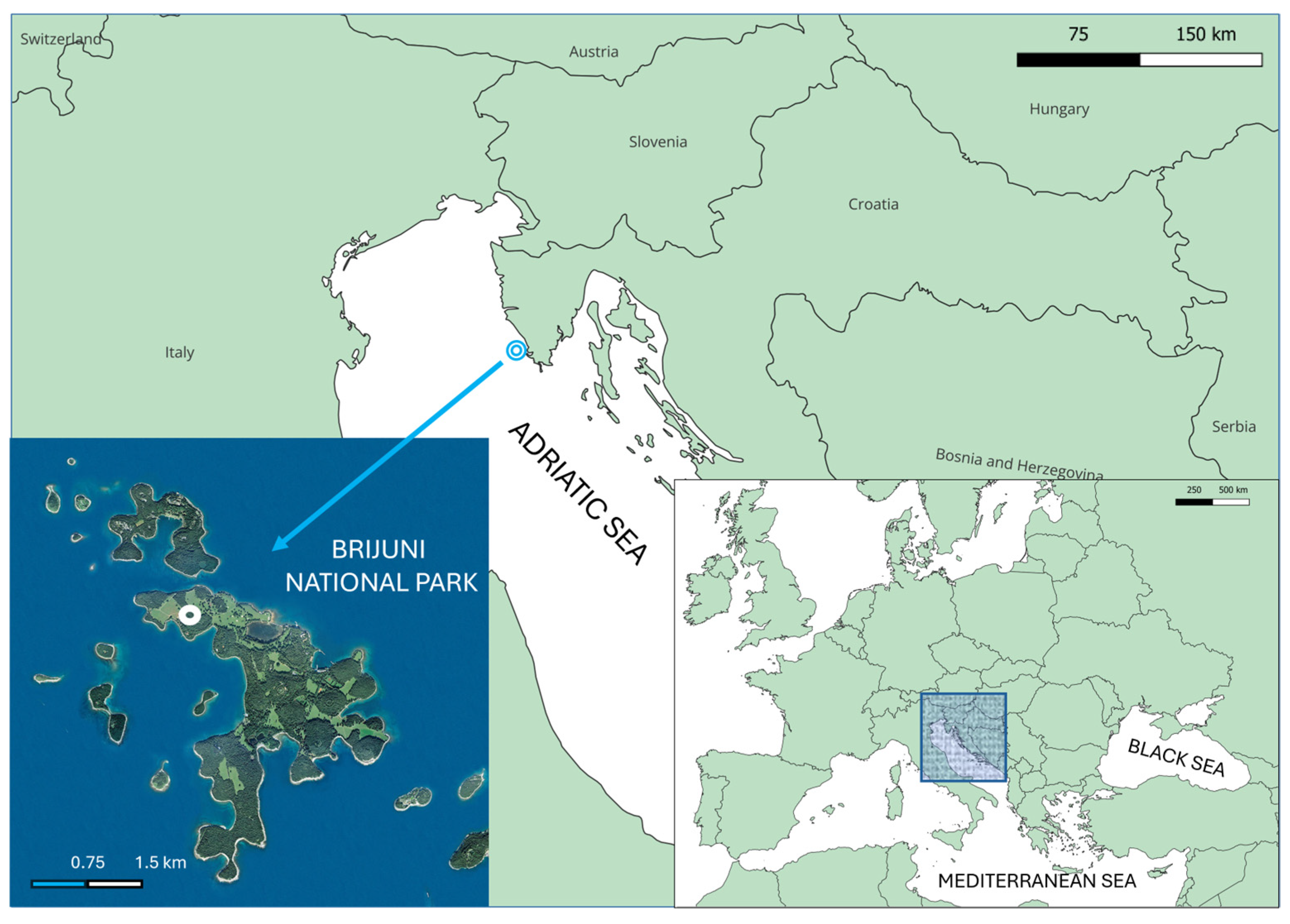
The Brijuni National Park area has distinctive geomorphological, hydrological, climatic, and landscape characteristics, with rich flora [29]. The total area of the park is 33.95 km², of which 7.43 km² represents the land area comprising 14 islands, with Veliki Brijun and Mali Brijun being the largest islands (Figure 1). The vegetation of the Brijuni archipelago is rich and diverse, shaping a unique landscape on the Croatian Adriatic coast [30]. Landscaped parks with large open grasslands occupy about two-fifths of the surface of the largest island, Veliki Brijun, while smaller park areas are also present on Mali Brijun. The dominant forest associations include the holm oak and manna ash community (Fraxino orni–Quercetum ilicis Horvatić (1956) 1958) with its subassociations typicum and lauretosum Horvatić 1958, as well as evergreen holm oak forests and maquis with myrtle (Myrto–Quercetum ilicis (Horvatić 1963) Trinajstić 1985) [31]. Among them, many species are anemophilous, such as the species characteristic of that area, Cupressus sempervirens L. (Italian cypress), meaning that wind disperses their pollen, which subsequently can represent an important source of organic matter in the atmosphere.

Atmospheric samples were collected in the northern part of the Veliki Brijuni area (Figure 1) between 4 October and 3 November 2021 as a representative autumn period characterized by frequent rainfall events. Rainwater samples were collected during six-day intervals, using six 1 L Duran^® glass bottles (Scherf Präzision Europa GmbH, Meiningen, Germany) installed in an automatic precipitation sampler (NSA 181—BASIC TYPE, Eigenbrodt GmbH & Co., Königsmoor, Germany), designed to exclusively collect precipitation while preventing the collection of dry deposition. The sampler consisted of a housing containing a funnel (collection area: 500 cm²), a polyethylene collection bottle, a lid, a precipitation sensor, and a heating unit (RS 85 sensor). During dry weather conditions, the funnel and collection bottle remained sealed by the lid. The lid automatically opened at the onset of precipitation and closed immediately after the precipitation event ended. This mechanism ensured that only precipitation scavenged from the atmosphere by wet deposition was collected, representing the fraction that would ultimately reach the ground via atmospheric washout. Prior to the sampling event, the funnel and all associated components were thoroughly cleaned using 10% hydrochloric acid (HCl; Merck-Millipore, Darmstadt, Germany) and subsequently rinsed with ultrapure Milli-Q water (MQ; 18.2 MW cm; Millipore, Billerica, MA, USA). In total, four rainwater samples (R1, R3, R4, R5) were collected during the sampling period, while no precipitation occurred during the sampling period 10–16 October 2021 (R2).

Bulk deposition samples were collected at six-day intervals using 2 L HDPE bottles (Thermo Electron LED GmbH, Langenselbold, Germany) mounted in a Bergerhoff collector (built in-house). All sampling bottles were pre-cleaned with 10% HCl and thoroughly rinsed with MQ water. During certain sampling intervals, when the wet deposition component was insufficient, a defined volume of MQ water was added to bulk deposition samples to dissolve the dry deposition fraction. A total of six bulk deposition samples (B1–B5) were collected during the study period, while one composite sample (B6) represents the entire sampling period (4 October–3 November 2021).

A total of 15 aerosol samples (A1–A15) were collected over a 2-day period each, using a low-volume automatic air sampler (PNS 18T-DM-3.1, Comde-Derenda, Stahnsdorf, Germany) equipped with a PM₁₀ inlet, enabling the collection of particles <10 µm in aerodynamic diameter. The air flow rate was 2.3 m³/h. Quartz fiber filters (d = 47 mm; Pall Life Sciences, Port Washington, NY, USA), pre-combusted at 450 °C for 4 h, were used for particle collection. Filters were weighed before and after sampling according to the standard gravimetric measurement method (EN 12341:2014) [32], and the mass difference corresponded to the collected particulate matter. The field blank filter without air passing through it was treated identically to the sampling filters. After sampling, all filters were placed in Petri slides and stored at −20 °C until analysis. The water-soluble aerosol fraction was prepared by immersing the filters in MQ water and leaching by ultrasonication in a water bath for 20 min, followed by extraction for 24 h at 4 °C.

The rainwater and bulk deposition samples, as well as aerosol extracts, were then syringe-filtered through 0.45 µm cellulose acetate membrane filters (Minisart, Sartorius, Göttingen, Germany), previously rinsed with MQ water, to separate the dissolved and particulate fractions. Two aliquots of dissolved samples were preserved with 10 mg/L HgCl₂ until dissolved organic carbon (DOC) and water-soluble dissolved organic carbon (WSOC) analysis, while all other analyses were done within 24 h after filtration. Prior to analysis, samples were diluted 2–4 times.

2.2. Meteorology and Air-Mass Backward Trajectories

An automatic meteorological station, the Davis Vantage Vue (Davis Instruments, Hayward, CA, USA) equipped with a USB data logger, was installed at a height of 2 m above ground level. The station is fitted with integrated sensors that enable continuous measurement and logging of key meteorological parameters, including air temperature, relative humidity, precipitation amount and intensity, as well as wind speed and direction.

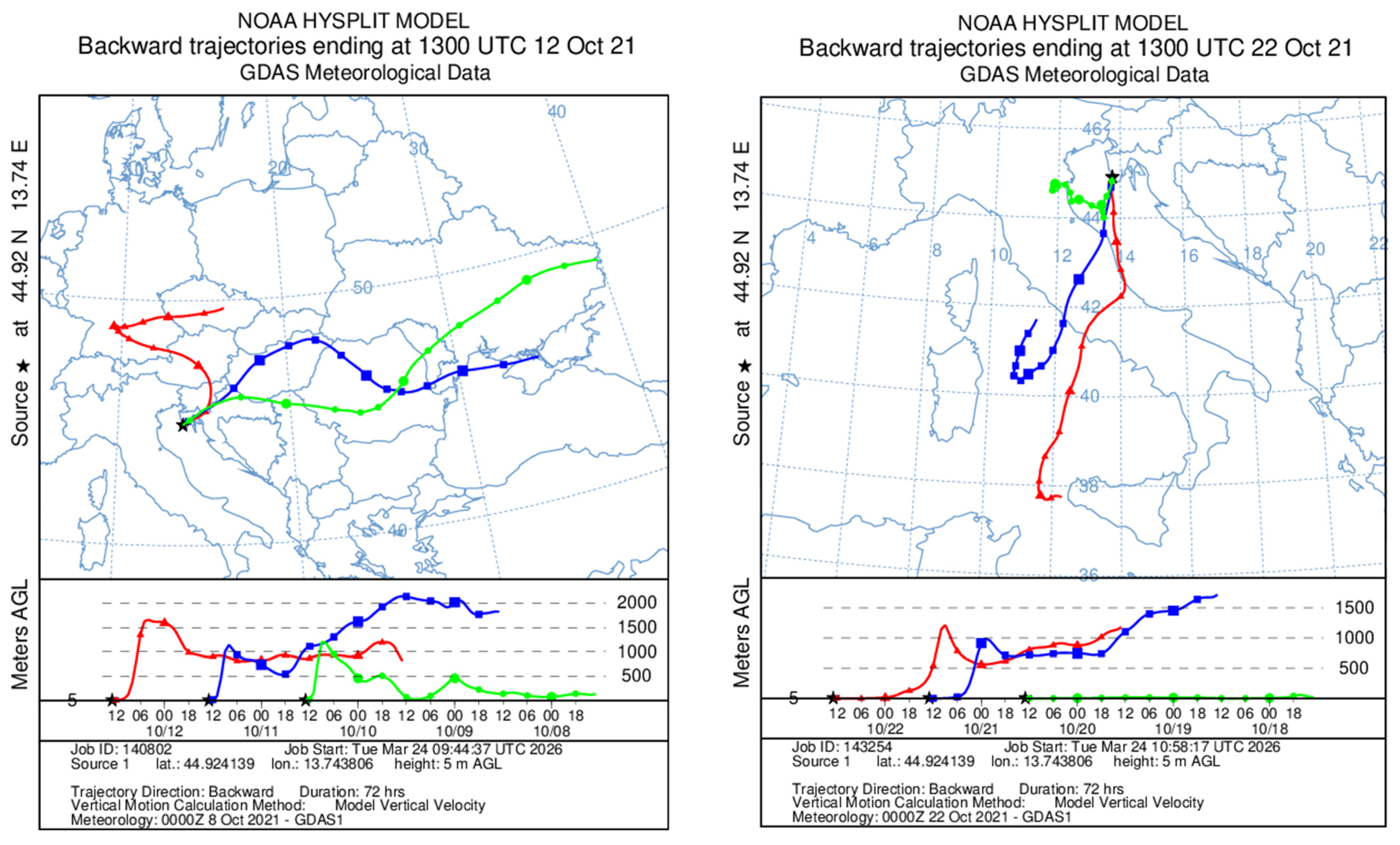
Air-mass backward trajectory analysis was conducted using the NOAA Hybrid Single-Particle Lagrangian Integrated Trajectory (HYSPLIT) model [33,34] driven by Global Data Assimilation System (GDAS; 1° global, 2006–present) meteorological data to distinguish dominant air mass sources and assess long-range transport. Fifteen 72 h backward trajectories were calculated at 24 h intervals, representing three characteristic time points within each 48 h sampling period (the start, midpoint, and end of sampling for each aerosol sample). Each plot shows an ensemble of three individual backward trajectories terminating at the Brijuni National Park at 5 m above ground level.

2.3. Chemicals, Solutions, and Model Material

MQ water was used throughout all experimental procedures, including solution preparation and cleaning of the electrodes and the electrochemical cell. All solutions were stored at 4 °C. The following chemicals were employed: sodium chloride (NaCl; Sigma-Aldrich, Steinheim, Germany) as a model electrolyte, prepared as a stock aqueous solution with a concentration of 5.5 M and further diluted; nitric acid (HNO₃, 65%, analytical grade, p.a., Kefo, Sisak, Croatia), prepared as a 10% (v/v) solution for cleaning the electrodes and the electrochemical cell; nitric acid (HNO₃, 65%, supra pure grade, s.p., Fisher Scientific, Loughborough, UK) for sample acidification; Triton-X-100 (T-X-100; t-Oct-C₆H₄-(OCH₂CH₂)_xOH, x = 9–10; Sigma-Aldrich, Steinheim, Germany), prepared as an aqueous solution with a concentration of 0.7 mg/L; copper(II) nitrate (Cu(NO₃)₂; Merck, Darmstadt, Germany), 1 g/L, prepared as 10⁻³ M solution and further diluted.

HULIS, previously isolated from marine aerosols by solid-phase extraction [35], was prepared at a stock concentration of 297.39 mg C/L (HULIS-C). Fulvic acid, isolated from river water (Suwannee River Fulvic Acid, SRFA; 3S101F: Suwannee River III), obtained from the International Humic Substances Society (IHSS; St. Paul, MN, USA), was prepared as a stock solution with a concentration of 100 mg/L. Both solutions were further diluted.

Cupressus sempervirens pollen, used as a source of atmospheric organic matter representative of the Brijuni area (a national park where the collection of plants and their parts is forbidden), was collected at the Botanical Garden of the Faculty of Science, University of Zagreb, during the pollination season. Pollen was obtained directly from the plants by harvesting mature anthers, which were subsequently ground and sieved through 125 μm and 20 μm meshes. The former removed larger debris such as anther fragments and plant tissue, while the latter retained purified pollen grains and excluded finer particulate impurities. The collected pollen samples were air-dried at room temperature for 24 h and stored at −20 °C until further use. A 40 mg/L suspension of two-week-old Cupressus pollen was prepared in MQ water, sonicated for 5 min and extracted at −4 °C for 24 h during which pollen grains ruptured and organic sub-pollen material was released. Prior to analysis, this suspension was filtered through 0.45 µm cellulose acetate membrane filters (Minisart, Sartorius, Göttingen, Germany), previously rinsed with MQ water.

2.4. Instruments and Methods

Electrochemical measurements were performed using a µAUTOLAB Type II potentiostat/galvanostat connected to a 663VA Stand three-electrode system (Metrohm, Herisau, Switzerland) and an IME (Interface for Mercury Electrode) unit. The system was controlled via a PC equipped with GPES 4.9 software. The 663VA Stand three-electrode system consists of three electrodes immersed in an electroanalytical cell: the working electrode was a hanging mercury drop electrode with a surface area of 0.52 mm², the reference electrode was an Ag/AgCl (3 M KCl), and the auxiliary electrode was a glassy carbon rod completing the circuit with the working electrode. All measured potentials are reported versus the reference electrode. A Teflon stirrer and a nitrogen gas inlet were also immersed in the electroanalytical cell. The cell was made of borosilicate glass, and the lid featured a septum through which standard solutions were added to the cell.

The electrochemical measurements were performed using DPASV and alternating current voltammetry (ACV). DPASV was used in complexometric titrations mandatory for the determination of CuCC in atmospheric deposition samples. The DPASV parameters were: nitrogen purging time of 300 s, accumulation potential E_a = −0.6 V, accumulation time t_a = 120 s, equilibration time t_eq = 10 s, step potential E_s = 4 mV, and amplitude a = 25 mV (if not stated otherwise). The ACV was employed to determine the maximum surface coverage (θ) of the working electrode in HULIS, SRFA, and pollen solution, as well as for the quantification of SAS in rainwater, bulk deposition samples, and the water-soluble aerosol fraction. The ACV measurements were conducted with the following parameters: E_a = −0.6 V, t_a = 60 s, t_eq = 10 s, frequency f = 77.35 Hz, phase angle φ = 90°, E_s = 40 mV, and a = 25 mV, if not stated otherwise.

During the experimental work, an analytical balance (XS205, Mettler-Toledo, Greifensee, Switzerland), an ultrasonic bath, and a homemade 150 W high-pressure mercury UV lamp were used. The pH of collected samples was measured using a digital pH meter (Hanna Instruments, Zagreb, Croatia) equipped with a microelectrode. The instrument was calibrated with standard buffer solutions of pH 4.00 and 7.00 (Kemika, Zagreb, Croatia) prior to measurement.

2.5. Determination of Dissolved/Water-Soluble Organic Carbon (DOC/WSOC)

Dissolved organic carbon in rainwater and bulk deposition samples, WSOC in aerosol extracts and organic carbon in HULIS solution (HULIS-C) were determined following the EN 1484:2002 standard [36] in a laboratory accredited according to HRN EN ISO/IEC 17025:2017 [37]. Measurements were performed using a TOC-V_CPH analyser (Shimadzu, Kyoto, Japan) with a platinum silica catalyst and nondispersive infrared (NDIR) detector that detects CO₂ after high-temperature catalytic oxidation (680 °C) of organic compounds. The concentration of organic carbon was calculated as an average of two replicate samples. Results are reported as the mean concentration of the two aliquots. The limit of detection was 0.03 mg/L.

2.6. Determination of Surface-Active Substances (SAS)

The ACV with out-of-phase mode (phase angle 90°) was used to determine SAS in the atmospheric samples with 0.55 M NaCl serving as the supporting electrolyte. A decrease in the capacitive current due to the adsorption of SAS on the working electrode surface was measured [27,35]. SAS concentration was expressed as the equivalent concentration of the HULIS-C as a model for atmospheric SAS [35], according to its calibration line (Δi_c = 0.6012 × γ(HULIS-C)). The limit of detection was 0.02 mg/L.

2.7. Determination of Copper Complexing Capacity (CuCC) Parameters

The CuCC represents the ability of organic matter in natural aquatic samples to “mask” a certain concentration of Cu²⁺ by binding it into inert complexes. In complexometric titrations, an aliquot of the sample at natural pH was titrated with standard Cu²⁺ solutions, allowing voltammetric detection of free/labile Cu²⁺. Prior to titration, high-purity nitrogen (5.0; Messer, Zagreb, Croatia) was purged through the sample in the electrochemical cell for 15 min to remove dissolved oxygen and facilitate Cu²⁺ complexation. DPASV results were presented as complexometric curves, showing the reoxidation peak current (i_p) as a function of total Cu²⁺ concentration in the sample (added plus naturally present). Mathematical modeling (Section 2.8) yielded the Cu-binding ligand concentration (i.e., CuCC) and the conditional stability constant (log K_i). Organic ligands with different Cu-binding strengths contribute to CuCC and, according to the “discrete model,” are classified into classes based on similar affinities of Cu-binding functional groups [38]. Consequently, CuCC generally does not provide structural information on specific ligands or complexes; instead, it is defined by the concentrations of organic ligand classes (L_i) and their corresponding conditional stability constants (K_i) [39]. The replicate analyses of independent samples were not possible due to limited sample volumes, though the relative standard deviation of the mean value calculated from five independent CuCC measurements by the DPASV method in rainwater is typically below 10% [40].

To determine the total dissolved Cu²⁺ concentration, a sample aliquot was acidified with HNO₃ (s.p., pH < 2) and exposed to UV radiation for 24 h to degrade organic ligands and release bound Cu²⁺. The sample was then titrated with a Cu²⁺ standard solution, measuring i_p as a function of added Cu²⁺ using the standard addition method. The accuracy of the DPASV method was verified using the certified reference material NASS-6 (Open Ocean Seawater Reference Material for Trace Metals, National Research Council of Canada). The measured dissolved Cu concentration was within 5% of the certified value.

2.8. Data Processing

The DPASV voltammograms were processed using ECDsoft software [41] to determine the peak current (i_p), peak potential (E_p), and half-peak width (w₁/₂). The total dissolved Cu²⁺ concentrations in samples were calculated using StandAdd software [42]. The complexometric titration data were mathematically transformed according to the Ružić–van den Berg, Scatchard, and Langmuir/Gerringa models incorporated in ProMCC software [43,44]. The Langmuir-Gerringa model enabled the determination of CuCC parameters ([L_i] and log K_i). The values are provided together with uncertainties computed by the fitting algorithm (fitter.dll) in the ProMCC and expressed as 95% confidence intervals. Based on the shape of the Scatchard plot, the number of ligand classes that bind Cu²⁺ (linear for one or nonlinear for two classes) in the samples was determined [43]. All graphs were generated using OriginPro 9.0. (OriginLab, Northampton, MA, USA).

2.9. Calculation of Fluxes

Deposition flux (F) represents the amount of a substance deposited per unit area over a given period. Wet (F_w) and bulk (F_b) deposition fluxes were calculated by multiplying the concentration of the substance in the sample (C) by the collected volume (V) and then dividing by the collection area (A) and the sampling duration (P):

F = (C × V)/(A × P)

Dry deposition fluxes (F_d) were estimated as F_d = C_d × V_d, where C_d is the concentration of water-soluble components in PM₁₀ (µg/m³), and V_d represents the deposition velocity (m/s). An approximate fine-to-coarse WSOC distribution ratio is 70:30 [45,46]. Accordingly, its deposition velocity (V_d) was estimated as V_d(WSOC) = f(fine) × V_d(fine) + f(coarse) × V_d(coarse), where f(fine) and f(coarse) represent the fractions of WSOC in fine and coarse particles, and V_d(fine) and V_d(coarse) are their respective deposition velocities. Based on this approach, a V_d value of 0.67 cm/s was obtained for WSOC. Deposition velocity for Cu²⁺ was 0.3 cm/s [10].

3. Results

3.1. Meteorological Conditions and Air-Mass Backward Trajectories

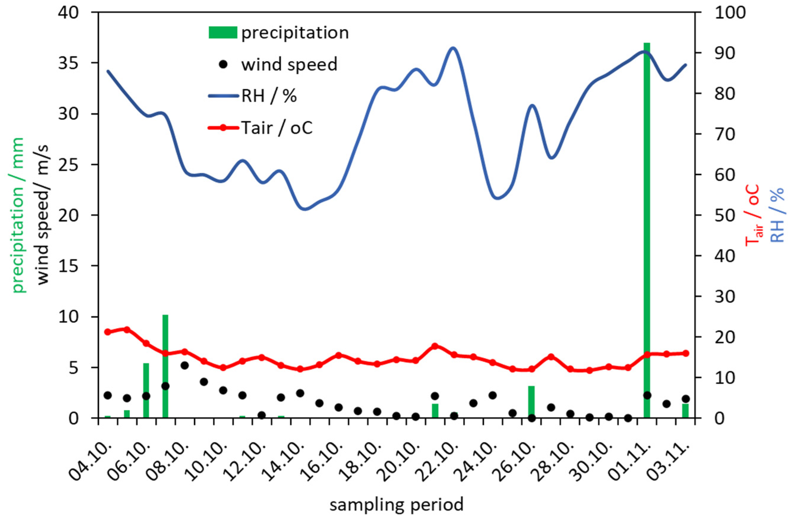
Figure 2 presents the temporal variation in precipitation amount, air temperature, wind speed, and relative humidity during the one-month period in the Brijuni National Park area. The minimum air temperature was recorded on 29 October 2021 (11.88 °C), while the maximum temperature occurred on 5 October 2021 (21.8 °C). Wind speeds ranged from 0.13 m/s (12 October 2021) to 5.2 m/s (8 October 2021). Total precipitation amounts varied between 0.2 and 37 mm per day. As shown in Figure 3, precipitation strongly influenced relative humidity, which was lower in the absence of rainfall and increased during precipitation events, ranging from 51.83% (14 October 2021) to 90.97% (22 October 2021).

The air mass origin affects atmospheric Cu complexation [20]. Therefore, we classified air masses that reached the Brijuni National Park area during the sampling period as continental (53%) and mixed air (continental and marine) masses (40%), which predominated (Figure 3), while the influence of purely marine air masses was minimal (7%).

3.2. Dissolved Organic Matter in Atmospheric Samples: DOC and SAS

Organic compounds present in atmospheric deposition samples could interfere with DPASV measurements by reducing sensitivity and potentially leading to distorted CuCC parameters. Therefore, we measured the concentration of WSOC and SAS in all deposition samples to study the SAS/WSOC proportion.

Table 1. Sampling dates, aerosol mass, m (mg), pH, water-soluble organic carbon, WSOC concentration (mg C/L), WSOC dry fluxes (F_d; mg/m² day), mass fraction of WSOC in aerosol (%), surface-active substances, SAS concentration (eq. mg HULIS-C/L), SAS mass in the air (µg C/m³), and SAS fraction (eq. HULIS-C) in WSOC (%) for aerosol samples (A) collected in the Brijuni National Park area in October–September 2021.

Sampling Period	Sample	m/mg	pH	γ(WSOC)/ mg C/L	Fd(WSOC)/ mg/m2 day	m(WSOC)/ m(Aerosol) %	γ(SAS)/eq. mg HULIS-C/L	γ(SAS)/ µg C/m3	m(SAS)/ m(WSOC) %
4–6 October	A1	1.51	6.27	3.854	0.4	5	1.139	0.21	30
6–8 October	A2	0.49	6.00	1.954	0.2	8	0.687	0.12	35
8–10 October	A3	0.55	5.46	6.246	0.6	23	1.817	0.33	29
10–12 October	A4	1.74	5.68	6.642	0.7	8	1.918	0.35	29
12–14 October	A5	0.45	5.91	3.742	0.4	17	1.587	0.29	42
14–16 October	A6	0.39	5.74	2.415	0.2	13	0.723	0.13	30
16–18 October	A7	0.73	5.51	6.386	0.7	17	1.918	0.35	30
18–20 October	A8	2.08	-	10.458	1.1	10	1.517	0.28	15
20–22 October	A9	1.68	5.97	7.15	0.7	9	1.817	0.33	25
22–24 October	A10	0.75	5.80	3.554	0.4	10	1.817	0.33	51
24–26 October	A11	0.87	6.29	5.334	0.5	12	1.587	0.29	30
26–28 October	A12	1.14	5.48	7.23	0.7	13	1.918	0.35	27
28–30 October	A13	1.97	5.00	11.218	1.1	11	2.040	0.37	18
30 October–1 November	A14	2.25	4.70	16.762	1.7	15	1.918	0.35	11
1–3 November	A15	1.33	5.87	3.326	0.4	5	1.587	0.29	48

presents the results of aerosol mass collected on filters over a one-month period in the Brijuni National Park area, together with pH, WSOC, and SAS values measured in the water-soluble aerosol fraction. The mass of collected aerosols ranged from 0.385 mg (A6) to 2.245 mg (A14), while the pH of the water-soluble fraction varied between 4.70 and 6.29. WSOC concentrations ranged from 1.954 to 16.762 mg C/L, and SAS concentrations from 0.687 to 2.040 eq. mg HULIS-C/L. The mass fraction of WSOC in the aerosol mass ranged from 5% (A1, A15) to 23% (A3), while the mass fraction of SAS in WSOC ranged from 11% (A14) to 51% (A10).

The collected rainwater volume, pH, DOC and SAS concentrations for five rainwater samples are presented in

Table 2. Sampling dates, volume collected, V (mL), pH, dissolved organic carbon, DOC concentration (mg C/L), DOC wet flux (F_w; mg/m² day), surface-active substances, SAS concentration (eq. mg HULIS-C/L), and SAS fraction in DOC (%) for rainwater (R) collected in the Brijuni National Park area in 2021.

Sampling Period	Sample	V/mL	pH	γ(DOC)/ mg C/L	Fw(DOC)/ mg/m2 day	γ(SAS)/eq. mg HULIS-C/L	m(SAS)/ m(DOC) %
4–10 October	R1	535	5.30	0.283	0.5	0.121	43
10–16 October	R2	0	-	-	-	-	-
16–22 October	R3	68.5	6.13	0.728	0.2	0.362	50
22–28 October	R4	110.5	5.96	0.346	0.1	0.063	18
28 October–3 November	R5	980	5.25	0.430	1.4	0.063	15

. No precipitation occurred during the sampling period 10–16 October 2021 (R2). During the remaining sampling intervals, collected rainwater volumes ranged from 68.5 to 980 mL, and pH values varied between 5.25 and 6.13. DOC concentrations ranged from 0.283 to 0.728 mg C/L, while SAS concentrations ranged from 0.063 to 0.362 eq. mg HULIS-C/L. The highest DOC and SAS concentrations were observed in sample R3 (16–22 October 2021). The contribution of SAS to the DOC pool ranged from 15% (R5) to 50% (R3).

Table 3. Sampling dates, volume collected, V (mL), pH, dissolved organic matter, DOC concentration (mg C/L), DOC total bulk flux (mg/m² day), surface-active substances, SAS concentration (eq. mg HULIS-C/L), and SAS fraction in DOC (%) for bulk (B) deposition samples collected in the Brijuni National Park area in 2021.

Sampling Period	Sample	V/mL	pH	γ(DOC)/ mg C/L	Fb(DOC)/ mg/m2 day	γ(SAS)/eq. mg HULIS-C/L	m(SAS)/ m(DOC) %
4–10 October	B1	100 1	6.28	1.325	3.6	0.286	22
10–16 October	B2	100 1	5.75	1.059	2.8	0.206	19
16–22 October	B3	100 1	5.70	0.986	2.6	0.206	21
22–28 October	B4	100 1	6.06	0.886	2.4	0.356	40
28 October–3 November	B5	193	5.59	0.633	3.3	0.356	56
4 October–3 November	B6	209.5	5.95	1.146	1.3	0.362	32

Note: ¹ MQ water added.

summarizes the collected volumes of bulk atmospheric deposition samples, the pH, and the concentrations of SAS and DOC for six bulk deposition samples. Due to the absence of wet deposition during the sampling period from 4 to 28 October 2021, MQ water was added to samples B1–B4 to dissolve the dry deposition component and enable further analyses. The amounts of wet deposition collected in the remaining samples ranged from 193 mL (B5) to 209.5 mL (B6). The pH values of the samples ranged from 5.70 (B3) to 6.28 (B1). DOC concentrations ranged from 0.633 mg C/L (B5) to 1.325 mg C/L (B1), while SAS concentrations varied between 0.206 eq. mg HULIS-C/L (B2, B3) and 0.356 eq. mg HULIS-C/L (B4, B5). The contribution of SAS to DOC in B1 to B5 ranged from 19% (B2) to 56% (B5), with an average of 32%, which completely reflected the result for the composite sample (32%, B6).

The SAS proportion of up to 51% in DOC of aerosols, up to 50% in rainwater, and up to 56% in bulk deposition suggested that the presence of SAS may cause interferences in complexometric titrations with Cu²⁺, and pointed to the next methodological step of studying adsorption properties of specific atmospheric SAS to define the procedures and DPASV measurement conditions for complexometric titrations aimed at minimizing their effect.

Estimated dry deposition WSOC fluxes (F_d) ranged from 0.2 to 1.7 mg/m² day, with an average value of 0.7 mg/m² day (Table 1). Wet deposition DOC fluxes (F_w) varied between 0.1 and 1.4 mg/m² day, with an average of 0.6 mg/m² day (Table 2). The relatively comparable magnitudes of dry and wet fluxes suggest that both mechanisms contributed significantly to organic carbon deposition, although their relative importance depended on meteorological conditions, particularly frequency and intensity of precipitation events. During the highest precipitations (6 October and 1 November 2021), dry deposition WSOC fluxes were the lowest and wet DOC deposition fluxes the highest. Bulk deposition DOC fluxes (F_b), calculated from weekly samples (B1–B5; Table 3), ranged from 2.4 to 3.6 mg/m² day, with an average of 2.9 mg/m² day. The composite sample (B6) yielded a flux value (1.3 mg/m² day) that is lower than the average of the B1–B5 samples, indicating that episodic high-deposition events were smoothed out over the longer sampling period, resulting in an underestimation of peak fluxes. On the other hand, composite bulk DOC flux reasonably reflected the overall (average dry + average wet) deposition over the studied period.

3.3. Voltammetry of Model SAS: Atmospheric HULIS, SRFA, and Pollen Organics

3.3.1. Surface-Active Properties

HULIS constitute a significant fraction of WSOC and are important components of atmospheric aerosols and cloud water, where they act as SAS [27,35]. As SRFA is structurally very similar to HULIS, we have studied the adsorption/desorption properties of both HULIS and SRFA on/from the hydrophobic surface of the working electrode. In this context, we also investigated specific atmospheric organic matter derived from airborne pollen of Cupressus sempervirens, a characteristic plant of the Brijuni area.

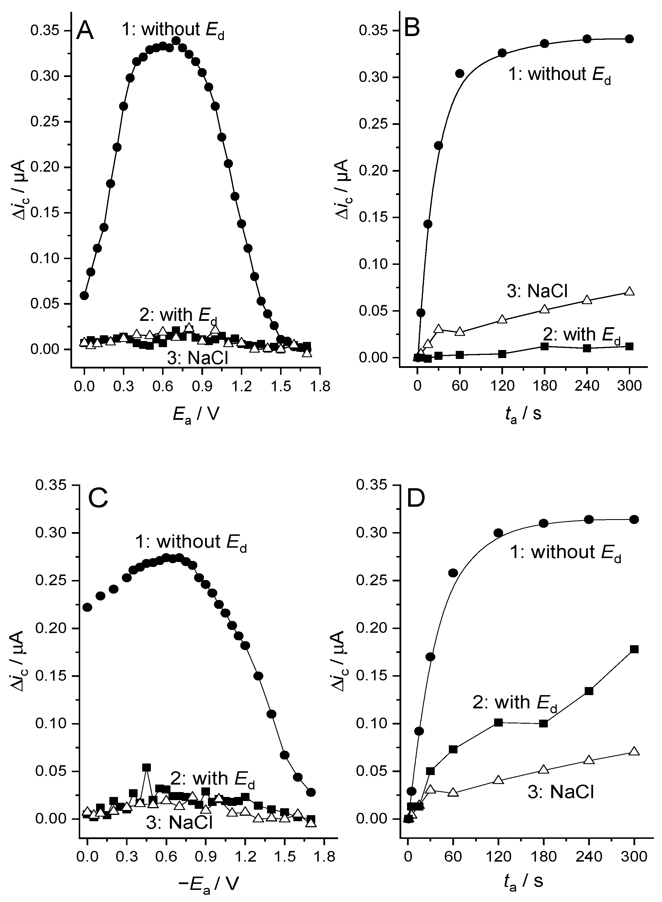
The difference in ACV capacitive currents (ΔI_c) recorded at individual accumulation potentials (E_a) (in relation to the current at the most negative accumulation potential applied, −1.7 V) in HULIS and pollen solutions is shown in Figure 4A and Figure 4C, respectively. For curve 1, different E_a values were applied during an accumulation time of 60 s, whereas for curve 2, an additional desorption step was applied at the end of the accumulation period. The ΔI_c response obtained in the model electrolyte (0.55 M NaCl) without application of a desorption step is shown as curve 3. Maximum HULIS and pollen organic material adsorption on the electrode surface occurred around E_a = −0.6 V, where the hydrophobic mercury surface carries no charge. As E_a was shifted towards more negative values, the surface became negatively charged, which resulted in a gradual decrease in adsorption (curve 1). Application of the desorption step (E_d = −1.7 V for 1 s) after accumulation removed nearly the entire adsorbed HULIS and pollen material layer from the electrode surface (curves 2), yielding a response comparable to that of the model electrolyte lacking organic matter (curves 3). Figure 4B,D show the dependence of ΔI_c on the accumulation time (t_a). The degree of surface coverage achieved after 1 s at −0.6 V without a desorption step (curve 1) corresponded to that obtained after 120 s of accumulation without a desorption step, demonstrating the high efficiency of HULIS desorption from the mercury electrode at negative potentials. Very similar results were observed for SRFA (Figure S1): the degree of surface coverage achieved after 5 s at −0.6 V without a desorption step (curve 1) was comparable to that obtained after 240 s of accumulation when the desorption step was applied (curve 2; Figure S1B). These results suggest that the application of a highly negative desorption potential resulted in the removal of the adsorbed organic layer from the electrode surface.

3.3.2. Interferences in CuCC Determination

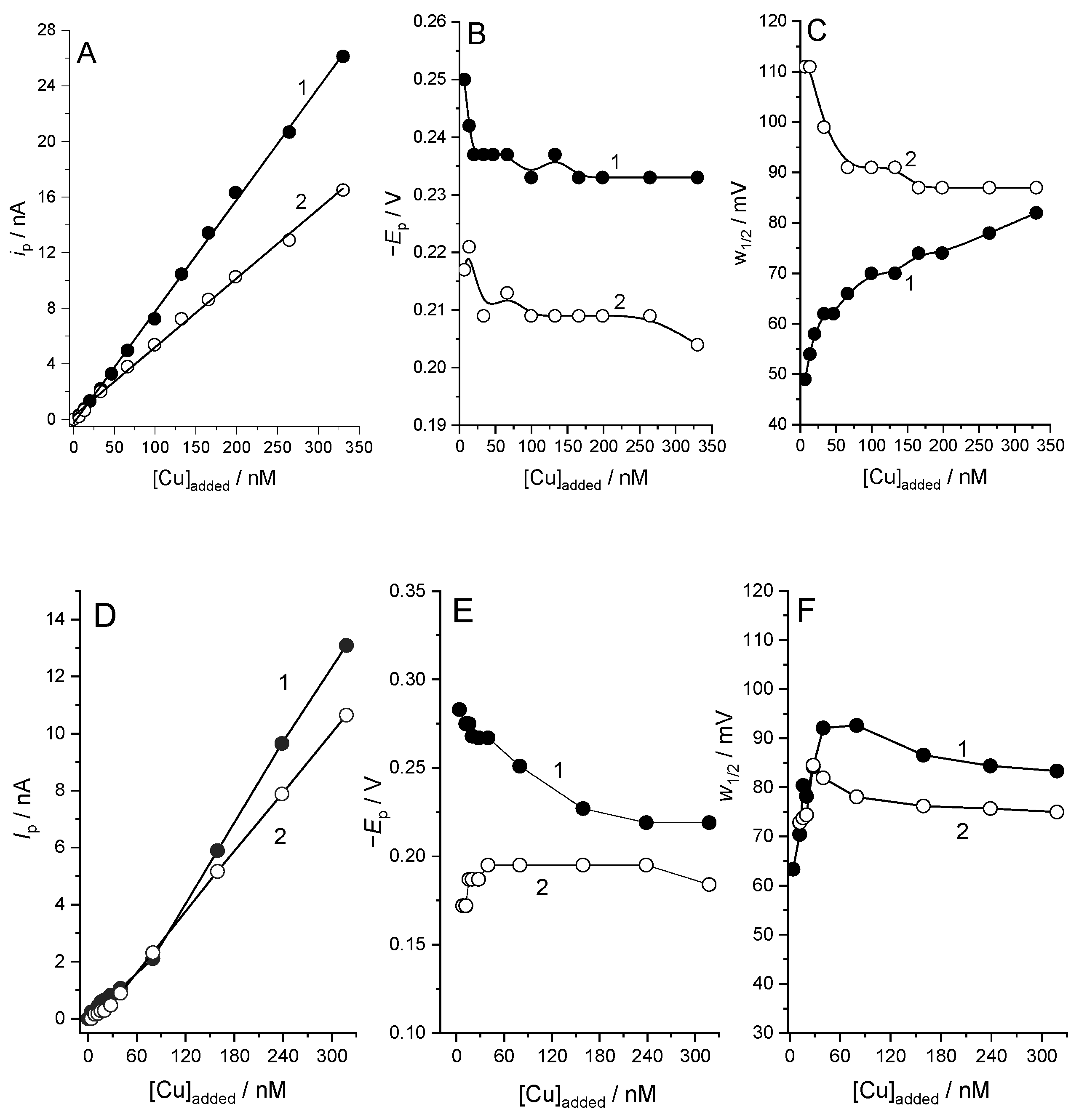
Considering the desorption properties of HULIS, SRFA and pollen organics at highly negative potentials (as shown in Section 3.3.1), their influence on Cu redox behavior in the solution of HULIS, SRFA and pollen was investigated using the DPASV method. In the range of desorption potentials (E_d) from −0.6 to −1.7 V applied for 1 s, potentials more negative than −1.4 V, −1.5 V and −0.8 V for SRFA, pollen, and HULIS, respectively, yielded a maximum reoxidation peak of 100 nM Cu²⁺. Furthermore, in the range of 0.1 to 7 mg/L T-X-100, an increase in the peak current (i_p) was observed up to 0.5, 1 and 1 mg/L of HULIS, SRFA, and pollen solution, respectively, beyond which further increases in T-X-100 concentration did not affect i_p. Taking into account the beneficial effects of both factors, two complexometric titrations were further performed in a solution of 1 mg/L HULIS-C, 36 mg/L Cupressus sempervirens (Figure 5), and in 1 mg/L SRFA (Figure S2), one applying E_d = −1.0 V (HULIS), −1.4 V (SRFA) and −1.7 V (Cupressus) for 1 s and adding 1 mg/L T-X-100, and the other without the E_d and T-X-100.

The application of a desorption step and the addition of model T-X-100 significantly improved the voltammetric response of Cu²⁺ in both solution (Figure 5). Under these conditions, the Cu reoxidation peak was higher, shifted toward more negative potentials and became narrower (lower w_1/2), indicating energetically facilitated reoxidation and a well-shaped peak. In contrast, in the absence of E_d and T-X-100, adsorbed HULIS probably hindered the redox process on the working electrode, resulting in broader peaks and less negative peak potentials, indicating energetically less favorable reoxidation. A similar behavior was observed for SRFA (Figure S2), where the application of E_d and T-X-100 also resulted in enhanced peak definition, leading to higher sensitivity. Similar results in terms of peak current and peak potential were also obtained in the pollen solution (Figure 5D,E), while a difference was observed in w_1/2, which was less pronounced compared to HULIS and SRFA (Figure 5F). These results suggested that application of relatively negative E_d for 1 s and addition of 1 mg/L T-X-100 in atmospheric deposition samples would be mandatory for accurate CuCC determinations in atmospheric deposition samples. Therefore, all deposition samples were measured at conditions of E_d = −1.4 V and 1 mg/L T-X-100.

3.4. CuCC in Different Types of Atmospheric Samples

The concentration of Cu²⁺ in aerosols from the Brijuni area ranged from 0.20 to 2.57 ng/m³ (

Table 4. Sampling dates, total Cu²⁺ concentration in air (ng/m³), dry Cu²⁺ fluxes (F_d, µg/m² day), copper complexing capacity, CuCC parameters (total organic ligand concentration, [L] and conditional stability constant, log K) for water-soluble aerosol fraction samples (A) collected in the Brijuni National Park area.

Sampling Period	Sample	γ(Cu2+)/ ng/m3	Fd(Cu2+)/ µg/m2 day	[L]/nM	log K
4–6 October	A1	2.21	0.6	139.8 ± 9.4	8.9 ± 0.3
6–8 October	A2	0.20	0.1	173.2 ± 4.4	11.2 ± 0.7
8–10 October	A3	0.75	0.2	96.6 ± 3.3	9.7 ± 0.7
10–12 October	A4	0.53	0.1	202.4 ± 12.6	10.8 ± 0.3
12–14 October	A5	1.18	0.3	176.4 ± 4.4	11.4 ± 0.7
14–16 October	A6	0.43	0.1	69.6 ± 3.3	10.7 ± 0.7
16–18 October	A7	2.06	0.5	183.6 ± 4.4	10.4 ± 0.7
18–20 October	A8	1.96	0.5	214.5 ± 3.3	9.8 ± 0.7
20–22 October	A9	2.57	0.7	392 ± 4.4	9.3 ± 0.7
22–24 October	A10	0.90	0.2	369.6 ± 4.4	9.8 ± 0.7
24–26 October	A11	0.51	0.1	296.8 ± 4.4	10.4 ± 0.7
26–28 October	A12	0.93	0.2	221.2 ± 4.4	10.2 ± 0.3
28–30 October	A13	1.61	0.4	212.0 ± 12.6	10.2 ± 0.3
30 October–1 November	A14	2.05	0.5	270.0 ± 12.6	10.0 ± 0.3
1–3 November	A15	0.74	0.2	130.0 ± 12.6	10.3 ± 0.3

), with an average of 1.24 ng/m³. This is consistent with background Cu²⁺ concentrations measured in PM₁₀ samples during the February-July period in the central Adriatic coastal area (1.99 ± 1.72 ng/m³) [10]. It indicates that our study area was not under the pressure of atmospheric sources of Cu during the investigation period. However, the dry Cu²⁺ flux was in the range 0.1–0.7 µg/m² day (Table 4) and the wet Cu²⁺ flux ranged from (0.2 ± 0.0) to (1.6 ± 0.1) µg/m² day (

Table 5. Sampling dates, total Cu²⁺ concentration, wet Cu²⁺ flux (F_w; µg/m² day), copper complexing capacity, CuCC (expressed as ligand concentration [L]), and conditional stability constant, log K for rainwater (R) samples collected in the Brijuni National Park area in October–November 2021.

Sampling Period	Sample	[Cu2+]/nM	Fw(Cu2+)/ µg/m2 day	[L]/nM	log K
4–10 October	R1	7.2 ± 0.5	0.8 ± 0.1	51.5 ± 5.7	10.06 ± 0.20
10–16 October	R2	-	-	-	-
16–22 October	R3	17.7 ± 0.9	0.3 ± 0.0	306 ± 5.7	9.91 ± 0.20
22–28 October	R4	7.8 ± 0.4	0.2 ± 0.0	58.5 ± 5.7	9.79 ± 0.20
28 October–3 November	R5	7.8 ± 0.6	1.6 ± 0.1	52.2 ± 3.1	8.22 ± 0.27

). The bulk Cu²⁺ flux ranged from (1.2 ± 0.1) to (2.4 ± 0.1) µg/m² day (average of (1.9 ± 0.1) µg/m² day) (

Table 6. Sampling dates, total Cu²⁺ concentration, bulk Cu²⁺ flux (F_b; µg/m² day), copper complexing capacity, CuCC (i.e., ligand concentration [L]), and conditional stability constant, log K for bulk (B) deposition samples collected in the Brijuni National Park area in October–November 2021.

Sampling Period	Sample	[Cu2+]/nM	Fb(Cu2+)/ µg/m2/d	[L]/nM	log K
4–10 October	B1	10.1 ± 0.5	1.7 ± 0.1	263 ± 5.7	10.55 ± 0.20
10–16 October	B2	13.5 ± 0.9	2.3 ± 0.2	262 ± 5.7	10.47 ± 0.20
16–22 October	B3	7.05 ± 0.5	1.2 ± 0.1	68.0 ± 3.1	8.99 ± 0.27
22–28 October	B4	13.8 ± 0.5	2.4 ± 0.1	94.4 ± 3.1	10.06 ± 0.27
28 October–3 November	B5	6.15 ± 0.3	2.0 ± 0.1	27.7 ± 2.8	9.15 ± 0.92
4 October–3 November	B6	15.4 ± 0.5	1.1 ± 0.0	157 ± 3.1	10.72 ± 0.27

). This is in the range of the bulk Cu²⁺ fluxes calculated for the central Adriatic coastal area (2019), which were in the range 1.2–10.8 (average (4.2 ± 3.1) µg/m² day) [10], but significantly lower than the value (30.9 ± 5.7) µg/m² day obtained for the Venice area (northern Adriatic, 1993–1997) [47].

The water-soluble aerosol fraction exhibited relatively high Cu-binding organic ligand concentrations ranging from (69.6 ± 3.3) nM (A6) to (392 ± 4.4) nM (A10). The conditional stability constants of the formed Cu²⁺ complexes ranged from log K = (8.9 ± 0.3) (A1) to log K = (11.4 ± 0.7) (A5; Table 4).

In rainwater samples, the calculated ligand concentration ranged from (51.5 ± 5.7) to (306 ± 5.7) nM with log K = (8.22 ± 0.27)–(10.06 ± 0.20) (Table 5). The highest total Cu²⁺ concentration was determined in sample R3, (17.7 ± 0.9) nM, while the lowest total Cu²⁺ concentration was observed in sample R1, (7.24 ± 0.46) nM.

In bulk deposition samples, ligand concentrations ranged from (27.7 ± 2.8) nM (B5) to (263 ± 5.7) nM (B1) (Table 6). The determined log K values varied between (8.99 ± 0.27) (B3) and (10.72 ± 0.27) (B6).

4. Discussion

The DPASV detection of Cu²⁺ in aquatic systems is strongly influenced by the adsorbed layer of natural organic matter on the working electrode surface [22,28,48]. Previous studies have shown that the addition of non-ionic surfactant T-X-100 to natural water samples, such as the estuary [28] and the sea surface microlayer [22] samples with high organic carbon content (up to 5.2 mg C/L and up to 6.8 mg C/L, respectively) enhance Cu sensitivity, thereby facilitating the reliable determination of CuCC [28]. T-X-100, a model SAS, does not interfere with Cu redox processes, but competitively diminishes the adsorption of present organic matter on the working electrode surface, facilitating Cu reoxidation [28,49]. Surface-active substances constituted up to 56% of DOC in atmospheric inputs from the Brijuni National Park, making them a significant interference in DPASV measurements of CuCC. The applied methodological approach, including the desorption step (E_d = −1.4 V) and the addition of T-X-100, proved essential for the reliable determination of CuCC parameters in atmospheric samples with a high amount of SAS. Their removal or suppression enabled better-defined voltammetric signals, reflected in sharper peaks and higher current responses. This confirmed that method optimization is a critical step when applying voltammetric techniques to complex atmospheric matrices, in addition to previous studies in estuarine and seawater samples.

Atmospheric deposition represents an important pathway for the transport of trace metals and organic matter from the atmosphere to the marine environments [10,50,51]. Although the number of atmospheric samples in our study is limited, consistent differences in CuCC concentrations were observed among sample types. The highest average CuCC values were found in the water-soluble aerosol fraction ((209.8 ± 6.7) nM), followed by bulk deposition ((142.9 ± 4.1) nM), and rainwater ((117.1 ± 5.0) nM), indicating variability in ligand abundance across atmospheric inputs. In contrast, the average conditional stability constants were similar among all sample types (log K = 9.6–10.2), suggesting that comparable types of organic ligands are responsible for Cu complexation in these matrices. Therefore, the observed differences in CuCC are primarily related to variations in ligand concentration rather than ligand strength, reflecting differences in the amount of organic matter present in each type of atmospheric sample.

Based on the linear shape of the Scatchard plot [43], one class of Cu-binding ligands was identified in all atmospheric samples. The relatively high ligand concentrations ([L] = 27.7–392 nM) and relatively low stability constants (log K = 8.22–11.40) indicate that these atmospheric systems were dominated by a weaker ligand class (L₂). This behavior differs from marine systems, where multiple ligand classes are typically present, including both stronger (L₁; log K > 12) and weaker (L₂; log K < 12) ligands [15,22,28]. Strong Cu-binding ligands in seawater are typically of biological origin, produced by phytoplankton and bacteria, whereas weaker ligands are mainly associated with bulk dissolved organic matter, including humic substances and terrestrially derived inputs, as well as degraded ligands and resuspended benthic inputs [15,52,53,54]. Accordingly, atmospheric inputs directly contributed to the weaker organic ligand pool in the studied coastal marine areas. The DPASV detection of a weaker ligand class in atmospheric deposition suggests a distinct origin and composition of organic matter compared to marine dissolved organic matter. The atmospheric organic matter is enriched in low-molecular-weight and partially oxidized organic ligands [18]. To this group also fits HULIS, commonly found in atmospheric aerosols, that exhibit surface-active properties and moderate metal-binding capacity [55]. Furthermore, the inclusion of pollen-derived organic material highlighted the potential contribution of terrestrial biogenic sources to atmospheric CuCC in the studied area. Anemophilous plant species, such as Cupressus sempervirens, are abundant in the study area and release pollen into the atmosphere. The sub-pollen organic matter can contribute organic ligands capable of interacting with trace metals, representing an additional and previously underexplored source of Cu-binding compounds [22,56]. Moreover, specific airborne pollen organic material makes weak Cu complexes (log K = 9.5–9.9) [22]. However, it should be noted that voltammetric ligand characterization is inherently method-dependent. Therefore, the identification of a single class of relatively weak ligands reflects the applied DPASV experimental conditions and detection window and does not necessarily exclude the presence of stronger ligand classes in atmospheric inputs.

In rainwater samples, CuCC values were ((51.5 ± 5.65) to (306 ± 5.65) nM), well above total Cu²⁺ concentrations ((7.24 ± 0.46) to (17.7 ± 0.85) nM), indicating that Cu was fully complexed, as previously reported for coastal [17] and semi-urban rainwater [5]. A comparable trend was also observed in bulk deposition samples, where CuCC values ((27.7 ± 2.77) to (263 ± 5.65) nM) exceeded total Cu²⁺ concentrations ((6.15 ± 0.26) to (15.4 ± 0.50) nM). Accordingly, this could affect the availability of Cu²⁺ in interfacial processes and heterogeneous chemical reactions in the atmosphere [2], and Cu chemical speciation and its biological effect in seawater upon input [8]. The obtained conditional stability constants of Cu-organic matter complexes in rainwater are within a range of constants previously reported for urban and coastal rainwater in nearby areas, log K = 6.1–10, together with one identified weak ligand class, determined with the same method of DPASV [23]. The conditional stability constants determined with adsorptive cathodic stripping voltammetry with tropolone as an artificial competing ligand added are reported to be higher, log K = 11–14 [5,19], while log K = 13–16 was reported if salicylaldoxime was used [17]. In addition, in these reports, strong and weak ligand classes were identified. The evident differences are due to different methods (DPASV versus adsorptive cathodic stripping voltammetry) or different competing ligands used in complexometric titrations that offer different detection windows, i.e., detect complexes of different ranges of stability, as discussed in [5,17]. Finally, the obtained stability constants should be interpreted as conditional values valid under the physicochemical conditions of the samples and applied experimental conditions of the DPASV method, optimized in a way to reduce analytical artifacts due to SAS, thereby fully preserving the original speciation in samples.

The comparison of dry, wet, and bulk deposition fluxes of DOC revealed that bulk deposition integrates contributions from both processes, resulting in higher overall fluxes. However, variability between individual samples reflects changing meteorological conditions and air mass origins, being continental and mixed continental and marine, which are known to influence both the concentration and composition of atmospheric organic matter [57]. The lower flux observed in the composite bulk sample (F_b(DOC) = 1.3 mg/m² day) compared to the average of weekly bulk samples (F_b(DOC) = 2.9 mg/m² day) suggests that episodic high-deposition events are smoothed over longer sampling periods. The DOC average bulk deposition flux observed in Brijuni National Park (2.9 mg/m² day) is comparable to the value of 1.9 mg/m² day reported for the northwestern Mediterranean (Frioul Island) [58]. Lower WSOC dry deposition fluxes of 0.7 mg/m² day in the Brijuni area are also comparable with 0.5 mg/m² day estimated for the eastern Mediterranean (Finokalia) [59]. Regarding DOC wet deposition fluxes, in comparison to 0.6 mg/m² day in the Brijuni area, significantly higher values have been reported in more anthropogenically influenced regions, such as urban areas in China (7.9 mg/m² day) [60] and Jiaozhou Bay (8.6 mg/m² day) [61], where stronger emission sources and higher atmospheric pollutant loads contribute to enhanced organic carbon deposition. These comparisons suggest that the Brijuni site represents a moderately impacted coastal area in the northern Mediterranean, with WSOC fluxes characteristic of Mediterranean background conditions but still sensitive to episodic atmospheric inputs.

It should be noted that this study is based on a short-term sampling campaign and, therefore, may not capture seasonal variability in atmospheric inputs. Previous studies have shown that both the quantity and chemical composition of atmospheric organic matter can vary significantly with season, driven by biological activity, photochemical processes, and different emission sources [10,62,63]. Consequently, the presented results should be interpreted as representative of short-term conditions and serve as background for long-term investigations, providing preliminary data necessary for the design of sampling frequency and optimization of extended study programs. Such an approach is particularly relevant in protected areas, where ecosystems are especially sensitive and susceptible to atmospheric inputs. Understanding the nature and variability of different atmospheric inputs is therefore essential for predicting trace metal cycling at the atmosphere–ocean interface.

5. Conclusions

This study demonstrates for the first time that reliable determination of CuCC in atmospheric samples requires careful optimization of voltammetric conditions, particularly due to the presence of SAS. The application of a desorption step and T-X-100 significantly improved analytical performance, enabling robust characterization of Cu-binding ligands. The voltammetric results obtained for the Brijuni area are method-specific and show that atmospheric inputs to the coastal marine environment are dominated by relatively weak Cu-binding ligands, with Cu predominantly present in a complexed form in rainwater and bulk deposition samples. Short-term monitoring revealed variability in atmospheric inputs and highlighted the role of organic matter composition, including biogenic contributions such as pollen. Overall, atmospheric deposition represents an important pathway for the input of organic ligands influencing Cu speciation in the studied coastal marine system. However, as the study is limited to a short autumn sampling period, the results may not fully capture seasonal variability in the atmospheric composition of organic matter, including changes in biological inputs, photochemical processing, and deposition pathways. Therefore, the findings should be interpreted as representative of the investigated period, providing a methodological and conceptual basis for further long-term studies needed to better constrain seasonal dynamics and the overall impact of atmospheric inputs on Cu speciation in the coastal marine environment of the northern Mediterranean.

References

1. Galloway, J.N.; Thornton, J.D.; Norton, S.A.; Volchok, H.L.; Mclean, R.A.N. Trace-Metals in Atmospheric Deposition: A Review and Assessment. Atmos. Environ. 1982, 16, 1677–1700. [Google Scholar] [CrossRef]
2. Deguillaume, L.; Leriche, M.; Desboeufs, K.; Mailhot, G.; George, C.; Chaumerliac, N. Transition metals in atmospheric liquid phases: Sources, reactivity, and sensitive parameters. Chem. Rev. 2005, 105, 3388–3431. [Google Scholar] [CrossRef] [PubMed]
3. Kieber, R.J.; Skrabal, S.A.; Smith, C.; Willey, J.D. Redox speciation of copper in rainwater: Temporal variability and atmospheric deposition. Environ. Sci. Technol. 2004, 38, 3587–3594. [Google Scholar] [CrossRef]
4. Lin, M.F.; Yu, J.Z. Assessment of Interactions between Transition Metals and Atmospheric Organics: Ascorbic Acid Depletion and Hydroxyl Radical Formation in Organic-Metal Mixtures. Environ. Sci. Technol. 2020, 54, 1431–1442. [Google Scholar] [CrossRef]
5. Spokes, L.J.; Lucia, M.; Campos, A.M.; Jickells, T.D. The role of organic matter in controlling copper speciation in precipitation. Atmos. Environ. 1996, 30, 3959–3966. [Google Scholar] [CrossRef]
6. Nriagu, J.O. A Global Assessment of Natural Sources of Atmospheric Trace-Metals. Nature 1989, 338, 47–49. [Google Scholar] [CrossRef]
7. Duce, R.A.; Liss, P.S.; Merrill, J.T.; Atlas, E.L.; Buat-Menard, P.; Hicks, B.B.; Miller, J.M.; Prospero, J.M.; Arimoto, R.; Church, T.M.; et al. The Atmospheric Input of Trace Species to the World Ocean. Glob. Biogeochem. Cycles 1991, 5, 193–259. [Google Scholar] [CrossRef]
8. Yang, T.J.; Chen, Y.; Zhou, S.Q.; Li, H.W. Impacts of Aerosol Copper on Marine Phytoplankton: A Review. Atmosphere 2019, 10, 414. [Google Scholar] [CrossRef]
9. Ren, J.B.; Yang, Y.; Zhang, L.X.; Zhang, L.M.; Deng, Y.N.; Ren, Y.Z.; Hong, S.; Ma, J.F.; Deng, X.Z.; Yu, M.; et al. Discovery of Dense Ferromanganese Nodules in the Central Basin of the South China Sea: Insights Into Metallogenesis Processes and Resource Potential. Geophys. Res. Lett. 2025, 52, e2025GL115849. [Google Scholar] [CrossRef]
10. Penezić, A.; Milinković, A.; Alempijević, S.B.; Žužul, S.; Frka, S. Atmospheric deposition of biologically relevant trace metals in the eastern Adriatic coastal area. Chemosphere 2021, 283, 131178. [Google Scholar] [CrossRef]
11. Guieu, C.; Chester, R.; Nimmo, M.; Martin, J.M.; Guerzoni, S.; Nicolas, E.; Mateu, J.; Keyse, S. Atmospheric input of dissolved and particulate metals to the northwestern Mediterranean. Deep Sea Res. Part II Top. Stud. Oceanogr. 1997, 44, 655–674. [Google Scholar] [CrossRef]
12. Watari, T.; Nansai, K.; Nakajima, K. Major metals demand, supply, and environmental impacts to 2100: A critical review. Resour. Conserv Recycl. 2021, 164, 105107. [Google Scholar] [CrossRef]
13. Watari, T.; Northey, S.; Giurco, D.; Hata, S.; Yokoi, R.; Nansai, K.; Nakajima, K. Global copper cycles and greenhouse gas emissions in a 1.5 °C world. Resour. Conserv. Recycl. 2022, 179, 106118. [Google Scholar] [CrossRef]
14. Qiu, Y.J.; Li, X.M.; Yan, L.; Chen, Z.Z. Synergic sensing of light and heat emitted by offshore oil and gas platforms in the South China Sea. Int. J. Digit. Earth 2024, 17, 2441932. [Google Scholar] [CrossRef]
15. Whitby, H.; Posacka, A.M.; Maldonado, M.T.; van den Berg, C.M.G. Copper-binding ligands in the NE Pacific. Mar. Chem. 2018, 204, 36–48. [Google Scholar] [CrossRef]
16. Thompson, C.M.; Ellwood, M.J.; Sander, S.G. Dissolved copper speciation in the Tasman Sea, SW Pacific Ocean. Mar. Chem. 2014, 164, 84–94. [Google Scholar] [CrossRef]
17. Witt, M.; Skrabal, S.; Kieber, R.; Willey, J. Copper complexation in coastal rainwater, southeastern USA. Atmos. Environ. 2007, 41, 3619–3630. [Google Scholar] [CrossRef]
18. Okochi, H.; Brimblecombe, P. Potential Trace Metal–Organic Complexation in the Atmosphere. Sci. World J. 2002, 2, 767–786. [Google Scholar] [CrossRef]
19. Witt, M.; Jickells, T. Copper complexation in marine and terrestrial rain water. Atmos. Environ. 2005, 39, 7657–7666. [Google Scholar] [CrossRef]
20. Scheinhardt, S.; Müller, K.; Spindler, G.; Herrmann, H. Complexation of trace metals in size-segregated aerosol particles at nine sites in Germany. Atmos. Environ. 2013, 74, 102–109. [Google Scholar] [CrossRef]
21. Karavoltsos, S.; Sakellari, A.; Makarona, A.; Plavsic, M.; Ampatzoglou, D.; Bakeas, E.; Dassenakis, M.; Scoullos, M. Copper complexation in wet precipitation: Impact of different ligand sources. Atmos. Environ. 2013, 80, 13–19. [Google Scholar] [CrossRef]
22. Strmečki, S.; Dešpoja, I.; Penezić, A.; Milinković, A.; Bakija Alempijević, S.; Kiss, G.; Hoffer, A.; Mitić, B.; Hruševar, D.; Frka, S. How do certain atmospheric aerosols affect Cu-binding organic ligands in the oligotrophic coastal sea surface microlayer? Environ. Sci. Process. Impacts 2024, 26, 119–135. [Google Scholar] [CrossRef]
23. Plavšić, M.; Orlović-Leko, P.; Kozarac, Z.; Bura-Nakić, E.; Strmečki, S.; Ćosović, B. Complexation of copper ions in atmospheric precipitation in Croatia. Atmos. Res. 2008, 87, 80–87. [Google Scholar] [CrossRef]
24. Bakija Alempijević, S.; Vidović, K.; Vukosav, P.; Frka, S.; Kroflič, A.; Mihaljević, I.; Grgić, I.; Strmečki, S. Integrating voltammetry in ecotoxicology: Cu(II)-nitrocatechol complexes formation as a driver of Cu(II) and nitrocatechol toxicity in aquatic systems. Electrochim. Acta 2025, 522, 145938. [Google Scholar] [CrossRef]
25. Orlović-Leko, P.; Kozarac, Z.; Ćosović, B.; Strmečki, S.; Plavšić, M. Characterization of atmospheric surfactants in the bulk precipitation by electrochemical tools. J. Atmos. Chem. 2010, 66, 11–26. [Google Scholar] [CrossRef]
26. Orlović-Leko, P.; Kozarac, Z.; Cosovic, B. Surface active substances (SAS) and dissolved organic matter (DOC) in atmospheric precipitation of urban area of Croatia (Zagreb). Water Air Soil Pollut. 2004, 158, 295–310. [Google Scholar] [CrossRef]
27. Frka, S.; Dautović, J.; Kozarac, Z.; Ćosović, B.; Hoffer, A.; Kiss, G. Surface-active substances in atmospheric aerosol: An electrochemical approach. Tellus B Chem. Phys. Meteorol. 2012, 64, 18490. [Google Scholar] [CrossRef][Green Version]
28. Pađan, J.; Marcinek, S.; Cindrić, A.M.; Santinelli, C.; Brogi, S.R.; Radakovitch, O.; Garnier, C.; Omanović, D. Organic Copper Speciation by Anodic Stripping Voltammetry in Estuarine Waters with High Dissolved Organic Matter. Front. Chem. 2021, 8, 628749. [Google Scholar] [CrossRef] [PubMed]
29. Dujmović, S.; Kolić, E.; Kostović, M.; Žunić, L.; Finderle, N.; Sušac, S.; Lukić, B.; Lovrić, N.; Pavletić, M.; Marušić, D.; et al. Management Plan of Brijuni National Park 2016–2025; Public Institution Brijuni National Park: Pula, Croatia, 2016; 161p. (In Croatian) [Google Scholar]
30. Brijuni National Park. Island Flora. Available online: https://www.np-brijuni.hr/en/brijuni/natural-heritage/island-flora (accessed on 9 March 2026).
31. Mandic Bulic, T.; Idzojtic, M. Woody Plants of the Brijuni National Park. Sumar. List 2025, 149, 219–232. [Google Scholar] [CrossRef]
32. DS/EN 12341:2014; Ambient Air—Standard Gravimetric Measurement Method for the Determination of the PM10 or PM2.5 Mass Concentration of Suspended Particulate Matter. ANSI: Washington, DC, USA, 2014.
33. Draxler, R.R.; Hess, G.D. An overview of the HYSPLIT_4 modelling system for trajectories, dispersion and deposition. Aust. Meteorol. Mag. 1998, 47, 295–308. [Google Scholar] [CrossRef]
34. Stein, A.F.; Draxler, R.R.; Rolph, G.D.; Stunder, B.J.B.; Cohen, M.D.; Ngan, F. NOAA’s HYSPLIT Atmospheric Transport and Dispersion Modeling System. Bull. Am. Meteorol. Soc. 2015, 96, 2059–2077. [Google Scholar] [CrossRef]
35. Kroflic, A.; Frka, S.; Simmel, M.; Wex, H.; Grgic, I. Size-Resolved Surface-Active Substances of Atmospheric Aerosol: Reconsideration of the Impact on Cloud Droplet Formation. Environ. Sci. Technol. 2018, 52, 9179–9187. [Google Scholar] [CrossRef]
36. EN 1484:2002; Water Analysis—Guidelines for the Determination of Total Organic Carbon (TOC) and Dissolved Organic Carbon (DOC). European Committee for Standardization (CEN): Brussels, Belgium, 2002.
37. HRN EN ISO/IEC 17025:2017; General Requirements for the Competence of Testing and Calibration Laboratories. Croatian Standards Institute (HZN): Zagreb, Croatia, 2017.
38. Town, R.M.; Filella, M. Dispelling the myths: Is the existence of L1 and L2 ligands necessary to explain metal ion speciation in natural waters? Limnol. Oceanogr. 2000, 45, 1341–1357. [Google Scholar] [CrossRef]
39. Town, R.M.; Filella, M. A comprehensive systematic compilation of complexation parameters reported for trace metals in natural waters. Aquat. Sci. 2000, 62, 252–295. [Google Scholar] [CrossRef]
40. Orlović-Leko, P.; Vidović, K.; Ciglenečki, I.; Omanović, D.; Sikirić, M.D.; Šimunić, I. Physico-Chemical Characterization of an Urban Rainwater (Zagreb, Croatia). Atmosphere 2020, 11, 144. [Google Scholar] [CrossRef]
41. ECDSOFT. Available online: https://www.irb.hr/Zavodi/Zavod-za-istrazivanje-mora-i-okolisa/Laboratorij-za-fizicku-kemiju-tragova/Clanci/Software/ECDSOFT (accessed on 2 April 2022).
42. Standard Addition Plot. Available online: https://www.irb.hr/Zavodi/Zavod-za-istrazivanje-mora-i-okolisa/Laboratorij-za-fizicku-kemiju-tragova/Clanci/Software/Standard-Addition-Plot (accessed on 2 April 2022).
43. Omanović, D.; Garnier, C.; Pižeta, I. ProMCC: An all-in-one tool for trace metal complexation studies. Mar. Chem. 2015, 173, 25–39. [Google Scholar] [CrossRef]
44. Metal Complexing Capacity Detemination. Available online: https://www.irb.hr/Zavodi/Zavod-za-istrazivanje-mora-i-okolisa/Laboratorij-za-fizicku-kemiju-tragova/Clanci/Software/MCC (accessed on 2 April 2022).
45. Koulouri, E.; Saarikoski, S.; Theodosi, C.; Markaki, Z.; Gerasopoulos, E.; Kouvarakis, G.; Mäkelä, T.; Hillamo, R.; Mihalopoulos, N. Chemical composition and sources of fine and coarse aerosol particles in the Eastern Mediterranean. Atmos. Environ. 2008, 42, 6542–6550. [Google Scholar] [CrossRef]
46. Bougiatioti, A.; Zarmpas, P.; Koulouri, E.; Antoniou, M.; Theodosi, C.; Kouvarakis, G.; Saarikoski, S.; Mäkelä, T.; Hillamo, R.; Mihalopoulos, N. Organic, elemental and water-soluble organic carbon in size segregated aerosols, in the marine boundary layer of the Eastern Mediterranean. Atmos. Environ. 2013, 64, 251–262. [Google Scholar] [CrossRef]
47. Rossini, P.; Guerzoni, S.; Molinaroli, E.; Rampazzo, G.; De Lazzari, A.; Zancanaro, A. Atmospheric bulk deposition to the lagoon of Venice—Part I. Fluxes of metals, nutrients and organic contaminants. Environ. Int. 2005, 31, 959–974. [Google Scholar] [CrossRef][Green Version]
48. Louis, Y.; Cmuk, P.; Omanović, D.; Garnier, C.; Lenoble, V.; Mounier, S.; Pižeta, I. Speciation of trace metals in natural waters: The influence of an adsorbed layer of natural organic matter (NOM) on voltammetric behaviour of copper. Anal. Chim. Acta 2008, 606, 37–44. [Google Scholar] [CrossRef]
49. Plavšić, M.; Krznarić, D.; Ćosović, B. The Electrochemical Processes of Copper in the Presence of Triton X-100. Electroanalysis 1994, 6, 469–474. [Google Scholar] [CrossRef]
50. Jickells, T. Atmospheric Inputs of Metals and Nutrients to the Oceans: Their Magnitude and Effects. Mar. Chem. 1995, 48, 199–214. [Google Scholar] [CrossRef]
51. Galletti, Y.; Becagli, S.; di Sarra, A.; Gonnelli, M.; Pulido-Villena, E.; Sferlazzo, D.M.; Traversi, R.; Vestri, S.; Santinelli, C. Atmospheric deposition of organic matter at a remote site in the central Mediterranean Sea: Implications for the marine ecosystem. Biogeosciences 2020, 17, 3669–3684. [Google Scholar] [CrossRef]
52. Whitby, H.; van den Berg, C.M.G. Evidence for copper-binding humic substances in seawater. Mar. Chem. 2015, 173, 282–290. [Google Scholar] [CrossRef]
53. Zitoun, R.; Achterberg, E.P.; Browning, T.J.; Hoffmann, L.J.; Krisch, S.; Sander, S.G.; Koschinsky, A. The complex provenance of Cu-binding ligands in the South-East Atlantic. Mar. Chem. 2021, 237, 104047. [Google Scholar] [CrossRef]
54. Laglera, L.M.; van den Berg, C.M.G. Copper complexation by thiol compounds in estuarine waters. Mar. Chem. 2003, 82, 71–89. [Google Scholar] [CrossRef]
55. Graber, E.R.; Rudich, Y. Atmospheric HULIS: How humic-like are they? A comprehensive and critical review. Atmos. Chem. Phys. 2006, 6, 729–753. [Google Scholar] [CrossRef]
56. Despres, V.R.; Huffman, J.A.; Burrows, S.M.; Hoose, C.; Safatov, A.S.; Buryak, G.; Frohlich-Nowoisky, J.; Elbert, W.; Andreae, M.O.; Poschl, U.; et al. Primary biological aerosol particles in the atmosphere: A review. Tellus B Chem. Phys. Meteorol. 2012, 64, 15598. [Google Scholar] [CrossRef]
57. Jang, J.; Park, K.T.; Yoon, Y.J.; Ha, S.Y.; Jang, E.; Cho, K.H.; Lee, J.Y.; Park, J. Molecular-level chemical composition of aerosol and its potential source tracking at Antarctic Peninsula. Environ. Res. 2023, 239, 117217. [Google Scholar] [CrossRef]
58. Djaoudi, K.; Van Wambeke, F.; Barani, A.; Hélias-Nunige, S.; Sempéré, R.; Pulido-Villena, E. Atmospheric fluxes of soluble organic C, N, and P to the Mediterranean Sea: Potential biogeochemical implications in the surface layer. Prog. Ocean. 2018, 163, 59–69. [Google Scholar] [CrossRef]
59. Theodosi, C.; Panagiotopoulos, C.; Nouara, A.; Zarmpas, P.; Nicolaou, P.; Violaki, K.; Kanakidou, M.; Sempéré, R.; Mihalopoulos, N. Sugars in atmospheric aerosols over the Eastern Mediterranean. Prog. Ocean. 2018, 163, 70–81. [Google Scholar] [CrossRef]
60. Ma, Q.; Zeng, J.; Wu, Q.X. Determining rainwater dissolved organic carbon to reveal atmospheric carbon deposition in China’s karst city: Variations, origins, and deposition flux. Atmos. Res. 2024, 305, 107439. [Google Scholar] [CrossRef]
61. Xing, J.W.; Song, J.M.; Yuan, H.M.; Li, X.G.; Li, N.; Duan, L.Q.; Qi, D. Atmospheric wet deposition of dissolved organic carbon to a typical anthropogenic-influenced semi-enclosed bay in the western Yellow Sea, China: Flux, sources and potential ecological environmental effects. Ecotoxicol. Environ. Safe 2019, 182, 109371. [Google Scholar] [CrossRef] [PubMed]
62. Milinković, A.; Penezić, A.; Cvitešić Kušan, A.; Gluščić, V.; Žužul, S.; Skejić, S.; Šantić, D.; Godec, R.; Pehnec, G.; Omanović, D.; et al. Variabilities of biochemical properties of the sea surface microlayer: Insights to the atmospheric deposition impacts. Sci. Total Environ. 2022, 838, 156440. [Google Scholar] [CrossRef] [PubMed]
63. Zeng, Y.Q.; Wang, H.H.; Hu, J.H.; Zhang, J.; Wang, F.; Wang, T.Y.; Zhou, Q.Q.; Dahlgren, R.A.; Gao, M.L.; Gao, H.; et al. Illuminated fulvic acid stimulates denitrification and As(III) immobilization in flooded paddy soils via an enhanced biophotoelectrochemical pathway. Sci. Total Environ. 2024, 912, 169670. [Google Scholar] [CrossRef] [PubMed]
Figure 1. The Brijuni National Park (44°55′00″ N, 13°46′00″ E) in the coastal northern Adriatic Sea (northern Mediterranean Sea). White circle designates sampling station where collectors for atmospheric deposition samples were mounted.
Water 18 01187 g001
Figure 2. Variability of meteorological conditions in the Brijuni National Park area from 4 October to 3 November 2021: precipitation (mm), wind speed (m/s), relative humidity (RH; %), and air temperature (Tair; °C).
Water 18 01187 g002
Figure 3. An example of NOAA HYSPLIT model which distinguished continental (left) and mixed (right) air masses that reached Brijuni National Park area on 12 October (left) and 22 October 2021 (right). The relative importance of air mass transport pathways is highest for the red trajectory, followed by the blue trajectory, while the green trajectory has the lowest contribution.
Water 18 01187 g003
Figure 4. Alternating current voltammetric (ACV) ΔIc at different accumulation potentials (Ea) (Ic in relation to the current at the most negative accumulation potential applied, −1.7 V) in a HULIS solution (1 mg C/L; (A)) and Cupressus sempervirens solution (36 mg/L; (C)) obtained without (curve 1; black circles) and with (curve 2; black squares) application of a desorption step (Ed = −1.7 V for 1 s) following the accumulation step. Curve 3 (white triangles) was recorded in the NaCl model electrolyte (c = 0.55 M) without application of the desorption step. Dependence of ΔIc (Ic in relation to the current at the ta = 1 s) on the accumulation time (ta) in a HULIS solution (1 mg C/L; (B)) and Cupressus sempervirens solution (36 mg/L; (D)): curves (1) and (3) were recorded at Ea = −0.6 V, while curve (2) was obtained at Ea = −0.6 V with an applied desorption step (Ed = −1.7 V, td = 1 s). ACV parameters were f = 77.35 Hz and φ = 90°.
Water 18 01187 g004
Figure 5. Titration of HULIS-C (0.5 mg/L; (AC)) and Cupressus sempervirens solution (36 mg/L; (DF)) with a standard Cu2+ solution performed with an applied desorption step (Ed = −1.0 V (HULIS) and −1.7 V (Cupressus sempervirens), td = 1 s) and T-X-100 (curve 1; black circles)), and without the desorption step and T-X-100 (curve 2; white circles): DPASV peak current ip (A,D), peak potential Ep (B,E), and peak half-width w1/2 (C,F). Measurements were carried out in 0.55 M NaCl, γ(T-X-100) = 1 mg/L, Ea = −0.6 V, ta = 120 s (HULIS) and ta = 60 s (Cupressus sempervirens). DPASV measurement conditions were: accumulation potential Ea = −0.6 V, accumulation time ta = 120 s (HULIS) and 60 s (Cupressus sempervirens), equilibration time teq = 10 s, step potential Es = 4 mV (HULIS) and 8 mV (Cupressus sempervirens), and amplitude a = 25 mV.
Water 18 01187 g005