Assessing Erosion-Triggering Rainfall Patterns in Central Italy: Frequency, Trends, and Implications for Soil Protection

Abstract

Rainfall characteristics proven to trigger general erosive events (EE) and rill erosion events (RE) under reference experimental conditions of soil type, slope, and land use—previously established at a test site in central Italy—are applied as likely thresholds to characterize their spatiotemporal variability across Umbria using 24 years of semi-hourly data from 53 stations. Marked spatial patterns emerge, with mean EE frequencies per station ranging from 1.14 to 2.36 per month, while mean RE frequencies per station vary between 0.04 and 0.45 per season. No significant temporal trends are observed over the study period. Monthly and seasonal comparisons between EE and RE frequencies often deviate from the corresponding USLE R-factor dynamics, highlighting limitations of relying solely on this parameter. These findings are contextualized within common soil conservation practices—such as cover crops—to identify critical periods during which maintaining soil cover. For example, winter—when cover crops are typically present in Central Italian agroecosystems—is among the seasons with the highest EE frequency (4.45 yr⁻¹), second only to autumn (6.47 yr⁻¹). However, when focusing on REs, winter shows the lowest mean frequency (0.08 yr⁻¹). In contrast, the mean RE frequency increases in summer (0.24 yr⁻¹) and reaches its maximum in autumn (0.26 yr⁻¹), when bare soil or poorly developed cover crops are common. Overall, results provide actionable insights for aligning protective measures with high-impact erosive event probabilities.

1. Introduction

Soil erosion by water is a major threat to agroecosystem sustainability in Mediterranean environments, where highly irregular rainfall regimes, complex topography, and intensive land use interact to accelerate land and soil degradation [1,2]. In Italy, the effects of soil erosion have been widely documented, with studies underlining both environmental and socioeconomic impacts, including soil fertility decline and water resource degradation [3,4,5]. Climate model projections under multiple emission scenarios suggest a highly likely increase in rainfall erosivity across Europe by 2050. This highlights sustained investment in soil conservation strategies as the only viable means of mitigation, though these measures currently remain only partially effective [6].

Studies on the spatiotemporal dynamics of rainfall erosivity are very useful for planning soil erosion control strategies. They enable the identification of areas most exposed to erosion risk and determine the times of the year when erosivity is highest, allowing for targeted soil protection measures during these critical periods [7,8,9]. Equally valuable are studies that identify long-term erosivity trends based on historical datasets (e.g., [9,10]) as well as modeling approaches that incorporate climate projections (e.g., [11]), which support proactive soil conservation planning under changing climatic conditions.

For several Italian regions, such types of characterizations have been carried out by different authors, including very recent studies [9,12,13,14]. A common feature of these works is that they are based on the well-known R-factor of the USLE [15], either on an annual or monthly scale, often relying on simplified estimation procedures [9,12,14] or gridded climatic data [16,17] due to the lack or limited spatial coverage of the high-resolution data required for its computation. Analyses based on mean erosivity values have well-known limitations, since overall erosivity in a given area is often the result of only a few rainstorms [18]. The use of erosivity density (i.e., erosivity/precipitation) [7,19] provides some additional insight, but ideally, event-scale analyses should also be included. Studies focusing on variables that describe the intensity and frequency of extreme rainfall events—of which several recent examples also exist in Italy [20,21]—can provide valuable insights into the dynamics of erosive process drivers. However, while considerable research has examined rainfall erosivity and its variability at broader temporal scales, there remains a lack of event-scale investigations that explicitly link detailed rainfall characteristics to the onset of soil erosion. This gap underscores the need for studies that integrate high-resolution rainfall data with process-based interpretations of erosion responses. Erosive events, in fact, encompass phenomena of fundamentally different natures. Rainfall-induced soil erosion is commonly divided into two primary processes—inter-rill and rill erosion—which involve distinct mechanisms and produce markedly different impacts [22]. Inter-rill erosion results from the combined and synergistic action of raindrop impact and raindrop-impacted overland flow during both detachment and transport. Yet, the relative contribution of these two drivers remains poorly constrained because it varies substantially with soil properties, rainfall intensity, and slope gradient [23]. Rill erosion, by contrast, is entirely governed by concentrated flow and is responsible for the majority of sediment export from hillslopes [22]. Despite its importance, substantial uncertainty persists in representing rill initiation and development. Many physically based models (e.g., EUROSEM, WEPP) simulate rill formation using critical shear-stress thresholds [24,25], although there is mounting evidence that these formulations are not fully adequate to capture the complexity of the process [22]. Additional efforts have attempted to distinguish rill from inter-rill dynamics even in empirical USLE-derived frameworks, as in the case of the USLE-MB model [26]. In most situations, rill erosion has been observed to increase with rising rainfall intensity and slope gradient [27,28]. Therefore, under otherwise comparable conditions, the attainment of certain critical thresholds in key variables characterizing a rainfall event can often trigger rill erosion processes, as demonstrated by recent studies [29,30]. For large-scale applications, additional approaches aim simply to obtain a probable classification of rainfall events in order to discriminate—based solely on the analysis of pluviographs—between erosive and non-erosive events and, among the erosive ones, whether they are likely to generate rill formation (e.g., [31,32]).

The information derived from such characterizations must be integrated into the planning of appropriate mitigation measures [33]. The literature consistently highlights the effectiveness of vegetative cover, such as cover crops, and conservation practices in reducing soil erosion risk [34,35,36,37]. For instance, in their Europe-wide study, Panagos et al. [6] reported that cover crops reduce soil erosion by at least 20%. Machiwal et al. [38] observed soil loss reductions ranging from 33% to 77%, depending on the type of cover crop used in India. An important consideration is that the effectiveness of a specific soil conservation practice can vary significantly depending on how it interacts with other key factors such as land slope, soil type, and rainfall distribution, with the latter being among the most critical [39]. In this context, a detailed understanding of the spatiotemporal variability in the frequency of erosive rainfall events associated with specific impacts can support more effective planning of conservation strategies, including the optimization of plant species selection, planting methods, and tillage practices.

The present study addresses these gaps by analyzing 24 years of high-resolution rainfall data from 53 stations across Umbria, quantifying the spatiotemporal variability in the frequency of rainfall events exceeding selected rainfall characteristics thresholds. These rainfall characteristics and their thresholds represent proven triggers for erosive events of varying severity, calibrated under reference experimental conditions of soil type, slope, and land use in the same region [32]. Since the thresholds refer to standardized reference conditions, this study provides a purely climatic characterization independent of local soil-site variability while still enabling a spatiotemporal classification of rainfall erosivity using an event-based approach. By framing these characterizations within the context of prevalent conservation practices, this analysis delivers actionable insights for optimizing the timing and efficacy of soil protection strategies in central Italian agroecosystems.

2. Materials and Methods

2.1. Study Area and Rainfall Data

This study focuses on Umbria, a landlocked region in central Italy characterized by predominantly hilly and mountainous terrain (Figure 1). The Umbria region features a predominantly Mediterranean climate with continental influences, particularly in the inland and upland areas. Summers are generally hot and dry, while winters are cool and moderately wet. Precipitation is unevenly distributed throughout the year, with peaks typically occurring in autumn and spring and a relative minimum during the summer months. Due to the region’s diverse topography—including mountainous zones in the east (e.g., the Apennine range) and lower valleys in the west—local climatic conditions vary considerably, influencing both temperature and rainfall patterns. Average annual precipitation ranges from approximately 800 to 1200 mm, depending on elevation and exposure [40]. The precipitation data used in this study were provided by the Regional Hydrological Service of Umbria. The dataset consists of half-hourly rainfall records from 53 stations, mostly located within the administrative boundaries of the Umbria region (Figure 1). These stations were selected from a larger network based on criteria such as the length and completeness of the time series, as well as to ensure reasonably uniform spatial coverage of the region. In most cases, the series spans from 1 January 2000 to May 2024. The proportion of missing data is limited (on average, 1.1%) and was deemed not to significantly affect the reliability of the analysis conducted in this study. A similar dataset was recently used by [9] to characterize rainfall erosivity at the regional scale using various modeling approaches. For further details on the dataset, the reader is referred to that study.

2.2. Thresholds of Rainfall Characteristics Associated with Erosive Events

In a previous study conducted by Todisco et al. [32], which analyzed soil loss from bare plots at two experimental sites in Italy (located in Umbria and Sicily), erosion-triggering thresholds for various rainfall variables were identified. These thresholds were designed to provide a rapid classification of individual rainfall events into erosive (EE) and non-erosive (NE) categories and, among the EEs, into those predominantly associated with inter-rill erosion (SE) and those characterized by rill erosion (RE). In that study, the effectiveness of the different variables and associated threshold values was evaluated using a set of performance indicators based on the number of events correctly classified with respect to the ground truth, i.e., the observed occurrence of each erosion category. Individual rainfall events were defined considering a minimum inter-event time of 6 h with no rain. The experimental site in Umbria (named SERLAB) features plots with a uniform slope of 16% and soils with a silty–clay–loam texture, and rainfall data are recorded at 5 min intervals by a tipping-bucket rain gauge [42]. For each erosive event, soil loss and runoff are measured, and several variables describing the rainfall event responsible for it are associated. These include both overall variables (e.g., total rainfall, event duration, maximum 30 min intensity) and variables that describe the internal structure of the event (e.g., the number, intensity, and duration of rainfall bursts, as well as runs above selected intensity thresholds). Among the variables tested by Todisco et al. [32], total rainfall depth (P_T) emerged as one of the most effective for distinguishing between EE and NE, consistent with the pioneering work of Wischmeier and Smith [15]. Specifically, the threshold value proposed by [32] for discriminating EE from NE is P_T = 14.4 mm. Identifying suitable variables for distinguishing SE from RE events proved more uncertain, mainly due to the limited sample size of rill erosion events. Nevertheless, the maximum rainfall depth recorded in a single burst (P_{max_burst}), with a threshold of 33.6 mm, was found to be among the most effective indicators. The quantification of this variable requires characterizing the internal structure of the rainfall event, which, as explained by Todisco [43], can provide valuable insights into its erosive potential. However, it should be taken into account that some rainfall variables are strongly influenced by the temporal resolution of the rainfall data [44,45,46]. In particular, Vergni et al. [45], based on the rainfall data collected at the SERLAB site, conducted a regression analysis showing that for the same rainfall events, the ratio of P_{max_burst} values calculated using 30 min hyetographs to those obtained from 5 min data was 1.41. Conversely, variables such as P_T, which are minimally or not at all affected by the internal structure of rainfall events (and thus by data resolution), remain largely invariant within a reasonable range of rainfall timestep values. Therefore, since this study relies on 30 min rainfall data, the threshold values considered in the analysis are P_T = 14.4 mm for identifying the EE occurrence and P_{max_burst} = 1.41 × 33.6 = 47.4 mm for identifying the RE occurrence. In both cases, these thresholds represent potential erosion-triggering values under reference soil–slope–land-use conditions.

2.3. Spatiotemporal Characterization of Rainfall Events Above the Established Thresholds

First, the half-hourly rainfall data of each station were processed to identify individual rainfall events and compute their key characteristics, including P_T and P_{max_burst}. The thresholds P_T = 14.4 mm and P_{max_burst} = 47.4 mm were applied to classify events as non-erosive (NE), general erosive events (EE), and rill erosion events (RE) and to quantify the corresponding above-threshold frequencies (generally denoted as ${\lambda }_{EE}$ and ${\lambda }_{RE}$).

For the analysis of EE, each station k was represented by a 12-dimensional vector containing the empirical occurrence frequencies of EE for each month m = 1, …, 12.

These frequencies, ${\lambda }_{EE}\left(k,m\right)$ (yr⁻¹), were calculated as:

$${\lambda }_{EE}\left(k,m\right)={\displaystyle \frac{N_{EE}\left(k,m\right)}{N(k,m)}}$$

(1)

where $N_{EE}(k,m)$ is the number of observed EEs at station k in month m, and $N(k,m)$ is the number of years of data available for that station-month combination.

For the analysis of RE, each station k was characterized by a 4-dimensional vector representing the empirical occurrence frequencies of RE in each season s = 1, …, 4. These frequencies, ${\lambda }_{RE}\left(k,s\right)$ (yr⁻¹), were computed as:

$${\lambda }_{RE}\left(k,s\right)={\displaystyle \frac{N_{RE}\left(k,s\right)}{N(k,s)}}$$

(2)

where $N_{RE}(k,s)$ is the number of observed REs at station k in season s, and $N(k,s)$ is the number of years of data available for that station–season combination. Season 1 (winter) includes months 1 to 3, Season 2 (spring) includes months 4 to 6, Season 3 (summer) includes months 7 to 9, and Season 4 (autumn) includes months 10 to 12.

In both cases, to identify groups of stations with similar seasonal patterns and absolute frequencies, a hierarchical cluster analysis was performed using a composite distance matrix. First, the frequency data were row-standardized to isolate the seasonal profile shape, regardless of magnitude. A Euclidean distance matrix was computed from these standardized profiles to capture differences in seasonality. Separately, the mean frequency for each station was calculated from the original (unstandardized) data, and a second distance matrix was computed to represent differences in absolute frequency levels. Both distance matrices were normalized and combined using equal weighting (50%–50%) to give the same importance to seasonal patterns and absolute frequency levels. The resulting composite distance matrix was used for hierarchical clustering using Ward’s method [47]. The optimal number of clusters was assessed using silhouette analysis [48].

The clusters identified through the spatiotemporal analysis of EE occurrence were then used to quantify the empirical monthly frequencies of EE in each month at the cluster level ${\lambda }_{EE}\left(C,m\right)$ (yr⁻¹) as follows:

$${\lambda }_{EE}\left(C,m\right)={\displaystyle \frac{{\sum }_{k=1}^{S_C}{N}_{EE}\left(k,m\right)}{{\sum }_{k=1}^{S_C}N\left(k,m\right)}}$$

(3)

here $S_C$ is the number of stations in the generic cluster C.

Similarly, the empirical seasonal occurrence frequencies of RE for each cluster, ${\lambda }_{RE}\left(C,s\right)$ (yr⁻¹), were calculated as:

$${\lambda }_{RE}\left(C,s\right)={\displaystyle \frac{\sum _{k=1}^{S_C}{N}_{RE}\left(k,s\right)}{\sum _{k=1}^{S_C}N\left(k,s\right)}}$$

(4)

The choice to characterize the occurrence of RE at a seasonal rather than monthly scale was made to ensure more robust clustering and to reduce the noise caused by the sparsity of extreme events. In fact, zero frequencies were observed for some months and stations, whereas this eventuality was rare at the seasonal scale.

For EE, the frequency of successive events occurring within short time intervals was also evaluated. For each station and month, we first computed the inter-event times (in days) between consecutive above-threshold events. We then derived, for each month m and station k, the relative frequency of cases in which the inter-event time was less than or equal to 1, 3, or 7 days, hereafter referred to as ${\lambda }_{EE1}\left(k,m\right),$ ${\lambda }_{EE3}\left(k,m\right)$ and ${\lambda }_{EE7}\left(k,m\right)$ respectively. These indicators complement the overall monthly event frequency by quantifying how often above-threshold events occur in close succession, thus highlighting conditions where the potential erosive impact may be amplified despite similar mean event frequencies. The variables ${\lambda }_{EE1}\left(k,m\right),$ ${\lambda }_{EE3}\left(k,m\right)$ and ${\lambda }_{EE7}\left(k,m\right)$ were analyzed using the same cluster analysis approach as that used for ${\lambda }_{EE}$ and ${\lambda }_{RE}$. For RE, this evaluation was not considered relevant, since RE events are inherently very sporadic and the probability of their occurrence within short time intervals tends to zero.

The analysis of significant temporal trends in the number of EE and RE events across different months (EE) and seasons (RE) was conducted at the aggregated cluster level. For each identified cluster, the number of EE and RE for each period (month or season) and year y (denoted as $N_{EE}\left(C,m,y\right)$ e $N_{RE}\left(C,s,y\right)$, respectively) were quantified. These variables were therefore normalized with respect to the actual number of available records (months or seasons) in each year. To assess the presence of monotonic trends in the yearly time series of those normalized variables, the non-parametric Mann–Kendall test was applied. In addition, the Theil–Sen estimator was used to quantify the magnitude of the trend, providing a robust estimate of the slope by computing the median of all pairwise slopes in the dataset. Both methods are widely recognized and regularly employed in hydro-meteorological research due to their robustness to non-normality and missing values [49,50].

Cluster and temporal trend analyses were performed in the R environment (version 4.4.1) using the packages “cluster” version 2.1.8.1 [51] and “trend” version 1.1.6 [52], respectively. Data mapping was performed using QGIS (version 3.32.3).

3. Results

Spatiotemporal Variability of EEs and REs Occurrence Frequency in the Region

Table 1. Summary descriptive statistics of all observed events across the 53 stations in the time series, categorized as non-erosive (NE), erosive (EE), and rill-forming (RE) according to the criteria in Section 2.2. Variables include number of events (N), total event depth (P_T, mm), maximum 30 min intensity (I30, mm h⁻¹), duration (D, h), USLE erosivity factor (R, MJ mm ha⁻¹ h⁻¹ yr⁻¹), and maximum single-burst rainfall depth (P_{max_burst}, mm). CV stands for coefficient of variation.

	N	PT (mm)		I30 (mm h−1)		D (h)		R (MJ mm ha−1 h−1 yr−1)		Pmax_burst (mm)
Event Type		Mean	CV	Mean	CV	Mean	CV	Mean	CV	Mean	CV
NE	137,329	3.0	120%	2.6	122%	4.2	118%	0.4	135%	2.4	124%
EE	23,708	28.1	53%	14.5	60%	18.0	66%	4.1	63%	20.2	58%
RE	875	75.5	32%	30.1	43%	23.3	54%	13.0	35%	64.5	25%

presents summary descriptive statistics for all observed events across the 53 stations in the considered time series, categorized as NE, EE, and RE according to the criteria in Section 2.2. The variables included in the table are the number of events observed, the total event depth P_T (mm), maximum 30 min intensity I30 (mm h⁻¹), duration D (h), and the USLE erosivity factor R [15] (MJ mm ha⁻¹ h⁻¹ yr⁻¹), and maximum single-burst rainfall depth P_{max_burst} (mm).

Analysis of Table 1 shows that the number of rainfall events decreases by one order of magnitude both from NE to EE and from EE to RE. For all considered variables, mean values increase progressively from NE to EE and then to RE, while the variability (CV) decreases.

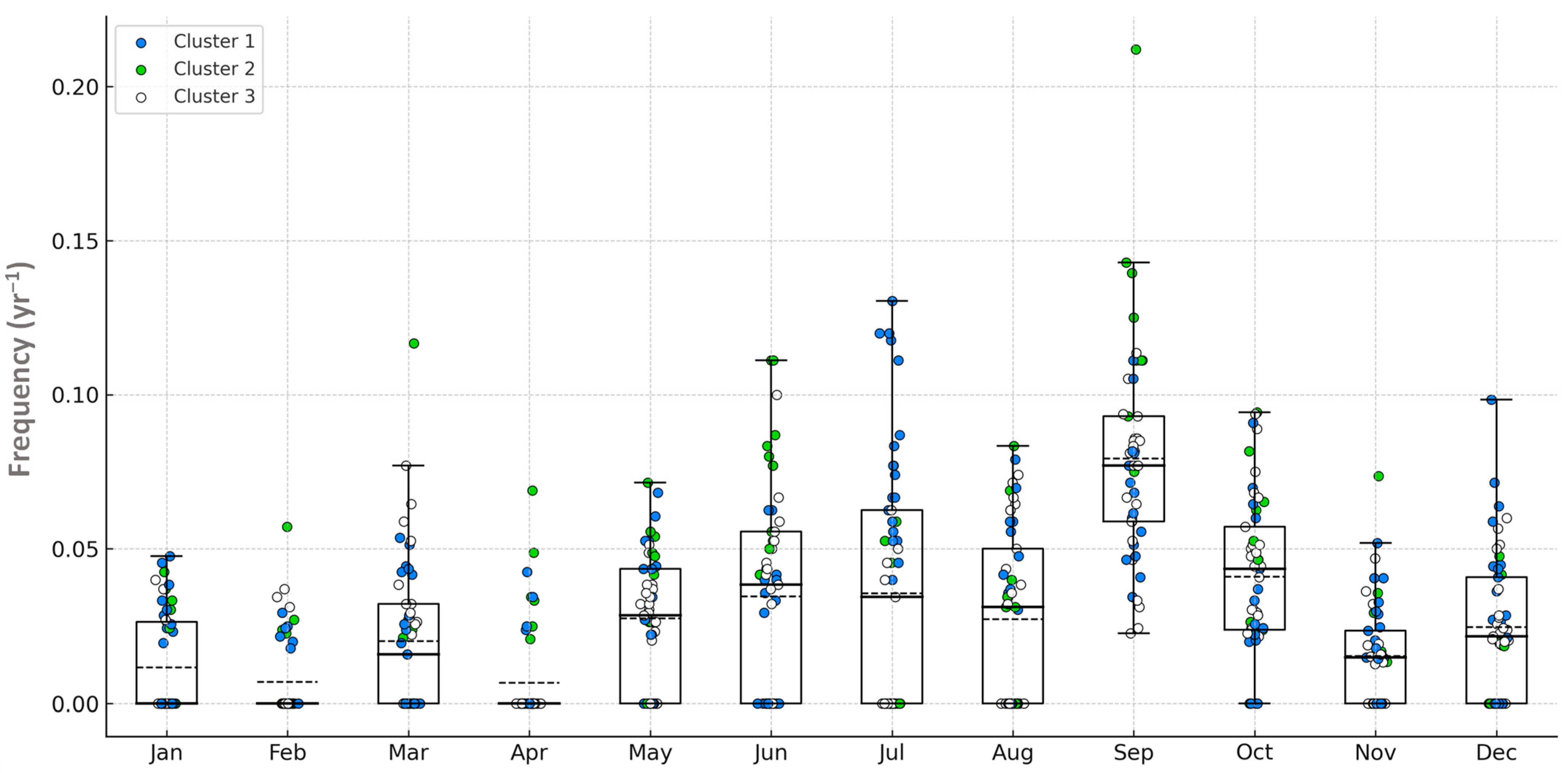
The monthly occurrence frequency of EEs across the 12 months for the 53 stations, ${\lambda }_{EE}\left(k,t\right)$, is shown in Figure A1 using boxplots for each month with overlaid scatter points representing individual station values. ${\lambda }_{EE}\left(k,t\right)$ranges from 0.45 to 3.71 events per year. The month with the highest average frequency (${\overline{\lambda }}_{EE}$) is November (${\overline{\lambda }}_{EE}$ = 2.76 yr⁻¹), while July shows the lowest value (${\overline{\lambda }}_{EE}$= 0.79 yr⁻¹). Among stations, the highest average value is observed at station no. 24 (Monte Cucco), with ${\overline{\lambda }}_{EE}$ = 2.36 month⁻¹, whereas the lowest is at station no. 35 (Petrignano del Lago), with ${\overline{\lambda }}_{EE}$ = 1.14 month⁻¹.

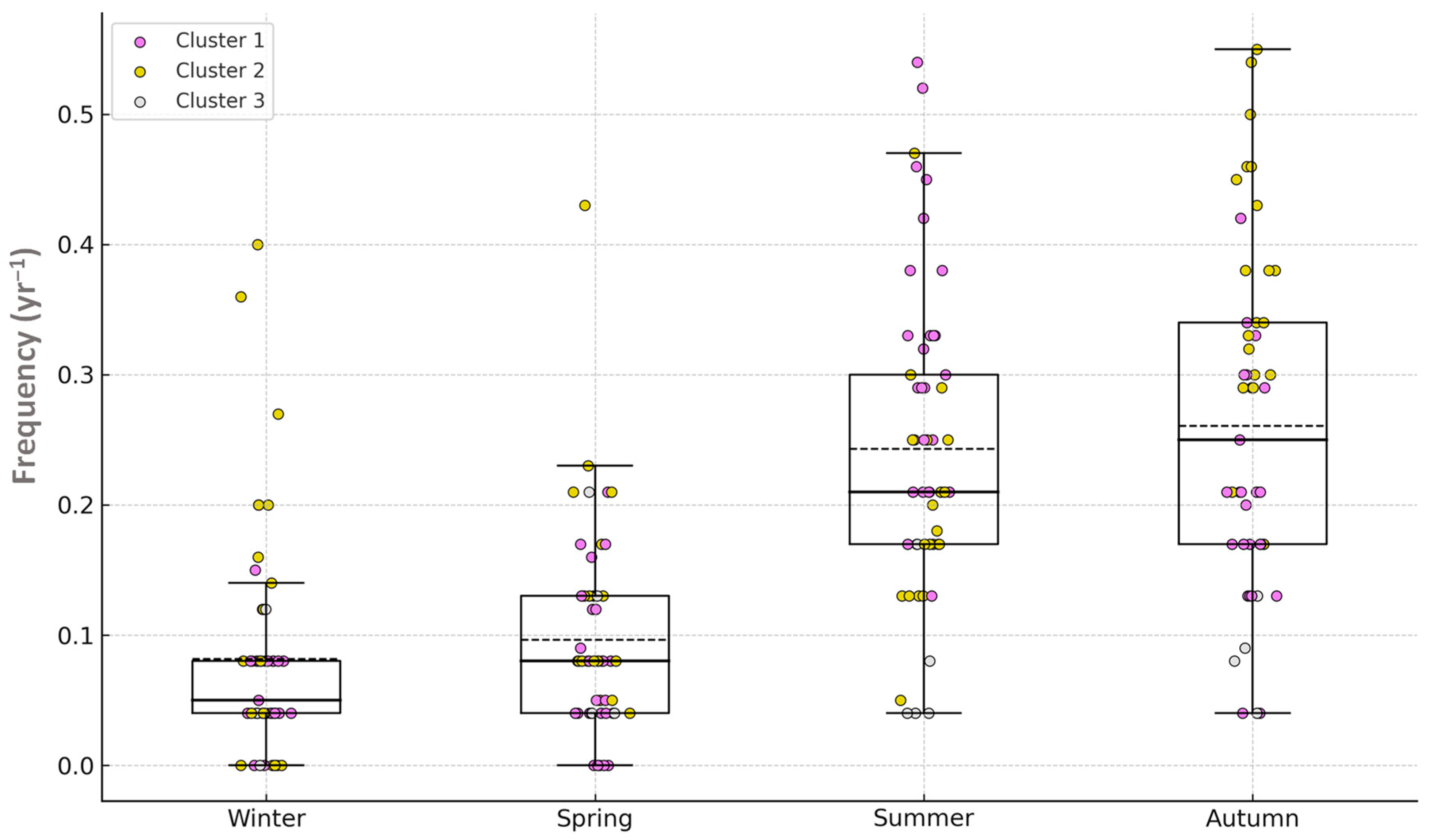
The seasonal occurrence frequency of REs across the 4 seasons for the 53 stations, ${\lambda }_{RE}\left(k,s\right)$, is shown in Figure A2 using boxplots for each season with overlaid scatter points representing individual station values. This frequency ranges from 0 to 0.65 events per year (Figure A2). The season with the highest average frequency ${\overline{\lambda }}_{RE}$ is Autumn (${\overline{\lambda }}_{RE}$ = 0.27 yr⁻¹), followed by Summer with a slightly lower frequency (${\overline{\lambda }}_{RE}$ = 0.24 yr⁻¹), while Winter and Spring show lower frequencies (${\overline{\lambda }}_{RE}$ = 0.08 and 0.10 yr⁻¹, respectively). Among stations, the highest average value is observed at station no. 24 (Monte Cucco), with ${\overline{\lambda }}_{RE}$ = 0.45 season⁻¹, whereas the lowest is at station no. 35 (Petrignano del Lago), with ${\overline{\lambda }}_{RE}$ = 0.04 season⁻¹.

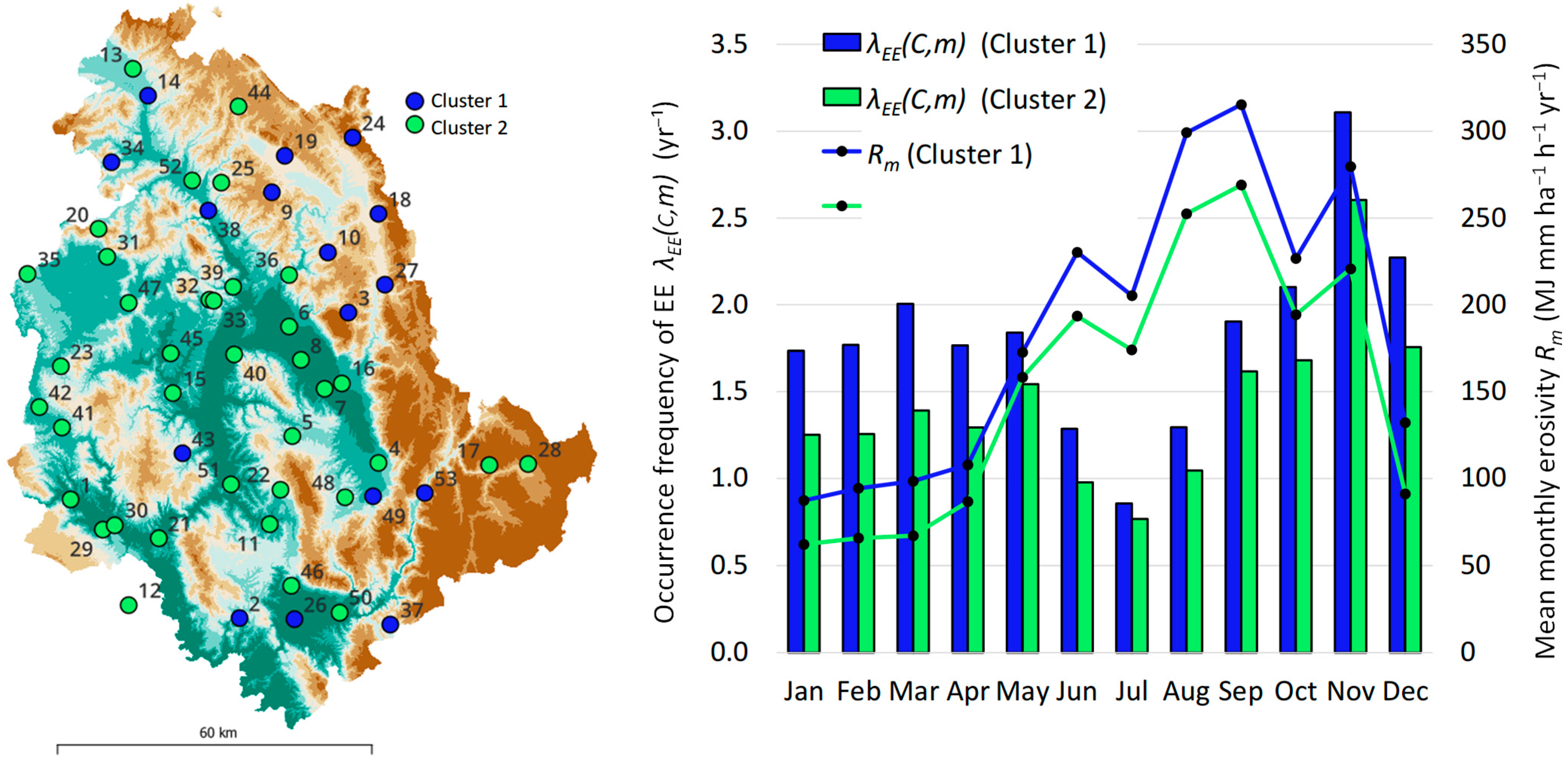
The cluster analysis based on the occurrence of EE identified two groups. The spatial distribution of the two groups and the mean monthly occurrence frequencies of EE, calculated using Equation (3), are shown in Figure 2. Group 1 includes locations with frequencies generally higher than those observed in Group 2. However, the monthly dynamics do not differ significantly, as the Pearson correlation coefficient between the two series of mean monthly values is high, approximately 0.97. The stations belonging to Group 1 are fewer in number than those in Group 2, and they are mainly distributed in the eastern part of the region, along the Apennine ridge, and in the southern area. The only exceptions to this pattern are stations 43, 17, and 28. In Figure 2, for comparison purposes, the mean monthly erosivity ($R_m$), computed according to the USLE procedure [15], for each cluster and month is also shown.

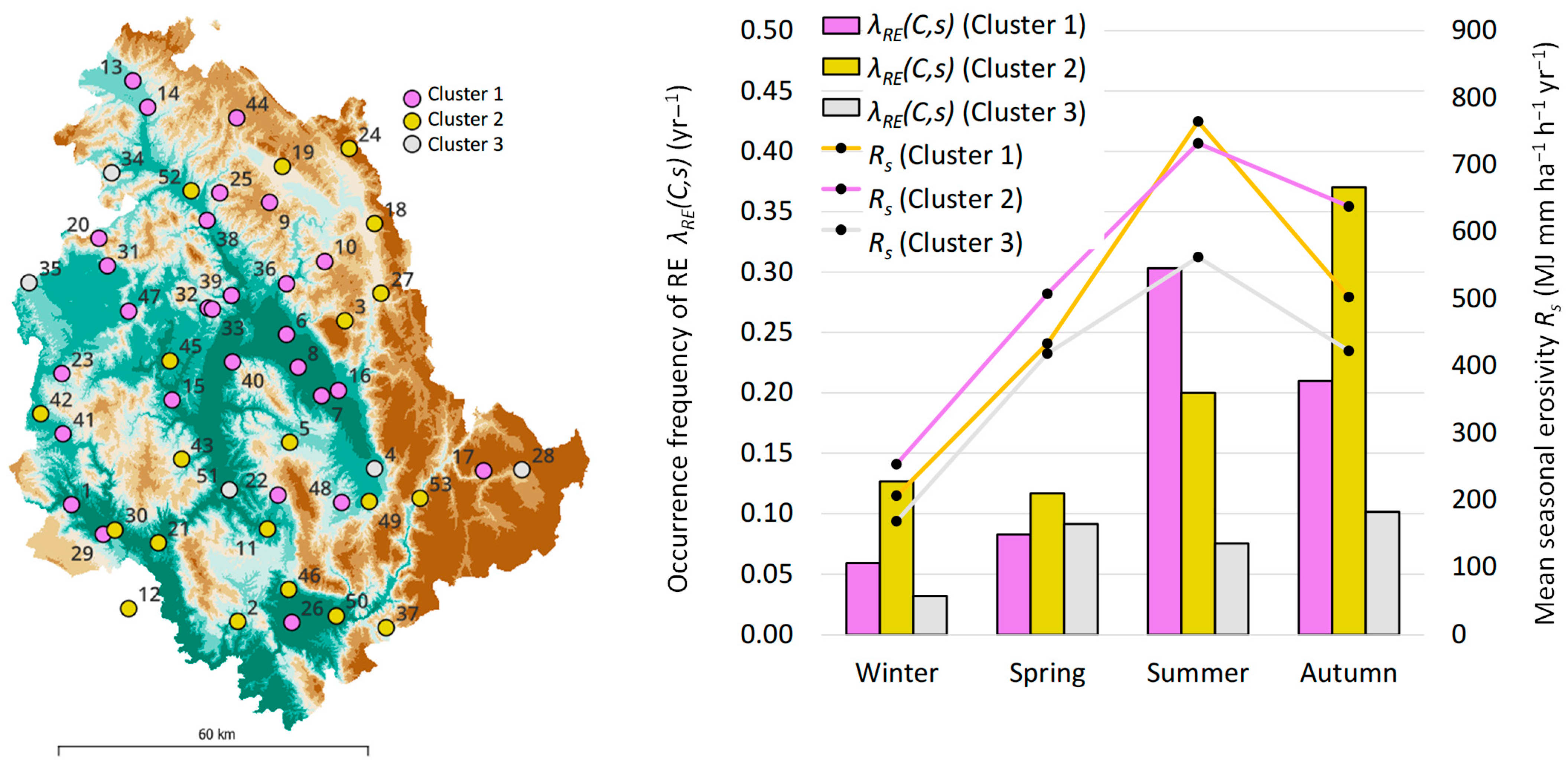
The cluster analysis based on the RE occurrence frequency identified 3 groups (Figure 3). The two most numerous groups are Group 1 and Group 2. Overall, Group 1 exhibits a lower mean frequency of RE compared to Group 2. However, the main difference is observed in the seasonal distribution: Group 1 shows a frequency peak during the summer season, while Group 2 peaks in autumn. Group 3, finally, has much lower frequencies compared to the other two groups, with almost no seasonal differences. From a spatial perspective, no clear pattern is detected. Figure 3 shows, for comparison, the mean seasonal erosivity $R_s$ [15], for each cluster and season.

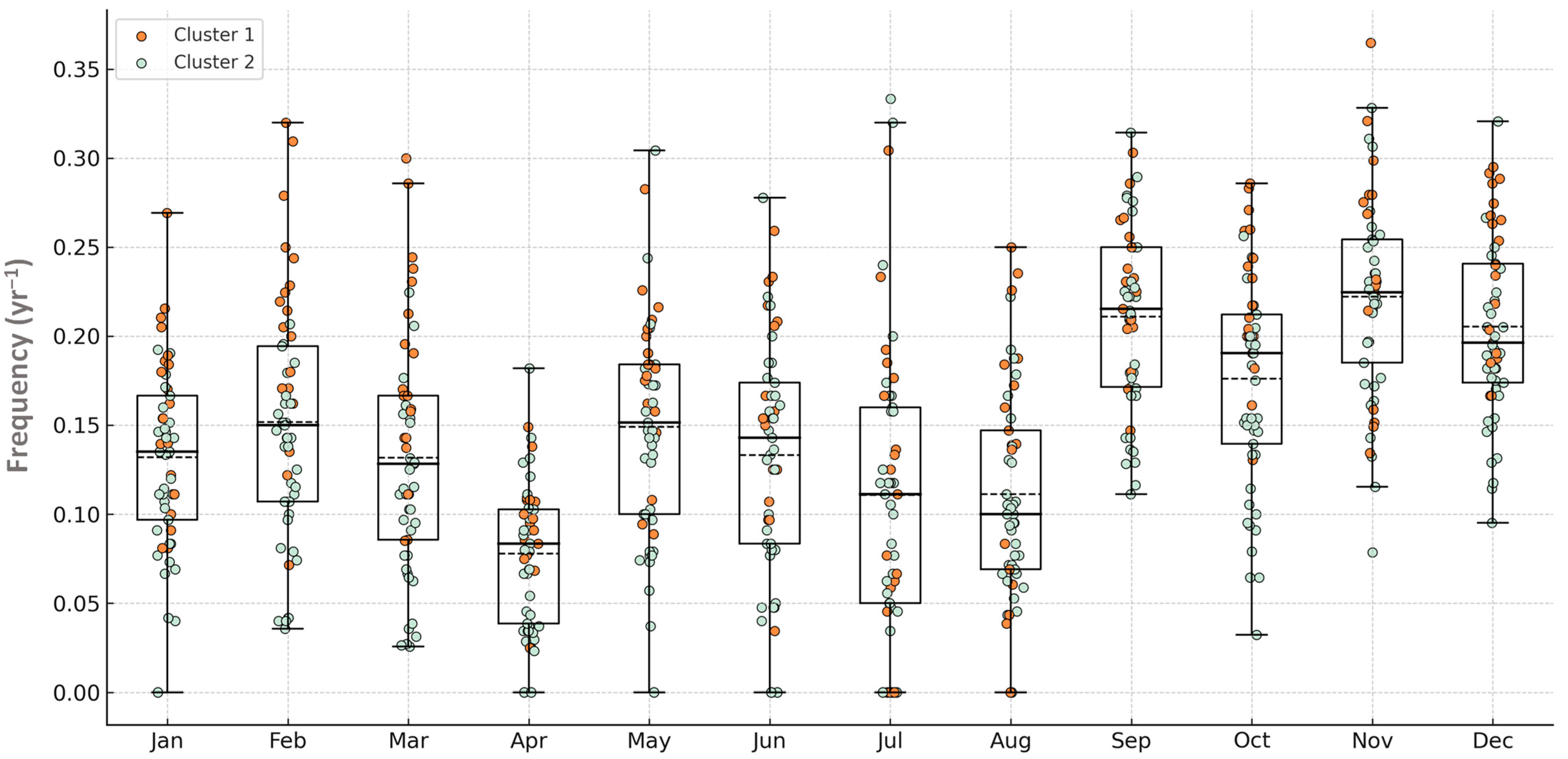
The results concerning the occurrence frequency of consecutive EEs over short time horizons are shown in Figure A3, Figure A4 and Figure A5, respectively, for ${\lambda }_{EE1}\left(k,t\right),$ ${\lambda }_{EE3}\left(k,t\right)$ and ${\lambda }_{EE7}\left(k,t\right)$, using monthly boxplots with overlaid scatter points representing individual station values. It can be observed that the month with the highest average value of ${\lambda }_{EE1}\left(k,t\right),$ (${\overline{\lambda }}_{EE1}$) is September (${\overline{\lambda }}_{EE1}$ = 0.08 yr⁻¹), while the minimum values are observed in February and April, for which ${\overline{\lambda }}_{EE1}$ is about 0.007 yr⁻¹ (Figure A3). As for the stations, the highest average frequency is observed at station no. 3 (Armenzano, ${\overline{\lambda }}_{EE1}$ = 0.053 month⁻¹), while the minimum is observed at station no. 34 (Petrelle) with ${\overline{\lambda }}_{EE1}$ = 0.014 month⁻¹.

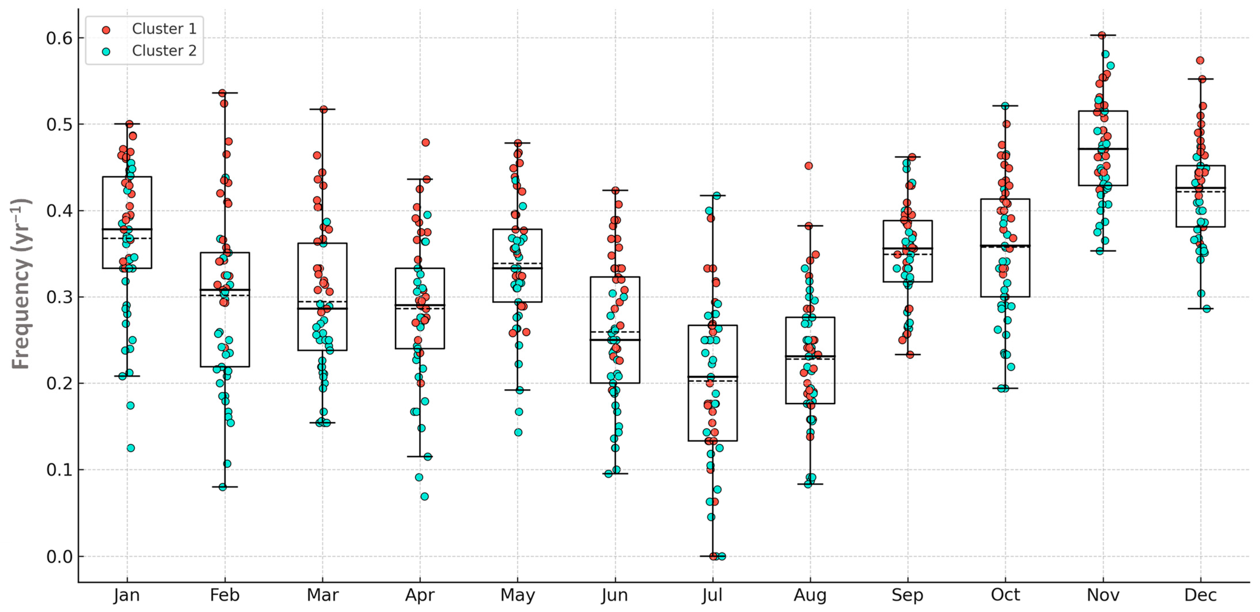
Moving on to consecutive EE events within three days (Figure A4), the month with the highest average value is November (${\overline{\lambda }}_{EE3}$ = 0.22 yr⁻¹), although similarly high values are also observed for September and December, with ${\overline{\lambda }}_{EE3}$ = 0.21 yr⁻¹. Consistent with the previous results, April stands out as a month characterized by a low likelihood of closely spaced consecutive events (${\overline{\lambda }}_{EE3}$ = 0.08 yr⁻¹). As for the stations, the highest average frequency is observed at station no. 9 (Carestello, ${\overline{\lambda }}_{EE3}$ = 0.215 month⁻¹), while the minimum is observed at station no. 40 (Ponte Nuovo) with ${\overline{\lambda }}_{EE3}$ = 0.104 month⁻¹.

Finally, the analysis of ${\lambda }_{EE7}\left(k,t\right)$(Figure A5) shows that November has the highest average value of ${\overline{\lambda }}_{EE7}$ = 0.47 yr⁻¹, while July has the lowest value of ${\overline{\lambda }}_{EE7}$ = 0.20 yr⁻¹.

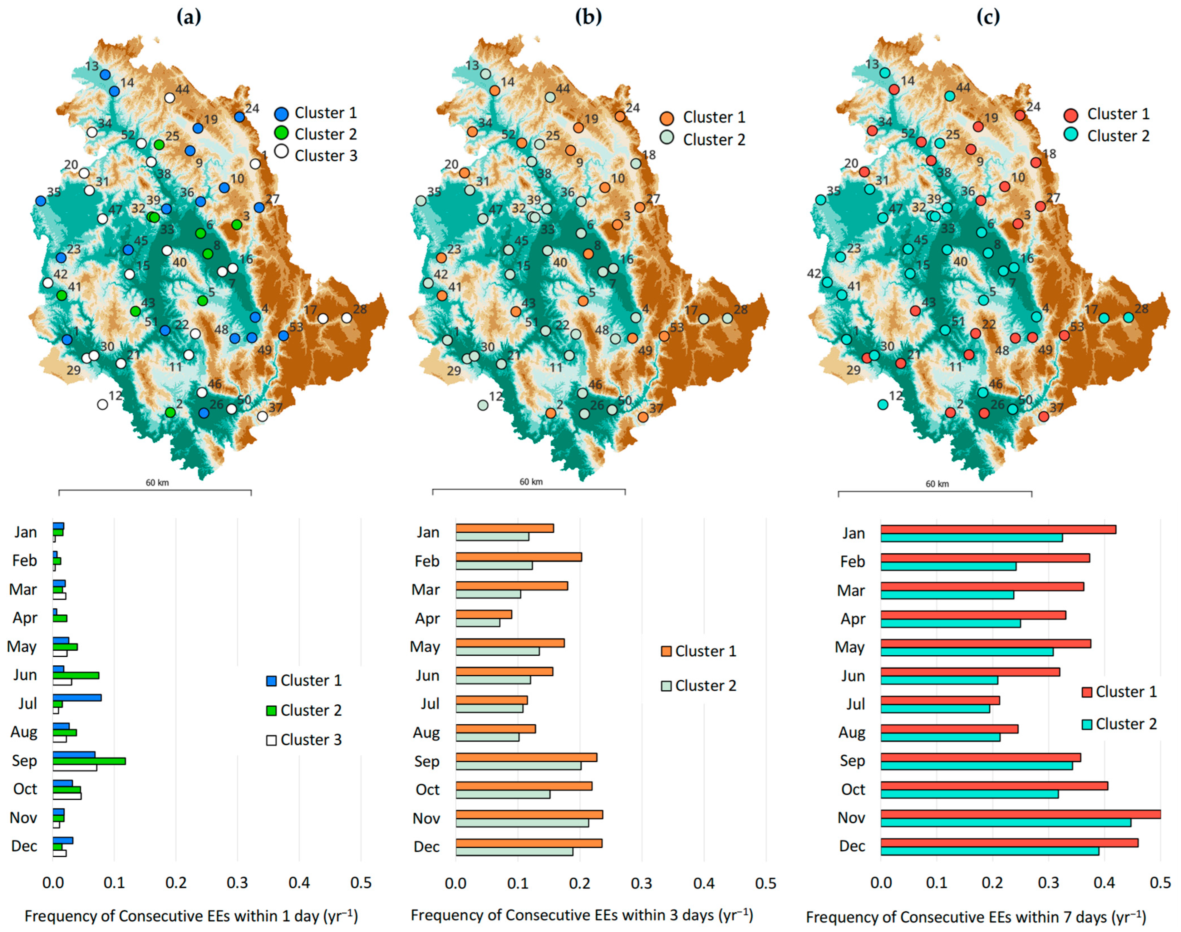
The results of the cluster analysis for ${\lambda }_{EE1}\left(k,t\right),$ ${\lambda }_{EE3}\left(k,t\right)$ and ${\lambda }_{EE7}\left(k,t\right)$ are presented in Figure 4. For ${\lambda }_{EE1}\left(k,t\right)$, three clusters were identified, showing a rather random spatial distribution. The clusters differ both in terms of the overall mean values and in the distribution across the months. Notably, September stands out with relatively high values in all clusters. High frequencies are also observed in June (for Cluster 2) and in July (for Cluster 1). For ${\lambda }_{EE3}\left(k,t\right)$ and ${\lambda }_{EE7}\left(k,t\right)$, two clusters were identified, showing quite similar spatial and temporal distributions. In both cases, Cluster 1 shows lower values than Cluster 2 in almost all months, with minima in July and August (and in April for ${\lambda }_{EE3}\left(k,t\right)$ and maxima in November.

The analysis of trends in the frequency of occurrence of EE and RE events aggregated at the cluster scale did not reveal any significant trend (p-value < 0.05) in any cluster, month, or season, denoting a stationary behavior of the variables in the time series considered.

4. Discussion

Before entering into a detailed discussion of the results, it is important to clarify that this study is based on the adoption of specific threshold values for two rainfall characteristics (P_T = 14.4 mm and P_{max_burst} = 47.4 mm), assumed to discriminate between non-erosive and erosive events and between sheet and rill erosive events, respectively.

Such an assumption can be considered reasonably valid for the experimental site where the thresholds were established (a bare silt loam soil, with a slope of 16%, and plot lengths ranging from 11 to 22 m). Even under these conditions, as highlighted by Todisco et al. (2019) [32], there remains a significant degree of uncertainty, particularly concerning the threshold used to identify the occurrence of rill events.

It should also be emphasized that these threshold values are site-specific and cannot be generalized to other locations without caution. Their application at the regional scale, as carried out in this study, should therefore be interpreted as having a purely climatic significance: the analysis aims to explore how often the climatic conditions leading to such thresholds might occur across different sites and months, assuming the experimental conditions as a standard reference scenario. In this sense, the approach is analogous to that of Wischmeier and Smith [15], who defined a reference experimental plot to characterize rainfall erosivity and soil erodibility independently of local topographic and land-cover factors. The actual frequency of occurrence of EE or RE processes may therefore be higher or lower than that presented here, depending on the specific conditions of the plots. However, the objective of the comparative analysis of such frequencies in space and time (under the same reference conditions) is considered to have been achieved.

The spatial distribution of clusters identified based on λ_EE at each station (Figure 2) reveals a potential dependence on orographic and geographic factors. This relationship was confirmed by a multivariate analysis of variance, which demonstrated a statistically significant effect (p-value < 0.05) of both longitude and altitude on the “cluster group” factor. Specifically, stations in cluster 1 had a mean altitude of 465 m a.s.l. and a mean longitude of 12.57, while those in cluster 2 had a mean altitude of 326 m a.s.l. and a mean longitude of 12.39. In contrast, applying the same type of analysis to λ_RE (Figure 3) and λ_EE1 (Figure 4a) did not reveal any significant contribution from these factors in the identified clusters. For the λ_EE3 clusters (Figure 4b), a significant role of altitude was found, with higher mean values in cluster 1 stations. For the λ_EE7 clusters (Figure 4c), both altitude and longitude affected the cluster, with higher mean values in cluster 1 compared to cluster 2.

The spatial patterns of the clusters associated with λ_EE, λ_EE1, and λ_EE7 appear quite similar to those observed in the same region for mean annual values of rainfall [53] and erosivity [9]. The higher values in the mountainous areas (which in this region lie mostly to the east) (Figure 1) can be attributed to the orographic precipitation enhancement process [54]. In this context, the low values recorded at stations 17 and 28 (Figure 2 and Figure 4) are also consistent, as their inland position may expose them to a classic “rain shadow” effect with respect to frontal systems, which in central Italy predominantly originate from the west (Atlantic) [55]. Conversely, the spatial patterns associated with more extreme rainfall variables (e.g., λ_RE, λ_EE1) exhibit a largely random distribution (Figure 3 and Figure 4a), which may be attributed to the localized and transient nature of convective storms, less dependent on large-scale orographic controls [56]. In addition, the low frequency of occurrence of such extreme events further increases the uncertainty in identifying robust spatial patterns.

The frequency of occurrence of EEs (Figure 2) revealed a monthly temporal pattern only partially corresponding to that of the monthly erosivity factor $R_m$. Specifically, the two dynamics show marked differences between May and September, with relatively low values of ${\lambda }_{EE}$ and high of $R_m$. This outcome is due to the fact that, within the study area, rainfall erosivity is driven by distinct mechanisms in different seasons, being more dependent on the intensity of sporadic events in the summer months and more influenced by rainfall depth and the number of events in other seasons [57]. Consequently, a spatiotemporal characterization of erosive event occurrence based solely on the mean R-factor may be misleading, especially during the spring–summer period. A more comprehensive understanding can be achieved through joint analysis of both the erosivity factor and the frequency with which erosive events can occur in rapid succession. In this study, this aspect was investigated by considering inter-event intervals of 1, 3, and 7 days (Figure 4). Analysis of Figure 4 and Figure 2 shows that the 3- and 7-day intervals (Figure 4b,c) are not particularly informative, as they tend to produce similar spatial and temporal patterns to those obtained with ${\lambda }_{EE}$. In contrast, the 1-day interval ${\lambda }_{EE1}$ (Figure 4a) provides complementary information. For example, months such as June (in Cluster 1) and July (in Cluster 2), which are characterized by low frequencies of erosive events (Figure 2), display relatively high frequencies of ${\lambda }_{EE1}$, indicating a greater likelihood of events occurring in quick succession. The situation in September is especially critical, since it combines medium–high frequencies of erosive events (Figure 2) with high frequencies of closely spaced occurrences. Indeed, several studies using rainfall simulators on plots after initial tillage indicate that, for most soil types and given equivalent rainfall characteristics (depth and intensity), runoff and soil loss tend to increase during subsequent events. This trend is attributed to reduced surface roughness [58], decreased infiltration capacity [59], and the presence of fine material detached in previous events, making it more easily removed.

Regarding the frequency of rill-inducing rainfall events (${\lambda }_{RE}$; Figure 3), two main clusters were identified across the region. Both exhibit relatively lower ${\lambda }_{RE}$ values in winter and spring and higher values during the other seasons; however, the seasonal peak occurs in summer for Cluster 1 and in autumn for Cluster 2. The comparison with the corresponding dynamics of rainfall erosivity ($R_s$) reveals a clear mismatch in spring, during which moderately high $R_s$ values are observed across all clusters. This discrepancy is likely due to the fact that, in this season, erosivity is more strongly influenced by the relatively high frequency of EEs (Figure 2) rather than by the occurrence of extreme rainfall events.

A better agreement between $R_s$ and ${\lambda }_{RE}$ is found in summer and autumn, although for Cluster 2, the timing of the peaks is inverted, with $R_s$ peaking in summer and ${\lambda }_{RE}$ in autumn. This result does not imply that the information derived from the intra-annual distribution of the mean R-factor is incorrect. Rather, it highlights that a spatiotemporal characterization of the frequency of events exceeding specific erosion-triggering thresholds can provide more detailed and complementary insights compared to those offered by the mean R-factor. The key distinction lies in the fact that the former represents a more event-based approach, as opposed to one relying solely on average erosivity values. This is particularly relevant given the recognized impact that isolated extreme events can have on total annual soil loss [18]. Specifically, rill events, due to the action of concentrated flow, tend to mobilize much larger sediment volumes than inter-rill events, thereby causing greater loss of fertile soil and more severe degradation of soil structure. This is particularly detrimental in agricultural landscapes, leading to reduced soil productivity, higher fertilizer and land management costs, and an increased risk of water contamination from eroded sediments and associated agrochemicals [60]. Several studies (e.g., [61,62]) indicate that rill erosion can account for about 70% of total soil loss, despite being less frequent than inter-rill erosion. For example, in the study by Pampalone et al. [26], within a database of more than 700 monitored events (of which only 16% involved rill processes), rill events contributed 64% of the total soil loss. In our case, the proportion of events classified as rill relative to the total number of erosive events (rill + inter-rill) is only 4% (Table 1). This difference, when compared with studies such as Pampalone et al. [26], is mainly related not to the actual number of rill events but to the total number of erosive events detected. In our modeling framework, the identification threshold is applied synthetically to each individual rainfall event, which results in a larger number of total erosive events. By contrast, in experimental conditions, as noted by Todisco et al. [32], a monitored erosive event often includes several consecutive individual rainfall events grouped together, thereby reducing the overall number of recorded erosive events.

No significant temporal trends emerged from the analysis of annual series (2000–2024) for the two main variables considered (${\lambda }_{EE}$ and ${\lambda }_{RE}$). Although no studies specifically addressing these variables are found in the literature, comparisons can be drawn with trend analyses focused on related variables, such as rainfall erosivity or rainfall intensity. Regarding rainfall erosivity, the absence of trends in the investigated variables aligns—as expected—with previous work conducted on the same dataset [9], where analysis of annual values of the USLE erosivity factor revealed generally stationary conditions. Other studies based on longer historical series, however, have highlighted the presence of positive erosivity trends within the study area [63]. Investigations in other Italian regions using rainfall intensity indicators have shown highly variable situations, both spatially and seasonally [20,64,65]. Nevertheless, any discrepancies between the trend analysis performed in this study and findings from the literature are thought to be mainly attributable to the relatively short historical series, which is limited in characterizing long-term trends. On the other hand, as recently highlighted by Vicente-Serrano et al. [66], the rainfall regime in Mediterranean areas appears to be characterized more by temporal variability (i.e., alternating wet and dry periods) than by the presence of actual trends.

Limitations and Future Perspectives

The rainfall thresholds were identified from a large experimental dataset collected under specific reference conditions. Consequently, the occurrence frequencies derived from these data have a certain degree of reliability only for soil, slope and land-use conditions similar to those under which they were originally obtained. Even with this premise, some uncertainty remains. As shown by Todisco et al. (2019) [32], even the best-performing variables and thresholds do not allow for event-type classifications that are completely error-free.

Furthermore, the observational database used to derive the thresholds is numerically limited with respect to rill events. Future applications should therefore include an expansion of the observational dataset under the same reference conditions, together with an experimental validation (using new data) of the effectiveness of the proposed thresholds in classifying events.

An even more valuable—although considerably more demanding in terms of effort and resources—future development would be the implementation of monitoring campaigns across different combinations of soil types and slope gradients. In particular, the soil type of the experimental site from which the rainfall thresholds were derived (silty–clay–loam) represents only 12% of those occurring in the Umbria region, where textures such as clay–loam (69%) and loam (17%) are far more common [40].

Such an extended monitoring framework would not only improve the robustness and transferability of the thresholds but also provide insight into their sensitivity to varying physical and hydrological conditions. This, in turn, could support the development of more generalizable or site-specific predictive tools for event classification.

5. Conclusions

This study examined 24 years of high-resolution rainfall data from 53 stations across Umbria to quantify how often rainfall conditions capable of triggering erosive processes actually occur at the regional scale. The analysis focused on a set of rainfall characteristics—previously validated as effective indicators of general erosive events (EE) and rill erosion events (RE) under controlled soil–slope–land-use conditions—and used them as operational thresholds for event identification.

The mean frequency of EEs varies by a factor of two among stations, ranging from roughly 1 to more than 2 events per month, whereas rill-related events are far less common, with seasonal averages spanning from about 0.04 to 0.45 events. Spatial clustering analyses further clarify these patterns. EE frequencies tend to be higher in the mountainous sectors of Umbria, mirroring the well-known distribution of annual precipitation and reflecting a clear orographic influence. By contrast, the spatial distribution of REs does not exhibit equally interpretable patterns, suggesting that more extreme erosive responses may depend on localized factors not captured by regional-scale rainfall gradients.

Seasonal analyses highlight critical windows for soil protection. EE frequencies peak in autumn (around 6.5 events yr⁻¹) and remain high in winter (about 4.5 events yr⁻¹). September, in particular, shows the highest probability of closely spaced EE occurrences (within 24 h), with a mean frequency of about 0.1 yr⁻¹. When focusing on the more extreme and impactful events (REs), the seasonal pattern differs markedly from that of EEs: RE frequencies reach their minimum in winter (~0.08 yr⁻¹) and increase during summer and early autumn, reaching up to ~0.26 yr⁻¹ when soil cover is typically sparse. These findings emphasize the importance of aligning conservation practices with the specific seasonal susceptibility of different erosion processes.

No significant long-term changes emerge over the observation period, suggesting stable climatic forcing with respect to the rainfall attributes that control erosive dynamics. Comparisons with the temporal behavior of the USLE R-factor further show that rainfall erosivity alone does not adequately reproduce the monthly and seasonal patterns of either EE or RE frequencies, indicating that threshold-based indicators capture aspects of event generation not reflected in traditional erosivity metrics.

Practical Implications

The most relevant practical outcome of this study concerns the identification of periods in the year with a high risk of EE and RE occurrence. For instance, September and the autumn months appear particularly critical, with frequent RE events and EE events that may occur frequently and even consecutively. From an agronomic perspective, these periods are especially vulnerable. In fields intended for winter cereals, this is the time when land preparation for sowing typically occurs, leaving soils bare or poorly covered and therefore highly exposed to erosion.

In systems where summer crops are the main cultivation, soils are often left fallow or sown with cover crops as part of farmers’ adherence to agro-environmental measures. However, even in these cases, soil preparation for cover crop seeding involves tillage that can increase the soil’s susceptibility to erosion compared to conventional management, which typically entails only coarse surface preparation. Such critical aspects related to cover crop use have already been noted by [34] and are confirmed here, given the concomitant high risk of erosive events.

A practical solution might therefore consist of combining cover crop adoption with minimum tillage practices and selecting fast-growing species to minimize the probability of severe erosive events during periods when the soil lacks adequate protection. The usefulness of the event-based approach is further reinforced, as it provides a more realistic insight than analyses based on long-term averages, which may identify conditions as being similar despite producing very different impacts. In particular, a single RE occurring in the weeks following cover crop sowing could be harmful not only because of the associated soil loss but also due to its likely adverse effects on crop establishment and early development.

References

1. Cerdan, O.; Govers, G.; Le Bissonnais, Y.; Van Oost, K.; Poesen, J.; Saby, N.; Gobin, A.; Vacca, A.; Quinton, J.; Auerswald, K.; et al. Rates and Spatial Variations of Soil Erosion in Europe: A Study Based on Erosion Plot Data. Geomorphology 2010, 122, 167–177. [Google Scholar] [CrossRef]
2. Ferreira, C.S.S.; Seifollahi-Aghmiuni, S.; Destouni, G.; Ghajarnia, N.; Kalantari, Z. Soil Degradation in the European Mediterranean Region: Processes, Status and Consequences. Sci. Total Environ. 2022, 805, 150106. [Google Scholar] [CrossRef] [PubMed]
3. Piacentini, T.; Galli, A.; Marsala, V.; Miccadei, E. Analysis of Soil Erosion Induced by Heavy Rainfall: A Case Study from the NE Abruzzo Hills Area in Central Italy. Water 2018, 10, 1314. [Google Scholar] [CrossRef]
4. Bufalini, M.; Materazzi, M.; Martinello, C.; Rotigliano, E.; Pambianchi, G.; Tromboni, M.; Paniccià, M. Soil Erosion and Deposition Rate Inside an Artificial Reservoir in Central Italy: Bathymetry versus RUSLE and Morphometry. Land 2022, 11, 1924. [Google Scholar] [CrossRef]
5. Costantini, E.A.C.; Lorenzetti, R. Soil Degradation Processes in the Italian Agricultural and Forest Ecosystems. Ital. J. Agron. 2013, 8, e28. [Google Scholar] [CrossRef]
6. Panagos, P.; Ballabio, C.; Himics, M.; Scarpa, S.; Matthews, F.; Bogonos, M.; Poesen, J.; Borrelli, P. Projections of Soil Loss by Water Erosion in Europe by 2050. Environ. Sci. Policy 2021, 124, 380–392. [Google Scholar] [CrossRef]
7. Panagos, P.; Ballabio, C.; Borrelli, P.; Meusburger, K. Spatio-Temporal Analysis of Rainfall Erosivity and Erosivity Density in Greece. CATENA 2016, 137, 161–172. [Google Scholar] [CrossRef]
8. Vásquez, C.; Klik, A.; Stumpp, C.; Laaha, G.; Strauss, P.; Özcelik, N.B.; Pistotnik, G.; Yin, S.; Dostal, T.; Gaona, G.; et al. Rainfall Erosivity across Austria’s Main Agricultural Areas: Identification of Rainfall Characteristics and Spatiotemporal Patterns. J. Hydrol. Reg. Stud. 2024, 53, 101770. [Google Scholar] [CrossRef]
9. Todisco, F.; Massimi Alunno, A.; Vergni, L. Spatial Distribution, Temporal Behaviour, and Trends of Rainfall Erosivity in Central Italy Using Coarse Data. Water 2025, 17, 801. [Google Scholar] [CrossRef]
10. Angulo-Martínez, M.; Beguería, S. Trends in Rainfall Erosivity in NE Spain at Annual, Seasonal and Daily Scales, 1955–2006. Hydrol. Earth Syst. Sci. 2012, 16, 3551–3559. [Google Scholar] [CrossRef]
11. Uber, M.; Haller, M.; Brendel, C.; Hillebrand, G.; Hoffmann, T. Past, Present and Future Rainfall Erosivity in Central Europe Based on Convection-Permitting Climate Simulations. Hydrol. Earth Syst. Sci. 2024, 28, 87–102. [Google Scholar] [CrossRef]
12. Woldegebrael, S.M.; Romano, N.; Pumo, D.; Deidda, R.; Ippolito, M.; Cannarozzo, M.; Langousis, A.; Serafeim, A.V.; Manfreda, S.; Nasta, P. Empirical Approaches to Estimate Rainfall Erosivity from Coarse Temporal Resolution Precipitation Data in the Mediterranean Region. Sci. Total Environ. 2025, 996, 180122. [Google Scholar] [CrossRef]
13. Dallan, E.; Bagarello, V.; Ferro, V.; Pampalone, V.; Borga, M. Evaluation and Projected Changes in Rainfall Erosivity: Topography Dependence Revealed by Convection-Permitting Climate Projections for the Mediterranean Island of Sicily. CATENA 2025, 254, 108975. [Google Scholar] [CrossRef]
14. Padulano, R.; Santini, M.; Mancini, M.; Stojiljkovic, M.; Rianna, G. Monthly to Seasonal Rainfall Erosivity over Italy: Current Assessment by Empirical Model and Future Projections by EURO-CORDEX Ensemble. CATENA 2023, 223, 106943. [Google Scholar] [CrossRef]
15. Wischmeier, W.H.; Smith, D.D. Predicting Rainfall-Erosion Losses: A Guide to Conservation Farming; U.S. Department of Agriculture, Science and Education Administration: Washington, DC, USA, 1978.
16. Di Lena, B.; Curci, G.; Vergni, L. Analysis of Rainfall Erosivity Trends 1980–2018 in a Complex Terrain Region (Abruzzo, Central Italy) from Rain Gauges and Gridded Datasets. Atmosphere 2021, 12, 657. [Google Scholar] [CrossRef]
17. Padulano, R.; Rianna, G.; Santini, M. Datasets and Approaches for the Estimation of Rainfall Erosivity over Italy: A Comprehensive Comparison Study and a New Method. J. Hydrol. Reg. Stud. 2021, 34, 100788. [Google Scholar] [CrossRef]
18. Wei, L.; Peng, X.; Fu, Y.; Gu, Z.; Liang, G.; Miao, C.; Dai, Q. Reveal of Contributing Rainfalls to Annual Soil Erosion and the Response of Runoff Sediment Output: A Case of Zonal Yellow Soil Area. J. Hydrol. 2025, 652, 132666. [Google Scholar] [CrossRef]
19. Diodato, N.; Gómara, I.; Baronetti, A.; Fratianni, S.; Bellocchi, G. Reconstruction of Erosivity Density in Northwest Italy since 1701. Hydrol. Sci. J. 2021, 66, 1185–1196. [Google Scholar] [CrossRef]
20. Avino, A.; Cimorelli, L.; Furcolo, P.; Noto, L.V.; Pelosi, A.; Pianese, D.; Villani, P.; Manfreda, S. Are Rainfall Extremes Increasing in Southern Italy? J. Hydrol. 2024, 631, 130684. [Google Scholar] [CrossRef]
21. De Luca, D.L.; Ridolfi, E.; Russo, F.; Moccia, B.; Napolitano, F. Climate Change Effects on Rainfall Extreme Value Distribution: The Role of Skewness. J. Hydrol. 2024, 634, 130958. [Google Scholar] [CrossRef]
22. Wirtz, S.; Seeger, M.; Ries, J.B. Field Experiments for Understanding and Quantification of Rill Erosion Processes. CATENA 2012, 91, 21–34. [Google Scholar] [CrossRef]
23. Zhang, X.J. Roles of Raindrop Impact in Detachment and Transport Processes of Interrill Soil Erosion. Int. Soil Water Conserv. Res. 2023, 11, 592–601. [Google Scholar] [CrossRef]
24. Morgan, R.P.C.; Quinton, J.N.; Smith, R.E.; Govers, G.; Poesen, J.W.A.; Auerswald, K.; Chisci, G.; Torri, D.; Styczen, M.E. The European Soil Erosion Model (EUROSEM): A Dynamic Approach for Predicting Sediment Transport from Fields and Small Catchments. Earth Surf. Process. Landf. 1998, 23, 527–544. [Google Scholar] [CrossRef]
25. Flanagan, D.C.; Nearing, M.A. USDA Water Erosion Prediction Project: Hillslope Profile and Watershed Model Documentation; NSERL Report No. 10 1995; USDA-ARS National Soil Erosion Research Laboratory: West Lafayette, IN, USA, 1995.
26. Pampalone, V.; Nicosia, A.; Palmeri, V.; Serio, M.A.; Ferro, V. Rill and Interrill Soil Loss Estimations Using the USLE-MB Equation at the Sparacia Experimental Site (South Italy). Water 2023, 15, 2396. [Google Scholar] [CrossRef]
27. Berger, C.; Schulze, M.; Rieke-Zapp, D.; Schlunegger, F. Rill Development and Soil Erosion: A Laboratory Study of Slope and Rainfall Intensity. Earth Surf. Process. Landf. 2010, 35, 1456–1467. [Google Scholar] [CrossRef]
28. Shen, H.; Zheng, F.; Wen, L.; Han, Y.; Hu, W. Impacts of Rainfall Intensity and Slope Gradient on Rill Erosion Processes at Loessial Hillslope. Soil Tillage Res. 2016, 155, 429–436. [Google Scholar] [CrossRef]
29. Yan, Y.; Tu, N.; Cen, L.; Gan, F.; Dai, Q.; Mei, L. Characteristics and Dynamic Mechanism of Rill Erosion Driven by Extreme Rainfall on Karst Plateau Slopes, SW China. CATENA 2024, 238, 107890. [Google Scholar] [CrossRef]
30. Pan, J.; Li, P.; Xu, Y.; Cao, Y.; Ren, Z.; Zhou, S.; Lu, K. The Response of Slope Hydrodynamics and Rill Development to Erosion in the Water-Wind Erosion Crisscross Region of the Loess Plateau, China. CATENA 2025, 261, 109590. [Google Scholar] [CrossRef]
31. Xie, Y.; Liu, B.; Nearing, M.A. Practical Thresholds for Separating Erosive and Nonerosive Storms. Trans. ASAE 2002, 45, 1843–1847. [Google Scholar] [CrossRef]
32. Todisco, F.; Vergni, L.; Vinci, A.; Pampalone, V. Practical Thresholds to Distinguish Erosive and Rill Rainfall Events. J. Hydrol. 2019, 579, 124173. [Google Scholar] [CrossRef]
33. Abdelwahab, O.M.M.; Ricci, G.F.; Gentile, F.; De Girolamo, A.M. Modelling the Impact of Climate Change on Runoff and Sediment Yield in Mediterranean Basins: The Carapelle Case Study (Apulia, Italy). Front. Water 2025, 7, 1486644. [Google Scholar] [CrossRef]
34. López-Vicente, M.; Gómez, J.A.; Guzmán, G.; Calero, J.; García-Ruiz, R. The Role of Cover Crops in the Loss of Protected and Non-Protected Soil Organic Carbon Fractions Due to Water Erosion in a Mediterranean Olive Grove. Soil Tillage Res. 2021, 213, 105119. [Google Scholar] [CrossRef]
35. Alliaume, F.; Rossing, W.A.H.; Tittonell, P.; Jorge, G.; Dogliotti, S. Reduced Tillage and Cover Crops Improve Water Capture and Reduce Erosion of Fine Textured Soils in Raised Bed Tomato Systems. Agric. Ecosyst. Environ. 2014, 183, 127–137. [Google Scholar] [CrossRef]
36. Chen, L.; Rejesus, R.M.; Aglasan, S.; Hagen, S.C.; Salas, W. The Impact of Cover Crops on Soil Erosion in the US Midwest. J. Environ. Manag. 2022, 324, 116168. [Google Scholar] [CrossRef]
37. Fendrich, A.N.; Matthews, F.; Van Eynde, E.; Carozzi, M.; Li, Z.; d’Andrimont, R.; Lugato, E.; Martin, P.; Ciais, P.; Panagos, P. From Regional to Parcel Scale: A High-Resolution Map of Cover Crops across Europe Combining Satellite Data with Statistical Surveys. Sci. Total Environ. 2023, 873, 162300. [Google Scholar] [CrossRef]
38. Machiwal, D.; Kumar, S.; Islam, A.; Kumar, S.; Jat, S.R.; Vaishnav, M.; Dayal, D. Evaluating Effect of Cover Crops on Runoff, Soil Loss and Soil Nutrients in an Indian Arid Region. Commun. Soil Sci. Plant Anal. 2021, 52, 1669–1688. [Google Scholar] [CrossRef]
39. Kaye, J.P.; Quemada, M. Using Cover Crops to Mitigate and Adapt to Climate Change. A Review. Agron. Sustain. Dev. 2017, 37, 4. [Google Scholar] [CrossRef]
40. Vergni, L.; Pasquini, N.; Todisco, F. Best Siting for Small Hill Reservoirs and the Challenge of Sedimentation: A Case Study in the Umbria Region (Central Italy). Land 2025, 14, 1401. [Google Scholar] [CrossRef]
41. Tarquini, S.; Isola, I.; Favalli, M.; Battistini, A.; Dotta, G. TINITALY, a Digital Elevation Model of Italy with a 10 Meters Cell Size, Version 1.1; Istituto Nazionale di Geofisica e Vulcanologia: Rome, Italy, 2023. [Google Scholar] [CrossRef]
42. Di Stefano, C.; Pampalone, V.; Todisco, F.; Vergni, L.; Ferro, V. Testing the Universal Soil Loss Equation-MB Equation in Plots in Central and South Italy. Hydrol. Process. 2019, 33, 2422–2433. [Google Scholar] [CrossRef]
43. Todisco, F. The Internal Structure of Erosive and Non-Erosive Storm Events for Interpretation of Erosive Processes and Rainfall Simulation. J. Hydrol. 2014, 519, 3651–3663. [Google Scholar] [CrossRef]
44. Panagos, P.; Borrelli, P.; Spinoni, J.; Ballabio, C.; Meusburger, K.; Beguería, S.; Klik, A.; Michaelides, S.; Petan, S.; Hrabalíková, M.; et al. Monthly Rainfall Erosivity: Conversion Factors for Different Time Resolutions and Regional Assessments. Water 2016, 8, 119. [Google Scholar] [CrossRef]
45. Vergni, L.; Vinci, A.; Todisco, F. Influence of the Rainfall Time Step on the Thresholds for Separating Erosive and Non-Erosive Events. In AIIA 2022: Biosystems Engineering Towards the Green Deal; Ferro, V., Giordano, G., Orlando, S., Vallone, M., Cascone, G., Porto, S.M.C., Eds.; Lecture Notes in Civil Engineering; Springer International Publishing: Cham, Switzerland, 2023; Volume 337, pp. 211–219. ISBN 978-3-031-30328-9. [Google Scholar]
46. Piccarreta, M.; Lazzari, M.; Bentivenga, M. The Influence in Rainfall Erosivity Calculation by Using Different Temporal Resolution in Mediterranean Area. Sci. Total Environ. 2024, 906, 167411. [Google Scholar] [CrossRef]
47. Ward, J.H. Hierarchical Grouping to Optimize an Objective Function. J. Am. Stat. Assoc. 1963, 58, 236–244. [Google Scholar] [CrossRef]
48. Rousseeuw, P.J. Silhouettes: A Graphical Aid to the Interpretation and Validation of Cluster Analysis. J. Comput. Appl. Math. 1987, 20, 53–65. [Google Scholar] [CrossRef]
49. Hamed, K.H. Trend Detection in Hydrologic Data: The Mann–Kendall Trend Test under the Scaling Hypothesis. J. Hydrol. 2008, 349, 350–363. [Google Scholar] [CrossRef]
50. Yue, S.; Wang, C. The Mann-Kendall Test Modified by Effective Sample Size to Detect Trend in Serially Correlated Hydrological Series. Water Resour. Manag. 2004, 18, 201–218. [Google Scholar] [CrossRef]
51. Maechler, M.; Rousseeuw, P.; Struyf, A.; Hubert, M. cluster: “Finding Groups in Data”: Cluster Analysis Extended Rousseeuw et al. 1999, Version 2.1.8.1.; R Foundation for Statistical Computing: Vienna, Austria, 2025. [Google Scholar] [CrossRef]
52. Pohlert, T. trend: Non-Parametric Trend Tests and Change-Point Detection 2015, Version 1.1.6; R Foundation for Statistical Computing: Vienna, Austria, 2023. [Google Scholar] [CrossRef]
53. Cardinali, M.; Galli, M.; Guzzetti, F.; Ardizzone, F.; Reichenbach, P.; Bartoccini, P. Rainfall Induced Landslides in December 2004 in South-Western Umbria, Central Italy: Types, Extent, Damage and Risk Assessment. Nat. Hazards Earth Syst. Sci. 2006, 6, 237–260. [Google Scholar] [CrossRef]
54. Roe, G.H. OROGRAPHIC PRECIPITATION. Annu. Rev. Earth Planet. Sci. 2005, 33, 645–671. [Google Scholar] [CrossRef]
55. Nigro, M.; Barsanti, M.; Raco, B.; Giannecchini, R. Investigating a Century of Rainfall: The Impact of Elevation on Precipitation Changes (Northern Tuscany, Italy). Water 2024, 16, 2866. [Google Scholar] [CrossRef]
56. Cipolla, G.; Francipane, A.; Noto, L.V. Classification of Extreme Rainfall for a Mediterranean Region by Means of Atmospheric Circulation Patterns and Reanalysis Data. Water Resour. Manag. 2020, 34, 3219–3235. [Google Scholar] [CrossRef]
57. Vergni, L.; Todisco, F. Bivariate Analysis of Rainfall Characteristics for Identifying Soil Loss Return Periods at the Event Scale. J. Hydrol. 2026, 664, 134605. [Google Scholar] [CrossRef]
58. Vinci, A.; Todisco, F.; Vergni, L.; Torri, D. A Comparative Evaluation of Random Roughness Indices by Rainfall Simulator and Photogrammetry. CATENA 2020, 188, 104468. [Google Scholar] [CrossRef]
59. Todisco, F.; Vergni, L.; Iovino, M.; Bagarello, V. Changes in Soil Hydrodynamic Parameters during Intermittent Rainfall Following Tillage. CATENA 2023, 226, 107066. [Google Scholar] [CrossRef]
60. Zema, D.A. Understanding, Measuring, Mitigating and Modeling Rill Erosion: A Short Review. Earth Environ. Sustain. 2025, 1, 59–70. [Google Scholar] [CrossRef]
61. Govers, G.; Poesen, J. Assessment of the Interrill and Rill Contributions to Total Soil Loss from an Upland Field Plot. Geomorphology 1988, 1, 343–354. [Google Scholar] [CrossRef]
62. Zhang, X.; Liu, G.; Zheng, F. Understanding Erosion Processes Using Rare Earth Element Tracers in a Preformed Interrill-Rill System. Sci. Total Environ. 2018, 625, 920–927. [Google Scholar] [CrossRef]
63. Bezak, N.; Ballabio, C.; Mikoš, M.; Petan, S.; Borrelli, P.; Panagos, P. Reconstruction of Past Rainfall Erosivity and Trend Detection Based on the REDES Database and Reanalysis Rainfall. J. Hydrol. 2020, 590, 125372. [Google Scholar] [CrossRef]
64. Capozzi, V.; Rocco, A.; Annella, C.; Cretella, V.; Fusco, G.; Budillon, G. Signals of Change in the Campania Region Rainfall Regime: An Analysis of Extreme Precipitation Indices (2002–2021). Meteorol. Appl. 2023, 30, e2168. [Google Scholar] [CrossRef]
65. Luppichini, M.; Bini, M. Evolution of Rainfall in Italy over the Last 200 Years: Interactions between Climate Indices and Global Warming. Atmospheric Res. 2025, 326, 108276. [Google Scholar] [CrossRef]
66. Vicente-Serrano, S.M.; Tramblay, Y.; Reig, F.; González-Hidalgo, J.C.; Beguería, S.; Brunetti, M.; Kalin, K.C.; Patalen, L.; Kržič, A.; Lionello, P.; et al. High Temporal Variability Not Trend Dominates Mediterranean Precipitation. Nature 2025, 639, 658–666. [Google Scholar] [CrossRef]
Figure 1. Map showing the elevation of the Umbria region (Central Italy) based on a Digital Elevation Model provided by [41], along with the location of the 53 rainfall monitoring stations used in the analysis.
Water 18 00044 g001
Figure 2. Map showing the classification of stations based on the EE occurrence frequency λ E E ( C , m ) , alongside the mean monthly occurrence frequency of EE for each cluster and the corresponding mean monthly erosivity Rm.
Water 18 00044 g002
Figure 3. Map showing the classification of stations based on the RE occurrence frequency λ R E ( C , s ) alongside the mean seasonal occurrence frequency of RE for each cluster and the corresponding mean seasonal erosivity Rs.
Water 18 00044 g003
Figure 4. Maps showing the classification of stations based on the cluster analysis of (a) λEE1; (b) λEE3; (c) λEE7 alongside the corresponding mean values for each cluster and month.
Water 18 00044 g004