1. Introduction
Precipitation prediction stands at the intersection of meteorology, climate science, and computational modeling, with profound implications for sustainable development and disaster resilience. In agriculture, precise precipitation forecasts enable optimized irrigation scheduling, reducing water waste by up to 30% while ensuring crop hydration [
1]. Within the hydrological cycle, precipitation regulates the delicate balance between freshwater availability and saline ecosystems, directly impacting global water resource management [
2]. Accurate forecasting is indispensable for urban water supply planning, industrial operations, and ecological conservation [
3,
4]. Furthermore, reliable predictions are critical for mitigating extreme weather events, such as floods and droughts, which have increased in frequency and intensity due to climate change [
5,
6].
Traditional forecasting methods primarily rely on meteorological observation techniques and numerical weather prediction, with the latter playing a central role in precipitation forecasting. Meteorological observation methods use data from observation stations—such as temperature, humidity, barometric pressure, and wind speed and direction—combined with historical data and empirical models to make precipitation forecasts. In contrast, numerical weather prediction relies on atmospheric dynamics and thermodynamics equations to simulate atmospheric evolution. This approach involves dividing the atmosphere into a grid and solving the fundamental equations of motion, heat, and moisture conservation at each grid point. Pu proposed the fundamentals of the numerical weather prediction (NWP) model [
7], including the numerical framework, methodology, and physical parameterization used to simulate atmospheric dynamics; Vasić proposed to further improve the accuracy of the NWP model and satellite precipitation estimation by incorporating the meteorological data from radar observations [
8]. Despite their widespread use, these methods face significant challenges. NWP models, while theoretically robust, require extensive computational resources and time, limiting their effectiveness for short-term, high-resolution predictions [
8]. Additionally, flash flood forecasting remains constrained by insufficient temporal resolution and data integration capabilities [
9,
10]. These limitations underscore the need for more advanced, efficient prediction frameworks.
The integration of artificial intelligence (AI) has revolutionized precipitation forecasting, particularly through the application of deep learning architectures such as convolutional neural networks (CNNs) and Long Short-Term Memory (LSTM) networks. CNNs excel at capturing spatial patterns in precipitation data, while LSTMs model temporal dependencies, making them ideal for spatio-temporal prediction tasks [
11,
12]. Notable advancements include the following: Zhang [
13] developed a CNN-based framework incorporating spatio-temporal priors, achieving superior performance in short-term rainstorm prediction; Ishida [
14] introduced CNNsLSTM, a deep learning model for rainfall-runoff modeling, demonstrating high accuracy in hourly river flow estimation.
Zheng [
15] proposed a precipitation nowcasting model based on spatio-temporal co-attention, which significantly improved the prediction accuracy of short-term heavy precipitation events by dynamically fusing spatial features and temporal dependencies in radar echo sequences. And Chen [
16] proposed the STAT-LSTM model, which significantly improved the ability of SPEI drought prediction to capture complex climate dynamics by fusing multivariate spatio-temporal features and an adaptive feature aggregation mechanism.
Despite these advancements, challenges persist. Long-term spatio-temporal predictions often suffer from catastrophic forgetting, where models lose previously learned information, leading to suboptimal training outcomes [
17,
18,
19]. Additionally, model selection and hyperparameter tuning significantly impact prediction accuracy, necessitating further research [
20]. These models usually face the limitation of spatio-temporal feature fusion and the difficulty of modeling complex climate phenomena.
To address these limitations, we researched how to combine the temporal and spatial dependence of precipitation to improve the accuracy of precipitation prediction. We propose a novel deep learning model, DC-CNN-BiLSTM, which incorporates the spatial-temporal dependencies of precipitation data by combining a dilatation causal convolutional neural network with a Bidirectional LSTM model and a multi-head attention mechanism, resulting in the DC-CNN-BiLSTM model. Specifically, the causal convolution efficiently captures spatial dependencies between regions, while the BiLSTM captures temporal features. With this innovation, our model demonstrates greater advantages in dealing with complex spatio-temporal dependency problems and greater predictional accuracy of precipitation events.
The contributions of this paper can be summarized as follows. The proposed DC-CNN-BiLSTM framework uniquely integrates a DC-CNN and BiLSTM to achieve efficient feature extraction while effectively capturing spatio-temporal dependencies. Furthermore, by restricting predictions to past information, the model incorporates causal inference principles that prevent data leakage and ensure physically consistent predictions. The experimental results further show that the proposed method is superior to traditional statistical and deep learning methods. For example, compared to traditional ConvLSTM and ConvGRU models, DC-CNN-BiLSTM improves prediction accuracy by 9.05% and 32.3% (RMSE). In particular, its effectiveness in improving prediction accuracy is highlighted in the scenario of precipitation over medium and long periods of time.
The proposed DC-CNN-BiLSTM model represents a significant step forward in precipitation prediction, addressing critical limitations in traditional and AI-driven approaches. By leveraging causal inference and advanced deep learning techniques, this framework offers improved accuracy, efficiency, and applicability across agricultural, hydrological, and disaster management domains. Future research will focus on fusing this model with multi-source meteorological data to further enhance operational forecasting capabilities.
2. Methodology
2.1. BiLSTM Neural Network
Long Short-Term Memory (LSTM) is a variant of Recurrent Neural Networks (RNNs) [
21] widely used in deep learning. The Bidirectional Long Short-Term Memory (BiLSTM) neural network is an extension of traditional LSTM, designed to capture both past and future context in sequential data. LSTM networks are particularly effective at processing long sequences by addressing the vanishing gradient problem inherent in traditional RNNs. BiLSTM enhances this by using two LSTM layers: one processes the input sequence in chronological order, while the other processes it in reverse order. This bidirectional structure allows the model to capture dependencies from both directions, improving performance in tasks like precipitation prediction.
In precipitation forecasting, BiLSTM has shown superior accuracy in handling long-term dependencies compared to traditional LSTM models. By using both past and future data during training, BiLSTM better captures temporal relationships, leading to more accurate predictions. This architecture has been applied successfully in various sequence prediction tasks, including weather forecasting. Barrera-Animas [
20] compared the applicability of modern machine learning methods to three variants of the LSTM network architecture for the task of predicting hourly rainfall. They also show that a Bidirectional LSTM network can be used as a rainfall forecast model.
2.2. Dilatation Causal Convolution
Causal convolution is performed on the basis of general convolution (CNN), in which the value of each time step of the output depends only on the values of the current and previous time steps of the input. In other words, the time step of the output cannot depend on the value of the future time step of the input, which ensures that the cause of the value of the current and previous time steps of the input produces the effect of the value of the current time step only, forming a causality constraint.
Dilated convolution expands the receptive field by inserting gaps (“holes”) between kernel elements, allowing the model to capture long-range dependencies without increasing the number of parameters. This technique preserves the output size and is effective in tasks that require broader context, such as image, audio, and time series processing.
2.3. Data Description
In this study, precipitation grid data from China from January to April 2020 were selected, and only the hourly precipitation data were included in the data. The reason we choose this particular time period (January to April) for analysis is that the late winter and early spring are often accompanied by the convergence of warm and cold air and it is easy to form special precipitation events, which are challenging for practical forecasting.
Table 1 contains a total of 120 days of data, and the data contain 24 h of data in tif format. The naming scheme of the data was year–month–day–hour–minute–second, with the year occupying 4 digits, month occupying 2 digits, day occupying 2 digits, and hour–minute–second occupying 4 digits. The spatial resolution was 1401 × 801, as shown in
Table 1.
The data were pre-processed to organize them into a two-dimensional tensor, with dimension 0 being the daily 24 h data containing spatio-temporal sequence information and dimension 1 representing the number of days. The ratio of training set to validation set to test set was 8:1:1. The input channel was set to 1.
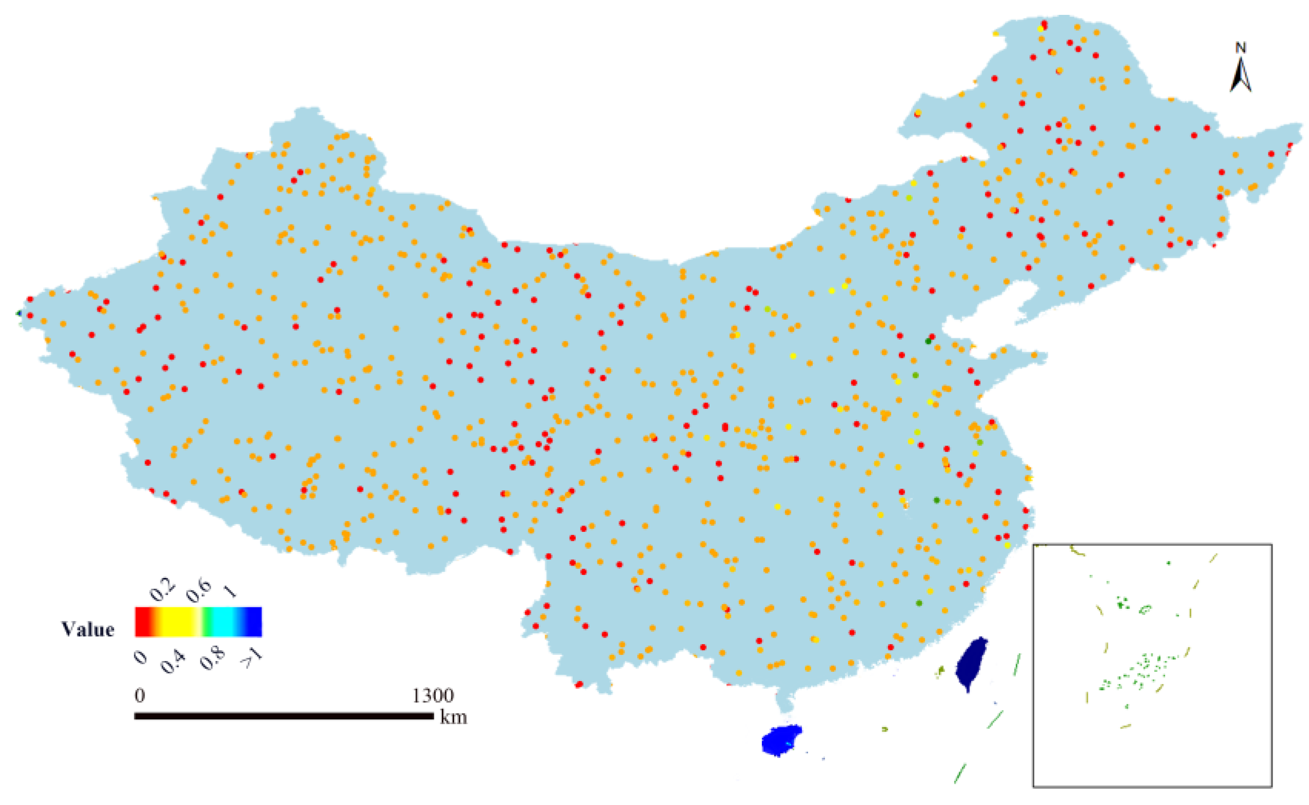
In order to show the spatial distribution of the original precipitation data more intuitively, we superimposed the precipitation data of a selected time step on the geographic base map of China in the form of pixels, as shown in
Figure 1. In the figure, the color brightness is proportional to the precipitation intensity, and the greater the precipitation, the brighter the color of the region.
2.4. Definition
The idea for solving the time series forecasting problem was to mine the potential information and trends embedded in the data by modeling the historical data. The specifics can be described in mathematical form as Equation (1):
where
is a one-dimensional vector containing features and
is inferred value of current time
t within time period
m. The goal is to fit the function
as much as possible with all the data X{
} and Y{
} available in history, so as to infer the value of
y at the next time from the historical data at any time, where
x represents the known precipitation data and
y represents the value of the precipitation data to be predicted.
2.5. Environment Configuration and Model Parameters
This experiment was built on a hardware configuration with 64 GB of RAM and a NVIDIA-RTX5000 GPU, using the Windows 10 operating system, torch version 2.1.0 + cuda121, and pycharm version 2023.2.4 for the experiment.
Table 2 lists the configured hyperparameters.
2.6. DC-CNN-BiLSTM
Traditional LSTM models can only account for unidirectional temporal dependencies in time series, making them less effective for the complex and bidirectional nature of precipitation series. This limitation hampers accurate predictions. To address this, the DC-CNN-BiLSTM model integrates the feature extraction efficiency of the dilation causal convolutional neural network (DC-CNN) with the powerful sequence modeling capabilities of BiLSTM. Additionally, it leverages the unique advantages of a multi-attention mechanism to further enhance prediction accuracy. Due to the organic combination of these three components, the DC-CNN-BiLSTM model can more accurately capture complex dynamics in precipitation data.
Therefore, we propose the DC-CNN-BiLSTM model. As shown in
Figure 2, the DC-CNN-BiLSTM hybrid neural network model constructed in this paper is a prediction model that takes a single feature time series variable as its input and a single variable as its output, and consists of an input layer, a causal convolutional layer, a multi-head attention (Ma) and BiLSTM layer, and an output layer. Among them, the dilatation causal convolution layer realizes the spatial dependence in the context of the input layer, and dilatation expands its vision. A flatten layer and dropout layer were added to optimize the model performance. The fully connected layer (FC-layer) is used to convert the output 2D feature map into a 1D vector. The error feature map is a graph generated using 10*10 errors of four different predictions. N is the batch size, T is the total time step, and E is the size of the embedding.
BiLSTM lacks the ability to learn cross-features and cannot better handle the multidimensional influences in precipitation prediction. And CNNs cannot handle the time series characteristics of precipitation prediction. Considering that CNNs’ strength lies in feature extraction and BiLSTM can effectively handle time series data [
22], in order to take advantage of the two models, the two were combined to form a CNN-BiLSTM neural network model.
2.7. Model Details
Conventional convolutional neural networks typically capture spatial features by processing input data in parallel. However, when handling time series data or tasks with temporal dependencies, standard convolution may fall short in capturing causal relationships within the data. To address this issue, we introduced causal convolutions into neural networks, which incorporate causal dependencies along the time dimension. By introducing null coefficients, causal convolutions also account for dependencies in the spatial dimension. Furthermore, the Bidirectional Long Short-Term Memory network BiLSTM enhances the overall model by tightly integrating temporal and spatial relationships through its time-dependent structure.
2.7.1. DC-CNN for Spatial Dependencies
DC-CNNs, or dilatation causal convolutional neural networks, are obtained by adding an expansion coefficient to causal convolution, thereby increasing the sensory field of the convolutional kernel. The expansion coefficient determines the step size of the convolutional kernel jumps on the input data, allowing the network to efficiently capture long-distance dependencies in the input data without the need to increase the hierarchical depth. CNNs contain multiple feature extractors consisting of convolutional and pooling layers; pooling layers are not included in causal convolution. The general per neuron operation is to apply a linear transformation to the input, followed by a nonlinear function. Mathematically, this can be expressed as follows:
where
denotes the result of each neural network unit operation,
, in which
is the input matrix and
is the weight matrix. A neural network model is formed when multiple units are combined and have a hierarchical structure. Specifically, the main functions of a convolutional neural network are to perform feature extraction on data and capture contextual sequences.
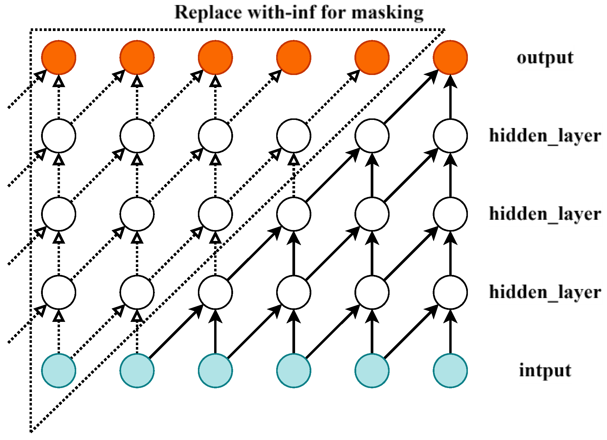
In time series tasks, standard convolution applies the kernel across the entire input, including past, present, and future time steps, which may unintentionally introduce future information. To preserve causality, masking is applied to remove connections from future time steps. Specifically, links from future positions are masked with -inf, causing the softmax operation to assign near-zero attention weights to those positions. Padding is then added to maintain the output size. This approach enables causal convolution, ensuring that the output at each time step depends only on the current and previous inputs, effectively capturing temporal and spatial dependencies. The input layer is a one-dimensional vector, as illustrated in
Figure 3.
The dilation convolutional neural network expands the coverage of the convolution kernel to the historical data on this basis; i.e., the hollow dilation parameter is used during the movement of the convolution kernel to expand the coverage of the convolution kernel. In dilation convolution, a void coefficient (dilation rate) is inserted into the convolution kernel to expand the sensory field of the convolution kernel. The DC-CNN structure diagram after adding a dilation mechanism, when the input is a one-dimensional vector, is shown in
Figure 4.
It can be observed that, after accounting for dilation convolution, the next layer of neurons in the causal neural network has a significantly enlarged field of view for sensing the historical information of the neurons in the previous layer. Through the mechanism of dilation, the current causal neural network can then expand the receptive field of view of the causal convolutional network by changing the size of the convolutional kernel (kernel_size) or increasing the dilation parameter while the number of hidden layers remains unchanged. Padding = (kernel_size-1)*dilation was chosen in this paper, and dilation was set to 2. Thus, the embedding process used causal and dilation convolution to capture the context and obtain the spatial relationship of the input data. Then, the context data were passed into the BiLSTM model using a tanh activation function.
2.7.2. Ma-BiLSTM for Contextual Temporal Dependencies
An Ma-BiLSTM is a Bidirectional Long Short-Term Memory network with the addition of multi-head attention mechanism. The multi-head attention mechanism was added in the class initialization stage, and the context data captured by causal convolution are imported. After adjusting the dimensional order of the processed data in the causal convolution, the weights continue to be adjusted by the multi-head attention mechanism.
LSTM is a variant of a Recurrent Neural Network which utilizes the logical control of gate units to realize the operation of data. BiLSTM adds three gating structures in the hidden layer h, which are a forget gate, input gate, and output gate, and also adds a hidden state [
23].
,
, and
denote the values of the forget gate, input gate, and output gate at moment t, respectively;
is the input value at the moment t;
is the output value of the hidden layer at the current moment;
is the state information at the current moment; and
σ is the sigmoid activation function.
The forgetting gate determines the extent to which the cell state of the previous moment is retained in the current moment. Its output
is represented by Equation (3):
The input gate determines the extent to which the input
of the network at the current moment is saved to the cell state
, and its output
is represented by Equation (4):
In Equations (3) and (4),
and
denote the weight matrices of the forgetting gate and the input gate, respectively, and
and
denote the bias terms of the forgetting gate and the input gate, respectively.
is used to characterize the state of the current input unit and is represented as follows:
The memory unit is used to compute the cell state
at the current moment,
is represented by the sum of the cell state
at the previous moment multiplied by element by the forgetting gate
, and the current input cell state
multiplied by element by the input gate
:
By Equation (6), the BiLSTM model’s memory about the current moment and its long-term memory are then associated in order to form a new memory .
In Equations (5) and (6), is the weight matrix of the memory cell and is the bias term of the memory cell.
The output gate controls the effect of long-term memory on the current output, which is processed by a sigmoid function to obtain the output
of the unit:
The hidden layer output
is jointly determined by the output gate and the new cell state:
In Equations (7) and (8), is the weight matrix of the output gate and is the bias term of the output gate.
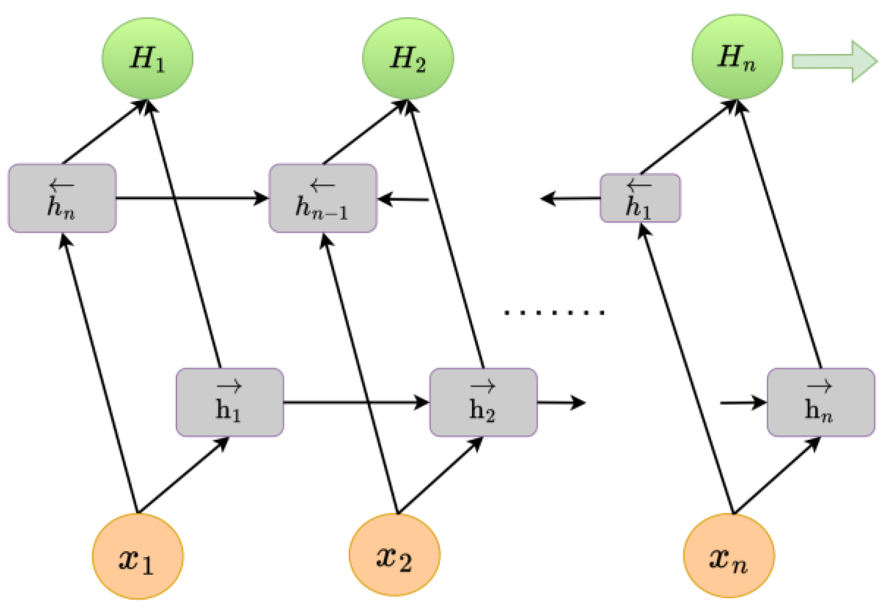
Figure 5 shows the BiLSTM neural network structural model; its structure is similar to that of an LSTM.
is the input to the network at the current moment,
is the output of the hidden layer, and
is the final feature expression obtained by splicing the positive-order and reverse-order outputs with
∈ [1,
].
is the eventually hidden state at the current moment,
, and the output fully connects all hidden states. BiLSTM is optimized on the basis of LSTM; the BiLSTM neural network structure model is composed of two independent LSTM modules, and their input sequences are fed into the two LSTM neural networks in positive and reverse order for feature extraction, respectively. The parameters of the two LSTM neural networks in BiLSTM are independent of each other, and they only share the word-embedding word vector list. BiLSTM predicts precipitation using time series within time steps, rather than being validated against future predicted precipitation.
The resulting DC-CNN-BiLSTM model combines the strengths of the DC-CNN and the Ma-BiLSTM network, creating a hybrid model.
2.8. Loss Function
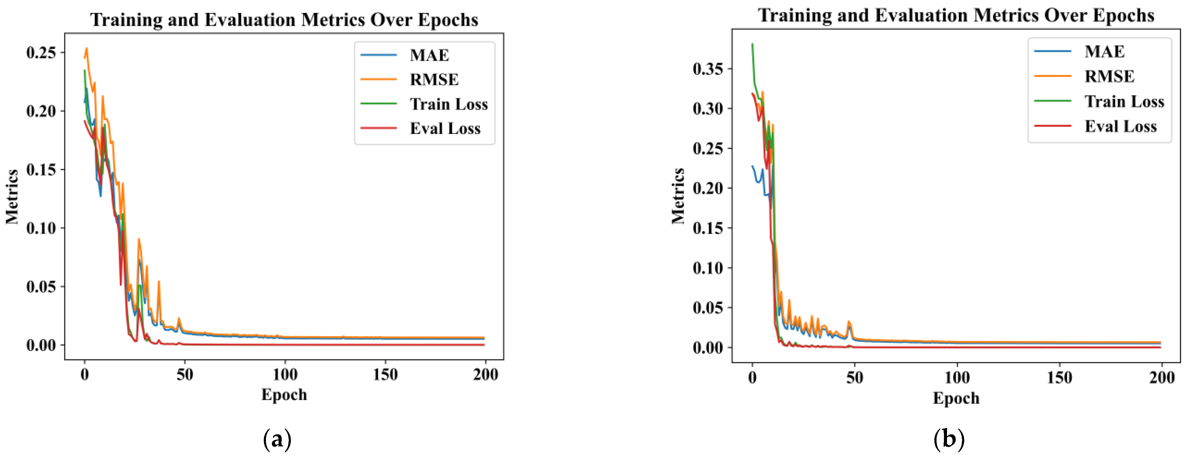
In the whole prediction model, the Mean Squared Error (MSE), Root Mean Squared Error (RMSE), and Mean Absolute Error (MAE) were selected to calculate the error loss. Loss is evaluated using MSE at Train Loss and Eval Loss, and RMSE at validation. Mean Squared Error refers to the expected value of the squared difference between the estimated value of a parameter and the true value of the parameter, which can evaluate the degree of change in the data and is denoted as
. RMSE is the square root of the Mean Squared Error, which more intuitively represents the average error between the predicted values and the actual values, denoted as
. Compared to RMSE, MAE is relatively less sensitive to outliers, easier to interpret, and consistent with the units of the original data. In these two indicators, the smaller the value is, the more accurate the prediction of the model is. The formula is as follows.
In Equations (9) and (10), and denote the normalized predicted and true values, respectively, and is the total number of samples.
2.9. Model Building
In this study, a hybrid prediction model based on a DC-CNN, BiLSTM, and a multi-head attention mechanism was proposed. In the process of model construction, firstly, the multi-scale long-term dependence features of the input sequence were extracted through the dilated causal convolution structure of the DC-CNN module (the inflation factor was 20 to 22). Then, the high-level features output by the DC-CNN were input into the BiLSTM module to synchronously capture the history and future potential dynamic association through bidirectional time series modeling. In order to further enhance the utilization efficiency of key temporal information, a multi-head attention mechanism was introduced in front of the BiLSTM module to dynamically calculate the weight distribution of different time steps to focus on important signal segments.
The DC-CNN-BiLSTM model utilized Adam optimization with tanh and sigmoid activation functions, combined with Dropout regularization (0.5 rate), to mitigate overfitting. Training proceeded through sequential phases: forward propagation computed predictions and cross-entropy loss, followed by backpropagation deriving parameter gradients via automatic differentiation. These gradients then guided weight updates using Adam’s adaptive learning rates and momentum-based adjustments, iteratively minimizing prediction errors while maintaining model generalization through controlled parameter stochasticity and gradient-directed optimization. To evaluate the performance of the hybrid model, a random hierarchical partitioning strategy was adopted to divide the data into a training subset and a test subset. The training set was used to train the model, while the test set was used to evaluate the generalization ability of the model. During this process, the data were divided into k subsets, and the model was trained and tested on different combinations of these subsets to evaluate its performance more comprehensively. The final model performance was averaged over multiple runs to ensure stability and universality.
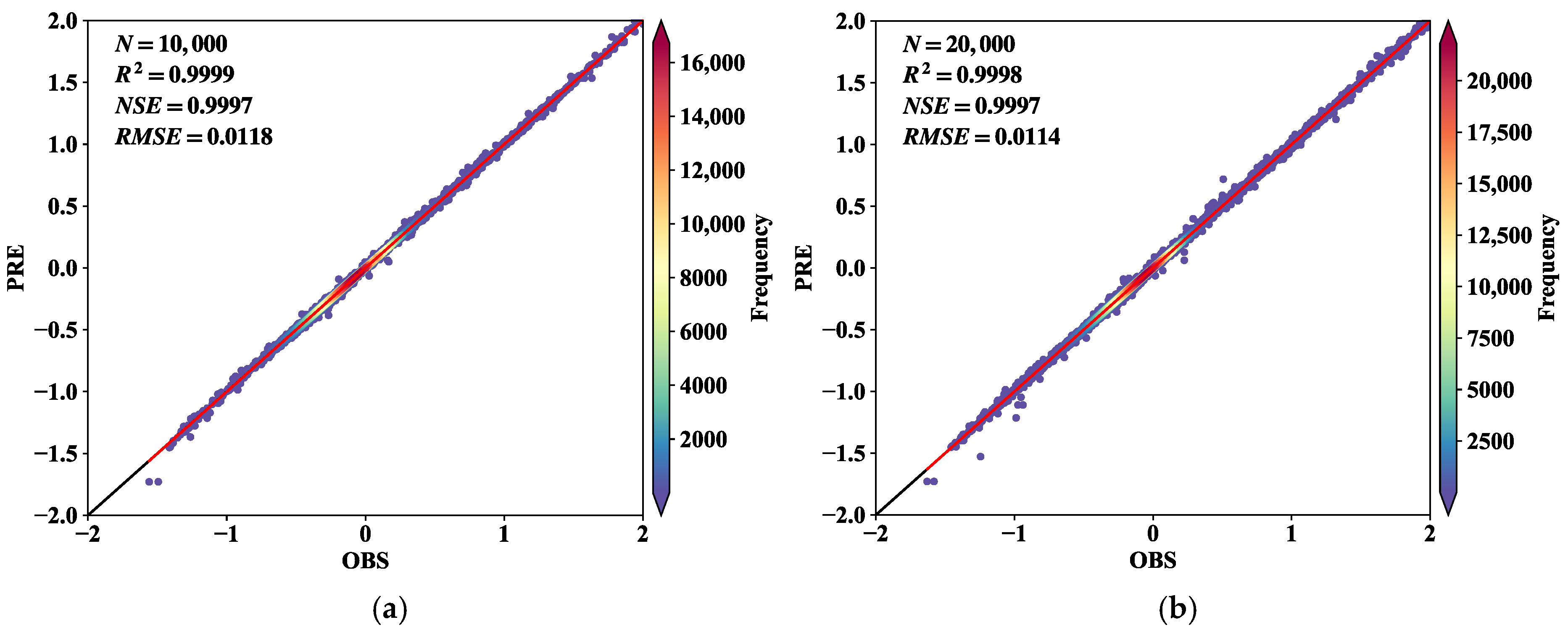
The performance of the model was evaluated using several key evaluation indicators. The Mean Absolute Error (MAE) was used to visually measure the magnitude of the prediction error. The Root Mean Square Error (RMSE) was chosen because of its sensitivity to large errors, as it can penalize large deviations between predicted values and actual values. The Mean Squared Error (MSE) was used as a loss function in training to calculate the average square difference between the predicted values and the actual values, providing a sense of the accuracy of the model. Finally, the coefficient of determination (R2) was used to quantify the extent to which the model explained the variance in the target variable. The higher the R2, the better the overall fit.
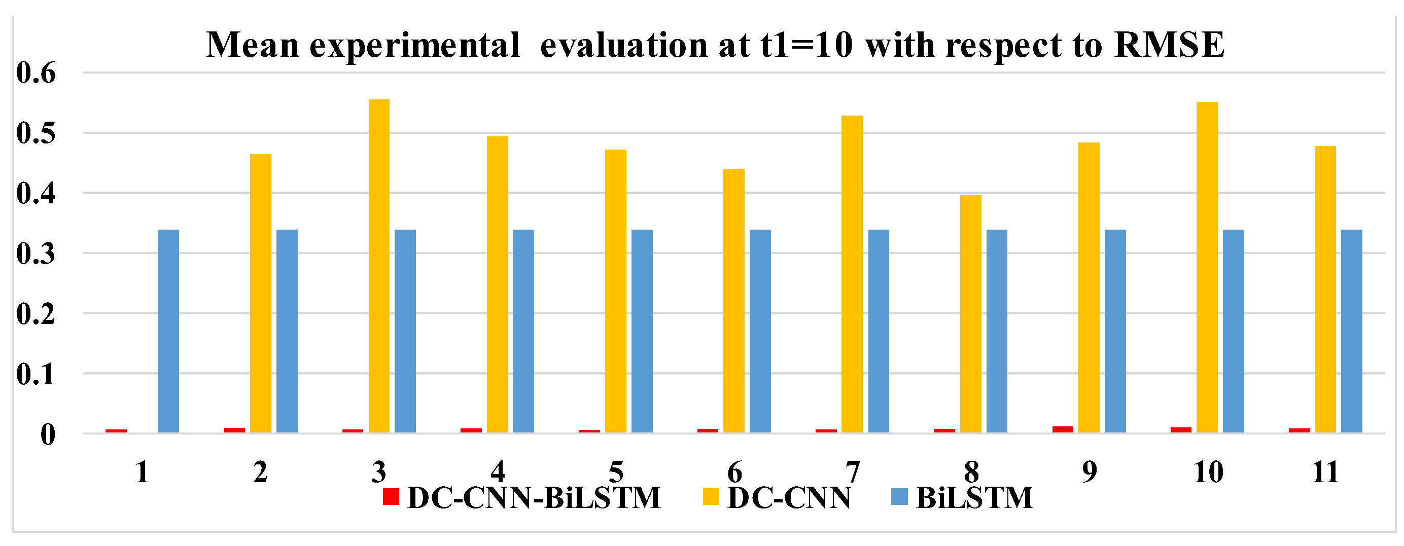
Ablation studies were conducted to evaluate the contribution of each module in the model. In this study, the DC-CNN and Ma-BiLSTM modules were removed one by one to evaluate their individual influences on the model performance. In the first variant, the DC-CNN module was removed and only BiLSTM was used to evaluate the model. In the second variant, the BiLSTM module was excluded, leaving DC-CNN and the attention mechanism. The same MAE and RMSE were used to measure the influence of each indicator on each module.
4. Discussion
Understanding the intrinsic spatio-temporal characteristics of precipitation is essential for the accurate prediction model in this paper. The spatio-temporal distribution characteristics of precipitation in this paper are essentially driven by complex meteorological processes, which means that the model must capture both their long-range dependence over time and cooperative variation in space. Previous studies have shown that precipitation series exhibit weak but significant long-range dependence in the temporal dimension, which is particularly prominent in extreme precipitation events and is enhanced with an increase in spatial aggregation scale [
28,
29,
30]. This temporal persistence may be related to low-frequency oscillations in atmospheric circulation, such as the ENSO cycle, or the inertia of regional water vapor transport. At the same time, the spatial dependence of daily precipitation has been widely confirmed [
31].
The DC-CNN-BiLSTM model shows significant advantages. Firstly, by introducing a Deep Convolutional Network (DC-CNN), the model can extract rich spatial local features from the original precipitation data and effectively identify the spatial distribution structure of heavy precipitation regions. At the same time, combined with the time-modeling ability of BiLSTM, the model can capture long-distance time dependencies, so as to describe the precipitation evolution process more accurately.
Although DC-CNN-BiLSTM has some effect, the model has certain limitations and areas for future improvement. Firstly, the dataset used in this study is limited in terms of precipitation attributes, containing only basic meteorological data. It does not incorporate other potential influencing factors, such as barometric pressure, wind speed, and humidity, which may restrict further improvements in prediction accuracy. This approach may place excessive reliance on statistical features in the data rather than capturing the underlying physical mechanisms. Consequently, despite the model’s high performance, its predictive physical consistency and reliability may be compromised when applied to extreme climate conditions or unconventional scenarios. Future work could enhance the interpretability and reliability of the model by incorporating additional meteorological variables or integrating methods with physical constraints, such as Das [
32], who employ a hybrid physics–AI framework analogous to PINNs, integrating atmospheric dynamics equations with observational radar/satellite data to improve extreme precipitation nowcasting accuracy, particularly for short-term, high-intensity rainfall events.
Furthermore, there are uncertainties associated with the model performance, particularly in situations involving data distribution shifts or extreme climate scenarios not well represented in the training data. These uncertainties stem from both data limitations and the inherent complexity of atmospheric systems, which are not fully captured by data-driven models.
In addition, the performance of the model when dealing with high-frequency and low-frequency precipitation events also needs to be optimized. The current model still has a certain deviation in the prediction of extreme weather events, because too-low or too-high precipitation values for extreme weather will affect the overall precipitation prediction, and very few weather data make the prediction of extreme weather inaccurate. This is also part of the reason why the model’s RMSE values are generally higher than its MAE results. The model is also susceptible to issues such as gradient disappearance and gradient explosion.
5. Conclusions
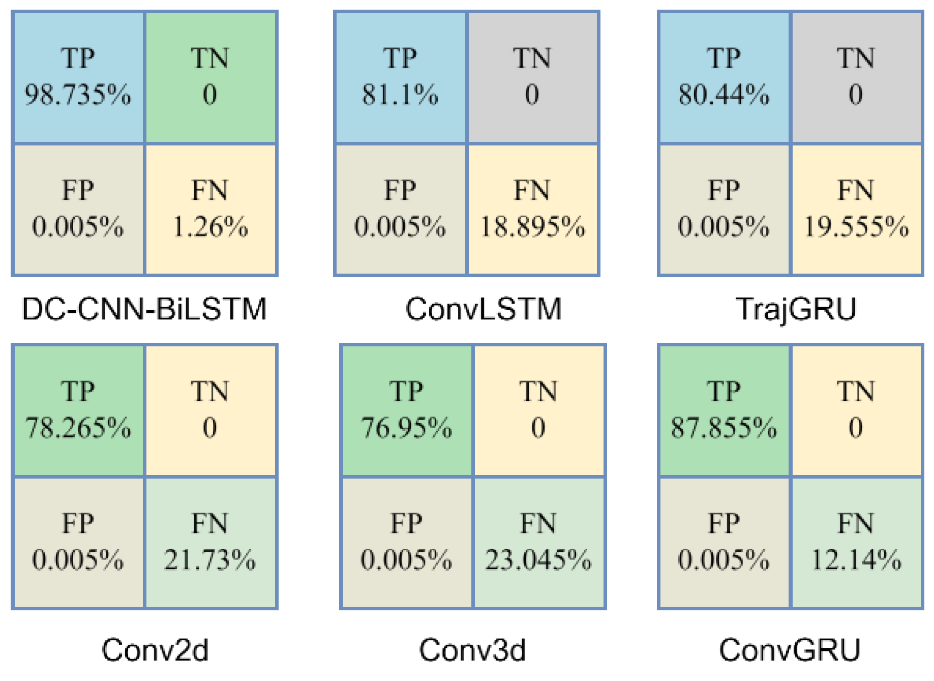
In this paper, we introduced the DC-CNN-BiLSTM model, a deep learning-based approach designed to overcome the limitations of other deep learning-based precipitation prediction methods, such as ConvLSTM and ConvGRU, in understanding regional meteorological dynamics and forecasting weather events. By integrating a DC-CNN and BiLSTM, the model effectively captures both spatial and temporal dependencies, significantly enhancing precipitation forecasting accuracy. Our experimental results demonstrate that the proposed framework outperforms traditional methods, maintaining stable predictive performance and reducing forecast errors, particularly in medium–long-time-period precipitation scenarios. These findings underscore the model’s innovative contribution to advancing deep learning applications in meteorology.
Future research should focus on expanding the model’s capability by incorporating additional precipitation attributes to construct a more comprehensive multi-dimensional feature space. Enhancing the model’s structure will be crucial for better handling precipitation events with varying frequencies, while further optimizing the self-attention mechanism could improve prediction accuracy. Additionally, integrating advanced deep learning techniques, such as gradient penalty methods, can further enhance the model’s robustness and generalization ability.
Beyond technical advancements, this research holds significant implications for policy. More accurate precipitation forecasts can improve disaster preparedness, optimize water resource management, and support climate adaptation strategies. By strengthening predictive capabilities, this study contributes to the development of more resilient meteorological forecasting systems, aiding policymakers in mitigating the impact of some extreme weather events and enhancing long-term climate risk management.
Overall, the impressive performance of the DC-CNN-BiLSTM model in precipitation prediction highlights the significant potential of deep learning in weather forecasting. Future research should focus on further optimizing the model structure, incorporating additional meteorological data, and enhancing the model’s generalization ability and prediction accuracy. These efforts will contribute to developing a more comprehensive solution for addressing the complexities and dynamics of the ever-changing meteorological environment.


