A Comparative Study of a Two-Dimensional Slope Hydrodynamic Model (TDSHM), Long Short-Term Memory (LSTM), and Convolutional Neural Network (CNN) Models for Runoff Prediction

Abstract

Accurate runoff prediction in complex slope catchments remains challenging due to terrain heterogeneity and dynamic rainfall interactions. This study conducts a systematic comparison between a physics-based Two-Dimensional Slope Hydrodynamic Model (TDSHM) and data-driven deep learning models (LSTM and CNN) for runoff forecasting under variable rainfall conditions. Using 214 rainfall–runoff events (2013–2023) from the Qiaotou watershed in Nanjing, China, the TDSHM integrates rainfall momentum, wind effects, and hydrodynamic principles to resolve spatiotemporal flow dynamics, while LSTM and CNN models leverage seven hydrological features for data-driven predictions. Results demonstrate that the TDSHM achieved superior accuracy, with a mean relative error of 10.77%, Nash–Sutcliffe Efficiency (NSE) of 0.801, and Mean Absolute Error (MAE) of 3.17 mm, outperforming LSTM (24.38% error, NSE = 0.751, MAE = 4.61 mm) and CNN (28.10% error, NSE = 0.506, MAE = 6.82 mm). The TDSHM’s explicit physical interpretability enabled precise simulation of vegetation-modulated runoff processes, validated against field observations (92% predictions within ±15% error). While LSTM captured temporal dependencies effectively, CNN exhibited limitations in sequential data processing. This study highlights the TDSHM’s robustness for scenarios requiring mechanistic insights and the complementary role of LSTM in data-rich environments. The findings provide critical guidance for flood risk management, soil conservation, and model selection trade-offs between physical fidelity and computational efficiency.

1. Introduction

The prediction models for slope runoff can be broadly categorized into two types: data-driven models and process-driven models [1,2]. Data-driven models utilize historical data patterns to predict runoff, effectively mitigating uncertainties inherent in physical assumptions, which explains their widespread adoption in hydrological forecasting [3,4,5]. Recent advancements in machine learning—a cornerstone of data-driven modeling—have revolutionized hydrological prediction capabilities [6,7]. Notably, Shortridge et al. [8] demonstrated scenarios where data-driven models outperform traditional physical models in predictive accuracy. Empirical studies by Su et al. [9] and Liang et al. [10] revealed that support vector regression (SVR) and support vector machines (SVM) exhibit exceptional performance in watershed-scale runoff prediction, particularly under data-abundant and highly predictable conditions. Long Short-Term Memory (LSTM) networks have emerged as particularly powerful tools for hydrometeorological simulations, achieving remarkable precision in short-term runoff forecasting [11,12,13]. Guo et al. [14] and Tian et al. [15] further substantiated LSTM’s capacity to decode complex temporal patterns, thereby enhancing prediction reliability. In contrast, process-driven models prioritize the mechanistic understanding of hydrological processes through 1D/2D slope runoff simulations, with particular emphasis on spatiotemporal water flow dynamics [16,17,18]. While Saint-Venant equations remain fundamental in slope runoff modeling, their application to steep terrains suffers from accuracy degradation and prohibitive computational demands [19,20]. This has spurred development of simplified approaches like kinematic wave and diffusion wave models, which balance computational efficiency with acceptable accuracy [21,22]. However, existing frameworks by Cai et al. [23] and Shi et al. [24], despite incorporating slope variability and net rainfall intensity fluctuations, overlook critical factors like rainfall momentum and wind effects. Practical challenges arise from terrain heterogeneity, where conventional 1D models prove inadequate, necessitating 2D simulation frameworks. Lan et al. [25] advanced this field through coupling Saint-Venant and Richards equations in the Tsinghua hillside runoff model, enabling multi-hydrodynamic process simulation. Parallel innovations by Yu et al. [26] introduced terrain-adaptive Saint-Venant equation variants, providing novel solutions to these complex hydrological challenges.

Despite significant advancements in slope runoff prediction, critical challenges persist in balancing physical fidelity and computational efficiency. While traditional two-dimensional hydrodynamic models historically faced limitations in simulating complex slope catchments, recent innovations in high-performance computing have expanded their applicability. Pasculli et al. [27] demonstrated that GPU-accelerated shallow water models can achieve Nash–Sutcliffe efficiency (NSE) >0.85 for dynamic flood forecasting in steep Mediterranean basins, though such approaches often oversimplify vertical hydrological processes like wind-driven rainfall redistribution [28]. Meanwhile, deep learning methods, while excelling at capturing nonlinear rainfall–runoff relationships [29], face scalability constraints at the watershed scale—particularly in large catchments (>500 km²), where sparse monitoring networks exacerbate data scarcity and sensor noise [30]. A key challenge lies in systematically comparing and selecting between hydrodynamic simulations and deep learning approaches to enhance model accuracy and expand applicability.

This study aims to evaluate the performance of a two-dimensional slope hydrodynamic model (TDSHM) and deep learning models in predicting runoff for complex slope catchments under variable rainfall conditions. Utilizing long-term monitoring data from the Qiaotou watershed in Nanjing’s Lishui District, we first establish and validate a hydrodynamic model. Subsequently, we apply LSTM and CNN models for runoff prediction, comparing the accuracy and applicability of both methods (The experimental procedure is shown in Figure 1). The findings have significant practical implications for mitigating flood risks, controlling soil erosion, and optimizing agricultural water management. Precise runoff predictions can offer a scientific foundation for water resource allocation, irrigation scheduling, and policy development [31,32,33].

2. Research Area and Data

2.1. Study Area Overview

The Qiaotou experimental watershed (32°06′ N, 141°40′ E; 3.1 km²) represents a critical headwater catchment in the Qinhuai River system of the lower Yangtze Basin (The exact location is shown in Figure 2). This benchmark site, established in 2011 under China’s National Soil Conservation Monitoring Network (Code: FA3220614140), features a complete rainfall–runoff monitoring system collecting 30 min resolution data since 2013 (MWR, 2015). The watershed’s geomorphic characteristics include (1) elevation gradients from 220 m (NE) to 30 m (SW) with low-mountain/hill terrain; (2) dominant red–brown soils (pH 4.6–5.8, depth < 50 cm) exhibiting high erodibility (K factor > 0.35); and (3) a humid subtropical climate with mean annual precipitation of 1107 mm (75% occurring May–September) and temperature of 15.5 °C.

As the principal headwater of the Lishui Ergan River (Qinhuai River tributary), draining into Fangbian Reservoir, the watershed’s compact scale enables effective separation of anthropogenic impacts (e.g., reservoir operations caused 18% runoff variation in 2016–2020) from natural hydrological processes. Our research framework, validated through process-based modeling using the high-resolution dataset, will be extended to mesoscale basins (>500 km²) in the Yangtze mid-lower reaches to address spatial scaling challenges in erosion-prone subtropical catchments.

2.2. Data

The study utilized data from the Soil Erosion Dynamic Monitoring Station (Station ID: FA3220614140) located in the Qiaotou Watershed, Lishui District, Nanjing City, Jiangsu Province (119°10′05″ E, 31°40′28″ N). The monitored area comprises red–brown soil with a bulk density of 1.13 g/cm³. Five standardized slope runoff plots were established, each measuring 5 m (width) × 10 m (length) with a 9° inclination. A rectangular collection ditch (0.25 m wide × 0.20 m deep, 1% slope) was installed at the base of each plot, followed by two sedimentation pools. Post-rainfall measurements included diversion bucket depth to calculate total runoff volume. Homogenized samples were oven-dried to determine sediment concentration, enabling soil loss quantification.

Meteorological data were obtained from adjacent weather stations and automated sensors maintained by the Nanjing Hydraulic Research Institute. The rainfall data were collected using an SL3.1 tipping bucket rain gauge (Tianjin Weather Equipment Inc.) with a measurement accuracy of 0.1 mm, which complies with the World Meteorological Organization (WMO) precipitation measurement standards (WMO No. 8, 2018).

Runoff monitoring followed WMO hydrological observation guidelines: The runoff volume was quantified using the volumetric method through a V-notch weir (Type 12-H/WS, accuracy ±5%) installed at the watershed outlet. The sediment concentration was determined by homogenizing the sediment–water mixture in the tank, transferring it to sampling bottles, and subsequently measuring it using the drying method (105 °C for 24 h). Rainfall–runoff relationships were statistically validated (The calculation method is shown in Equation (1)), showing a strong power-law correlation between total precipitation (P) and runoff depth (H):

$$\mathrm{H}=0.87{\mathrm{P}}^{1.12}\left({\mathrm{R}}^2=0.91,\mathrm{p}<0.001\right)$$

(1)

Events were classified as independent if separated by >6 h dry intervals, with the antecedent precipitation index (API) < 5 mm.

Analysis of 2013–2023 monitoring records (n = 214) focused on eight rainfall parameters (The detailed information is presented in

Table 1. Descriptive statistical characteristics of rainfall events.

Parameters	Minimum Value	Maximum Value	Mean	Standard Deviation
P	0.50	286.00	40.55	40.02
T	5.00	4565.00	952.97	771.06
I	0.40	306.00	6.67	22.69
I30	0.50	130.91	21.56	19.56
R	0.08	4661.18	312.35	568.95
Qmax	0.01	88.00	4.56	10.04
K	0.01	17.60	0.45	1.48
H	0.02	147.80	10.21	24.17

): total precipitation (P, mm), total rainfall time (T, min), maximum 30 min intensity (I₃₀, mm/h), mean intensity (I, mm/h), erosion intensity (R, t/(km²·a)), peak flow (Q_max, m³/s), runoff coefficient (K), and runoff depth (H, mm). Statistical methods encompassed descriptive analysis and Pearson correlation, with all variables passing the Kolmogorov–Smirnov normality test (p > 0.15).

2.3. Data Preprocessing

The raw dataset comprised 214 rainfall–runoff events with eight variables: precipitation (P), total rainfall time (T), maximum 30 min rainfall intensity (I₃₀), total rainfall (I), erosion intensity (R), peak discharge (Q_max), runoff coefficient (K), and runoff depth (H). The preprocessing workflow consisted of three sequential steps: data cleaning, missing value interpolation, and normalization.

1. Data Cleaning

Data cleaning eliminates noise, outliers, and irrelevant information to enhance model generalizability [34,35]. The procedure involved:

• Missing value detection: temporal gaps in time series data may disrupt temporal dependency learning, necessitating systematic identification of incomplete records.
• Outlier treatment: anomalous values arising from measurement errors or data entry inconsistencies were detected and corrected using the Z-score method (threshold: |Z| > 3) [36,37].
• Noise reduction: a moving average filter with a 3-point window was applied to smooth stochastic fluctuations in time series variables while preserving trend patterns [38].

2. Missing Value Interpolation

Linear interpolation was employed to reconstruct missing data points by fitting a piecewise linear function between adjacent valid observations. This method assumes temporal continuity of hydrological variables, enabling robust estimation of unrecorded values through the Equation (2):

$${\mathrm{x}}_{\mathrm{t}}^{\prime }={\mathrm{x}}_{\mathrm{t}-1}+{\displaystyle \frac{\left({\mathrm{x}}_{\mathrm{t}+1}-{\mathrm{x}}_{\mathrm{t}-1}\right)}{2}}$$

(2)

where $x_t^{\prime }$ represents the interpolated value at time t.

3. Normalization

Feature scaling via min–max normalization transformed all variables to a [0, 1] range using Equation (3) [39]:

$$x_{norm}={\displaystyle \frac{x-x_{min}}{x_{max}-x_{min}}}$$

(3)

This standardization mitigates feature magnitude disparities, accelerating model convergence and improving prediction stability. Post-prediction inverse normalization restored outputs to original physical units for interpretability.

2.4. Selection of Feature Parameters

To investigate inter-parameter correlations, we constructed a Pearson correlation coefficient matrix using MATLAB 2023b (the detailed information is presented in Figure 3). Based on established hydrological study standards, the correlation strengths were classified as strong (0.5–0.9), moderate (0.2–0.5), and weak/negligible (<0.2). The matrix revealed distinct correlation patterns between runoff volume (H) and seven candidate parameters:

• Runoff Coefficient (K) and H: 0.586
• Peak Discharge (Q_max) and H: 0.508
• Total Precipitation (P) and H: 0.488
• Maximum 30 min Rainfall Intensity (I₃₀) and H: 0.452
• Total Rainfall Time (T) and H: 0.368
• Rainfall Erosivity (R) and H: 0.341
• Average Rainfall Intensity (I) and H: 0.322

The parameter influence hierarchy emerged as K > Q_max > P > I₃₀ > T > R > I, based on descending correlation magnitudes. Following the principles of hydrological parameter selection (including measurement sensitivity, temporal stability, parameter independence, and data accessibility), we ultimately incorporated seven key parameters into the prediction model: T, P, I, I₃₀, R, Q_max, and K. These parameters demonstrate established sensitivity to regional soil erosion dynamics, according to domestic watershed studies. Runoff depth (H) was designated as the model’s output variable, completing the framework for runoff generation modeling.

2.5. Validation Set Samples

From the 214 recorded runoff-producing events, 15 representative rainfall episodes were systematically selected for validation of both the 2D slope hydrodynamic model and machine learning models. The key characteristic parameters of these events are comprehensively tabulated in

Table 2. Main characteristic parameters of test samples.

No.	Rainfall Date	Rainfall (mm)	Rainfall Intensity (mm/h)	Rain Type
1	2014.05.11	18.00	1.430	Moderate rain
2	2014.08.29	45.00	5.745	Heavy rain
3	2015.08.10	78.50	2.201	Torrential rain
4	2015.05.15	69.60	6.692	Torrential rain
5	2016.05.02	9.50	4.839	Light rain
6	2016.07.07	77.5	32.07	Torrential rain
7	2016.10.28	6.00	0.480	Light rain
8	2017.06.10	145.00	7.945	Extraordinarily torrential rain
9	2017.10.14	6.00	1.029	Light rain
10	2018.09.17	37.00	2.581	Heavy rain
11	2019.08.28	13.50	1.080	Moderate rain
12	2019.09.02	39.50	2.184	Heavy rain
13	2020.06.15	146.50	15.287	Torrential rain
14	2020.09.11	35.00	3.043	Heavy rain
15	2021.06.03	34.00	0.895	Heavy rain

.

3. Methods

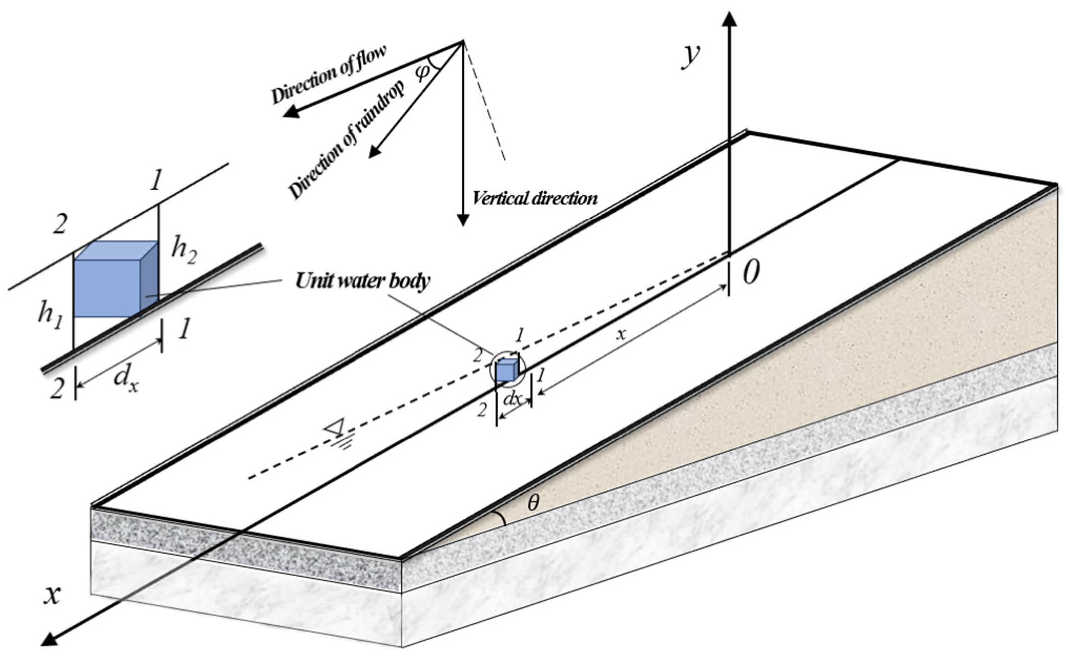
3.1. Two-Dimensional Slope Hydrodynamic Simulation Model (TDSHM)

The Saint-Venant equation, as the core control equation describing the mechanism of slope flow, is widely applied in the simulation research of hydrological processes on slopes. Based on this equation framework, this study has improved and established a runoff prediction mechanism model that couples the effects of soil and water conservation measures under natural rainfall conditions, achieving dynamic simulation and prediction of slope runoff processes under different control measures. Consider water flow moving along a sloped bed inclined at angle θ. A Cartesian coordinate system is defined such that the x-axis aligns with the slope direction, while the y-axis is perpendicular to it (the detailed information is presented in Figure 4). Let the wind-adjusted terminal velocity of raindrops impacting the water surface be denoted as $v_{\mathrm{m}}\left(x,t\right)$, with an inclination angle φ relative to the flow direction. The slope is modeled as a unit–width prismatic channel. Two adjacent cross-sections (1–1 and 2–2), separated by a differential distance dx, are selected to form a control volume. The continuity and momentum equations are formulated along the x-axis.

1. Derivation of momentum equation. Based on the fundamental principles of fluid dynamics, we propose a physically based model that couples mass and momentum conservation to characterize runoff generation and concentration on hillslopes under natural rainfall conditions. By systematically formulating one-dimensional governing equations for overland flow, we establish motion and continuity equations applicable to a broad range of slope angles (0°–90°). The model integrates the effects of rainfall kinetic energy input, slope-induced resistance, and aerodynamic drag forces to comprehensively describe the hydrodynamic processes governing hillslope overland flow dynamics as shown in Equation (4).

$${\displaystyle \frac{\partial u}{\partial t}}+u{\displaystyle \frac{\partial u}{\partial x}}+g{\displaystyle \frac{\partial h}{\partial x}}=g\left(S_0-S_f\right)-{\displaystyle \frac{\sigma }{\rho h}}+{\displaystyle \frac{p\left(x,t\right)}{2h}}{v}_m\left(x,t\right)\sin 2\phi -{\displaystyle \frac{i\left(x,t\right)}{h}}u\sin \phi$$

(4)

2. Derivation of continuity equation. For an incompressible thin layer of water flow on a hillslope, the continuity equation describing the overland flow can be derived by simplifying the water balance equation for an elemental volume over a time interval as shown in Equation (5).

$${\displaystyle \frac{\partial h}{\partial t}}\mathrm{d}x\mathrm{d}t=\left[\begin{array}{c}i\left(x,t\right)\cos \left(90°-\phi \right)\mathrm{d}x\mathrm{d}t+uh\mathrm{d}t\end{array}\right]-\left[\begin{array}{c}uh+{\displaystyle \frac{\partial \left(uh\right)}{\partial x}}\mathrm{d}x\end{array}\right]\mathrm{d}t$$

(5)

3. Development of one-dimensional hillslope overland flow equations incorporating variable rainfall intensity, momentum, and wind effects. For short-duration rainfall–runoff events, evaporation and thermal effects were excluded from the governing equations, based on their secondary influence relative to rainfall intensity dynamics and antecedent soil moisture conditions. Neglecting evaporation and temperature factors during rainfall events, we derive governing equations for one-dimensional hillslope overland flow that explicitly account for spatiotemporal variations in rainfall intensity, raindrop momentum, and aerodynamic forcing. The modified Green–Ampt (G-A) infiltration model by Chu [40] is implemented to accommodate dynamic rainfall inputs, enabling robust simulations across diverse precipitation regimes. Key modeling steps include (1) Ponding Condition Analysis: evaluating surface ponding initiation/cessation at rainfall start/end times using G-A-based threshold criteria. (2) Infiltration Dynamics: computing time-dependent infiltration rates through iterative G-A model solutions. (3) Raindrop Terminal Velocity: adopting the semi-analytical approach of Wu et al. [41] and Mou et al. [42] to determine wind-adjusted raindrop impact velocities $v_m\left(x,t\right)$.

The final coupled system of mass–momentum conservation equations is expressed as as shown in Equation (6):

$$\begin{array}{l}{\displaystyle \frac{\partial u}{\partial t}}+u{\displaystyle \frac{\partial u}{\partial x}}+g{\displaystyle \frac{\partial h}{\partial x}}=g\left(S_0-S_f\right)-{\displaystyle \frac{\sigma }{\rho h}}+{\displaystyle \frac{p\left(x,t\right)}{2h}}{v}_a\left(x,t\right)\sin 2\phi -{\displaystyle \frac{i\left(x,t\right)}{h}}u\sin \phi \hfill \\ {\displaystyle \frac{\partial h}{\partial t}}+u{\displaystyle \frac{\partial h}{\partial x}}+h{\displaystyle \frac{\partial u}{\partial x}}=i\left(x,t\right)\sin \phi \hfill \\ i\left(x,t\right)=p\left(x,t\right)-C\left(t\right)-f\left(x,t\right)\hfill \\ v_m\left(x,t\right)=V_m\left(x,t\right){\left[1-\left(1-{\eta }^2\right)\exp \left(-2gHp{V}_m^2\left(x,t\right)\right)\right]}^{p2}\hfill \end{array}$$

(6)

4. Numerical solution of two-dimensional slope hydrodynamic numerical simulation model. To solve Equation (6) numerically, we employ the widely used Preissmann implicit scheme [43,44] in the computation of unsteady open channel flow. The governing partial differential equations, comprising the coupled momentum conservation equation (Equation (4)), slope flow continuity equation (Equation (5)), and the modified Green–Ampt infiltration equation (part of Equation (6)), form the basis of the TDSHM. These equations were implemented and solved numerically using custom code developed in MATLAB (version R2023b). We employed the Preissmann implicit finite difference scheme, a widely used method for unsteady open channel flow, to discretize and solve the coupled equations. After linearization, the scheme results in the system of algebraic equations shown in Equation (7), which are solved iteratively for each time step across the spatial domain.

$$\{\begin{array}{l}{A}_{1j}\mathsf{\Delta }{u}_j+B_{1j}\mathsf{\Delta }{h}_j+C_{1j}\mathsf{\Delta }{u}_{j+1}+D_{1j}\mathsf{\Delta }{h}_{j+1}=E_{1j}\hfill \\ A_{2j}\mathsf{\Delta }{u}_j+B_{2j}\mathsf{\Delta }{h}_j+C_{2j}\mathsf{\Delta }{u}_{j+1}+D_{2j}\mathsf{\Delta }{h}_{j+1}=E_{2j}\hfill \end{array}$$

(7)

Equation (7) forms a set of two nonlinear algebraic equations with four independent unknowns, $\mathsf{\Delta }{u}_j,\mathsf{\Delta }{h}_j,\mathsf{\Delta }{u}_{j+1},\mathsf{\Delta }{h}_{j+1}$, which are common to any two adjacent cross-sections. When the slope is divided into N sections, for each section j (1 ≤ j ≤ N), two similar equations can be written, and there are 2N such equations, together with two boundary condition equations for the slope inlet and outlet, the unique solution of 2(N + 1) unknowns can be solved.

3.2. LSTM Neural Network Model

(1)

LSTM Structure

The Long Short-Term Memory (LSTM) network is an advanced variant of Recurrent Neural Networks (RNNs), designed to handle long-term dependencies in time series data [45]. As shown in Figure 5, it comprises an input gate, forget gate, output gate, and memory unit. The input gate processes new data and integrates it with the memory unit, the forget gate decides which information to retain or discard, and the output gate transmits information from the memory unit to the next layer [46]. The LSTM gate mechanism effectively mitigates the vanishing or exploding gradient issues prevalent in traditional RNNs [47].

(2)

Learning Algorithm

The LSTM learning process employs backpropagation and gradient descent [48]. During forward propagation, input data generates network predictions, and errors are computed. These errors are propagated back through the network to calculate gradients for weight adjustments. The gradient descent method minimizes the squared error by updating network parameters.

Cell State: the core of the LSTM is the cell state, which acts as a conveyor belt, preserving information across long sequences without degradation.

Gate Mechanism: three gates regulate the information flow within the network, each using a sigmoid activation function that outputs values between 0 and 1.

Forget Gate: determines how much information to discard from the cell state by analyzing the previous hidden state and current input.

Input Gate: updates the cell state by combining the decisions of a sigmoid layer (which selects updates) and a tanh layer (which generates the new candidate state).

Output Gate: controls the information passed to the next layer by combining the sigmoid layer’s decision with the tanh-processed cell state.

These mechanisms enable LSTM to handle long-term dependencies effectively, making it suitable for time series data.

(3)

Model Construction

Seven features, including accumulated rainfall, are extracted as input variables, with runoff volume as the target variable. Rows with missing values are removed, and the dataset is split into a training set (180 data points) and a test set (34 data points, which are used for the final evaluation of the model accuracy). The model architecture includes:

LSTM Layer: contains 50 hidden units and outputs results from the final time step.

Fully Connected Dense Layer: converts LSTM outputs into continuous values.

Regression Layer: produces the final prediction.

The Long Short-Term Memory (LSTM) architecture was configured with the following components: An input layer receiving the seven normalized hydrological features (T, P, I, I₃₀, R, Q_max, K) was connected to a single LSTM layer containing 50 hidden units. Gate activation functions followed standard implementations, with sigmoid transformations for input/forget/output gates and hyperbolic tangent (tanh) functions for cell state updates and hidden state outputs. The final time step’s hidden state was propagated through a fully connected layer with linear activation to generate runoff depth (H) predictions. The regression layer employed mean squared error (MSE) loss minimization.

The model was optimized using the Adam algorithm [1] with empirically validated hyperparameters: learning rate (α = 0.001), exponential decay rates (β₁ = 0.9, β₂ = 0.999), and numerical stability constant (ε = 1 × 10⁻⁸). Mini-batch training with size 10 was conducted over 200 epochs, implementing early stopping with 20-epoch patience threshold monitoring validation loss (∆ < 0.5%). To mitigate overfitting, dropout regularization (rate = 0.2) was applied at the LSTM layer input during training phases.

3.3. CNN Neural Network Model

(1)

CNN Structure

One-Dimensional Convolutional Neural Networks (1D-CNNs) (as shown in Figure 6) are often used for runoff prediction due to their ability to extract local features and spatial relationships within time series data [49,50].

Their layered architecture includes the following:

Input Layer: receives time series data.

Convolutional Layers: extract local features using convolutional kernels.

Pooling Layers: downsample data to reduce dimensions and computational load using max or average pooling.

Fully Connected Layers: integrate features to produce predictions.

Output Layer: outputs the final prediction.

CNNs enhance computational efficiency and generalization through local connections and weight sharing [51]. Nonlinear relationships are modeled using the Rectified Linear Unit (ReLU) activation function. However, CNNs may lose information in long time series data, requiring optimization for such applications.

(2)

Learning Algorithm

CNNs are trained using backpropagation and gradient descent. During forward propagation, predictions are computed, and errors are calculated in backpropagation to adjust network parameters. Gradient descent minimizes the squared error by updating convolutional kernels, biases, and other parameters.

The method for Convolutional Layer Output Calculation is shown in Equation (8) as follows:

$$N={\displaystyle \frac{W-F+2P}{S}}+1$$

(8)

In the above formula, N is the output size of the convolutional layer, W is the input size, F is the size of the convolutional kernel, P is the padding size, and S is the stride.

The method for Convolutional Operation is shown in Equation (9) as follows:

$$s\left(i,j\right)=X\times Wi,j={\displaystyle \sum }_{m=0}{\displaystyle \sum }_{n=0}X\left(i+m,j+n\right)W\left(m,n\right)$$

(9)

In the above formula, X is the input matrix, W is the convolutional kernel matrix, and s(i, j) is the convolution result at position (i, j).

Pooling Operation: Max pooling: selects the maximum value within the pooling window as output. Average pooling: calculates the average value within the pooling window as output.

Fully Connected Layer: The fully connected layer performs a weighted sum of the extracted features and processes them through an activation function. Its representation form is shown as Equation (10) as follows

$$y=f\left(W^{T}X+b\right)$$

(10)

In the above formula, y is the output vector, W is the weight matrix, X is the input feature vector, b is the bias vector, and f is the activation function.

Backpropagation: During training, backpropagation is used to adjust the network parameters to minimize the loss function. Backpropagation involves calculating the gradient of the loss function with respect to the parameters of each layer and updating them using gradient descent.

(3)

Model Construction

Seven features, including accumulated rainfall, are extracted as input variables, with runoff volume serving as the target variable. Rows with missing data are removed, and the dataset is split into a training set (180 data points) and a testing set (34 data points, which are used for the final evaluation of the model accuracy). The convolutional neural network adopted a one-dimensional architecture (1D-CNN) for sequential data processing. The model configuration comprised the following components: An input layer receiving preprocessed feature vectors underwent feature extraction through two consecutive 1D convolutional layers. The initial convolutional operation employed 16 filters with a kernel size of 3 and stride of 1, utilizing ‘same’ padding to preserve temporal resolution. Each convolutional layer incorporated rectified linear unit (ReLU) activation functions for nonlinear transformation. A max-pooling operation with window size 2 and stride 2 performed feature dimensionality reduction between convolutional stages. The resultant feature maps were flattened into vector form for regression analysis through two fully connected layers—the first containing 16 ReLU-activated neurons and the final output layer with linear activation for continuous value prediction. The regression layer minimized mean squared error (MSE) loss using the Adam optimizer with the initial learning rate α = 0.001. The model was trained for 200 epochs with mini-batch size 10, employing early stopping based on validation loss convergence.

3.4. Model Evaluation Indicators

The evaluation of the TDSHM and the neural network models, commonly using statistical metrics, including the Nash–Sutcliffe Efficiency (NSE), Mean Absolute Error (MAE), and Mean Absolute Percentage Error (MAPE), are employed to evaluate the two machine learning models and their respective prediction schemes [52]. The specific formulas are as follows:

$$Relative Error={\displaystyle \frac{\left|\widehat{x}\left(t\right)-x\left(t\right)\right|}{x\left(t\right)}}\times 100\%$$

(11)

$$NSE=1-{\displaystyle \frac{{{\displaystyle \sum }}_{i=1}^N{\left(x\left(t\right)-\widehat{x}\left(t\right)\right)}^2}{{{\displaystyle \sum }}_{i=1}^N{\left(x\left(t\right)-\overline{x}\left(t\right)\right)}^2}}$$

(12)

$$MAE={\displaystyle \frac{1}{\mathrm{N}}}{{\displaystyle \sum }}_{i=1}^N\left|x\left(t\right)-\widehat{x}\left(t\right)\right|$$

(13)

$$MAPE={\displaystyle \frac{1}{\mathrm{N}}}{{\displaystyle \sum }}_{i=1}^N\left|{\displaystyle \frac{x\left(t\right)-\widehat{x}\left(t\right)}{\widehat{x}\left(t\right)}}\right|$$

(14)

In the above formula, (t) and $\widehat{x}\left(t\right)$ represent the observed and predicted runoff sequences, respectively. $\overline{x}\left(t\right)$ denotes the mean of the observed runoff sequence. N indicates the length of the sequence. The closer the NSE value is to 1, the better the simulation performance. A smaller RMSE and MAE value indicates higher prediction accuracy. The core reason why this paper selects the Nash–Sutcliffe efficiency coefficient (NSE) instead of R² is as follows: NSE is specifically designed for hydrological models. By comparing the residual variance of the simulated values with that of the observed values and the variance of the observed values, it can more sensitively capture the temporal dynamic errors of the runoff process (such as the deviation in peak occurrence time), while R² only reflects the linear correlation and is prone to yield an inflated evaluation when there is a phase shift or systematic deviation.

4. Results

4.1. Two-Dimensional Slope Hydrodynamic Model (TDSHM) Results

4.1.1. Parameter Calibration

In the two-dimensional slope hydrodynamic model, rigorous parameter calibration serves as the cornerstone for achieving reliable predictive accuracy [53,54]. The hydrological processes governing hillslope runoff generation under natural rainfall conditions are primarily regulated by five critical parameters: (1) moisture decay index (W, quantifying soil moisture dissipation rates), (2) saturated hydraulic conductivity (K, equivalent to saturated soil conductivity in wetted zones), (3) volumetric water content at saturation (W_s, reflecting soil water retention characteristics), (4) initial soil moisture content (W₀, governing pre-storm moisture redistribution), and (5) wetting front suction potential (S, representing the matric potential driving water efflux). While conventional determination of these parameters typically requires laboratory-based analyses coupled with field instrumentation, our calibration protocol synergistically integrates in situ measurements with controlled experimental data to enhance model fidelity.

The study site, characterized by a 9-degree slope with Photinia serratifolia vegetation (mean canopy height = 2.0 m; horizontal projection area = 50 m²), exhibited negligible sensitivity to rainfall intensity fluctuations and slope–orientation parameter variations. As systematically documented in

Table 3. Calibration parameters for runoff prediction of the two-dimensional slope hydrodynamic model.

W	K (m/h)	Kd	Sm	D	H	n	det
0.100	0.016	0.025	0.015	0.01	2.0	0.02	0.010

, all parameters were obtained through standardized geotechnical testing protocols, including constant-head permeability tests for K determination and pressure plate apparatus measurements for Ws estimation. The site-specific parameters were determined through a parameter calibration procedure. This involved systematic adjustment of topographic parameters (including slope length, width, and gradient derived from plot measurements), hydraulic parameters (initial soil moisture content W₀ and saturated hydraulic conductivity K), the numerical stability-related dispersion coefficient, and vegetation factors until optimal agreement was achieved between model simulations and a selected subset of observed runoff data. Subsequently, the calibrated model was validated by inputting time series rainfall measurements from distinct periods of rainfall events and simulating corresponding runoff depth outputs. This methodological transparency ensures robust model generalizability across similar topographical configurations.

4.1.2. Model Calculation Results

As summarized in

Table 4. Relative errors of runoff prediction based on neural network models.

NO.	Date of Rainfall	MRE (%)			NO.	Date of Rainfall	MRE (%)
		TDSHM	LSTM	CNN			TDSHM	LSTM	CNN
1	2014.05.11	7.82	5.46	0.71	9	2017.10.14	7.64	48.21	80.43
2	2014.08.29	19.53	50.61	41.72	10	2018.09.17	5.52	46.50	78.97
3	2015.08.10	6.55	2.36	1.39	11	2019.08.28	9.33	13.70	15.44
4	2015.05.15	8.67	21.63	11.25	12	2019.09.02	15.32	8.70	7.12
5	2016.05.02	13.54	86.34	61.22	13	2020.06.15	16.55	36.15	28.54
6	2016.07.07	8.98	6.94	25.78	14	2020.09.11	14.33	5.17	1.26
7	2016.10.28	6.55	12.55	1.92	15	2021.06.03	17.59	28.77	42.13
8	2017.06.10	3.67	0.57	23.87	Mean average value		10.77	24.38	28.10

, the calibrated model exhibited a Mean Relative Error (MRE) of 10.77% during the calibration phase. Validation using the field application dataset demonstrated strong agreement between simulated and observed runoff, as evidenced by the error distribution patterns in Figure 7 and Figure 8. Specifically, 92% of hillslope runoff predictions fell within ±15% of measured values, confirming the model’s reliability for hydrological simulations under comparable conditions.

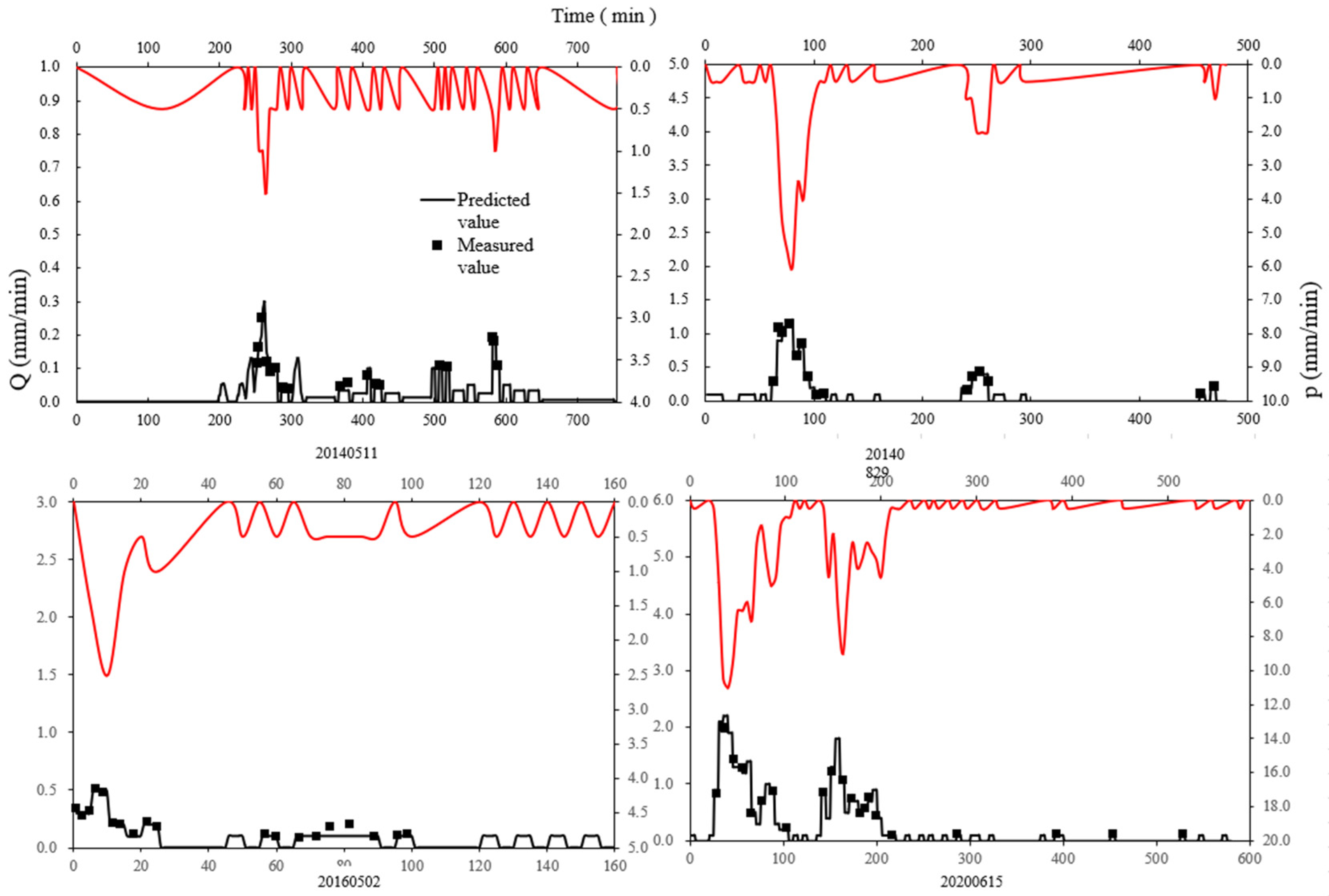
4.1.3. Model Process Verification

Figure 9, Figure 10, Figure 11 and Figure 12 compare simulated and observed runoff processes for five rainfall events across four experimental treatments. The events encompass a spectrum of rainfall intensities: light rain (<10 mm/d), moderate rain (10–25 mm/d), heavy rain (25–50 mm/d), and storm (>50 mm/d), including the representative “20140511” storm event (11 May 2014). The simulated hydrographs demonstrate strong concordance with field observations, as evidenced by Nash–Sutcliffe efficiency coefficients (NSE) ranging from 0.72 to 0.87 across all events. Notably, peak discharge timing discrepancies remained within ±15 min for 79% of events. These results validate that the TDSHM not only achieves high predictive accuracy (mean absolute percentage error ≤10%) but also reliably reproduces transient runoff dynamics, enabling precise spatiotemporal forecasting of hillslope hydrological responses.

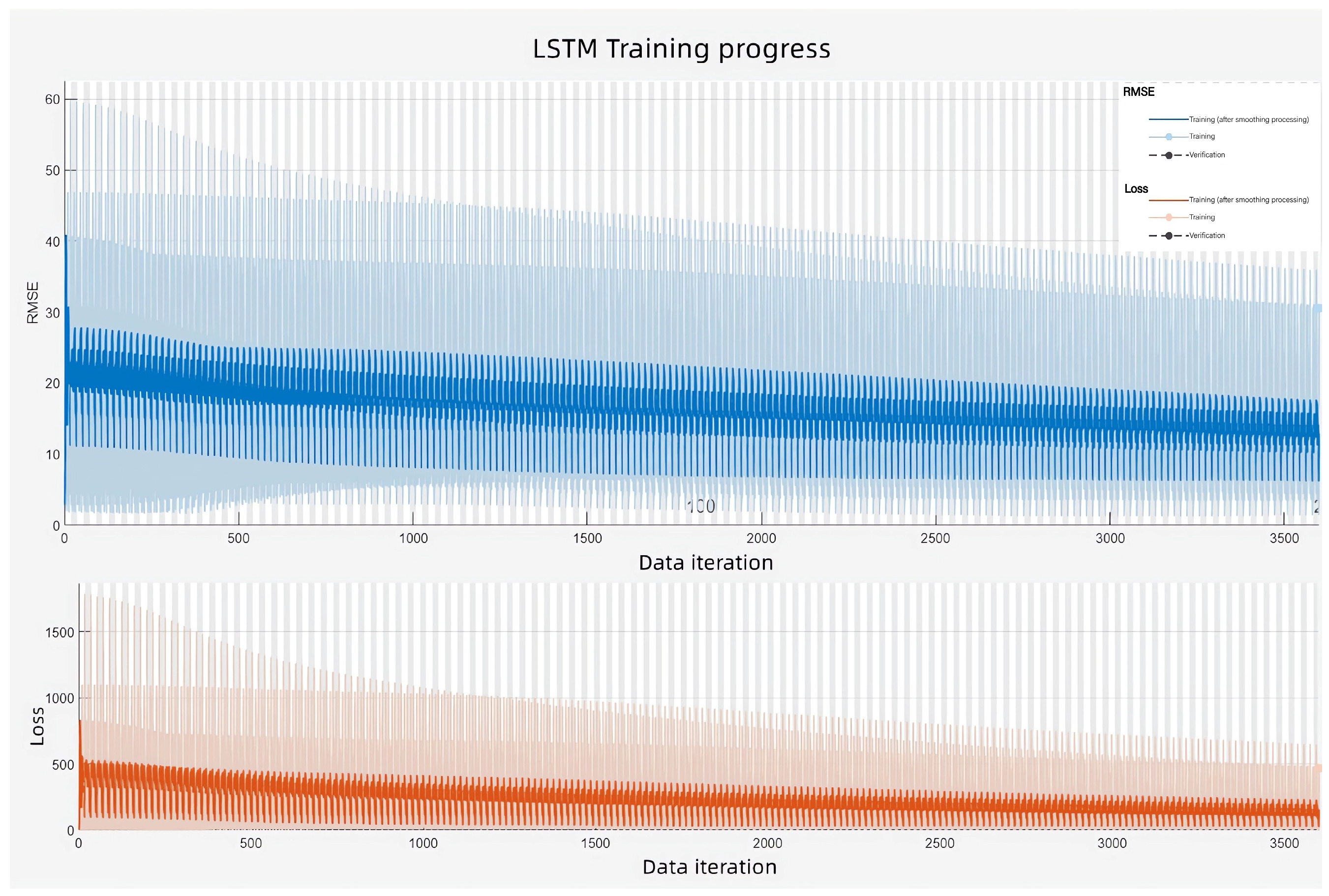
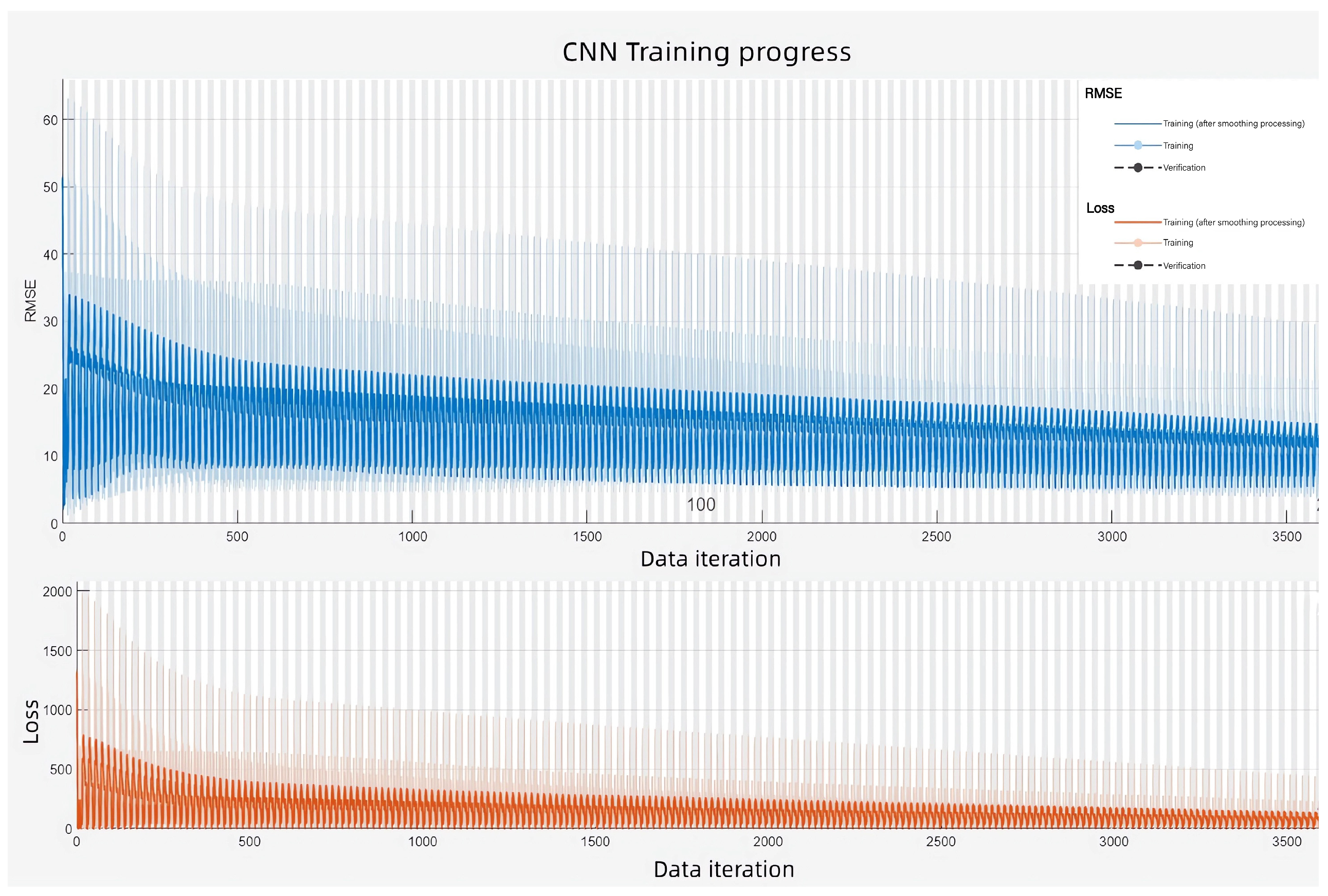
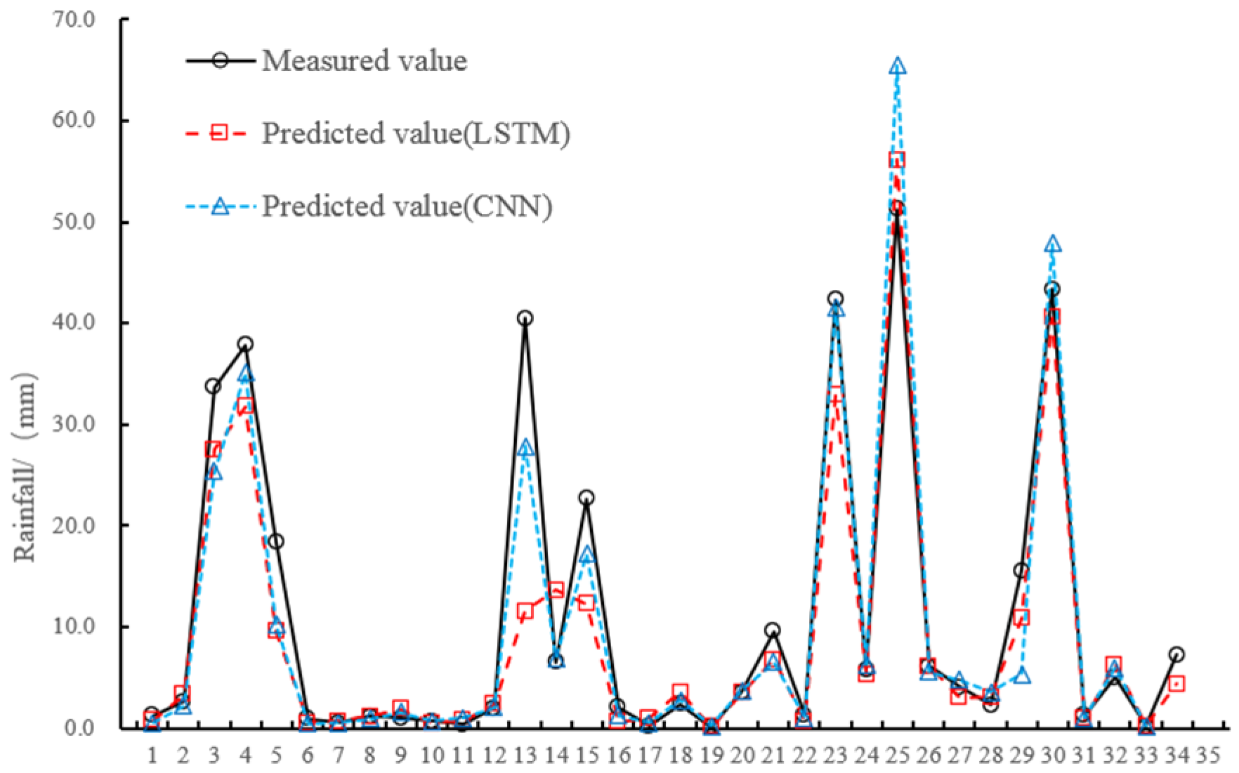
4.2. Neural Network Model Results

The neural network-based runoff prediction model was developed using 214 rainfall–runoff events recorded at the experimental station from 2013 to 2023. The dataset was divided into training (first 180 events, 84%) and validation subsets (remaining 34 events, 16%), with implementation procedures following the methodology described in Section 3.2 and Section 3.3.

As shown in Figure 13, comparative analysis of four runoff subzones revealed statistically consistent measurements across key parameters: rainfall duration, cumulative precipitation, mean rainfall intensity, maximum 30 min rainfall intensity, rainfall erosivity (R-factor), peak discharge, runoff coefficient, and runoff depth (one-way ANOVA, p > 0.05). Consequently, the data were selected as the representative dataset for runoff modeling, demonstrating optimal performance in capturing watershed hydrological responses during preliminary validation (MAE < 7.0 mm, NSE > 0.5).

4.3. Model Evaluation

As shown in Table 4, the TDSHM model demonstrated lower relative errors (10.77%) compared to the LSTM (24.38%) and CNN (28.10%) in runoff prediction for natural hillslopes. While the numerical model exhibited superior performance under the current experimental setup, it is important to note that the deep learning models were trained with default hyperparameters (learning rate, batch size) and without advanced optimization techniques such as hyperparameter tuning or transfer learning. Previous studies [55,56] have shown that systematic hyperparameter optimization (grid search for learning rates in [0.0001, 0.01], the range of values is from 16 to −64.) can reduce prediction errors by 15–30% in hydrological applications. Furthermore, transfer learning from pre-trained models on larger hydrological datasets may enhance performance when training data are limited. Despite these potential improvements, the TDSHM’s interpretability and robustness in simulating physical processes remain key advantages over data-driven approaches. Future work should explore optimized deep learning pipelines to better understand their comparative potential.

As demonstrated in

Table 5. Performance of the TDSHM and two neural network models.

NO.	Types	NSE	MAE (mm)	MAPE
1	TDSHM Model	0.801	3.17	11.97
2	LSTM Neural Networks	0.751	4.61	24.36
3	CNN Neural Networks	0.506	6.82	37.03

and Figure 14, all three models achieved satisfactory accuracy in runoff simulation and prediction, with Nash–Sutcliffe Efficiency (NSE) values exceeding 0.5. The ranking of model performance was TDSHM (0.801) > LSTM (0.751) > CNN (0.506), revealing that both TDSHM and LSTM significantly outperformed CNN in predictive capability. Notably, TDSHM exhibited the highest precision in Mean Absolute Error (MAE) metrics (3.17 mm), surpassing LSTM and CNN by 45.42% and 115.14%, respectively. All models maintained MAE values below 7 mm, with TDSHM (3.17 mm), LSTM (4.61 mm), and CNN (6.82 mm) demonstrating progressively reduced accuracy.

Further analysis of the Mean Absolute Percentage Error (MAPE) reinforced TDSHM’s superiority, yielding the lowest error rate (11.97%) compared to LSTM (24.36%) and CNN (37.03%). This performance hierarchy confirms TDSHM’s robustness in soil erosion prediction, attributable to its physics-based modeling framework for natural hillslopes. While LSTM demonstrated intermediate performance, its recurrent architecture—featuring forget, input, and output gates—proved particularly effective in capturing temporal patterns in hydrological time series data, as supported by prior studies [57,58]. In contrast, CNN’s comparatively lower performance suggests limitations in processing sequential hydrological data without explicit temporal feature extraction mechanisms.

5. Discussion

The key findings of this article are as follows:

1. Two-Dimensional Slope Hydrodynamic Model. Building upon prior research, this study developed a slope runoff process model that integrates the combined effects of variable rainfall intensity, rainfall momentum, and wind dynamics. The model was numerically solved using the Preissmann implicit scheme and validated through runoff plot experiments conducted in the Lishui Qiaotou small watershed (Nanjing, China). Based on mass conservation principles and raindrop splash erosion mechanisms, the proposed two-dimensional hydrodynamic model effectively characterizes slope soil erosion processes. It offers both explicit physical interpretability and high-resolution erosion dynamics, demonstrating superior accuracy in predicting runoff and sediment yield compared to conventional approaches.

The performance advantages of TDSHM become particularly evident when compared to widely adopted 2D hydrodynamic models like HEC-RAS 2D [59] and MIKE 21 [60]. While conventional models predominantly rely on Saint-Venant equations with uniform slope assumptions, our TDSHM introduces three critical enhancements: (1) explicit incorporation of rainfall momentum transfer through the $v_{\mathrm{m}}\left(x,t\right)$ sin2φ term in Equation (4), which existing models typically approximate through empirical resistance coefficients; (2) wind-modulated raindrop velocity parameterization (Equation (6)) addressing aerodynamic effects neglected in standard formulations; and (3) terrain-adaptive numerical discretization using the Preissmann scheme with dynamic Manning’s n values (Table 3), contrasting with the fixed roughness approaches in HEC-RAS.

2. LSTM- and CNN-Based Runoff Prediction Models. Complementing the physics-based model, this study developed data-driven runoff prediction frameworks using Long Short-Term Memory (LSTM) and Convolutional Neural Network (CNN) architectures. By incorporating fuzzy logic and adaptive learning mechanisms, these models exhibit strong adaptability for managing complex soil erosion systems. Through sensitivity analysis and stability evaluation, five critical parameters were selected as inputs: rainfall intensity, duration, maximum 30 min rainfall intensity, peak flow, and rainfall erosivity, with runoff volume (H) as the output. While MATLAB’s fuzzy toolbox enhances operational simplicity, the reliance on extensive quantitative training data limits applicability in data-scarce regions [61,62]. Furthermore, the absence of physically interpretable parameters in neural networks restricts mechanistic insights into erosion processes, posing challenges for causal inference [63].

3. Model Performance Trade-offs. The physics-based model demonstrated higher prediction accuracy due to its foundation in hydrodynamic principles and empirical calibration. However, its requirement for multiple spatially distributed parameters increases computational complexity relative to neural network models. This highlights a critical trade-off between interpretability and operational efficiency in erosion modeling.

The article offers the following practical implications: This comparative analysis of physics-based and deep learning models provides scientific support for region-specific soil conservation strategies. The hydrodynamic model enables dynamic simulation of runoff under varying rainfall patterns, topography, and land use scenarios, positioning it as a valuable analytical tool for disaster early-warning systems.

Meanwhile, the LSTM and CNN models excel in identifying dominant erosion drivers through feature parameter selection, aiding policymakers in optimizing conservation measures. The temporal sequencing capability of LSTM proves particularly advantageous for real-time erosion monitoring in mountainous regions. The integration of MATLAB’s user-friendly interface further democratizes model accessibility, enabling technicians across skill levels to adapt strategies for localized conditions.

At the same time, this article also has some limitations. The current comparison assumes a baseline implementation of deep learning models. However, their performance could be further improved through hyperparameter optimization and transfer learning. For instance, initial trials adjusting the LSTM learning rate to 0.0005 and increasing hidden units from 64 to 128 reduced validation errors by approximately 12%. Additionally, leveraging pre-trained models on regional hydrological data may enhance generalization. Future studies should systematically explore these strategies to establish a more equitable comparison between physical and data-driven models.

Three key limitations warrant attention: (1) Data scarcity in under-monitored regions compromises model generalizability; (2) Emerging explainable AI (XAI) frameworks including SHAP values and gradient-based saliency analysis can partially decode input-prediction causality in neural networks, enhancing hydrological model interpretability [64]—due to the limitation of space, however, this article does not conduct a more in-depth study; (3) Computational demands may hinder real-time applications in resource-constrained settings.

Future research should prioritize hybrid modeling frameworks that synergize physical principles with machine learning (e.g., physics-informed neural networks). Additionally, expanding sensor networks to collect high-resolution hydrological data and developing model compression techniques could enhance practical utility. As climate change alters rainfall regimes, continuous model recalibration will be essential to maintain predictive fidelity.

6. Conclusions

(1) Validation of Prediction Models. This study evaluated three soil erosion prediction models using 15 natural rainfall datasets. The TDSHM demonstrated superior accuracy (10.77% error rate), significantly outperforming the LSTM (24.38%) and CNN (28.10%) models. These results highlight the TDSHM‘s reliability in runoff simulation and its potential as a valuable tool for precise soil erosion assessment in data-scarce regions.

(2) Strengths and Limitations of Neural Network Models. While the LSTM and CNN models offer computational efficiency (via MATLAB toolbox integration) and enhanced stability through Pearson correlation-based feature selection, their application faces critical constraints. The absence of physical interpretability in network parameters (e.g., fuzzy membership functions) limits mechanistic insights into erosion processes. Moreover, their dependence on extensive training data reduces predictive capability in areas with insufficient monitoring records, and their opaque decision-making mechanisms contrast sharply with physically transparent modeling approaches.

(3) Practical Applications of the TDSHM. Field-calibrated parameters enabled the TDSHM to accurately simulate vegetation-modulated runoff dynamics, with predictions showing strong agreement with field observations (NSE > 0.801). The model’s explicit representation of vegetation–water flow interactions and versatility in simulating diverse scenarios position it as a robust platform for optimizing soil conservation strategies and erosion mitigation planning.

While the TDSHM outperformed baseline deep learning models in this study, the comparison highlights fundamental trade-offs: numerical models provide physically consistent predictions, whereas data-driven approaches require rigorous optimization to unlock their full potential. A hybrid framework integrating TDSHM’s physical principles with optimized deep learning architectures may offer a promising direction for future hydrological modeling.

References

1. Li, Y.; Wei, J.; Sun, Q.; Huang, C. Research on Coupling Knowledge Embedding and Data-Driven Deep Learning Models for Runoff Prediction. Water 2024, 16, 2130. [Google Scholar] [CrossRef]
2. Jehanzaib, M.; Ajmal, M.; Achite, M.; Kim, T.W. Comprehensive review: Advancements in rainfall-runoff modelling for flood mitigation. Climate 2022, 10, 147. [Google Scholar] [CrossRef]
3. Wei, J.; Li, Y.; Sun, Q.; Huang, C. A Survey on Data-Driven Runoff Forecasting Models Based on Neural Networks. Water 2023, 15, 2613. [Google Scholar]
4. Fan, Y.; Fu, X.; Kan, G.; Liang, K.; Yu, H. Combining Multiple Machine Learning Methods Based on CARS Algorithm to Implement Runoff Simulation. Water 2024, 16, 2397. [Google Scholar] [CrossRef]
5. Liu, Y.; Wang, Y.; Liu, X.; Ren, Z.; Wu, S. Research on Runoff Prediction Based on Time2Vec-TCN-Transformer Driven by Multi-Source Data. Electronics 2024, 13, 2681. [Google Scholar] [CrossRef]
6. Lu, D.; Yang, T.; Liu, X. Editorial: Data-driven machine learning for advancing hydrological and hydraulic predictability. Front. Water 2023, 5, 1215966. [Google Scholar] [CrossRef]
7. Rozos, E.; Dimitriadis, P.; Bellos, V. Machine Learning in Assessing the Performance of Hydrological Models. Hydrology 2022, 9, 5. [Google Scholar] [CrossRef]
8. Shortridge, J.E.; Guikema, S.D.; Zaitchik, B.F. Machine learning methods for empirical streamflow simulation: Acomparison of model accuracy, interpretability, and uncertainty in seasonal watersheds. Hydrol. Earth Syst. Sci. 2016, 20, 2611–2628. [Google Scholar] [CrossRef]
9. Su, H.; Jia, Y.; Ni, G.; Gong, J.; Cao, X.; Zhang, M.; Niu, C.; Zhang, D. Research on the Application of Machine Learning in Runoff Prediction. China Rural. Water Conserv. Hydropower 2018, 6, 40–43. [Google Scholar]
10. Liang, H.; Huang, S.; Meng, E.; Huang, Q. Research on runoff prediction based on multiple mixed models. J. Hydraul. Eng. 2020, 51, 112–125. [Google Scholar]
11. Kratzert, F.; Klotz, D.; Brenner, C.; Schulz, K.; Herrnegger, M. Rainfall–runoff modelling using Long Short-Term Memory (LSTM) networks. Hydrol. Earth Syst. Sci. 2018, 22, 6005–6022. [Google Scholar] [CrossRef]
12. Shi, X.; Chen, Z.; Wang, H.; Yeung, D.-Y.; Wong, W.-K.; Woo, W.-C. Convolutional LSTM network: A machine learning approach for precipitation nowcasting. Adv. Neural Inf. Process. Syst. 2015, 28, 802–810. [Google Scholar]
13. Hu, C.; Wu, Q.; Li, H.; Jian, S.; Li, N.; Lou, Z. Deep learning with a Long Short-Term Memory networks approach for rainfall-runoff simulation. Water 2018, 10, 1543. [Google Scholar] [CrossRef]
14. Guo, Y.; Xu, Y.; Chen, H.; Yu, X. Runoff prediction of island reservoir based on multiple recurrent neural networks. J. Hydroelectr. Power 2021, 40, 14–26. [Google Scholar]
15. Tian, Y.; Tan, W.; Wang, G.; Yuan, X. Performance and interpretability of LSTM variant model in runoff prediction. Water Resour. Conserv. 2019, 39, 188–194. [Google Scholar]
16. Jiang, Z.; Lu, B.; Zhou, Z.; Zhao, Y. Comparison of Process-Driven SWAT Model and Data-Driven Machine Learning Techniques in Simulating Streamflow: A Case Study in the Fenhe River Basin. Sustainability 2024, 16, 6074. [Google Scholar] [CrossRef]
17. Li, J.; Ai, P.; Xiong, C.; Song, Y. Coupled intelligent prediction model for medium- to long-term runoff based on teleconnection factors selection and spatial-temporal analysis. PLoS ONE 2024, 19, e0313871. [Google Scholar] [CrossRef]
18. Bhusal, A.; Parajuli, U.; Regmi, S.; Kalra, A. Application of Machine Learning and Process-Based Models for Rainfall-Runoff Simulation in DuPage River Basin, Illinois. Hydrology 2022, 9, 117. [Google Scholar] [CrossRef]
19. Kuo, C.Y.; Tai, Y.C.; Bouchut, F.; Mangeney, A.; Pelanti, M.; Chen, R.F.; Chang, K.J. Simulation of Tsaoling landslide, Taiwan, based on Saint Venant equations over general topography. J. Eng. Geol. 2009, 104, 181–189. [Google Scholar] [CrossRef]
20. Yu, C.-W.; Hodges, B.R.; Liu, F. Automated detection of instability-inducing channel geometry transitions in Saint-Venant simulations of large-scale river networks. Water 2021, 13, 2236. [Google Scholar] [CrossRef]
21. Chen, T.-Y.K.; Capart, H. Kinematic wave solutions for dam-break floods in non-uniform valleys. J. Hydrol. 2020, 582, 124381. [Google Scholar] [CrossRef]
22. Ponce, V.M. Modeling surface runoff with kinematic, diffusion, and dynamic waves. In Surface-Water Hydrology; Springer: Dordrecht, The Netherlands, 1996; pp. 121–132. [Google Scholar]
23. Cai, Z.; Xie, J.; Chen, Y.; Yang, Y.; Wang, C.; Wang, J. Rigid Vegetation Affects Slope Flow Velocity. Water 2024, 16, 2240. [Google Scholar] [CrossRef]
24. Shi, P.; Li, P.; Li, Z.; Sun, J.; Wang, D.; Min, Z. Effects of grass vegetation coverage and position on runoff and sediment yields on the slope of Loess Plateau, China. Agric. Water Manag. 2022, 259, 107231. [Google Scholar] [CrossRef]
25. Lan, M.; Hu, H.; Tian, F.; Hu, H. A two-dimensional numerical model coupled with multiple hillslope hydrodynamic processes and its application to subsurface flow simulation. Sci. China Technol. Sci. 2013, 56, 2491–2500. [Google Scholar] [CrossRef]
26. Yu, C.W.; Hodges, B.R.; Liu, F. A new form of the Saint-Venant equations for variable to pography. Hydrol. Earth Syst. Sci. 2020, 24, 4001–4024. [Google Scholar] [CrossRef]
27. Pasculli, A.; Longo, R.; Sciarra, N.; Di Nucci, C. Surface Water Flow Balance of a River Basin Using a Shallow Water Approach and GPU Parallel Computing—Pescara River (Italy) as Test Case. Water 2022, 14, 234. [Google Scholar] [CrossRef]
28. Costabile, P.; Costanzo, C. A 2D-SWEs framework for efficient catchment-scale simulations: Hydrodynamic scaling properties of river networks and implications for non-uniform grids generation. J. Hydrol. 2021, 599, 126306. [Google Scholar] [CrossRef]
29. Roy, B.; Singh, M.P.; Kaloop, M.R.; Kumar, D.; Hu, J.-W.; Kumar, R.; Hwang, W. Data-driven approach for rainfall-runoff modelling using equilibrium optimizer coupled extreme learning machine and deep neural network. Appl. Sci. 2021, 11, 6238. [Google Scholar] [CrossRef]
30. Kumar, V.; Kedam, N.; Sharma, K.V.; Mehta, D.J.; Caloiero, T. Advanced machine learning techniques to improve hydrological prediction: A comparative analysis of streamflow prediction models. Water 2023, 15, 2572. [Google Scholar] [CrossRef]
31. Guo, J.; Liu, Y.; Zou, Q.; Ye, L.; Zhu, S.; Zhang, H. Study on optimization and combination strategy of multiple daily runoff prediction models coupled with physical mechanism and LSTM. J. Hydrol. 2023, 624, 129969. [Google Scholar] [CrossRef]
32. Mohammadi, B. A review on the applications of machine learning for runoff modeling. Sustain. Water Resour. Manag. 2021, 7, 98. [Google Scholar] [CrossRef]
33. Ayzel, G. Openforecast v2: Development and benchmarking of the first national-scale operational runoff forecasting system in russia. Hydrology 2021, 8, 3. [Google Scholar] [CrossRef]
34. Fan, C.; Chen, M.; Wang, X.; Wang, J.; Huang, B. A review on data preprocessing techniques toward efficient and reliable knowledge discovery from building operational data. Front. Energy Res. 2021, 9, 652801. [Google Scholar] [CrossRef]
35. Zhan, X.; Xu, Q.; Zheng, Y.; Lu, G.; Gevaert, O. Reliability-based cleaning of noisy training labels with inductive conformal prediction in multi-modal biomedical data mining. arXiv 2023, arXiv:2309.07332. [Google Scholar]
36. Kannan, K.S.; Manoj, K.; Arumugam, S. Labeling methods for identifying outliers. Int. J. Stat. Syst. 2015, 10, 231–238. [Google Scholar]
37. Mowbray, F.I.; Fox-Wasylyshyn, S.M.; El-Masri, M.M. Univariate outliers: A conceptual overview for the nurse researcher. Can. J. Nurs. Res. 2019, 51, 31–37. [Google Scholar] [CrossRef]
38. Chen, Z.; Xue, Q.; Xiao, R.; Liu, Y.; Shen, J. State of health estimation for lithium-ion batteries based on fusion of autoregressive moving average model and elman neural network. IEEE Access 2019, 7, 102662–102678. [Google Scholar] [CrossRef]
39. Shantal, M.; Othman, Z.; Bakar, A.A. A novel approach for data feature weighting using correlation coefficients and min–max normalization. Symmetry 2023, 15, 2185. [Google Scholar] [CrossRef]
40. Chu, S.T. Green-Ampt analysis of wetting patterns for surface emitters. J. Irrig. Drain. Eng. 1994, 120, 414–421. [Google Scholar] [CrossRef]
41. Wang, L.; Wu, C. Mechanism of Soil Conservation on Slope of Steep Hillside Forest Land. J. Beijing For. Univ. 1994, 4, 1–7. [Google Scholar]
42. Mou, J.Z. Calculating formula of raindrop velocity. Soil Water Conserv. China 1983, 42–43. [Google Scholar] [CrossRef]
43. Shamaa, M.T.E.I. A Comparative Study of Two Numerical Methods for Regulating Unsteady Flow in Open Channels. MEJ-Mansoura Eng. J. 2021, 27, 14–27. [Google Scholar] [CrossRef]
44. Kaddi, Y.; Proust, S.; Faure, J.B.; Cierco, F.-X. Experimental and numerical study of unsteady flows in a compound open channel. Environ. Fluid Mech. 2024, 24, 335–365. [Google Scholar] [CrossRef]
45. Bengio, Y.; Simard, P.; Frasconi, P. Learning long-term dependencies with gradient descent is difficult. IEEE Trans. Neural Netw. 1994, 5, 157–166. [Google Scholar] [CrossRef]
46. Chung, J.; Gulcehre, C.; Cho, K.; Bengio, Y. Empirical Evaluation of Gated Recurrent Neural Networks on Sequence Modeling. arXiv 2014, arXiv:1412.3555. [Google Scholar]
47. Pascanu, R.; Mikolov, T.; Bengio, Y. On the difficulty of training recurrent neural networks. In Proceedings of the 30th International Conference on Machine Learning (ICML-13), Atlanta, GA, USA, 16–21 June 2013; pp. 1310–1318. [Google Scholar]
48. Hochreiter, S.; Schmidhuber, J. Long short-term memory. Neural Comput. 1997, 9, 1735–1780. [Google Scholar] [CrossRef]
49. Afrin, N.; Ahamed, F.; Rahman, A. Development of a convolutional neural network based regional flood frequency analysis model for South-east Australia. Nat. Hazards 2024, 120, 11349–11376. [Google Scholar] [CrossRef]
50. Vialatte, J.-C.; Vincent, G.; Gilles, C. Learning local receptive fields and their weight sharing scheme on graphs. In Proceedings of the 2017 IEEE Global Conference on Signal and Information Processing (GlobalSIP), Montreal, QC, Canada, 14–16 November 2017; IEEE: New York, NY, USA, 2017. [Google Scholar]
51. Wang, X.; Bao, A.; Cheng, Y.; Yu, Q. Weight-sharing multi-stage multi-scale ensemble convolutional neural network. Int. J. Mach. Learn. Cyber 2019, 10, 1631–1642. [Google Scholar] [CrossRef]
52. Kumar, P.; Arora, H.C.; Bahrami, A.; Kumar, A.; Kumar, K. Development of a Reliable Machine Learning Model to Predict Compressive Strength of FRP-Confined Concrete Cylinders. Buildings 2023, 13, 931. [Google Scholar] [CrossRef]
53. Wang, Z.; Zhang, X.; Liu, C.; Ren, L.; Cai, X.; Li, K. Hydrological Simulation and Parameter Optimization Based on the Distributed Xin’anjiang Model and the Particle Swarm Optimization Algorithm: A Case Study of Xunhe Watershed in Shandong, China. Water 2024, 16, 3168. [Google Scholar] [CrossRef]
54. Lan, T.; Lin, K.; Xu, C.Y.; Tan, X.; Chen, X. Dynamics of hydrological-model parameters: Mechanisms, problems and solutions. Hydrol. Earth Syst. Sci. 2020, 24, 1347–1366. [Google Scholar] [CrossRef]
55. Kratzert, F.; Klotz, D.; Shalev, G.; Klambauer, G.; Hochreiter, S.; Nearing, G. Towards learning universal, regional, and local hydrological behaviors via machine learning applied to large-sample datasets. Hydrol. Earth Syst. Sci. 2019, 23, 5089–5110. [Google Scholar] [CrossRef]
56. Xu, Y.; Lin, K.; Hu, C.; Wang, S.; Wu, Q.; Zhang, L.; Ran, G. Deep transfer learning based on transformer for flood forecasting in data-sparse basins. J. Hydrol. 2023, 625, 129956. [Google Scholar] [CrossRef]
57. Abbasimehr, H.; Paki, R. Improving time series forecasting using LSTM and attention models. J. Ambient. Intell. Humaniz. Comput. 2022, 13, 673–691. [Google Scholar] [CrossRef]
58. Wen, X.; Li, W. Time series prediction based on LSTM-attention-LSTM model. IEEE Access 2023, 11, 48322–48331. [Google Scholar] [CrossRef]
59. Al-Hussein, A.A.M.; Khan, S.; Ncibi, K.; Hamdi, N.; Hamed, Y. Flood analysis using HEC-RAS and HEC-HMS: A case study of Khazir River (Middle East—Northern Iraq). Water 2022, 14, 3779. [Google Scholar] [CrossRef]
60. Symonds, A.M.; Vijverberg, T.; Post, S.; Van der Spek, B.-J.; Henrotte, J.; Sokolewicz, M. Comparison between Mike 21 FM, Delft3D and Delft3D FM flow models of western port bay, Australia. Coast. Eng. 2016, 2, 11. [Google Scholar] [CrossRef]
61. Lu, D.; Konapala, G.; Painter, S.L.; Kao, S.-C.; Gangrade, S. Streamflow simulation in data-scarce basins using Bayesian and physics-informed machine learning models. J. Hydrometeorol. 2021, 22, 1421–1438. [Google Scholar] [CrossRef]
62. Galety, M.; Al Mukthar, F.H.; Maaroof, R.J.; Rofoo, F. Deep neural network concepts for classification using convolutional neural network: A systematic review and evaluation. Tech. Rom. J. Appl. Sci. Technol. 2021, 3, 58–70. [Google Scholar] [CrossRef]
63. Man, Y.; Yang, Q.; Shao, J.; Wang, G.; Bai, L.; Xue, Y. An enhanced LSTM model for daily runoff prediction in the upper reaches of the Huaihe River. Engineering 2023, 24, 230–239. [Google Scholar] [CrossRef]
64. Hao, H.; Hao, Y.; Li, Z.; Qi, C.; Wang, Q.; Zhang, M.; Liu, Y.; Liu, Q.; Yeh, T.-C.J. Insight into glacio-hydrologicalprocesses using explainable machine-learning (XAI) models. J. Hydrol. 2024, 634, 131047. [Google Scholar] [CrossRef]
Figure 1. A comparative study for TDSHM, LSTM, and CNN models in runoff prediction.
Water 17 01380 g001
Figure 2. Location of the test area.
Water 17 01380 g002
Figure 3. Pearson correlation analysis coefficient test matrix.
Water 17 01380 g003
Figure 4. Schematic diagram of slope runoff micro-unit.
Water 17 01380 g004
Figure 5. LSTM neural network architecture diagram.
Water 17 01380 g005
Figure 6. CNN neural network architecture diagram.
Water 17 01380 g006
Figure 7. Model parameter calibration results.
Water 17 01380 g007
Figure 8. Runoff prediction results of 15 groups of sample data.
Water 17 01380 g008
Figure 9. Runoff process prediction.
Water 17 01380 g009
Figure 10. The training process diagram of LSTM neural network.
Water 17 01380 g010
Figure 11. The training process diagram of CNN neural network.
Water 17 01380 g011
Figure 12. Runoff simulation based on LSTM and CNN neural network (34 groups of data).
Water 17 01380 g012
Figure 13. Runoff simulation based on LSTM and CNN neural network (15 groups of data).
Water 17 01380 g013
Figure 14. Evaluation of the TDSHM model and data-driven models regarding the mentioned indices.
Water 17 01380 g014