Evaluation of Micrometeorological Models for Estimating Crop Evapotranspiration Using a Smart Field Weighing Lysimeter

Abstract

Accurate estimation of crop water use, which is expressed as evapotranspiration (ET) is an important task for effective irrigation and agricultural water management. Although direct field measurement of actual evapotranspiration (ETa) is the most reliable method, practical and economic limitations often make it difficult to acquire, especially in developing countries. Consequently, crop evapotranspiration (ETc) is calculated using reference evapotranspiration (ETo) and crop-specific coefficients (Kc) to support irrigation water management practices. Several ETo models have been developed to address varying environmental conditions; however, their transferability to new environments often leads to under or over estimation of ETo, which has an impact on ETc estimation. This study evaluated the accuracy of 30 ETo micrometeorological models to estimate ETc under different seasonal and micro-climatic conditions using ETa data directly measured using a smart field weighing lysimeter as a benchmark. Local Kc values were derived from field-based measurements, while statistical metrics were applied for the evaluation process. A cumulative ranking approach was used to assess the accuracy and consistency of the models across four cropping seasons. Results demonstrated the Penman–Monteith model to be the most consistent model in estimating ETc, which outperformed other models across all cropping seasons. The performance of alternative models differed significantly with seasonal conditions, indicating their susceptibility to seasonality. The findings demonstrated the Penman–Monteith model as the most reliable approach for estimating ETc, which justifies its application role as a benchmark for validating other ETo models in data-limited areas. The study emphasizes the importance of site-specific validation and calibration of ETo models to improve their accuracy, applicability, and reliability in diverse environmental conditions.

1. Introduction

Reference evapotranspiration (ETo) is a crucial component of irrigated agriculture and represents the rate at which water is transferred from cropped land and plant surfaces to the atmosphere under specific climatic conditions [1]. This component serves as a benchmark for determining crop water needs for several crops, thereby assisting in the efficient management of irrigation practices [2]. In arid regions, water resources are scarce and evaporative demands are high, which makes agricultural production face acute challenges with limited water supplies [3]. Arid regions suffer more water scarcity; as a result, declines in precipitation amounts have led to the supplementation of crops with irrigation water from different water surfaces and groundwater sources [4]. A critical challenge is how this precious resource can be conserved effectively. What happens to the water after each irrigation event can be the answer to this question concern. To maintain water use efficiency, accurate quantification of evapotranspiration (ET) is required to determine a precise supply of water as required by crops and not based on the irrigator or farmer perceptions. To maintain a balance, accurate determination of ET is critical. Therefore, the significance of ETo cannot be overstated; this component plays a critical role in simulating crop evapotranspiration (ETc) when ET cannot be measured directly. High accuracy when determining this component is important; this component directly influences irrigation scheduling, water resource planning, and the sustainability of agricultural systems [5].

Efficient water use conserves available water resources while also mitigating the adverse effects of over-irrigation such as increased soil salinization, degradation, and groundwater depletion [6]. In the process of determining irrigation water requirements for a specific crop when there are no direct measuring devices, ETo is multiplied by a crop coefficient (Kc) value of a specific crop to be irrigated during its current growth stage to determine ETa; the latter is equivalent to the actual evapotranspiration (ETa). In this process, Allen et al. [1] described the term ETo as resembling atmospheric water or evaporative demand, whereas the Kc values resemble a broader integration of crop-based factors that distinguishes the crop from other crops or the reference grass based on the energy balance. The Kc values for many crops that are grown globally to feed nations have been determined and published by the Food and Agriculture Organization (FAO) on their drainage and irrigation [1]. This was done over two and a half decades ago using crops that were suitable for climatic and environmental conditions. However, climate variability and changes in rainfall patterns with South Africa’s rainfall being erratic in most regions has been reported [7]. With such natural changes and intensified aridity in many regions, agricultural practitioners and stakeholders have resorted to the use of crop cultivars that are drought tolerant [8]. The assumption is that their crop water requirements may vary compared with those of the cultivars used in determining Kc values in recent decades. Although ETo and Kc values are essential for calculating ETc, emerging approaches on remote sensing are under development that offer alternative methods for estimating ETc relying on energy balance approaches other than those which rely solely on these parameters. However, local calibration and adjustments of some parameters remain crucial for model improvements and validation; in this case, direct measurements are required to determine ETa using approaches such as the water balance. The challenging part of this task is the lack of measurement devices, which are expensive and not economically practical to install for every parcel of land, especially in developing countries where cash flow is in tight budgets and prioritized projects. Measured ETa is the biggest data gap in South Africa, and models are normally benchmarked using standardized methods rather than real-time data reflecting the true field conditions [9]. However, they are still critical, particularly for calibration purposes and the determination of Kc values. Although scientists still rely on published Kc values, their adjustment to local conditions is crucial. A review by Pereira et al. [10] highlighted several challenges associated with the transferability of Kc values. In their review, they also reported that Kc values have been used in many studies and have been updated at local scales where ETa was measured using accurate devices such as lysimeters.

The lack of ETa in situ data dates back to two centuries when Dalton [11] developed an empirical model to estimate ETo. Since Dalton [11], several models have been developed, including those by Meyer [12], Thornthwaite [13], Penman [14], and Trajkovic [15]. ETo models simulate ETo based on climatic variables such as temperature, humidity, wind speed, and solar radiation. As a result, these variables have led to the classification of ETo models into four classes: radiation models, temperature models, aerodynamic-based models, and combination models [16]. DehghaniSanij et al. [17] reported that most of these models were developed, validated, and calibrated in temperate regions. The fact that they were developed in temperate environments makes them require rigorous validation and calibration to ensure their accuracy and reliability when transferred and applied in different environments from those of their origin [18]. The validation process involves comparing model outputs with observed data to assess their performance, while the calibration process fine-tunes model parameters to local conditions. These steps are critical because even minor inaccuracies in ETo estimates can lead to significant errors in irrigation planning, potentially resulting in either water shortages or excessive usage.

Several studies have evaluated the performance of different micrometeorological models in different regions specifically for the determination of ETo, and their results demonstrated that different models are usually accurate when applied to the climate conditions under which they were developed and calibrated [19,20,21]. The limitation that arises from the use of models is their transferability from environments in which they were developed and calibrated into regions with different climatic and topographical settings, which vary spatially [22]. As a result, models that are adopted and applied outside their region of origin have high uncertainties, resulting in poor performance. For example, Moeletsi et al. [23] compared the performance of two temperature-based models, namely Hargreaves and Samani [24] and Thornthwaite [13], to estimate decadal ET in Free State South Africa against the Penman–Monteith model; their selection was based on “availability-for-use” data, wherein temperature is a common available variable measured by most weather stations in South Africa. They reported that, compared with the calibrated Thornwaite model, the uncalibrated models provided very poor results, underestimating ET, whereas the calibrated Hargreaves and Samani models yielded accurate accuracy ranges. The major emphasis of their work was that all models used were developed outside South Africa, and their applications require validation and calibration to local conditions.

The Penman–Monteith model of the FAO has frequently been proposed for estimating ETo, but its accuracy and reliability are hampered by its data requirements, which is particularly challenging in areas with limited data availability, such as some South African areas with limited weather stations [23]. The FAO developed and introduced the standard ETo model as a combination model to solve irrigation scheduling problems worldwide [1]. Although a standard model exists, its limitations cannot be undermined; the Penman–Monteith model was developed based on a reference crop fully watered and continuously growing at a constant height [1]. The assumption that crops have an ample supply of water is not true in arid environments with limited rainfall and water resources [25].

This study aimed at evaluating ETc estimation by testing 30 ETo micrometeorological models at the farm level across different cropping seasons. Unlike many previous studies in South Africa which primarily compared ETo estimates from different models with a standard model, this study focuses on the accuracy of ETc derived from ETo models using a smart field weighing lysimeter to directly measure ETa. This study assesses the models’ performance through statistical metrics to determine their suitability for estimating ETc at local micro-climatic conditions and seasons. This study aims to identify models that reliably estimate ETc across diverse seasonal conditions and cropping systems, which addresses the challenges of model transferability and data limitations. The use of real-time measurements with the high-accuracy lysimeter at the field scale makes the results of this study important for improving irrigation water management and sustainable agricultural practices, particularly in data-scarce environments. This direct measurement approach significantly reduces the uncertainties associated with model assumptions and enhances the calibration and validation of micrometeorological models. This study also aims to adjust Kc values to emphasize the role of local calibration when dealing with irrigation water management; any slight adjustments in Kc values might also mean a change in irrigation scheduling. The Kc value adjustments build upon published works such as the FAO-56, were Kc values which were developed in areas outside of South Africa using crop cultivars that were suitable then. However, with drought-tolerant cultivars, the crop water requirements are prone to change. Reliable ETo models can ensure accurate estimation of crop water requirements, minimizing over- or under-irrigation.

2. Materials and Methods

2.1. Study Area

This study was carried out on an 18 ha experimental farm owned by the South African Barley Breeding Institute (SABBI) near the town of Hartswater, which is an agricultural hub in the Frances Baard district municipality in the Northern Cape Province of South Africa (Figure 1). The farm is located at the central coordinates with latitude 24°44′25″ E and longitude −27°43′15″ S (Figure 1). The study area is within South Africa’s largest irrigation scheme, known as the Vaalharts irrigation scheme. This scheme was established in the early 1930s to alleviate unemployment and poverty [26]. The study area is in the country’s arid region with water limitations, receiving irrigation water through transfers, predominantly from the Vaal River through the Bloemhof dam and constructed open canals [27]. Most farms are irrigated with pivot irrigation systems, although flood irrigation, sprinklers, drip irrigation, and other methods continue to be employed [28]. Annually, between November and March, the area receives approximately 450 mm of rain on the Taung side and approximately 477 mm on the Jan Kempdorp side [29]. Temperatures in the area have been recorded as high as 48.8 °C and as low as −4.4 °C [29]. Ref. [30] defined the soils in the study area as sandy loam in texture. Salinity has been extensively researched in this area as a major issue that limits groundwater usage [29]. The area is well known for its pecan production; however, it also grows winter wheat, barley, maize, groundnuts, sorghum, cotton, lucerne, soybeans, tobacco, and other cash crops [31]. Limited cattle and poultry farming also exist [32]. This study area was chosen based on the availability of weather stations, a suitable arid environment with limited water, and the variety of crops used to assess crop water usage.

2.2. Meteorological and Lysimeter Data Acquisition

2.2.1. Acquisition of Meteorological Data

The meteorological data were obtained from an automatic weather station installed in the experimental field for four cropping seasons located at the following coordinates: 24° 44′ 29.43″ E and −27° 43′ 14.82″ S (Figure 2) at an elevation of 1092 m above sea level. The weather station measured and recorded various climate variables, which allowed for the computation of ETo while also serving as a tool to understand the local climate of the study area. The measured variables were measured at a 10 min temporal resolution, whereas some variables were measured on an hourly basis. A tipping bucket rain gauge linked to the weather station facilitated precise measurements of irrigation and natural precipitation, which is crucial for understanding irrigation amounts. To ensure the accuracy of meteorological data, all sensors at each weather station were calibrated at the beginning of each cropping season and periodically checked for consistency; this detail is well explained in the climate datasets of South Africa, of which the weather stations used are a part, as explained by Moeletsi et al. [34]. The calibration procedures followed manufacturer-recommended protocols, and detailed logs were maintained to document the calibration dates and outcomes. The sensors measured climate variables at 10 min intervals, ensuring high-resolution data. Routine maintenance and testing were conducted monthly to prevent drift in sensor accuracy, particularly for critical components such as the tipping bucket rain gauge and temperature sensors.

2.2.2. Actual Evapotranspiration Determination Using a Smart Field Weighing Lysimeter

To determine the ETa, smart field weighing lysimeters (SFL-600) developed by METER Group^©, Pullman, Washington, USA were installed and used to measure different components of the water balance from 2019 through to 2021, and more data are being collected through continuous projects (

Table 1. Measurements of ETa and cropping seasons for different crop types.

Cropping Season	Measurement Year	Crop Type
Season 1 winter	2019	Barley
Season 2 summer	2019–2020	Maize
Season 3 winter	2020	Barley
Season 4 summer	2020–2021	Soybean

). According to our knowledge, this is the first lysimeter of its kind in the country. Its introduction attempts to fill the gap of direct field ETa measurements in the country, which limits its extrapolation to non-agricultural zones outside its reference region. The installation process involved placing specialized lysimeter cylinders, each equipped with a weighing balance mechanism, into protective barrels occupying excavated holes in the ground. These protective barrels were sealed with impermeable rubber membranes to isolate the soil column within the lysimeters. To capture detailed data on the soil–water relationship, sensors were placed at multiple depths within each lysimeter (5, 30, and 55 cm). The sensors were designed to measure various essential parameters, including temperature, moisture content, water potential, and soil electrical conductivity. This allowed for a detailed characterization of the soil–water conditions and how they changed over time. The sensors were connected to a data logger system, which recorded data at minute intervals. This frequent data collection ensured a high-resolution dataset, providing insights into the dynamic soil–water interactions.

2.3. Methods Used for Determining ETo from Meteorological Data and ETa from Lysimeter Data

Model Selection for Estimation of ETo

A total of 30 micrometeorological models for estimating ETo were used to estimate ETc for the four cropping seasons. The selected models were chosen based on their historical use, relevance to arid and semi-arid agro-climatic conditions, and availability of input data that aligned with the study’s resources. Geographical representativeness was a key criterion, with models originating from diverse climatic backgrounds to ensure a robust evaluation. The choice was further motivated by the need for comprehensive evaluation across different classes of micrometeorological models, including radiation-based, temperature-based, aerodynamic, and combination models. This extensive range allows for a robust assessment of their performance under diverse climatic and seasonal conditions, ensuring that the findings provide a reliable basis for selecting the most suitable models for specific applications. While the volume may seem extensive, it was necessary to encompass the breadth of models developed over decades to address varying environmental challenges. Models beyond the selected 30 were excluded either due to limited applicability in the study’s arid and semi-arid context, lack of required input parameters, or insufficient documentation for accurate implementation and comparison. Radiation-based models, as shown in

Table 2. Radiation-based models for estimating ETo.

ETo Model	Equation	Input Parameters	References
ETo_P-T	${\displaystyle \frac{1}{\mathsf{\lambda }}}\left[\mathsf{\alpha }{\displaystyle \frac{\Delta }{\Delta +\mathsf{\gamma }}}\left({\mathrm{R}}_{\mathrm{n}}-\mathrm{G}\right)\right]$	Elevation; Tmean; SR	[21]
ET-Makkink	$0.7\left({\displaystyle \frac{\mathrm{Rs}}{\mathsf{\lambda }}}\right)\left[{\displaystyle \frac{\Delta }{\Delta }}+\mathsf{\gamma }\right]-0.12$	Elevation; Tmean; SR	[19]
Turc	$0.0133\times \left({\displaystyle \frac{\mathrm{Tm}}{\mathrm{Tm}+15}}\right)\times \left(\mathrm{Rs}+50\right)\mathrm{if}\mathrm{RH}>50\%$ $0.0133\times \left({\displaystyle \frac{\mathrm{Tm}}{\mathrm{Tm}+15}}\right)\times \left(\mathrm{Rs}+50\right)\times \left(1+50-{\displaystyle \frac{\mathrm{RH}}{70}}\right)\left(\mathrm{if}\mathrm{RH}<50\%\right)$	Tmean; SR; RHmean	[35]
Hansen	$0.408\times 0.70\left({\displaystyle \frac{\Delta }{\Delta +\mathsf{\gamma }}}\right)\mathrm{Rs}$	SR	[36]
Irmak_Rn	$-0.611+0.149\times \mathrm{Rs}+0.079\mathrm{Tmean}$	SR; Tmean	[37]
Irmak_Rs	$(3.75+0.503{\mathrm{u}}_2)\left(\mathrm{es}-\mathrm{ea}\right)$	SR; Tmean	[37]
Jensen-Haisen	$\mathrm{Rs}\left(0.025\times \mathrm{T}+0.08\right)$	Tmean; SR	[38]
Tabari 1	$-0.642+0.174\mathrm{Rs}+0.0353\mathrm{Tmean}$	Tmean; SR	[39]
Tabari 2	$-0.478+0.156\mathrm{Rs}-0.0112\mathrm{Tmax}+0.0733\mathrm{Tmin}$	SR; Tmax; Tmin.	[39]
Caprio	$\left(0.01092708\times \mathrm{T}\right)+\left(0.0060706\times \mathrm{Rs}\right)$	Tmean; SR	[40]
Calibrated Christiansen	$0.53\times ({\displaystyle \frac{\mathrm{Rs}}{\mathsf{\lambda }}})$	RS	[41]

, estimate ET using solar radiation (Rs), temperature (T), and humidity (RH). As solar radiation increases, the energy available for water evaporation increases, which increases ET from soil and plants [33]. The temperature drives this process by warming the land surface, which increases the vaporization rate. Relative humidity helps in modeling moisture potential, which defines how much water vapor can be drawn into the air [34]. In the temperature-based models shown in

Table 3. Temperature-based models for estimating ETo.

Reference Evapotranspiration Model	Equation	Input Parameters	References
Ivanov	$0.00006\times {\left(25+\mathrm{Tmean}\right)}^2\times \left(100-\mathrm{RH}\right)$	Mean Temperature; Mean Relative Humidity	[42]
Trajkovic	${\displaystyle \frac{\left[0.0023\mathrm{Ra}\left(\mathrm{Tmean}+17.8\right){\left(\mathrm{Tmax}-\mathrm{Tmin}\right)}^{0.424}\right]}{\mathsf{\lambda }}}$	Latitude; Tmean; Tmax; Tmin	[15]
Schendel	$16\times \left({\displaystyle \frac{\mathrm{Tmean}}{\mathrm{RH}}}\right)$	Tmean; RH	[43]
Ravazzani	$\left(0.817+0.00022\times \mathrm{Z}\right)0.0023\mathrm{Ra}\left(\mathrm{Tmean}+17.8\right){\left(\mathrm{T}\max -\mathrm{Tmin}\right)}^{0.5}$	Elevation; Tmean; Tmax; Tmin;	[44]
Hamon	$\mathrm{k}\left(0.1651\times 216.7\right)\mathrm{N}\times ({\displaystyle \frac{\mathrm{es}}{\mathrm{T}+272.3}})$	Tmean; Tmax; Sunshine Hours	[45]
Papadakis	$2.5\left(\mathrm{es}-\mathrm{ea}\right)$	Tmax; Tmin	[46]
Droogers and Allen	$0.003\times \left(\mathrm{Tmean}+20\right){\left(\mathrm{Tmax}-\mathrm{Tmin}\right)}^{0.4}\mathrm{Ra}$	Latitude; Tmean; Tmax; Tmin.	[47]
Hargreaves and Allen	$\left(0.0135\mathrm{Tmean}+0.2403\right)\times {\displaystyle \frac{\mathrm{Rs}}{\mathsf{\lambda }}}$	Tmean; SR	[20]
Hargreaves and Samani	${\displaystyle \frac{\left[0.0023\times \mathrm{Ra}\left(\mathrm{Tmean}+17.8\right){\left(\mathrm{Tmax}-\mathrm{Tmin}\right)}^{0.5}\right]}{\mathsf{\lambda }}}$	Latitude; Mean Temperature; Maximum Temperature; Minimum Temperature.	[24]

, temperature is the primary driver of ET. Higher temperatures provide more energy for water to evaporate, promoting ET. Some models also consider potential radiation (PR) as a supplementary factor. The aerodynamic-based models in

Table 4. Aerodynamic-based models for estimating ETo.

Reference Evapotranspiration Model	Equation	Input Parameters	References
ET_Albrecht	$\left(0.1005+0.297\times {\mathrm{u}}_2\right)\times \left(\mathrm{es}-\mathrm{ea}\right)$	Tmax; Tmin; RHmax; MeanU2; RHmin	[48]
Trabert	$0.408\times \left(0.3075\times \sqrt{{\mathrm{u}}_2}\right)\times \left(es-ea\right)$	Tmax; Tmin; RHmax; MeanU2; RHmin	[49]
Meyer	$\left(3.75+0.503{\mathrm{u}}_2\right)\left(\mathrm{es}-\mathrm{ea}\right)$	Tmax; Tmin; RHmax; MeanU2; RHmin.	[12]
WMO	$\left(1.298+0.934{\mathrm{u}}_2\right)\left(\mathrm{es}-\mathrm{ea}\right)$	Tmax; Tmin; RHmax; MeanU2; RHmin.	[50]
ROhWER	$\left(3.3+0.891{\mathrm{u}}_2\right)\left(\mathrm{es}-\mathrm{ea}\right)$	Tmax; Tmin; RHmax; MeanU2; RHmin	[51]
Brockamp–Wenner	$\left(0.543{{\mathrm{u}}_2}^{0.456}\right)\left(\mathrm{es}-\mathrm{ea}\right)$	Tmax; Tmin; RHmax; MeanU2; RHmin	[52]
Penman	$0.35\times \left(1+0.24\times {\mathrm{u}}_2\right)\times \left(\mathrm{es}-\mathrm{ea}\right)$	Tmax; Tmin; RHmax; MeanU2; RHmin	[14]
Mahringer	$\left(0.286{{\mathrm{u}}_2}^{0.5}\right)\left(\mathrm{es}-\mathrm{ea}\right)$	Tmax; Tmin; RHmax; MeanU2; RHmin	[53]
Dalton	$\left(3.648+0.7223{\mathrm{u}}_2\right)\left(\mathrm{es}-\mathrm{ea}\right)$	Tmax; Tmin; RHmax; MeanU2; RHmin.	[11]

rely on the wind speed (u), temperature, and relative humidity to estimate ET based on mass transfer principles. These factors can be influenced by wind speed, which promotes moisture transfer from surfaces to the air and captures the effects of air movement on ET. The combination model shown in

Table 5. Combination model for estimating ETo.

Reference Evapotranspiration Model	Equation	Input Parameters	References
ETo_P-M FAO-56	${\displaystyle \frac{0.408\Delta \left({\mathrm{R}}_{\mathrm{a}}-\mathrm{G}\right)+\mathsf{\gamma }\left(\frac{900}{\mathrm{T}+273}\right){\mathrm{u}}_2\left({\mathrm{e}}_{\mathrm{s}}-{\mathrm{e}}_{\mathrm{a}}\right)}{\Delta +\mathsf{\gamma }\left(1+0.34{\mathrm{u}}_2\right)}}$	Latitude; Tmean; Tmax; Elevation; Tmin; RHmean; RHmax; MeanU2; SR; RHmin.	[1]

integrates multiple factors, including solar radiation, wind speed, temperature, and relative humidity, to estimate ET. Solar radiation heats land surfaces, whereas wind speed increases moisture transfer, with temperature and humidity shaping vapor gradients, which together enables accurate ET estimation.

2.4. Calculation of the Actual Evapotranspiration

The water balance Equation (1) was used to calculate evapotranspiration:

$$\mathrm{ET}=\mathrm{P}-\mathrm{Rf}-\Delta \mathrm{S}$$

(1)

where ET represents the water lost through evaporation (E) and plant transpiration (T), P represents precipitation, Rf denotes rainfall, and ∆S denotes the change in storage.

Due to the exclusion of irrigation, the ETa equation changed to Eta, equaling change in storage, which was calculated as in Doležal et al. [54] using Equation (2):

$${\mathrm{ET}}_{\mathrm{a}}={\displaystyle \frac{\left({\mathrm{LYW}}_{\mathrm{n}}+{\mathrm{SWW}}_{\mathrm{n}}\right)-\left({\mathrm{LYW}}_{\mathrm{n}+1}+{\mathrm{SWW}}_{\mathrm{n}+1}\right)}{\mathrm{Lysimeter}\mathrm{Area}}}$$

(2)

where ET_a is the actual crop evapotranspiration (mm), LYW_n = lysimeter weight at the nth time, SWW_n = drainage weight at the nth time, LYW_n+1 = lysimeter weight at n+1 time, and SWW_n+1 = drainage weight at n + 1 time. The lysimeter area was calculated using Equation (3) as follows:

$$\mathrm{Lysimeter}\mathrm{Area}={\mathsf{\pi }\mathrm{r}}^2=\mathsf{\pi }\times {\left(0.15\right)}^2=0.0707{\mathrm{m}}^2$$

(3)

When the drainage is zero, evapotranspiration can be obtained directly by multiplying the change in storage with the density of water, which can be calculated using Equation (4):

$$\mathrm{kg}\mathrm{of}\mathrm{seepage}\mathrm{water}=0.001{\mathrm{m}}^3={\displaystyle \frac{0.001{\mathrm{m}}^3}{0.0707{\mathrm{m}}^2}}=0.014\mathrm{m}=14\mathrm{mm}$$

(4)

2.5. Determination of Local Kc Values

Crop coefficients for most crops have been published by the FAO in their irrigation and drainage guidelines published in the late 1990s [1]. The transfer of crop coefficients has been reported to present several challenges [10]. In this study, the crop coefficients were determined for local climate conditions using Equation (5):

$$\mathrm{Kc}={\displaystyle \frac{\mathrm{ETa}}{\mathrm{ETo}}}$$

(5)

where ETa is determined from the lysimeter and ETo is the reference evapotranspiration determined using the FAO’s procedure.

2.6. Evaluation of ETo Models in Estimating ETc Using Lysimeter ETa

The ETa obtained from the smart field weighing lysimeter was directly compared with the ETc obtained from various micrometeorological models using a simple linear regression model. Statistical metrics were used to evaluate the performance of all the models in estimating ETc, with lysimeter ETa as a benchmark. Four statistical metrics were used, which included the root mean square error (RMSE), bias—which reflects whether the model consistently over-estimates or under-estimates values—mean absolute error (MAE), and coefficient of determination (R²). The correlation coefficient (R) was also used. These metrics were collectively used to provide an understanding of the performance of the ETo models in determining ETc. The statistical performance metrics used for the evaluation of different ETo models are represented using Equations (6)–(9):

$$\mathrm{RMSE}=\sqrt{{\displaystyle \frac{{\sum }_{\mathrm{i}=1}^{\mathrm{n}}{({\mathrm{ETa}}_{\mathrm{Lysimeter}}-{\mathrm{ETc}}_{\mathrm{Estimated}})}^2}{\mathrm{N}}}}$$

(6)

$$\mathrm{Bias}={\displaystyle \frac{1}{\mathrm{n}}}{\sum }_{\mathrm{i}=1}^{\mathrm{n}}\left({\mathrm{ETc}}_{\mathrm{Estimated}}-{\mathrm{ETa}}_{\mathrm{Lysimeter}}\right)$$

(7)

$$\mathrm{MAE}={\displaystyle \frac{1}{\mathrm{n}}}{\sum }_{\mathrm{i}=1}^{\mathrm{n}}\left|{\mathrm{ETc}}_{\mathrm{Estimated}}-{\mathrm{ETa}}_{\mathrm{Lysimeter}}\right|$$

(8)

$${\mathrm{R}}^2=1-{\displaystyle \frac{{\sum }_{\mathrm{i}=1}^{\mathrm{n}}{({\mathrm{ETa}}_{\mathrm{Lysimeter}}\mathrm{i}-{\mathrm{ETc}}_{\mathrm{Estimated}}\mathrm{i})}^2}{{\sum }_{\mathrm{i}=1}^{\mathrm{n}}{({\mathrm{ETa}}_{\mathrm{Lysimeter}}\mathrm{i}-{\mathrm{ETa}}_{\mathrm{Lysimeter}})}^2}}$$

(9)

where n is the number of observations and ETc Estimatedⁱ is the estimated ETc value for the ith observation. The measured ETa of the lysimeter ⁱ is the lysimeter-measured ETa value for the ith observation.

2.7. Ranking of ETo Models in Estimating ETc

To rank the models based on various performance metrics, the metrics were considered individually. Each metric has its own meaning; for example, when looking at the bias and RMSE, lower values are better, whereas when considering R², higher values are better. Upon ranking each model’s performance using metrics, a cumulative rank was assigned for each model by summing their individual ranks across all the metrics. A lower cumulative rank indicates better overall performance.

Ranking Based on Cumulative Ranking

Ranking of the evaluated micrometeorological models using statistical metrics was performed using cumulative ranking methods to aggregate the different metric scores. In this approach, the weighted sum of each metric was multiplied by a weight for each season and then summed. Equation (10) was used for the score calculation as follows:

$$Score={\sum }_{i=1}^{n}NormalizedMetri{c}_i$$

(10)

where n is the total number of metrics being considered, i is the index representing each individual metric being summed, and the normalized metric is the value of the normalized metric for the ith variable.

The ranking was based on the scores obtained by each model, and the assumption of equal weights for all the metrics was calculated based on the overall score for each model by summing the normalized metrics using Equation (11):

$$\mathrm{W}\text{\_}\mathrm{Sum}={\mathrm{W}}_{\mathrm{RMSE}}\times \mathrm{RMSE}+{\mathrm{W}}_{\mathrm{Bias}}\times \mathrm{Bias}+{\mathrm{W}}_{\mathrm{MAE}}\times \mathrm{MAE}+{\mathrm{W}}_{{\mathrm{R}}^2}$$

(11)

where W_sum is the weighted sum and W_RMSE is the weighted metric score with all the scores weighted and summed.

2.8. Analysis of Meteorological Variable Influence in ETc

To understand the role of different meteorological variables in estimating ETc, variations in meteorological variables across different cropping seasons were evaluated using Pearson’s correlation coefficient, which measured the strength and direction of the linear relationship between each variable and the estimated model ETc. The analysis included data from four cropping seasons from 2019–2021, which covered both winter and summer to capture the seasonal variability in climatic conditions. To identify the most influential variables regardless of the season, average Pearson correlation values were computed by aggregating the seasonal correlations. This approach ensured that the analysis reflected the overall contribution of each variable to ETc estimation across diverse climatic scenarios. Since the meteorological variables such as solar radiation, temperature, relative humidity, wind speed, and dew point are expressed in different units, normalization was performed to standardize their scales. Normalization ensured that all variables were on a comparable scale; this eliminated biases caused by differences in units or magnitudes, while it allowed for a more accurate assessment of their relative influence on ETc.

3. Results

3.1. Comparative Analysis Between Published Kc Values and Locally Derived Kc Values

The comparison of the FAO published Kc values with locally derived Kc values for different crops and seasons provides insights into the local crop water requirements. For barley in 2019, the initial local Kc value is not available, while the mid-stage Kc values are quite similar. However, the final stage shows a slight increase in the local value. In the case of maize during the 2019–2020 season, there was good agreement across all stages, with local values closely matching the FAO values (

Table 6. Comparison of crop coefficient (Kc) values between published and locally adjusted values from the 2019–2021 seasons.

Season	Crop	Kc Initial Published	Kc Initial Local	Kc Mid Published	Kc Mid Local	Kc Final Published	Kc Final Local
2019	Barley	0.3	-	1.15	1.13	0.25–0.4	0.4
2019–2020	Maize	0.3	0.32	1.15–1.2	1.18	0.35–0.6	0.47
2020	Barley	0.3	0.39	1.15	1.12	0.25–0.4	0.36
2020–2021	Soybean	0.4	0.46	1.15	1.15	0.5–0.55	0.22

). However, for barley in 2020, the initial local Kc is higher than the FAO value, whereas the middle and final stages show slight variations. The soybean Kc values in the 2021 season present a significant difference in the final stage, where the local Kc is much lower than the FAO range. The Kc values for the soybean crop in 2021 demonstrated the changing water requirements throughout the growing season.

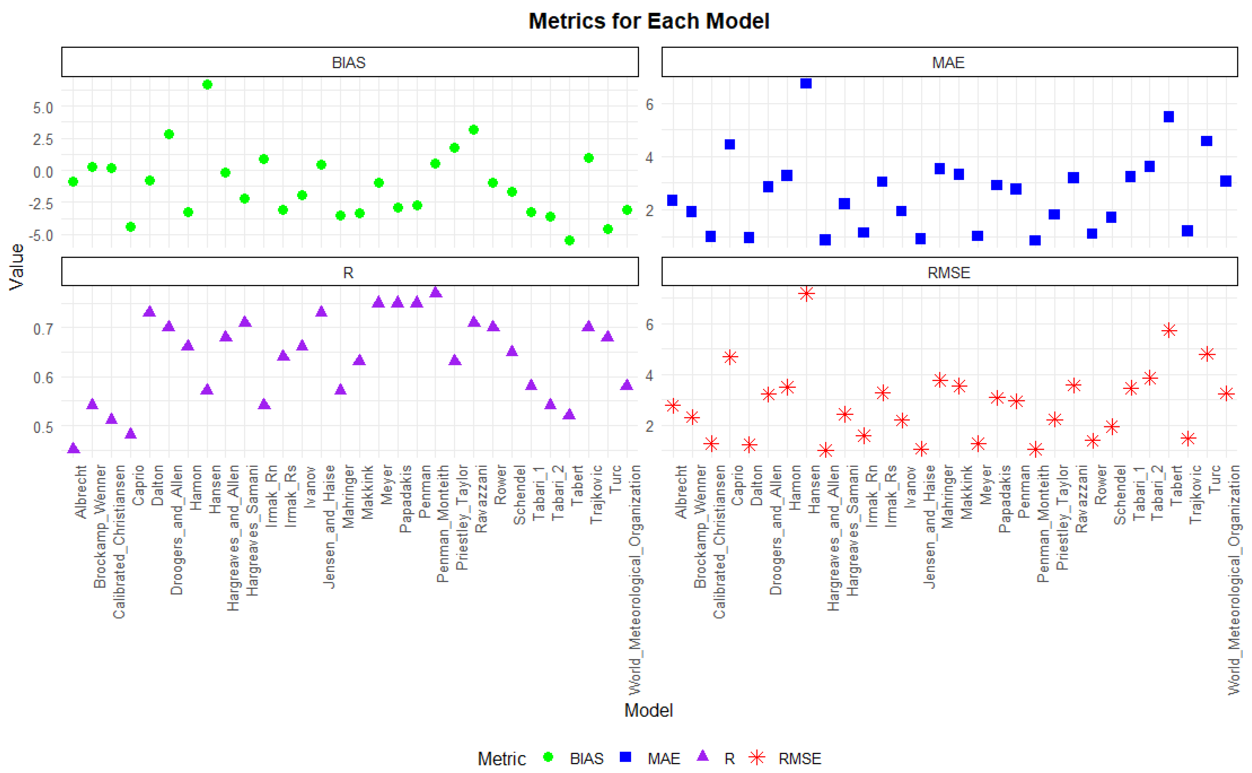
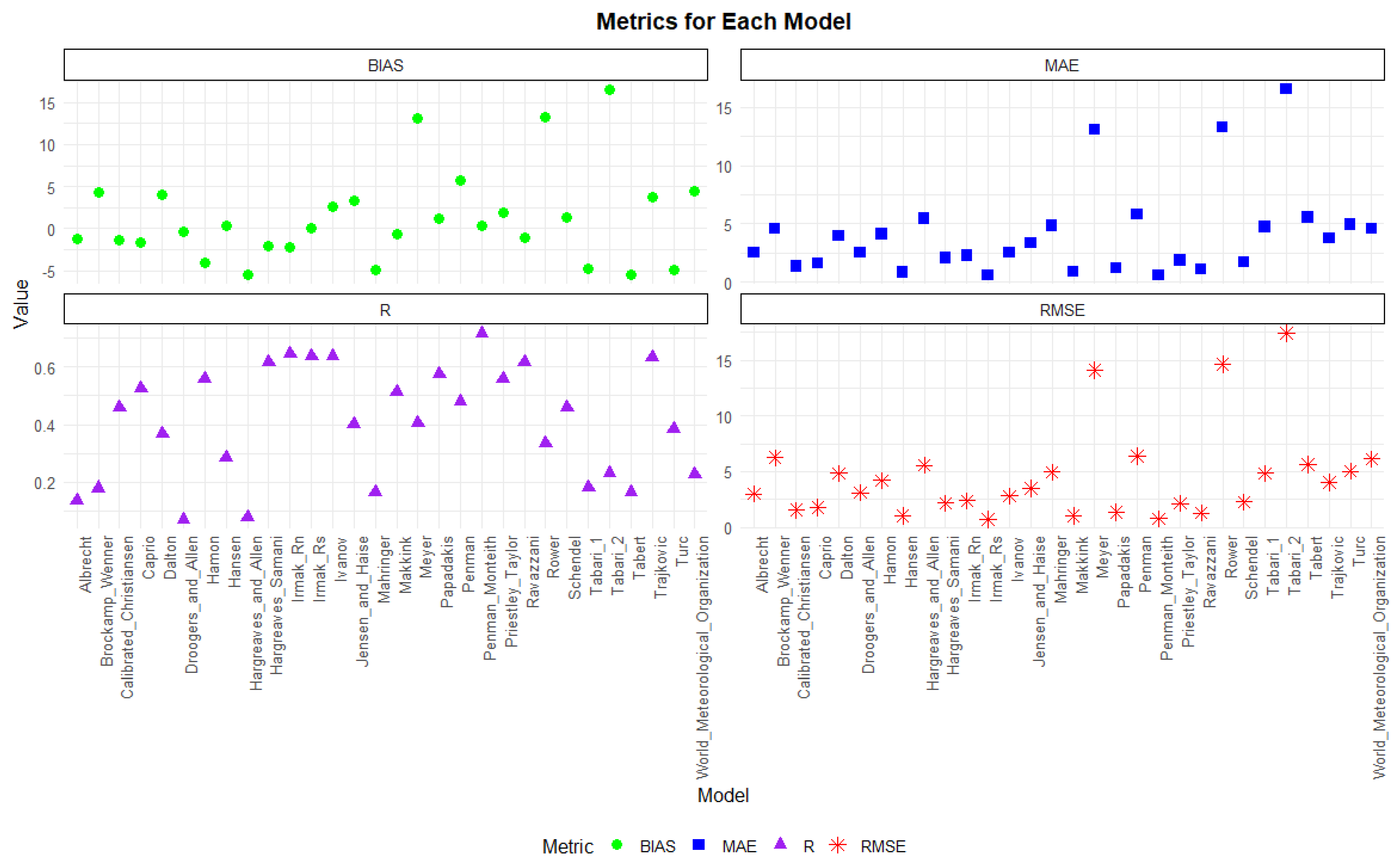
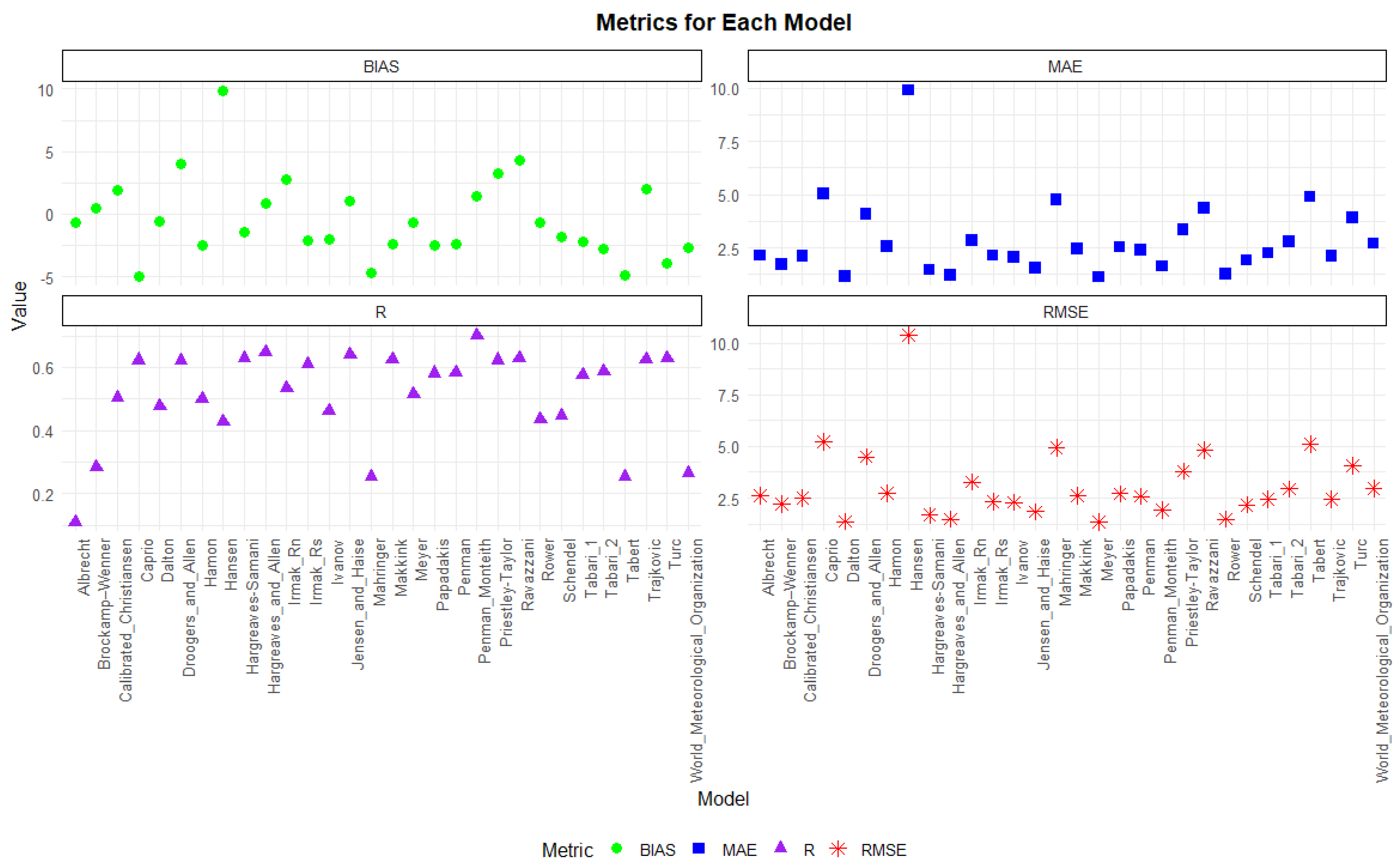
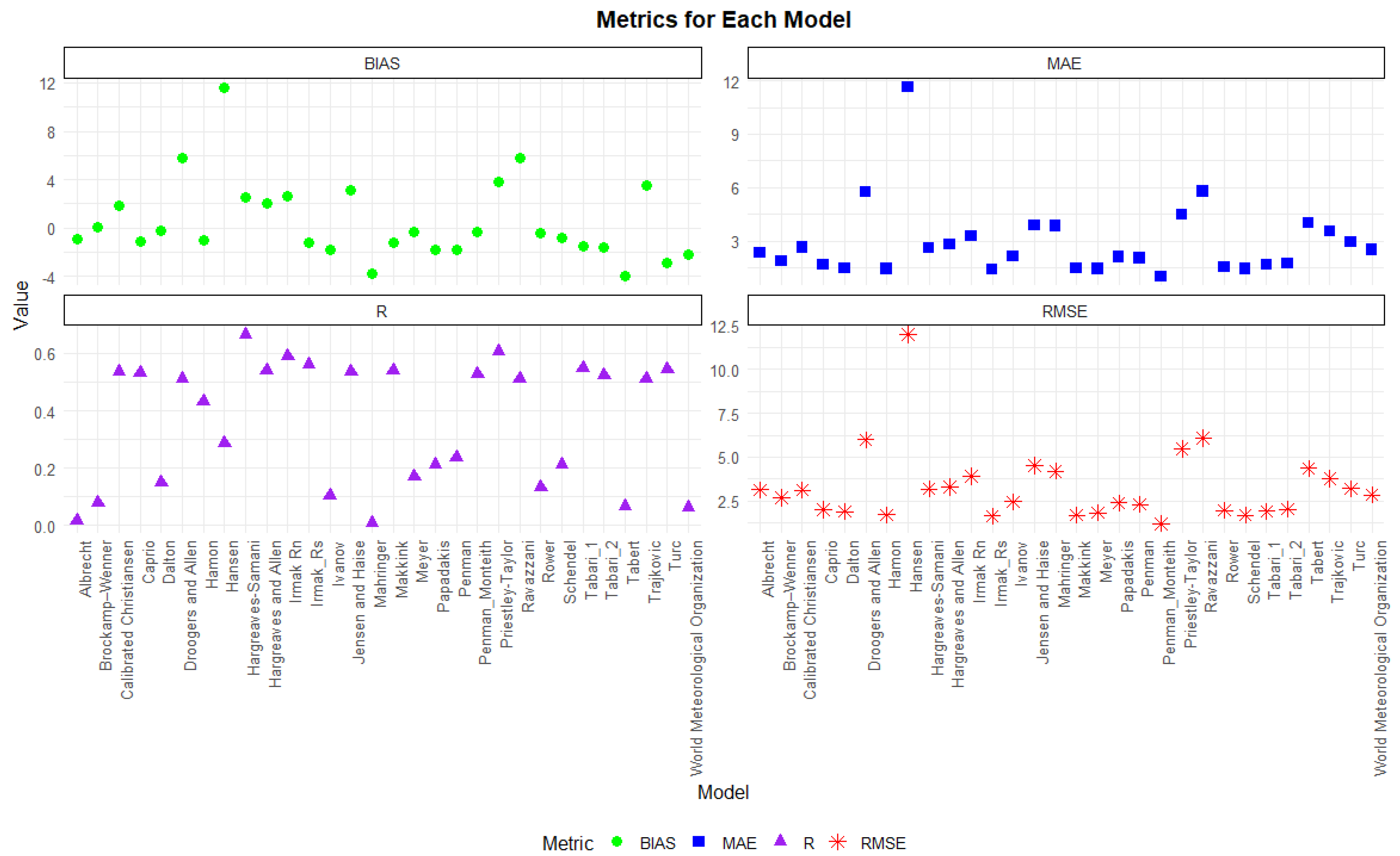
3.2. Comparative Analysis Between ETc Estimated from Different Micrometeorological Models and Lysimeter-Measured ETa

The comparative relationship between radiation-based models and lysimeter-measured ETa during the 2019 cropping season is demonstrated with scatterplots presented in Figure 3. The R² values represent the strength of the linear relationship between the estimated ETc and measured ETa values. The performance of the radiation models shows a clear hierarchy in terms of accuracy in the following order: Jensen and Haise > Turc > Irmark Rs = Priestley–Taylor = Makkink > Tabari 1 > Hansen > Tabari 2 = Irmark Rn > Calibrated Christiansen > Caprio. The Jensen and Haise model is the most accurate among the other models, with estimates that closely align with the lysimeter-measured ETa. The Turc model is slightly less precise but yields strong ETc estimates. The Irmak Rs, Priestley–Taylor, and Makkink models are equally accurate, with estimates closer to the ETa values, although they are not as precise as the Jensen and Haise or Turc models. The Tabari 1 model demonstrates a lower accuracy than the models behind it, whereas the Hansen model shows even less reliable ETc estimates. Furthermore, the Tabari 2 and Irmak Rn models show similar behaviors of low performance and accuracy, with estimates deviating further from the actual lysimeter measurements. The calibrated Christiansen model shows significant inaccuracies, whereas the Caprio model is the least accurate model, with poor results and the lowest R² value of 0.48.

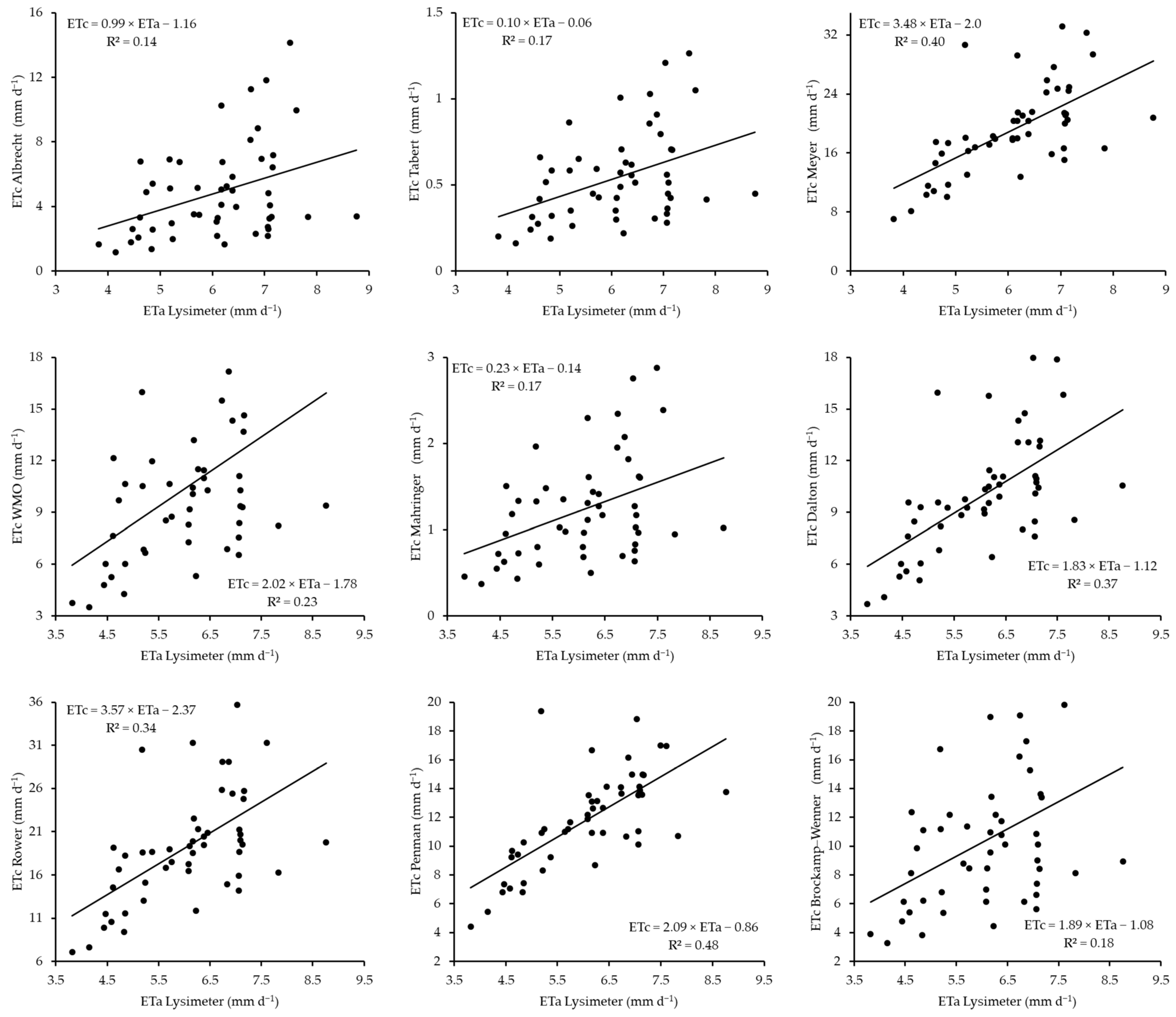
The scatterplots of the aerodynamic-based models for the 2019 cropping season, which demonstrate a comparison between the estimated ETc and measured ETa, are shown in Figure 4. The plots show a consistent positive correlation between the lysimeter ETa measurements and the different aerodynamic models that estimated ETc during this period, with resulting R² values ranging from 0.45 to 0.75, which indicates moderate to strong relationships. This resulted in the following model performance rankings from best to worst: Meyer = Penman > Dalton > Rower > WMO > Mahringer > Brockamp–Wenner > Trabert > Albrecht. Across these ranks, variations in the slopes and intercepts of the regression lines exist, suggesting different levels of agreement between the estimates by different models and lysimeter measurements. For example, the Albrecht and Brockamp–Wenner models demonstrate steeper slopes of 1.33 and 1.36, respectively, potentially over-estimating ETc at higher values, whereas models such as Trabert and Mahringer exhibit flatter slopes of 0.03 and 0.26, respectively, which are possibly under-estimating ETc values as the lysimeter ETa values increase. The Meyer, Dalton, and Rower models yielded slopes closer to 1, with values of 0.84, 0.91, and 0.92, respectively, which are in better agreement with the lysimeter ETa measurements, with R² values of 0.75, 0.73, and 0.7.

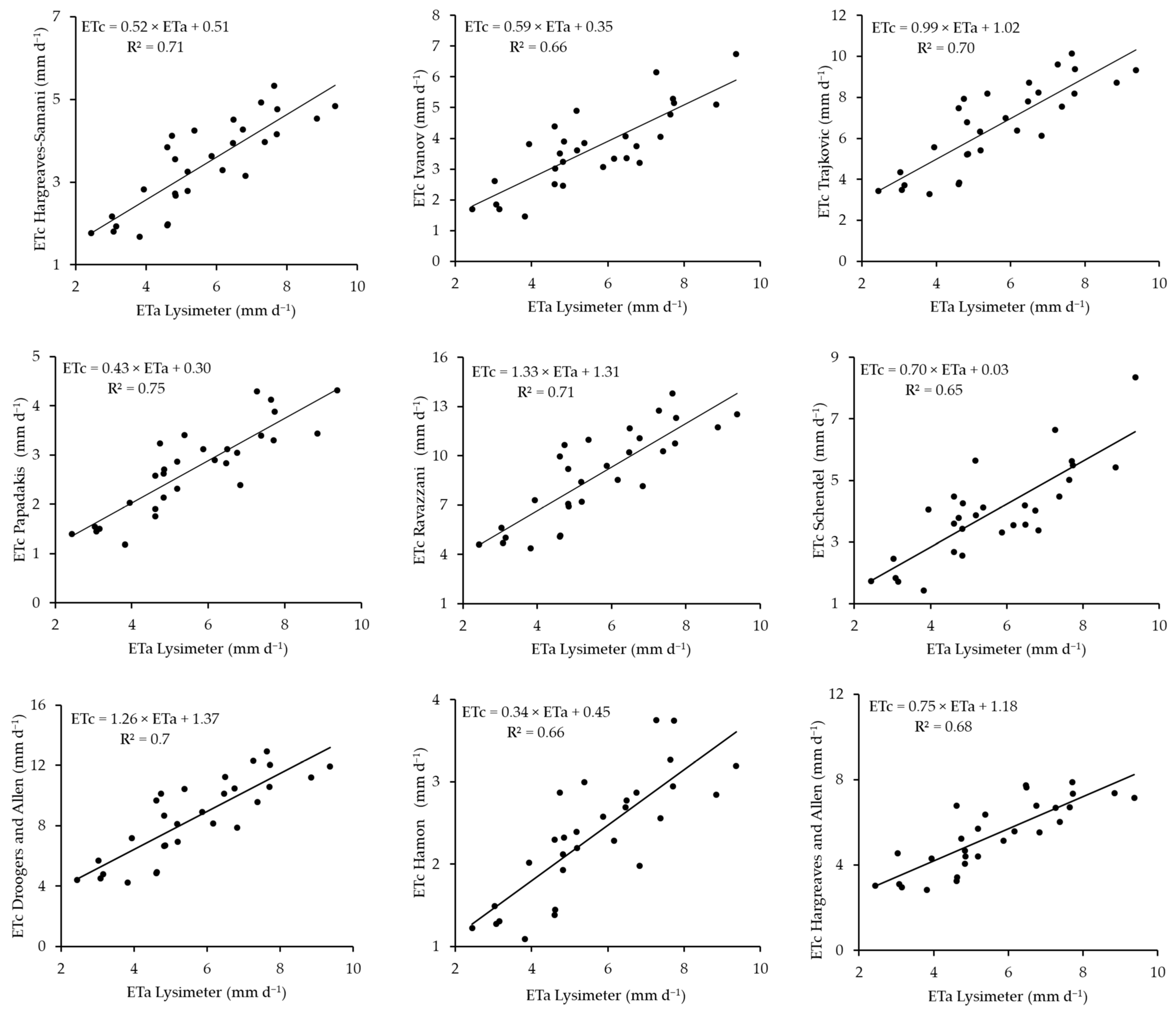
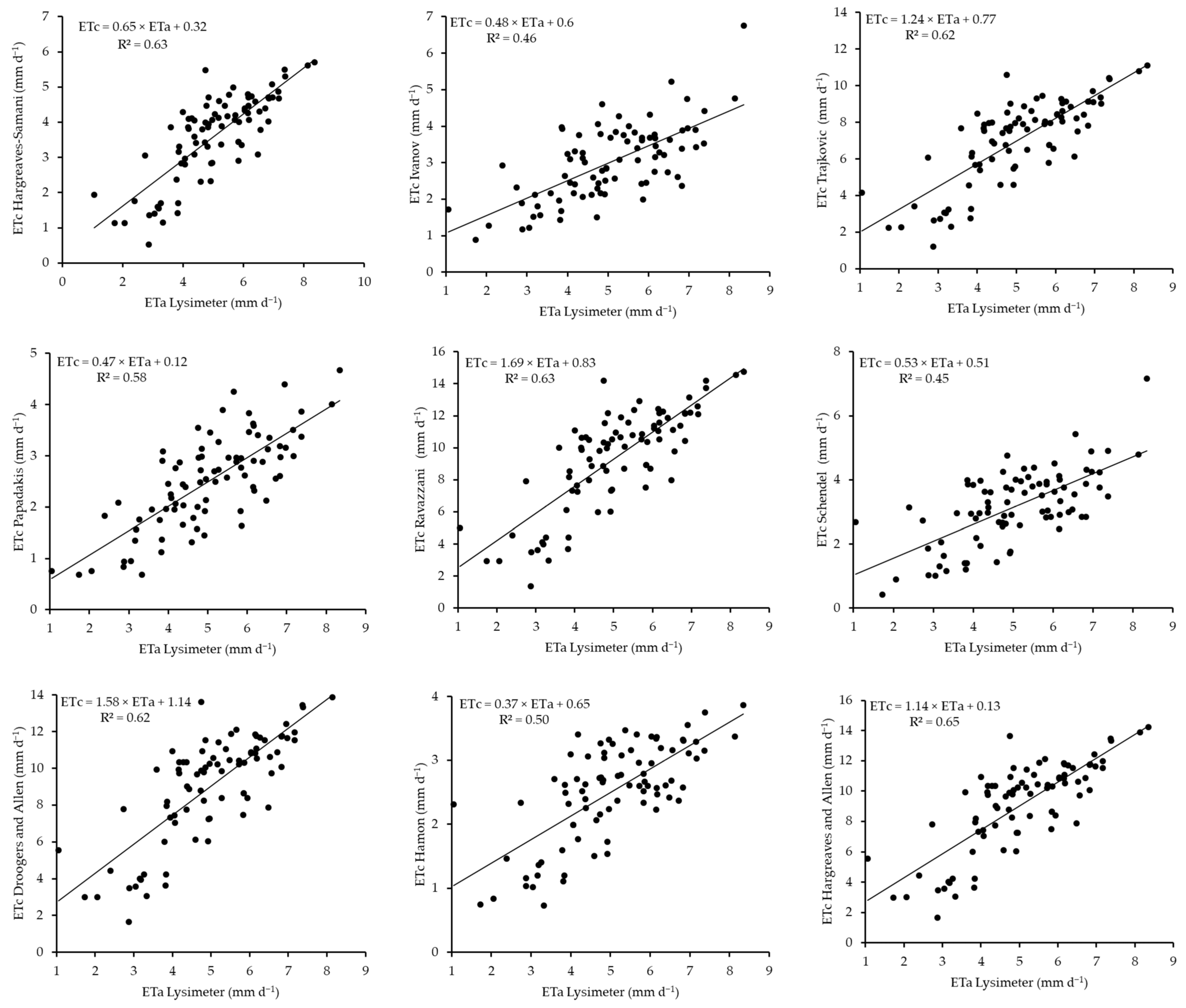
The comparisons between the temperature-based models for estimating ETc and lysimeter ETa are shown in Figure 5 for the 2019 barley cropping season. Similar to the other models, the R² values are used. The performances of these models are in the following order: Papadakis > Hargreaves–Samani = Ravazzani > Trajkovic = Droogers and Allen > Hargreaves and Allen > Ivanov = Hamon > Schendel. The rankings demonstrate the models’ performance based on their accuracy in estimating ETc. The Papadakis model, compared to the other models, appears to be the most accurate temperature-based model, providing estimates that closely match the ETa measurements. This is closely followed by the Hargreaves–Samani and Ravazzani models, which have similar levels of accuracy, although they are slightly lower than those of the Papadakis model. The Trajkovic model as well as the Droogers and Allen model follow; these models demonstrate comparable performances, with moderate accuracy. The Hargreaves and Allen model follows, with a reduced precision in estimating ETc compared with the other models. The Ivanov and Hamon models have the same level of accuracy, with reduced accuracy in estimating ETc. Lastly, the Schendel model yields the least accurate estimates, with an R² value of 0.65.

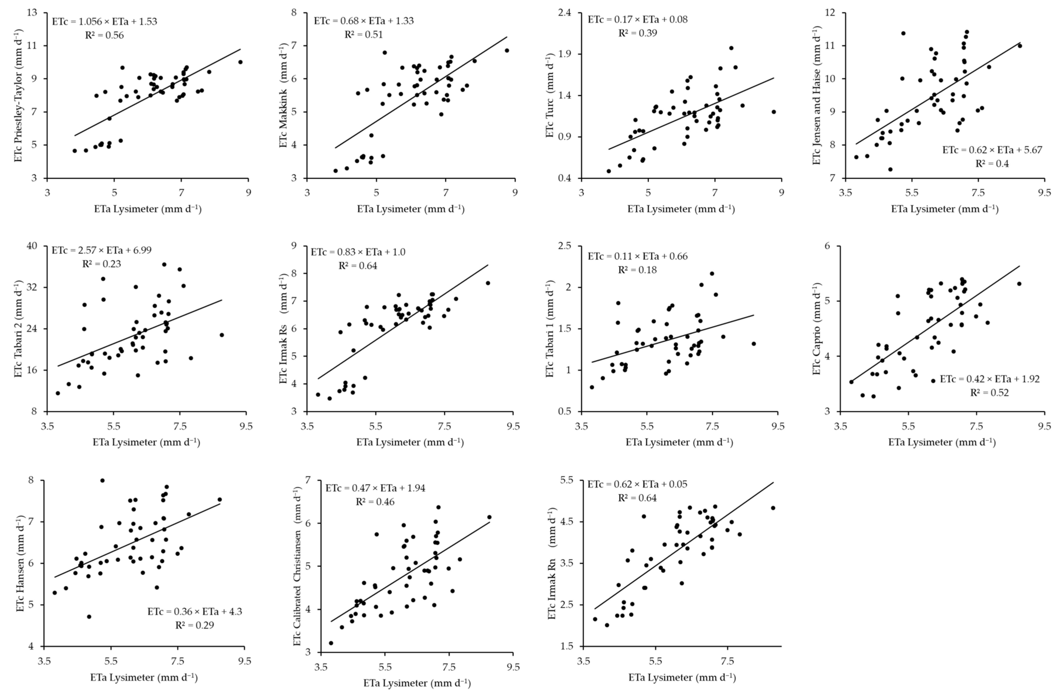
A comparison between the estimated ETc during the 2019–2020 cropping season using radiation models and the measured ETa is shown in Figure 6. Based on the R² values, the models are ranked in the following order: Irmark Rs = Irmark Rn > Priestley–Taylor > Caprio > Makkink > Calibrated Christiasen > Jensen and Haise > Turc > Hansen > Tabari 2 > Tabari 1. These rankings evaluate various models based on their accuracy in estimating ETc. The plots show that the Irmak Rs and Irmak Rn models performed similarly at the top of the rank, providing the most accurate estimates, with minimal deviation from the lysimeter ETa values. The model that closely follows these two models is the Priestley–Taylor model. This model also shows good performance, although it is slightly less accurate. The Caprio model then provides moderately accurate estimates. Following this model, the Makkink model demonstrated a lower accuracy than the models above it. The calibrated Christiansen model has a greater accuracy. Tabari 1 is at the bottom, providing the least accurate ETc estimates among the radiation-based models.

A comparison of the aerodynamic-based models for estimating ETc with ETa measured by the smart field weighing lysimeter from 2019–2020 is shown in Figure 7. Based on the R² values of the models, the models are ranked in the following order: Penman > Meyer > Dalton > Rower > WMO > Mahringer = Tabert = Brockamp–Wenner > Albrecht. On this basis, the Penman model leads with the highest accuracy, providing ETc estimates that are closer to the ETa measurements. The Meyer model provides slightly less accurate estimated values, but it still performs very well. Following Meyer, the Dalton and Rower models demonstrate moderate accuracy levels that are lower than those of Penman and Meyer. The Mahringer, Tabert, and Brockamp–Wenner models yield similar performances, with reduced accuracy. Finally, the Albrecht model ranks the lowest, providing the least accurate ETc estimates among the aerodynamic-based models, with an R² value of 0.14.

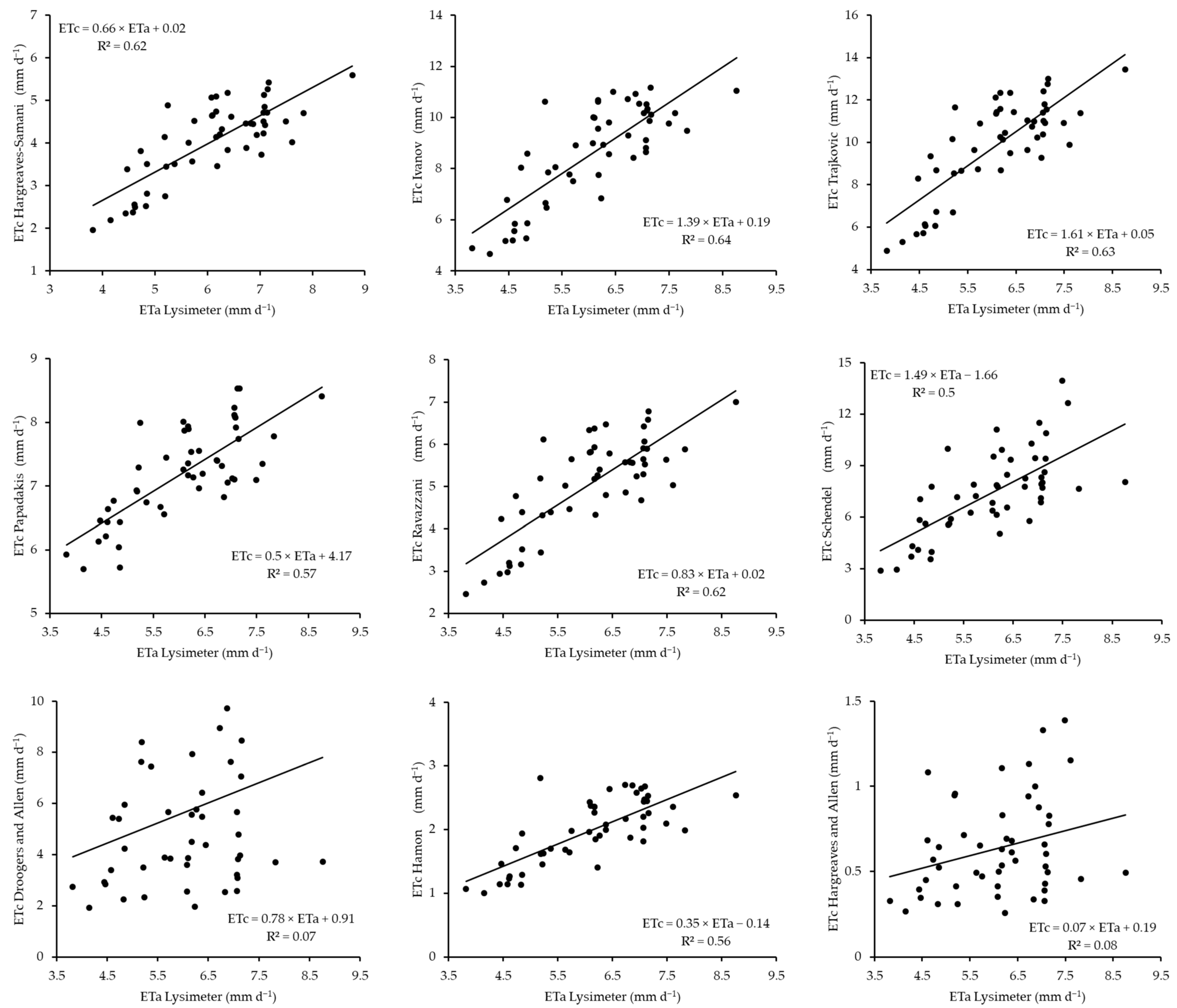
The scatterplots displayed in Figure 8 show the relationships between the ETc values estimated using different temperature-based models and the lysimeter-measured ETa values. These models are ranked from best to worst as follows: Ivanov > Trajkovic > Hargreaves–Saamani = Ravazzani > Papadakis > Hamon > Schendel > Hargreaves and Allen > Droogers and Allen. This reflects that the Ivanov model ranks first, providing the most accurate ETc estimates relative to the actual lysimeter measurements. The Trajkovic model yields slightly less accurate estimates, although it still performs well. Two models, Hargreaves–Saamani and Ravazzani, demonstrate similar performance levels, with moderate accuracy. On the other hand, the Papadakis model has a lower accuracy than the models above it. The Droogers and Allen models are at the bottom of the ranking hierarchy, offering the least accurate ETc estimates among the temperature-based models, resulting in an R² value of 0.07.

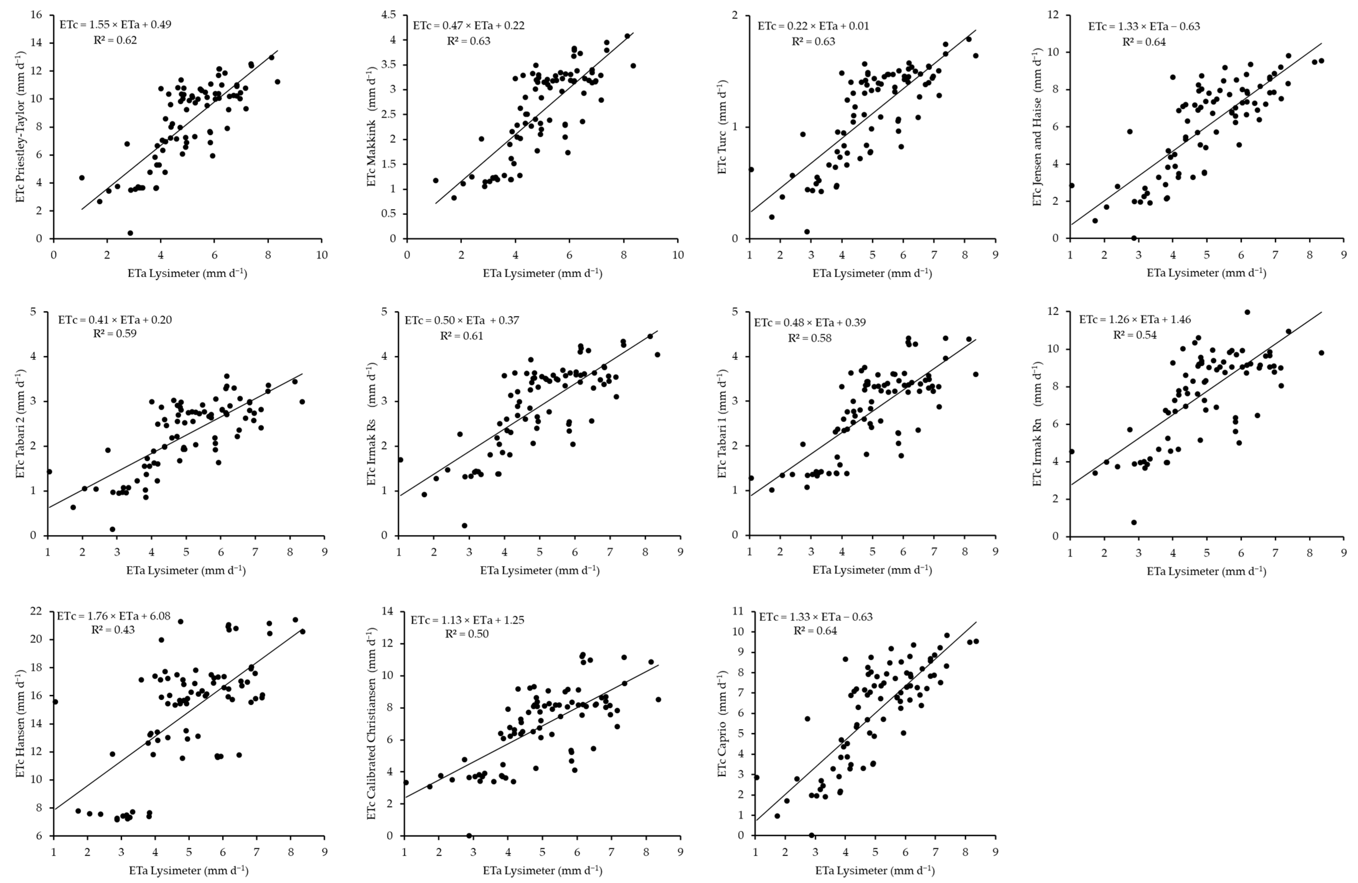
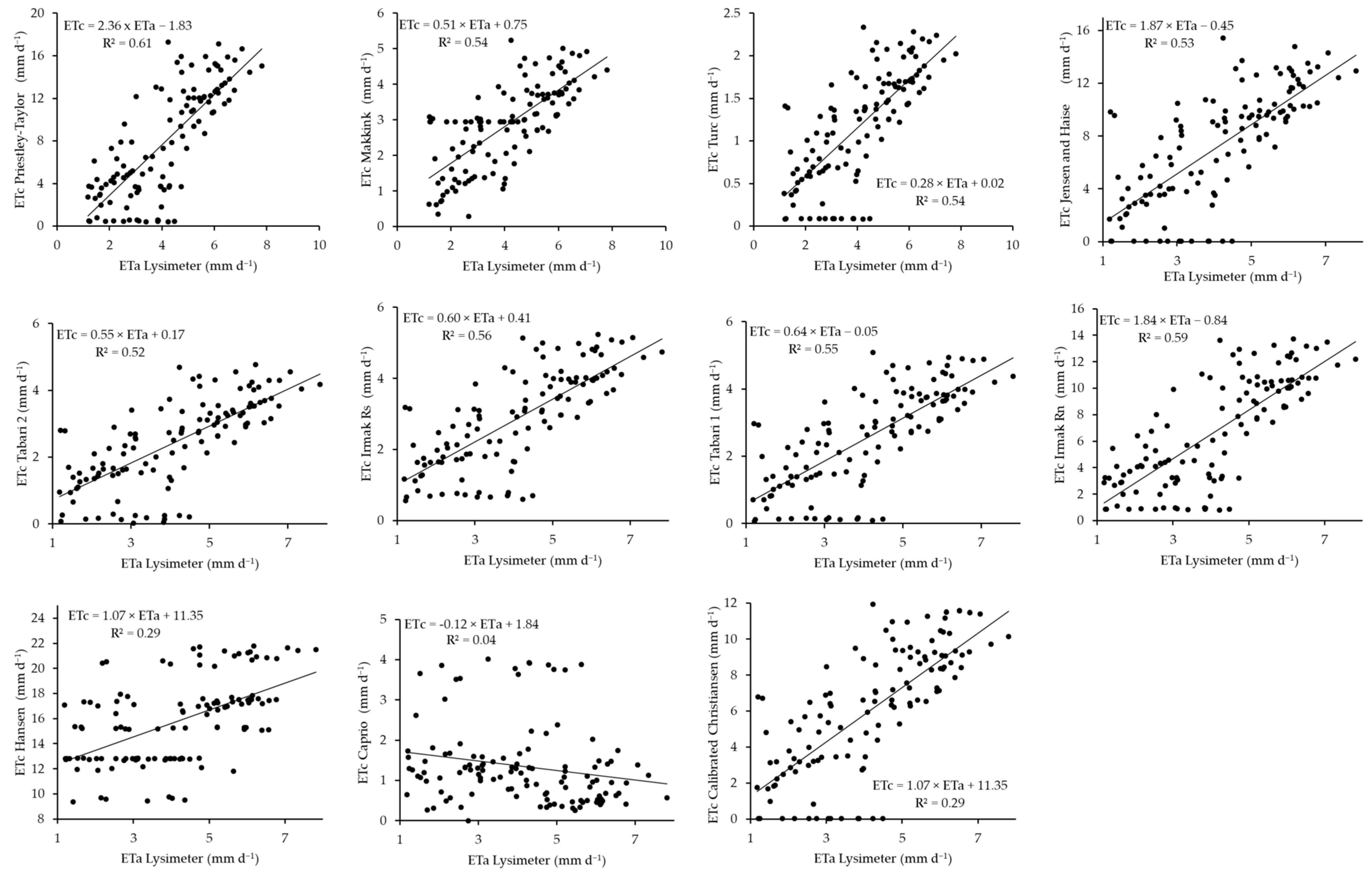
The 2020 winter barley cropping season estimates of ETc by different radiation-based models are presented in Figure 9. Based on the R² values, these models are ranked from best to worst in the following order: Jensen and Haise = Caprio > Turc = Makkink > Priestley–Taylor > Irmak Rs > Table 2 > Table 1 > Irmak Rn > calibrated Christiansen > Hansen. The Jensen and Haise models, along with the Caprio model, are in the upper part of the hierarchy and are the best-performing models for estimating ETc, providing values closer to the lysimeter ETa with minimal deviation. Following these models, the Turc and Makkink models demonstrate equal performance in estimating ETc with reduced accuracy, although they still perform well. The Priestley–Taylor model follows, with moderate accuracy. The Hansen model ranks at the bottom of the hierarchy, providing the least accurate ETc estimates among the other radiation-based models, with an R² value of 0.43.

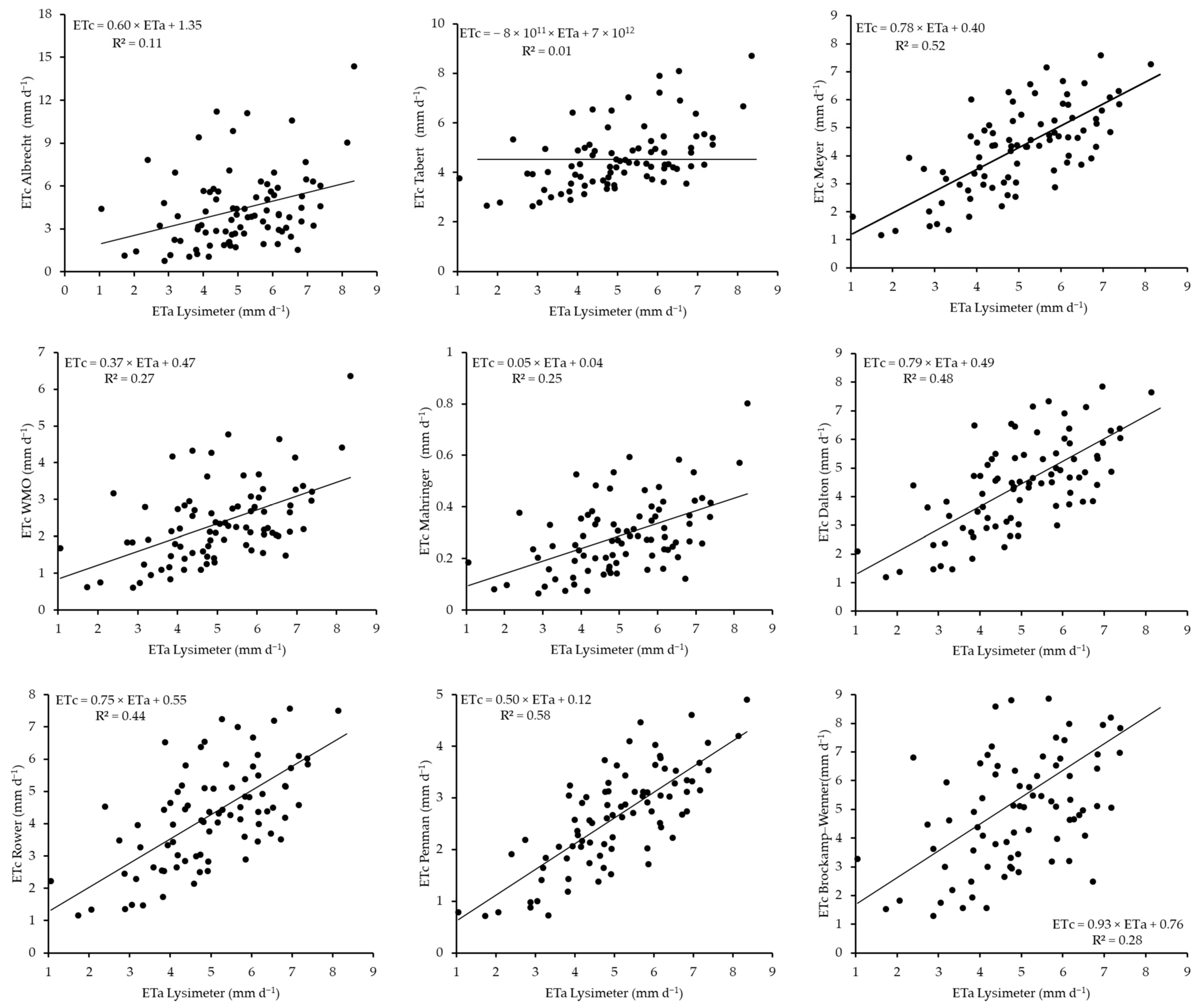
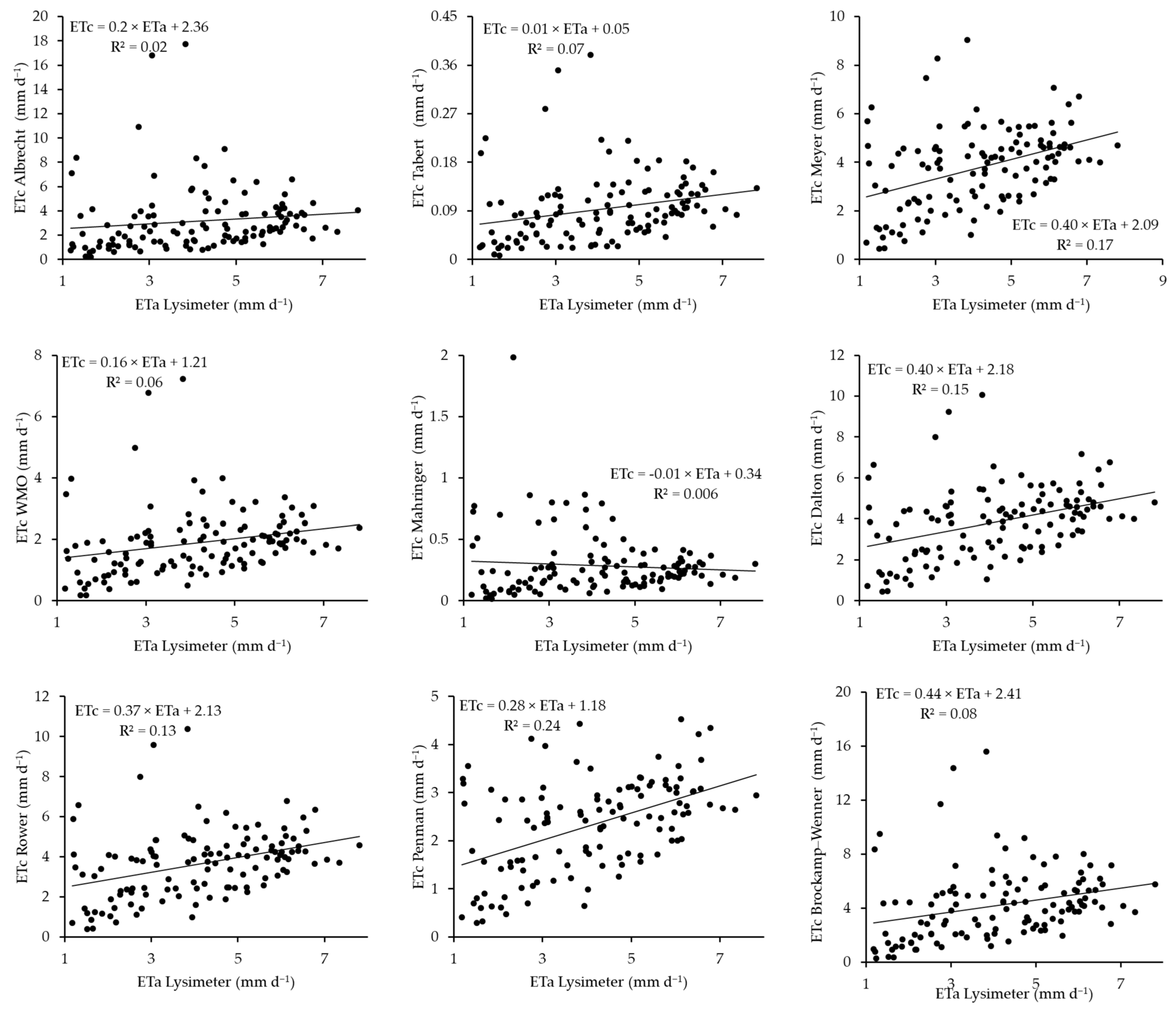
The scatterplots comparing ETc estimated by different aerodynamic models with ETa measured using a lysimeter are displayed in Figure 10. These models were ranked from best to worst for the 2020 winter barley season considering the R² value for each plot in the following order: Penman > Meyer > Dalton > Rower > WMO > Mahringer > Brockamp–Wenner > Albrecht > Tabert. The plots show that the Penman model is the most accurate model, providing estimates that are closest to the actual lysimeter measurements. Following that, Meyer’s model provides slightly less accurate estimates, although the performance is still good. The Dalton and Rower models have moderate accuracy levels that are lower than those of the Penman and Meyer models. Finally, in the hierarchy, the Tabert model is at the bottom rank, providing the least accurate estimates among the aerodynamic-based models.

The relationships between the ETc estimates of various temperature models and the ETa measurements obtained using a smart field weighing lysimeter during the 2020 winter barley cropping season are displayed in Figure 11, with each plot showing the regression slopes and R² values. Based on the R² values, the models are placed in a hierarchy from best to worst in the following order: Hargreaves and Allen > Hangreaves–Semani = Ravazzani = Drogers and Allen = Trajkovic > Papadakis > Hamon > Ivanov = Schendel. The Hargreaves and Allen model leads the hierarchy, providing estimates that are closest to the actual lysimeter values. Following this model, four models, Hargreaves–Semani, Ravazzani, Droogers and Allen, and Trajkovic, demonstrated similar performance levels, with slightly lower accuracy than Hargreaves and Allen. The Papadakis model then follows, with reduced accuracy in its ETc estimates. The Ivanov and Schendel models at the bottom of the hierarchy yield poor ETc estimates, which are farthest from the actual lysimeter measurements.

The radiation-based models successfully estimated ETc during the soybean cropping season in 2021 and were compared with the lysimeter measurements as shown in Figure 12. The comparison was based on linear regression scatterplots, with each plot indicating the slope and R² value. The models were hierarchically ranked from best to worst in the following order: Priestley–Taylor > Irmak Rn > Irmak Rs > Tabari 1 > Turc = Makkink > Jensen and Haise > Tabari 2 > Hansen = Calibrated Christiansen > Caprio. The Priestley–Taylor model is the most accurate model for demonstrating estimates that are closest to actual lysimeter field measurements. The Irmak Rn and Irmak Rs models also closely follow, which also indicates good performance, although they are slightly less accurate than the Priestley–Taylor model. Tabari 1 shows that the model has a moderate performance accuracy. However, the Turc and Makkink models have similar performance levels, whereas the Jensen and Haise models are less accurate than the models above. Finally, the Caprio model ranks last, which demonstrates the least accurate ETc estimates, which are further from the actual measurements obtained by the smart field weighing lysimeter.

A total of nine aerodynamic-based models used to estimate ETc during the 2021 cropping season were compared against the ETa measured at the field level using a smart field weighing lysimeter. Linear regression analysis was performed across all the models, as demonstrated in Figure 13, with their corresponding R² values reported. The comparison of the estimated values with the actual field-measured values revealed that these models were ranked from best to worst in the following order: Penman > Meyer > Dalton > Rower > WMO > Brockamp–Wenner > Tabert > Albrecht > Mahringer. In this hierarchy, the Penman model is the most accurate model, as its estimates are closely aligned with the actual field measurements. This is followed by Meyer’s model, which has a good performance, although it is slightly less accurate than the Penman model. The Brockamp–Wenner and Tabert models show similar performances, with low accuracy. At the bottom of the hierarchy is the Mahringer model, which yields the least accurate ETc estimates.

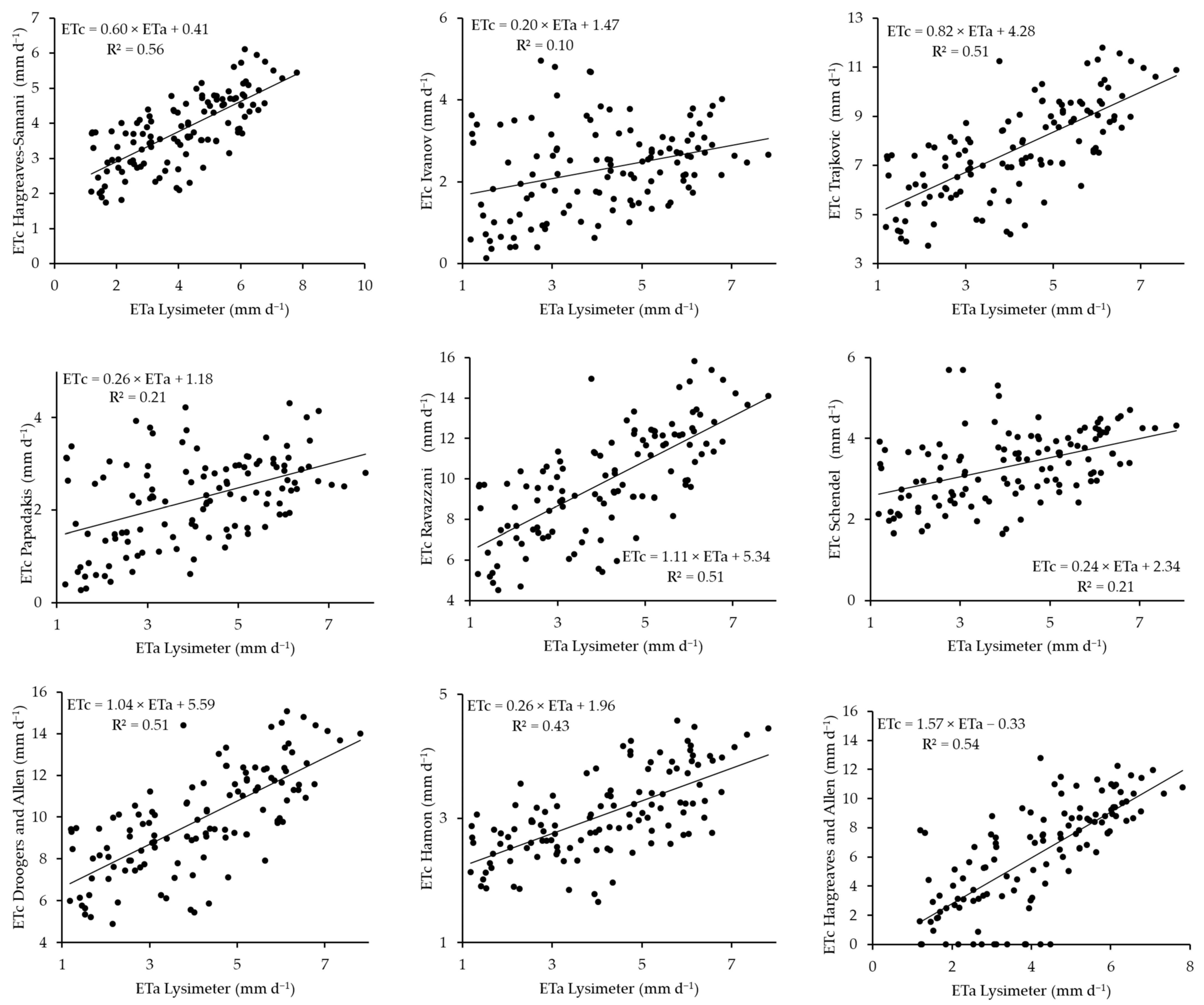
The scatterplots presented in Figure 14 demonstrate the performance of the different temperature-based models during the 2021 soybean cropping season. The model performances are ranked in the following order from best to worst: Hargreaves and Allen > Hagreaves–Saamani > Hamon > Trajkovic = Ravazzani = Droogers and Allen > Papadakis = Schendel > Ivanov. Among these models, the Hargreaves and Allen model performs best, with ETc estimates closer to the ETa values. This is followed closely by the Hargreaves–Samani and Hamon models, with less accurate estimates, although they are still better than the models below them. The Trajkovic, Ravazzani and Droogers, and Allen models have similar performances, showing moderate ETc estimation accuracy, whereas the Papadakis and Schendel models also exhibit comparable but less accurate ETc estimations. The Ivanov model ranks the lowest on the hierarchy, with the farthest deviation from the ETa measurements.

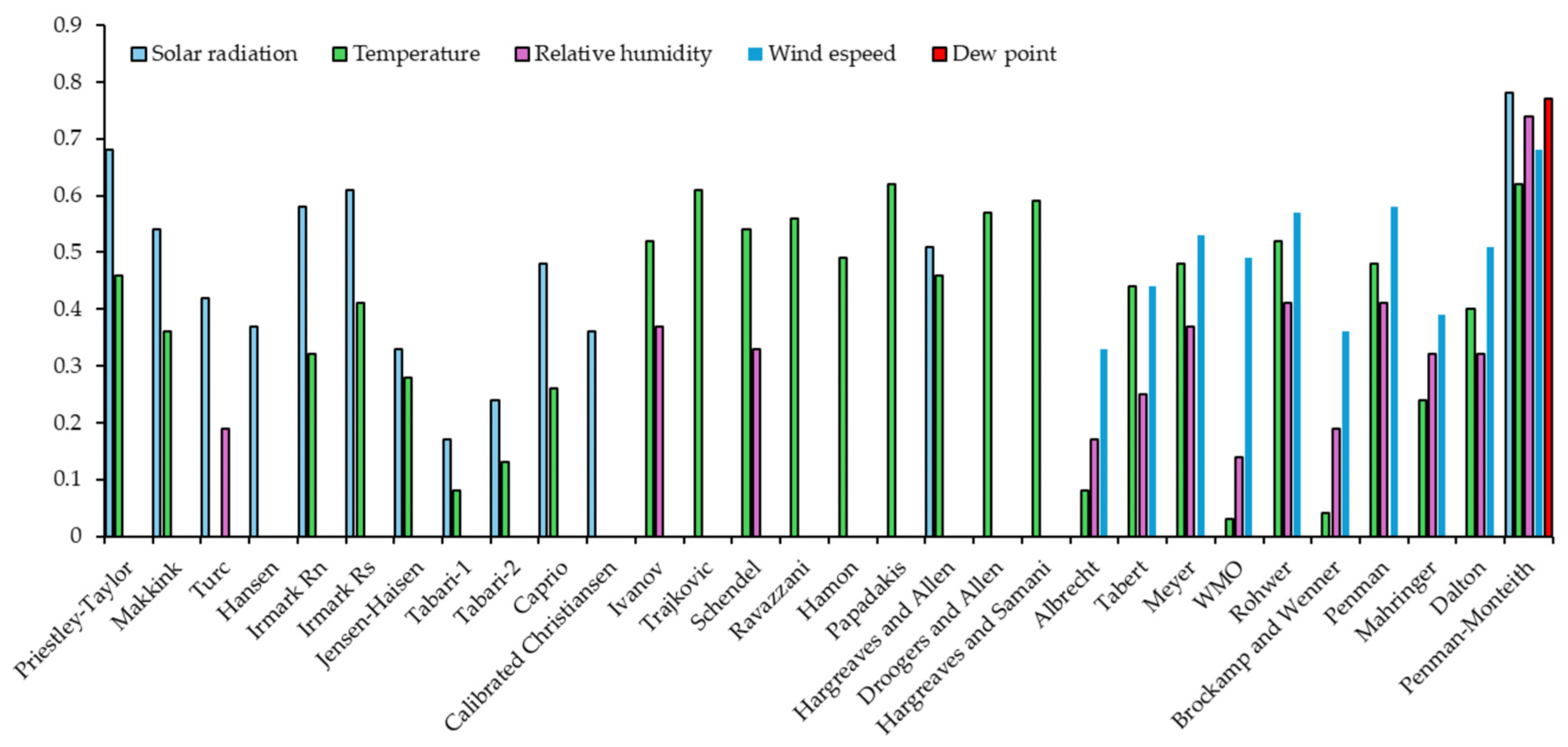
The Penman–Monteith model is a stand-alone model that combines radiation temperature and aerodynamic models. As a result, the comparison of this model’s estimation of ETc across different cropping seasons compared with the lysimeter ETa were separated from the other groups and are presented in Figure 15. The plots revealed that during the 2019 cropping season, the model estimated ETc the best, followed by the 2019–2020 maize season, with R² values of 0.77 and 0.72, respectively. During the 2020 winter barley season, the accuracy although good, decreased with an R² value of 0.7, whereas the lowest performance occurred during the 2021 soybean cropping season, with an R² value of 0.67, which is still moderate. However, when the Penman–Monteith model was compared with the other models in each category’s highest-performing models, this model outperformed all the other models in each season, as the R² values in 2019 ranged between 0.73 and 0.75, with the Penman–Monteith model resulting in an R² value of 0.77. For the 2019–2020 season, the R² range was between 0.48 and 0.64, whereas the Penman–Monteith method resulted in an R² value of 0.72. In the 2020 barley season, the R² values of the other models ranged between 0.58 and 0.65, whereas the Penman–Monteith model resulted in an R² value of 0.7. During the final soybean cropping season, the range of R² values among the models was between 0.24 and 0.61 among the best-performing models in each group, whereas the Penman–Monteith method resulted in an R² value of 0.67.

3.3. Evaluation Metrics Based on Comparisons Between Model-Estimated ETc and Lysimeter-Measured ETa

The statistical metrics output when 30 micrometeorological model estimates for ETc were compared with those for ETa for the four seasons are presented in Figure 16, Figure 17, Figure 18 and Figure 19. The green circles represent the bias, while the blue filled boxes resemble the MAE. The purple, pyramid-shaped marks represent the correlation coefficient (r) values, and the orange stars represent the RMSE values. Figure 16, Figure 17, Figure 18 and Figure 19 demonstrate some degree of overestimation and underestimation. These findings in certain seasons can be attributed to their sensitivity to dominant climatic factors. For example, radiation-based models tend to overestimate ETc during seasons with high solar radiation due to their reliance on temperature and solar inputs [55,56]. On the contrary, aerodynamic models may underperform in conditions with low wind speeds, as they are heavily influenced by air movement [57]. Seasonal variability in rainfall, humidity, and crop growth stages also affect model accuracy. For instance, during dry winter seasons, models that inadequately account for soil moisture content may underestimate ETc. Understanding these limitations emphasizes the importance of directing model selection towards seasonal climatic conditions and crop water requirements.

3.3.1. Evaluation Metrics for the 2019 Cropping Season Estimates

The statistical metrics used to evaluate the different models during the 2019 winter barley cropping season are shown in Figure 16. During this season, the Penman–Monteith model showed a bias value just above zero, indicating a slight overestimation of ETc. The Jansen and Haise models show similar biases, whereas the Tabari 1 model shows a negative bias below 0, indicating an underestimation of ETc, whereas Caprio and Tabari 2 show the most negative bias values, which are related to an underestimation of ETc. The Hansen model shows the most positive bias, approaching 6, demonstrating ETc over-estimation. The errors, which include the MAEs and RMSEs, appear to be minimal for the Penman–Monteith, Meyer, Dalton, and calibrated Christiansen models. There are good correlations in some model estimates of ETc compared with those of the lysimeter ETa, as demonstrated by the high r values. These models include the Penman–Monteith, Meyer, Papadakis, Trajkovic, and Makkink models, with the Penman–Monteith model achieving the highest correlations with the measured ETa values. Although the Penman–Monteith shows good correlations, other models such as Penman, Papadakis, Meyer, and Dalton also demonstrate good correlations, suggesting that they can be used as an alternative under such seasonal and crop conditions. The overestimation and underestimation observed could be linked to the inherent parametrization of the evaluated models and their sensitivity to seasonal meteorological conditions. For example, the Penman–Monteith model, with a bias slightly above zero, slightly overestimates ETc. This overestimation can be attributed to its sensitivity to solar radiation and temperature, which might be higher than actual winter conditions warrant. Similarly, the Hansen model, which shows the most positive bias (approaching 6), overestimates ETc likely due to an over-reliance on temperature or an amplification of the limited energy available in winter. On the other hand, models such as Tabari 1, Caprio, and Tabari 2 exhibit negative biases, indicating an underestimation of ETc. This underperformance could emerge from the simplified model structures that inadequately capture the reduced energy inputs and complex microclimatic conditions associated with the winter season. As a result, these models may lack mechanisms to account for localized variations in net radiation or soil heat flux, leading to lower ETc estimates.

3.3.2. Evaluation Metrics for the 2019–2020 Cropping Season Estimates

During the 2019–2020 maize cropping season, the statistical metrics shown in Figure 17 demonstrated minimal errors, including Irmak Rs, Penman, Hansen, and Penman–Monteith. Higher correlations were achieved by the Penman–Monteith, Irmak Rs, and the Hargreaves and Samani models. In terms of bias, the Irmak Rs and the Penman–Monteith models appear near zero, which shows minimal differences between the estimated ETc and measured ETa values. These findings suggest that, in situations where the applicability of the Penman–Monteith is not practical possibly due to limited data availability, models such as the Irmak Rs, Meyer, and Papadakis can be used as alternatives. The model overperformance may emerge from the parameterization and calibration to the local climatic data of the models, while the underperformance in other seasons may be due to limited consideration of certain meteorological variables such as wind speed or vapor pressure deficits, which become more critical in seasons with higher variability, such as summer. For instance, models like Hargreaves and Samani might have underperformed in seasons where factors beyond temperature, such as solar radiation or soil moisture limitations, play a more significant role. Simpler models may excel under stable and predictable weather patterns.

3.3.3. Evaluation Metrics for the 2020 Cropping Season Estimates

The statistical metrics for the 2020 winter barely cropping season are shown in Figure 18, with bias, MAE, RMSE, and r values. The best-performing models based on these metrics are the Penman–Monteith model; Meyer, Jensen and Haise; and Hargreaves and Allen, with minimal errors, bias, and high correlations. The Penman–Monteith method appears to have the least errors with high correlation coefficient values among all the models. The Penman–Monteith model consistently outperformed the others due to its consideration of multiple meteorological variables. This versatility makes it highly reliable in capturing the reduced ETc dynamics during winter when energy inputs are lower. The Meyer and Jensen and Haise models also performed well, likely because they incorporate solar radiation and temperature, which remain the dominant factors even in colder seasons. The underestimation of the other models could be attributed to their reliance on simplified assumptions or exclusion of key meteorological variables relevant during winter. For example, temperature-based models like Hargreaves and Samani might overestimate ET on sunny winter days due to their high sensitivity to temperature without adequately accounting for the reduced vapor pressure deficit and aerodynamic resistance. Similarly, empirical models calibrated for summer conditions may not translate well to winter conditions, leading to higher errors. Models such as Trajkovic, Priestley–Taylor, Irmak Rs, Irmak Rn and Hargreaves and Samani, Hargreaves and Allen, and the Meyer model demonstrated good performance, which implies that they can be used as alternative models.

3.3.4. Evaluation Metrics of the 2021 Cropping Season Estimates

A comparison between ETc and ETa during the 2021 season, when soybean was the crop of the season, based on statistical metrics is shown in Figure 19. The statistics demonstrate that the Penman–Monteith model was the best-performing model across the season, with the lowest RMSE and MAE values. A slightly negative bias indicates minimal underestimation of ETc values with a moderate value of r, making it the most accurate among the compared models. The Priestley–Taylor, Hargreaves, and Allen models demonstrate good performances, with low errors and good correlations. However, the Hansen model has the highest RMSE and MAE, with a substantial positive bias and a weak r value, which indicates its poor estimation capability. The positive bias of approximately 11.63 is significantly greater than that predicted by the Hansen model, indicating that it consistently predicts values much higher than the actual measured values. The model might overestimate the influence of variables such as solar radiation or temperature, which are key drivers of evapotranspiration. If actual ETa is limited by factors like low soil moisture or high relative humidity, the model would still predict higher values based on its assumptions. Although the Penman–Monteith model has good performance, alternative models such as the Hargreaves and Samani, Dalton, Irmark Rs, Irmark Rn, and Makkink also demonstrate good performance during this season. This can be applied if similar environmental settings lack the full datasets to complete the Penman–Monteith model.

3.4. Model Ranking Across Different Seasons Based on Metric Scores

The overall rankings of the models across different seasons are presented in Figure 20, which shows the performance rankings of the various micrometeorological models in estimating ETc when they are compared with the measured field ETa. According to the rankings, the Penman–Monteith model stands out as the top-performing model, consistently ranking high in three seasons, with ranks of 1, 1, 4, and 1 in the 2019, 2019–2020, 2020 and 2021 seasons, respectively, and the lowest average rank of 1.75. Models such as Irmak Rs and Jensen and Haise show variable performance; for example, Irmak Rs excels in seasons 2 and 4 but falls significantly in seasons 1 and 3, which results in an average rank score of 8.75. The Jensen and Haise model performs exceptionally well in Seasons 1 and 3 but decreases in Season 4, which leads to an average rank of 11.75. The Meyer, calibrated Christiansen, and Makkink models demonstrate strong performance but have occasional dips. Moreover, models such as the Hansen and Tabert models consistently rank lower across all seasons, with average rank scores of 23.75 and 29, respectively, which indicate poor performance. The Hargreaves–Samani and Dalton models maintain relatively good ranks, although they experience occasional variability. The Schendel and Ivanov models exhibit stable performance, with moderate ranks in each season. The Trajkovic, Papadakis, and Brockamp–Wenner models perform well in some seasons, although they are inconsistent. The World Meteorological Organization, Droogers and Allen, and Turc models have consistently lower ranks, which indicates less-effective performance across the seasons.

3.5. Rankings of Micrometeorological Models

The rankings of the models for estimating ETc in comparison with ETa measured by a lysimeter reveal that the Penman–Monteith model is the most accurate, followed by Irmak Rs and Schendel, which also provide close estimates (Figure 21). Models such as Dalton, Hargreaves–Samani, and Meyer perform reasonably well, whereas mid-ranked models such as Makkink and Jensen and Haise show moderate accuracy. The lower-ranked models, including the Irmak Rn, Hamon, and traditional Penman models, demonstrate significant discrepancies. The least-accurate models, such as the World Meteorological Organization model and the Tabert model, exhibit substantial deviations from the actual ETa values, indicating less reliability in estimating ETc. Most models show seasonal variability in performance; although they do not reflect ETc accurately in some seasons, they are still usable in seasons where their data requirements are favorable. This is important in areas where the applicability of the Penman–Monteith model is not practical due to input data constraints.

3.6. Comparison Between Model Estimates and Measured Lysimeter Seasonal ETa

Table 7. Comparative analysis of different models for estimating ETc across seasons.

		Season 1	Season 2	Season 3	Season 4
Model Group	Model/Measurement	ETc Barley (mm)	ETc Maize (mm)	ETc Barley (mm)	ETc Soybean (mm)
Field data	Lysimeter ETa	162.83	304.64	422.83	494.19
Combination	Penman–Monteith	178.33	323.63	455.27	458.09
Temperature	Schendel	118.68	372.23	365.9	398.5
Aerodynamic	Dalton	124.53	402.86	375.48	390.26
Radiation	Irmak Rs	140.81	304.49	384.13	446.89

lists the ETa and ETc values measured by the lysimeter and estimated by the top-performing models for each class of ETo model. The lysimeter values here are used as a benchmark for barley, maize, and soybean crops against the ETc models (Penman–Monteith, Schendel, Dalton, and Irmak Rs). The comparison in terms of which model estimates ETc with values closer to the lysimeter ETa measurements on the ground reveals that the Penman–Monteith model provides ETc estimates closer to the lysimeter ETa measurements for barley in both seasons and the maize crop, whereas it shows an over-estimated ETc in the soybean cropping season. On the other hand, the Schendel and Dalton models have greater differences between the modeled ETc and measured ETa. The Irmak Rs model provides estimates of ETc that are reasonably closer to the lysimeter-measured ETa values for some crops and seasons, rendering them reliable under some conditions. Although the Penman–Montieth model provides estimates closer to those measured by the lysimeter, its applicability can be limited by its high volume of data required. In data-scarce environments, alternative models such as Irmark can be used for favorable seasons when it performs better.

3.7. Analysis of Meteorological Variables’ Impact on Estimated ETc by Different Models

A detailed analysis of meteorological influence on ETc estimation across different seasons from different modes is depicted in Figure 22. The figure shows an average Pearson correlation coefficient from four cropping seasons relating estimated ETc with solar radiation, temperature, relative humidity, wind speed, and dew point. Across the radiation models, solar radiation is the primary driver of ETc; however, during the winter season, this variable is normally low. As a result, the influence of solar radiation may be reduced, although it still dominates the process of ETc as radiation-based model input. On the other hand, during winter, temperatures are also normally low, and the influence of temperature might be reduced as the vapor pressure deficit decreases. Solar radiation and temperature appear to be the dominant factors influencing ETc across most models, with solar radiation exhibiting the strongest correlation. This is evident in energy-based models like Priestley–Taylor and Penman–Monteith. Temperature also has a significant impact, especially on temperature-driven models like Hargreaves and Allen, where it affects the vapor pressure deficit and ET potential. Relative humidity and wind speed show moderate to weak correlations, while wind speed played a more prominent role in aerodynamic models and relative humidity, inversely influencing ETc by reducing the vapor pressure deficit. Dew point has the weakest correlation, reflecting its limited role as a direct driver of ETc. In winter, reduced solar radiation and temperature diminish ETc, making energy-based models more reliable, while in summer, higher solar radiation and temperature amplify ETc, highlighting the importance of these variables.

4. Discussion

The importance of saving water has long been emphasized to support and achieve the sustainable development goals set by the United Nations. In agriculture, more water is used and wasted on irrigation, which requires immediate intervention by introducing accurate and timely water applications. The only practical approach to solve this problem is to accurately understand how much water is lost after each irrigation. To achieve this with limited direct measurements of crop water use devices, accurate models to quantify ET are needed. This study evaluated 30 micrometeorological models to estimate ETc, which were compared with ETa values from a smart field weighing lysimeter. This was necessary in this study because none of these models were developed in South Africa, and they have mostly been used for estimating ETo. For most applications in South Africa, these models have been evaluated using the standard Food and Agriculture Organization (FAO) Penman–Monteith model. None of the evaluations have been performed using a smart field lysimeter or data with high accuracy for determining ETc.

Moreover, the determination of ETc is based on integrating Kc values, which are crop-specific to ETo, and adjusting Kc values is important to avoid errors in irrigation timing, which can compromise crop yields. Ko et al. [58] noted that variations in temperature, humidity, and crop development can significantly impact Kc values. The study findings on the determination of local Kc values compared with the published Kc values by the FAO for barley, maize, and soybean demonstrated disparities in some crop stages, emphasizing the fact that Kc values can vary from one region to another, which could induce errors in ETc, resulting in the water being used not matching the required amounts. Previous studies, such as those by Tarantino and Onofrii [59] and Doorenbos and William [60], emphasized that there are mostly discrepancies between locally derived Kc values and those published by the FAO when experiments are conducted, which supports the notion of crop locality-specific adjustments of Kc values. In this study, the initial Kc values, which ranged from 0.32 to 0.46 during the germination stages, indicated that these crops used only 32% to 46% of the water required by a reference crop. This can be attributed to the small leaf surface area and significant soil water evaporation during the early growth stages. As the crops advanced to the midseason stages, their demand for water increased, which was reflected by their Kc values ranging from 1.12 to 1.18. This peak can be attributed to the increase in leaf surface area and transpiration rates, which demonstrated the critical crop growth period that necessitated additional water between 12% and 18%. Moreover, as these crops matured and approached senescence stages, the Kc values decreased to values between 0.22 and 0.47, which could have been a sign of a reduction in water demand as the crops were preparing for harvest and naturally drying out.

While the main objective of this study was to evaluate several ETc estimation models following the successful determination of locally derived Kc values, the results demonstrated variable performance of different models, revealing instances of both overestimation and underestimation of ETc across all seasons, reflected in the regression scatterplots and the bias values. The variability in performance has been reported in the study by Bakhtiari et al. [61], who used a lysimeter to evaluate six models in arid environments in Iran. This variability suggests several critical insights into each model’s performance, reliability, and applicability under different climatic and farm management conditions [2]. The occurrence of both overestimation and underestimation of ETc indicates that most models cannot consistently provide accurate ETc estimates for each season with different climate conditions. This variability can be attributed to the differences in the structure of different models and the specific climatic parameters they incorporate when estimating ETc [62,63]. Models such as the Penman–Monteith model require more meteorological data, which are not always available in most regions, particularly in developing countries with limited stations [23]. However, in the study area, the model might have performed well because data were available but might not yield the same results when data are scarce or less accurate. A study conducted by Córdova et al. [64] supports such suggestions, observing that the accuracy of ETo calculations based on the Penman–Monteith model decreased as the number of missing variables increased, with significant overestimations observed when key parameters such as solar radiation were inadequately represented. This explains why other models have been developed that require limited data [65,66]. However, ET is not a single variable component; it has variables which change, requiring models that can capture different elements that contribute to ETc. The overestimation of ETc in some models suggests that these models might be overly sensitive to certain climatic inputs, leading to higher water use predictions than those experienced in the field [67]. For example, radiation-based models that estimate ETc based on solar radiation or temperature might overestimate ETc in seasons where these factors are particularly intense. This suggests that models sensitive to specific climatic inputs may yield higher water use predictions than what is observed in practice, leading to inefficient water use, over irrigation, increased water waste, and potential negative impacts on crop health and soil conditions. On the other hand, the underestimation of ETc by some models suggests that they might not fully capture the actual crop water requirements under certain conditions. This could be due to models underestimating factors such as wind speed, humidity, or specific crop stress responses [68]. Underestimation can lead to under-irrigation, stressing crops and potentially reducing yields.

The seasonal variability in model performance further emphasizes the complexity of accurately predicting ETc. Each season presents different climatic conditions, such as varying temperatures, rainfall patterns, irrigation amounts, and sunshine hours, which can impact model accuracy [69,70,71]. As a result, the study findings demonstrated that models that perform well in one season might not necessarily do so in another, indicating that their calibration might be season-specific or that they require adjustments for different times of the year. For example, while the Penman–Monteith model demonstrated good performance, as evidenced by the ranking, the Irmark Rs model demonstrated good performance, mostly in the summer cropping season, whereas it demonstrated weak performance for winter crops. As a result, among the 30 models evaluated, the Penman–Monteith model emerged as the most accurate, demonstrating consistently high ranks across all the seasons. The appearance of this model in the first rank indicates that the Penman–Monteith model is highly reliable, regardless of seasonal variations. The accuracy of this model has been highlighted in several studies, and it is recognized as the standard model for determining ETo as well as ETc [72,73]. On the other hand, other models, such as the Irmak Rs and Jensen and Haise radiation-based models, exhibited variable performance, suggesting that while they can be effective, their reliability may be season dependent. The Meyer, calibrated Christiansen, and Makkink models also displayed strong overall performance, but with occasional dips, indicating that while these models can provide good results, they may be susceptible to specific seasonal factors that affect their accuracy. At the lower end of the evaluation spectrum, models such as Hansen and Tabert consistently ranked lower across all seasons, indicating that these models are less reliable and may not be suitable for applications requiring high accuracy. The effectiveness of the Penman–Monteith method across diverse climatic settings has been highlighted in several studies [74,75]. Although effective in representing actual field crop water use, the Penman–Monteith model overestimated ET in the current study. The superiority of the FAO-56 Penman–Monteith model was observed in the study by López-Urrea et al. [76], who evaluated ETo models using a lysimeter in a semi-arid environment. Babaee et al. [9] also used the lysimeter approach to evaluate different methods to estimate ETo, finding that the Penman–Monteith model performs best compared with the models they evaluated in a semi-arid region. The over performance or underperformance of specific models in certain seasons can be attributed to their sensitivity to dominant climatic factors. For instance, radiation-based models tend to overestimate ETc during seasons with high solar radiation due to their reliance on temperature and solar inputs. Conversely, aerodynamic models may underperform in conditions with low wind speeds, as they are heavily influenced by air movement. Seasonal variability in rainfall, humidity, and crop growth stages also affect model accuracy. For example, during dry winter seasons, models that inadequately account for soil moisture content may underestimate ETc.

5. Conclusions

This study demonstrated the critical need for site-specific validation and calibration of micrometeorological ET models in agricultural landscapes to improve their reliability in supporting irrigation scheduling. The model performance varied across different seasons and crop types. This emphasizes that applying globally developed models without local adjustments can introduce significant errors in irrigation schedules while potentially impacting crop yields, water availability, and soil health. The findings highlight the advantage of integrating comprehensive meteorological data, as demonstrated by the accuracy of the Penman–Monteith model across all seasons, whereas simpler models such as Irmak Rs can offer practical alternatives when full meteorological data are unavailable. However, using the Penman–Monteith model can challenge regions with weather stations that can measure all the model input variables due to its high data input requirements, as these data might not always be available in some areas. Limitations such as the scarcity of direct ETa measurement tools and limited weather station coverage reduced the spatial applicability of the results. To address this, future research should expand ETa measurement networks across diverse agro-ecological zones in South Africa and refine region-specific crop coefficients, while they should also consider integrating remote sensing with ground-based measurements for improved ETc estimation. This could include selecting appropriate remote sensing platforms such as satellites and drones for capturing vegetation indices and surface temperature data, complemented by ground-based measurements from eddy covariance towers, lysimeters, and soil moisture sensors for calibration. The temporal and spatial scaling methods such as downscaling of remote sensing data and data fusion techniques such as machine learning can improve the accuracy of ETc. Expanding the ETa measurement network could involve geospatially targeting agro-ecologically diverse zones by using GIS tools to identify critical sites for ground stations and employing automated systems for real-time data collection. A phased approach should be adopted, beginning with pilot studies for model development, which must be followed by expansion, network integration, and regional scaling, ensuring the data are validated and refined through continuous monitoring. These approaches can offer reliable ETa estimates that cater to varying local conditions across agro-ecological zones.