Abstract
This study utilized the FVCOM model to establish a hydrodynamic model for the waters from Haikou to Danzhou. Based on this framework, a numerical model for oil spill drift and diffusion was developed using the Lagrangian particle method, incorporating processes such as advection, diffusion, spreading, emulsification, dissolution, volatilization, and shoreline adsorption. Sea experiments involving drifters and dye were conducted to validate the oil spill model. The model was subsequently applied to analyze the impacts of tidal phases and wind fields on oil spill trajectories, predict affected areas, and assess risks to environmentally sensitive zones. The results demonstrate that the hydrodynamic model accurately reproduces the tidal current characteristics of the study area. Validation using drifter and dye experiments confirmed that the model’s predictive error remains within 20%, meeting operational forecasting standards. Potential sources of error include uncertainties in wind–wave–current interactions and discrepancies in windage coefficients between oil spills and drifters. Tidal currents and wind fields were identified as the dominant drivers of oil spill drift and diffusion. Under southerly wind conditions, the oil spill exhibited the largest spatial extent, covering 995.25 km2 with a trajectory length of 226.92 km. A sensitivity analysis highlighted the Lingao Silverlip Pearl Oyster Marine Protected Area and Shatu Bay Beach as high-risk regions. The developed model provides critical technical support for oil spill emergency response under diverse environmental conditions, enabling proactive pathway forecasting and preventive measures to mitigate ecological damage.
1. Introduction
Marine oil spills refer to the unintended release of petroleum products into the marine environment due to accidents during exploration, transportation, or storage. These incidents result in the rapid discharge of large quantities of crude oil or other petroleum products, causing severe marine pollution [1,2]. The sea area from Haikou to Danzhou features dense shipping routes and complex navigational conditions, increasing the likelihood of oil spill incidents. Additionally, advancements in offshore oil and gas exploration and production technologies have facilitated the expansion of Hainan’s marine petroleum industry [3]. According to the 2022 Hainan Marine Economy Statistical Bulletin, the offshore oil and gas industry’s output value increased by 217% compared to 2015, with 23 operational offshore drilling platforms and annual oil tanker traffic exceeding 4800 voyages. The intensification of production and transportation activities significantly elevates oil spill risks. As a major province for marine aquaculture and tourism, Hainan possesses valuable coastal ecosystems, including 1320 hectares of mangroves, with Pinctada maxima (silverlip pearl oysters) accounting for 95% of the national population, and 78 pristine beaches along the Haikou–Danzhou coastline. Oil spills in this region could catastrophically impact marine ecosystems, threatening biodiversity, aquaculture, and coastal tourism. Historical data indicate that a 2016 drilling platform leakage in the Beibu Gulf caused direct economic losses of CNY 730 million and a 38% decline in zooplankton biodiversity, underscoring the urgency of oil spill prevention and control. Currently, Hainan’s early warning systems and decision support capabilities for marine ecological disasters remain underdeveloped, necessitating enhanced oil spill forecasting and numerical simulation capabilities. Numerical simulations of oil spill drift and dispersion are critical for understanding spilled oil dynamics [4]. Predicting trajectories, oil-covered area variations, and environmental impacts provides essential information for ecological protection. Strengthening forecasting capabilities can mitigate adverse effects on marine ecosystems, aquaculture, and tourism industries.
The oil particle model, established using the Lagrangian particle method and hydrodynamic flow fields, exhibits high accuracy and wide applicability [5]. Marine oil spill research began in the 1960s with Fay theory-based oil film expansion models [6], followed by advection–diffusion models and oil particle models [7]. The oil particle model discretizes oil slicks into independent particles, each representing a specific oil volume. These particles move under hydrodynamic forces (e.g., tidal currents and wind fields) [8], with individual parameter calculations integrated to determine spatiotemporal oil slick distribution [9]. Researchers globally have applied oil particle models to forecast spills in critical regions. For instance, Yang Hong et al. [10] developed a model for the Yangtze River Estuary using FVCOM and Lagrangian particle tracking to assess pollution risks in nature reserves under varying wind conditions. Similarly, Sakar [11] modeled New York Bay using GNOME and ADIOS to evaluate spill risks and analyze tidal wind influences. Sun Yan et al. [12] studied Zhanjiang Bay with Delft3D Flow and PART models, examining tidal phase and wind effects on spill behavior. While oil particle models are mature tools for spill prediction [13], they face environmental adaptability limitations: (1) inadequate representation of complex seabed topography, (2) low resolution for tidal fronts, and (3) restricted applicability of structured grids in reef-dense areas [14]. Compared to traditional structured grid models, FVCOM employs unstructured triangular grids and finite volume methods, enabling flexible adaptation to Hainan’s complex coastline. Its three-dimensional baroclinic approach accurately simulates tidal characteristics at the Qiongzhou Strait’s western entrance.
The revised Marine Environmental Protection Law of China (2023 Edition, Article 47) mandates oil spill emergency forecasting systems for key marine areas. However, Hainan’s disaster warning system has two key shortcomings: (1) a lack of localized high-precision oil slick parameter databases, leading to simulation deviations when using Bohai Sea-calibrated parameters, and (2) insufficient coupling mechanisms for dynamic interactions (e.g., South China Sea monsoons and shelf waves).
This study employs the Lagrangian particle method for its dual advantages: (1) discretization effectively simulates oil spill fragmentation–recombination processes, enhancing accuracy, and (2) random walk algorithms improve turbulent diffusion modeling. To address these challenges, innovations include the following:
- (1)
- Establishing a three-dimensional hydrodynamic particle coupled model based on FVCOM, enabling refined representation of complex coastlines through unstructured grids;
- (2)
- Conducting offshore drifter and dye experiments to supplement previous oil spill models that lacked validation components;
- (3)
- Designing a multi-scenario oil spill simulation matrix to quantitatively analyze the coupling effects of tidal phases, monsoon intensity, and oil spill weathering processes.
This work fills gaps in Hainan’s oil spill forecasting models and provides scientific support for protecting the fragile Haikou–Danzhou marine ecosystem from spill incidents.
2. Materials and Methods
The modeling process of this study consists of four stages:
- (1)
- The Data Preparation Stage. This involves integrating multi-source data, including wind fields, tides, and topography, to establish a South China Sea oil property database.
- (2)
- Hydrodynamic Model Construction. This involves developing an unstructured grid hydrodynamic model based on FVCOM to resolve the three-dimensional tidal current field.
- (3)
- Oil Spill Diffusion Model Development. This involves using the Lagrangian particle method to construct an oil spill diffusion model, incorporating advection–diffusion processes, emulsification–volatilization–dissolution weathering mechanisms, and shoreline adsorption algorithms.
- (4)
- Model Optimization and Application. This involves conducting double-blind experiments with drifters and tracers to optimize model parameters, ultimately enabling multi-scenario oil spill risk simulation and emergency response plan generation.
The developed oil spill model accommodates multiple petroleum product types. Its modular core design allows for the input of diverse oil property parameters (e.g., density, viscosity, and volatility) and the adjustment of weathering processes via interface controls. The framework also reserves extensible interfaces to support the future integration of degradation models for emerging oil types, such as biofuels.
The flowchart of the research framework is shown in Figure 1.
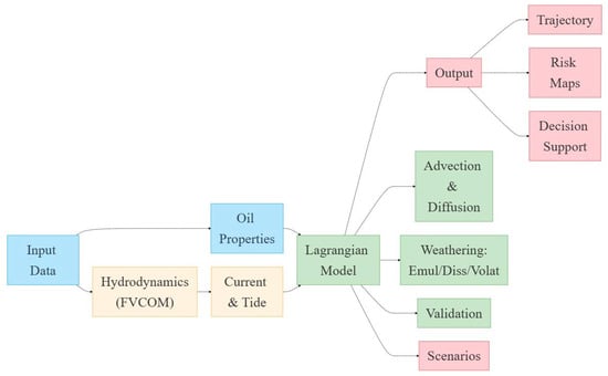
Figure 1.
The flowchart of the research framework.
2.1. Hydrodynamic Model
The FVCOM ocean hydrodynamic model is based on unstructured grids and discretized using the finite volume method [15]. Compared to structured grid models (e.g., ROMS and Delft3D), FVCOM’s triangular mesh accurately resolves the complex coastline of northwestern Hainan Island. This study employs FVCOM to establish a hydrodynamic model for the Haikou–Danzhou sea area and simulates the tidal current field. The following governing equations include the momentum equation and continuity equation [16]:
where t is time; x, y, and z represent east, north, and vertical coordinate axes, respectively; u, v, and w are velocity components in the x, y, and z directions; P is atmospheric pressure; f is the Coriolis parameter; g is gravitational acceleration; Km is the vertical rotation viscosity coefficient; and Fu and Fv represent the diffusion terms of horizontal momentum and vertical momentum.
The computational grid of the FVCOM hydrodynamic model is a triangular mesh generated using the Surface-water Modeling System (SMS 10.1) software. To enhance accuracy in the study area, the domain employs nested grids of varying resolutions, as shown in Figure 2. The coarse grid shoreline data are sourced from the National Oceanic and Atmospheric Administration (NOAA) coastline database, with bathymetry derived from NOAA’s ETOPO global terrain model. The coarse grid spans 105.663–113.542° E and 15.989–21.913° N, comprising 46,901 nodes and 91,067 triangular elements. Due to the steep bathymetric gradient in the Qiongzhou Strait, grid resolution is refined in this region. High-precision fine grid coastline data were processed using ArcGIS 10.8 software (Esri) with Landsat 8 remote sensing imagery. Fine grid bathymetry is extracted from electronic nautical charts, covering 108.923–110.881° E and 19.503–20.441° N, with 12,710 nodes and 22,903 triangular elements. The Haikou–Danzhou coastal zone, the study’s focus area, features further node densification.
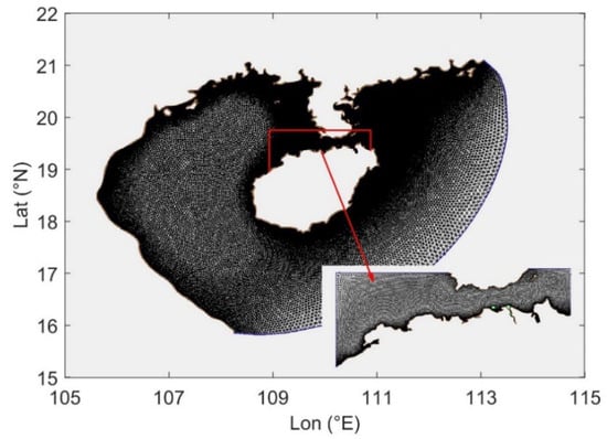
Figure 2.
Hydrodynamic model’s calculation of area size nested grid.
Tidal forcing utilizes harmonic constants for 8 principal constituents (M2, S2, N2, K2, K1, O1, P1, and Q1), 2 long-period constituents (Mf and Mm), and 3 shallow-water constituents (M4, MS4, and MN4) from Oregon State University’s TPXO global tidal model, interpolated to the coarse grid open boundary. Sea surface height and current data from the Copernicus Marine Environment Monitoring Service (CMEMS) are similarly interpolated. Tidal elevation calibration combines boundary harmonic analysis with CMEMS sea surface height. The coarse grid model employs a 20 s time step and cold-start initialization (zero initial velocity and elevation). After stabilization, coarse grid outputs (velocity and elevation) drive the fine grid through boundary interpolation. The fine grid model also uses cold-start initialization, with initial fields interpolated from the coarse grid.
The oil particle model is established based on the Lagrangian particle tracking method and random walk diffusion theory [17]. The oil film is discretized into a number of particles with Lagrangian characteristics, and the influence of random walks caused by tides, wind fields, and turbulence on the drift of oil particles on the sea surface is considered [18]. At the same time, in the process of oil particles drifting with the flow, the expansion, emulsification, dissolution, volatilization, and shore arrival processes [19] are simulated.
2.2. Oil Particle Model
In the oil particle model, uncertainties in input parameters affect prediction accuracy through coupled physical processes. Wind speed deviations directly alter surface oil film drift trajectories, with impacts modulated by the relative orientation of wind and tidal current fields. When the vector angle between these forces exceeds 45°, error propagation exhibits pronounced nonlinearity. Tidal phase uncertainty, particularly in dynamic zones like tidal fronts, is critical: temporal deviations induce advection phase shifts, causing spatial–temporal misalignment of oil film distributions. These errors are amplified during current direction reversal periods.
Among oil property parameters, the emulsification rate demonstrates the highest sensitivity. Minor variations in this rate trigger significant morphological changes in oil films via viscosity expansion positive feedback. Additionally, the temperature-dependent volatilization rate heightens prediction sensitivity to sea surface temperature data accuracy. Combined parameter uncertainties generate sublinear cumulative effects in long-term simulations and may induce phase jumps in prediction errors through oil film thickness-dependent weathering thresholds. While probabilistic ensemble forecasting and data assimilation are widely used to constrain such uncertainties, localized parameter sensitivity experiments remain essential for quantifying their impacts. Existing studies provide substantial insights into oil spill sensitivity analysis, which this work builds upon [20]. This study establishes an oil particle model based on Lagrangian particle tracking and random walk diffusion theory. The oil film is discretized into Lagrangian-representative particles, accounting for stochastic drift effects from tides, wind fields, and turbulence. During advection, the model simulates oil spill expansion, emulsification, dissolution, volatilization, and shoreline adsorption processes.
2.2.1. Expansion
According to Fay’s theory, the early stage of oil film development can be divided into three stages: the stage of gravity and inertial force, the stage of gravity and viscous force, and the stage of surface tension and viscous force [21].
where L is the equivalent diameter centered on the particle; K1, K2, and K3 are empirical coefficients, which are 2.28, 2.90, and 3.20, respectively; g is the acceleration due to gravity, which is 9.81 kg/m3; V is the volume of the oil particle; , where is the density of the oil and is the density of seawater; , where , , and are the surface tension coefficients between seawater and air, oil and air, and oil and seawater, respectively [7]; t is time; and is the kinematic viscosity of seawater.
2.2.2. Drifting
The advection process of particles is affected by tidal currents, circulation, wind fields, etc., and is the main solution of the Lagrangian particle tracking method. The advection velocity of particles is mainly controlled by the flow field and wind field and can be calculated using Equation (8) [22]:
where U and V are the flow velocities of particles in the x and y directions, respectively; Uw and Vw are the wind speeds in the x and y directions 10 m above the sea surface; Uc and Vc are the flow velocities of the ocean current in the x and y directions; and is the wind drift coefficient. According to experience, the flow velocity of wind-driven current ranges from 1% to 6% of the wind speed. In this paper, .
The Lagrangian pursuit method is mainly used to solve a nonlinear differential equation [16]:
where x is the position of the particle; v is the velocity of the particle.
The discrete integration of Equation (10) yields the following:
where tn is the time when the particle moves to xn.
The solution using the 4th-order Runge–Kutta method is as follows:
where ; ; ; ; is the time step; and xn+1 is the particle position at the next moment.
By substituting Equation (8) into Equation (11), we can obtain the position of the particle in the x and y axis directions at the next moment.
2.2.3. Diffusion
Turbulent diffusion is defined as the mass transfer caused by turbulent pulsation [23]. The turbulent diffusion process of particles is random, so the random walk method is often used to describe the turbulent diffusion process of particles to simulate the grid-scale turbulence changes in the velocity field. The turbulent diffusion of oil particles can be expressed as follows:
where Um and Vm are the turbulent diffusion velocities of particles in the x-axis and y-axis directions; R is a random number between [−1, 1]; Dx and Dy are the horizontal dispersion coefficients in the x- and y-axis directions, both of which are taken as 0.5 m/s; and is the time step of turbulent diffusion.
2.2.4. Evaporation
Evaporation is the most important mass loss process in the weathering of oil spills. In the first few days, the evaporation rate of light oil can reach 75%, and the evaporation rate of medium oil can reach 40% [24]. The evaporation rate of oil spills is calculated as follows:
where t is the time since the oil spill occurred; KE is the evaporation index, which is related to the mass migration coefficient KM: , , where A is the oil spill area; VM is the molar volume; atm-m3/(K-mol) is the gas constant; T is the oil film surface temperature; and V0 is the oil spill volume. When , the initial volatile gas pressure P0 is calculated as follows:
where T0 is the initial boiling point; TE·C is a constant. According to the calculation formula of the American Petroleum Organization,
where API is API petroleum gravity.
2.2.5. Dissolution
Although the effect of dissolution on the amount of oil during the weathering process of oil spills is relatively small and the amount of dissolution will not exceed 1% of the total oil volume, the harm caused to marine life by oil being dissolved in seawater is huge [22], so it is very necessary to calculate the dissolution process of oil spills. The calculation formula for the dissolution rate is as follows:
where K is the solubility mass transfer coefficient, calculated as , where e is determined by the properties of the oil, with values of 1.4 for alkanes, 2.2 for aromatic hydrocarbons, and 1.8 for refined oils. S is the solubility of oil in water, determined by the type of oil, calculated as follows:
where S0 is the initial solubility of oil; is the attenuation coefficient. According to the research of Lu et al. [25], the initial solubility of crude oil is 8915 mg/m2, and the attenuation coefficient is 2.38 day−1.
2.2.6. Emulsification
The emulsification of oil spills refers to the process in which oil spills gradually form stable viscous emulsions under the action of agitation on the sea surface. This emulsion will affect the evaporation and dissolution of oil spills, making the oil spills difficult to clean up [7]. Generally speaking, the emulsification process of oil spills can be characterized by the water content YW:
where KA is generally taken as ; , where is the maximum moisture content, which is 0.85 in this paper.
2.2.7. Density and Surface Tension Changes
The evaporation and emulsification processes will affect the density of the remaining oil spill. Combining the two, the final change in density can be expressed as follows [26]:
where is the initial density of the oil spill; is the density of seawater.
The formula for calculating the change in surface tension of oil is
where is the initial surface tension of the oil film; is the residual oil volume; is the emulsified oil volume.
2.2.8. Concentration
The amount of oil in each grid cell is calculated by establishing a structural grid and counting the mass of particles in each grid cell. The amount of oil per square meter is then divided by the area of the grid cell. The calculation formula is
where C is the concentration of the grid unit; Mj is the mass of the number of j particles; N is the number of particles in the grid unit; and S is the area of the grid unit.
2.2.9. Landing and Border Processing
Oil spills will run aground on the shore as they move, but due to the limited carrying capacity of the coast, part of the oil spill will return to the seawater with waves and tides. The formula for calculating the amount of oil returned to the seawater over a period of time is as follows [26]:
where is the amount of oil returned to the water; is the amount of oil reaching the shore; and is the half-life of the shoreline.
When a particle moves to the shore boundary and its position exceeds the shore boundary at the next moment, the particle position is relocated to the intersection of the motion trajectory and the shore, and the particle is considered to be stranded on the shore. Considering the carrying capacity of the coast, a shore boundary grid is set to accommodate 3 shore-reaching particles at most. When a particle crosses the free boundary, it is considered to leave the calculation domain, and its movement is no longer calculated.
2.3. Buoys and Dye Trials
To verify the reliability of the oil spill drift and diffusion model, this study conducted buoy and dye release experiments in the coastal waters from Haikou to Danzhou, simulating the drift and dispersion processes of oil spills under realistic conditions. The offshore experiments were designed according to the “worst-case conditions—typical scenarios” principle, with the trial period selected during the South China Sea’s predominant strong wind season. Historical meteorological data indicate a 63% frequency of northeast winds during this interval, averaging 6.5 m/s and generating maximum wind-driven currents of 0.28 m/s, thereby rigorously testing the model’s predictive capability under extreme conditions. The experimental sites were located within a three-nautical-mile radius of a local oil terminal, an area that had experienced seven minor oil spills over the past five years (averaging 1.4 incidents annually), reflecting its high-risk status.
The trials took place from 18 to 22 December 2024, and included two buoy drift experiments and one dye dispersion test. The first buoy trial commenced at 15:00 on December 18, deploying 15 small GPS buoys at 110.0111° E, 19.9653° N, with data being sampled every 5 min. The second buoy trial began at 15:30 on December 20, releasing 12 buoys at the same location. The dye trial started at 13:30 on December 21 at 109.9677° E, 19.9570° N, monitoring the diffusion range and center position of sodium fluorescein every 10 min for 70 min. Equipment specifications are detailed in Table 1.

Table 1.
Sea trial equipment and list of materials.
Prior to deployment, wind field conditions were measured using anemometers and cross-validated with local weather forecasts. During the trials, the first buoy experiment experienced northeast winds averaging 5 m/s, while the second buoy trial and dye test were influenced by easterly winds at 6.4 m/s and 5.2 m/s, respectively. Buoys and dye were deployed downwind from predetermined positions (as shown in Figure 3 and Figure 4). The process of the three trials is as follows:
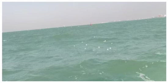
Figure 3.
Small GPS buoys dropped on the sea surface.
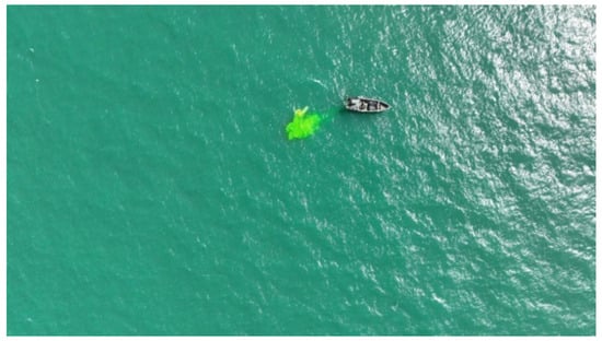
Figure 4.
Aerial photo of fluorescein sodium patch.
- (1)
- The first buoy trial: A total of 15 small GPS buoys were deployed. Under the influence of the northeast wind, the buoys moved quickly toward the shore. Two hours after deployment, all the buoys ran aground on the beach southwest of the deployment point. The grounding location of the buoys was located by the computer GPS positioning system, and the buoys were quickly recovered at the corresponding location. However, due to the large number of obstacles in the nearshore area and the damage of some buoys by local fishermen, 12 buoys were successfully recovered in the end.
- (2)
- Second buoy trial: A total of 12 small GPS buoys were deployed. Under the influence of the easterly wind, the buoys drifted along the nearshore sea surface of the coastline, maintaining good synchronization as a whole, and presenting a long strip distribution along the coast. A total of 30 h after deployment, all the buoys ran aground on the beach far west of the deployment point. After locating the grounding site through the GPS system, all the buoys were recovered.
- (3)
- Dye trial: Because sodium fluorescein has low toxicity and high biodegradability and is not likely to cause long-term environmental pollution, sodium fluorescein was used as a dye in this trial. During the trial, 200 g of sodium fluorescein was mixed with 5 L of seawater to form a uniform solution, and the solution was evenly poured into the sea surface in the downwind direction. The distribution range of sodium fluorescein on the sea surface was photographed and monitored using a drone deployed on the shore, and image data were recorded every 10 min to analyze the drift and diffusion process of sodium fluorescein. After 70 min of release, the color gradually became less obvious due to the decrease in the concentration of sodium fluorescein, and the trial ended.
2.4. Scenario Condition Setting
The sea area from Haikou to Danzhou is located in the southern part of the Qiongzhou Strait. In recent years, the Hainan COSMO terminal in Chengmai Bay has gradually been improved and put into full use. With the increase in sea oil and gas exploitation in Hainan Province, the terminal provides oil and gas supply, maintenance, and cargo loading and unloading services for more ships, resulting in increasingly busy routes in Chengmai Bay, increasing the risk of ship collision and oil spill. According to AIS data, there are many oil tankers with a load of less than 6000 DWT entering and leaving Chengmai Bay. This study selected the dense route point of Chengmai Bay (110.0116° E, 19.9622° N) as the initial point of oil spill, simulated the instantaneous leakage of 100t of medium crude oil, set 2000 oil particles, and, combined with the average seawater temperature in summer and winter, analyzed the impact of oil spill (Table 2) on five environmentally sensitive areas (ESAs) [27], which rank from 1 to 5 under different tides and wind conditions as follows: the Silverlip Pearl Oyster Marine Reserve, Huachang Bay Mangrove Marine Reserve, Shatu Bay Beach, Hainan Old Town West Coast Beach, and Dongzhai Qinglan Port Mangrove Marine Reserve (Figure 5).
Table 2.
Parameter settings of oil spill model.
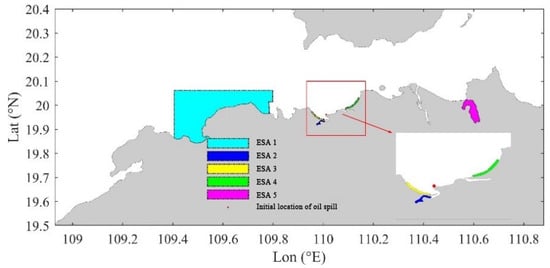
Figure 5.
Initial location of oil spill and location of environmentally sensitive areas.
Based on ECMWF ERA5 reanalysis data, the wind field characteristics of the sea area in the past 10 years are statistically analyzed (Figure 6): the dominant wind direction in summer is southerly wind (S), with an average wind speed of 3.55 m/s; the dominant wind direction in winter is northeasterly wind (NE), with an average wind speed of 4.90 m/s. According to the relative position of the oil spill point and the ESA, the most unfavorable wind direction is determined to be easterly wind (E), with a wind speed of 7 m/s. Referring to the Technical Guidelines for Environmental Risk Assessment of Oil Spills on Water [28], the simulation time is set to 72 h, and the specific working conditions are shown in Table 3.
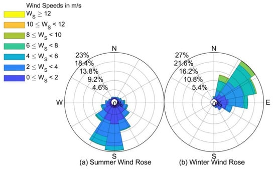
Figure 6.
Wind rose diagram of sea area from Haikou to Danzhou from 2013 to 2024.
Table 3.
Oil spill condition settings.
3. Results and Discussion
3.1. Model Validation
3.1.1. Hydrodynamic Model Validation
The accuracy of the hydrodynamic model directly determines the accuracy of the oil spill model, and the verification of the tidal field is very necessary. This paper uses the measured tidal level and flow velocity and the direction data of two tidal stations (H1 and H2) and four tidal stations (H1, H2, H3, and H4) in Haikou Bay to verify the output results of the hydrodynamic model. A high tide period is selected as the verification time (9:00 on 12 April 2019 to 10:00 on 13 April). The longitude and latitude coordinates of the tidal stations are H1: 110.2484° E, 20.0387° N, H2: 110.2579° E, 20.0703° N, H3: 110.2904° E, 20.0566° N, H4: 110.3158° E, and 20.1035° N, and the specific locations are shown in Figure 7. The verification results of the tide level are shown in Figure 8, and the verification results of the flow direction and velocity are shown in Figure 9. The hourly change trend of the simulated tide level is consistent with the actual tide level. The simulated flow field of the four tide gauges is basically consistent with the actual flow field, and the hourly change trend of the flow velocity and direction is basically consistent. In order to objectively evaluate the accuracy of the model, the correlation analysis of the simulation results and the measured results is carried out, and the Pearson correlation coefficient is used as an indicator to evaluate the effectiveness of the simulation value [29]. The calculation formula is
where R is the correlation coefficient; Xi is the number i of measured values; is the average measured value; Yi is the number i of simulated values; is the average simulated value; and n is the sample size.
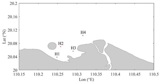
Figure 7.
Locations of tide and tidal current stations.
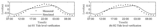
Figure 8.
Comparison and verification of measured and simulated tide levels.
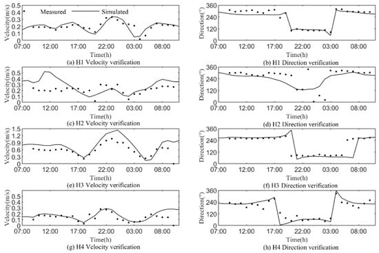
Figure 9.
Comparison and verification of measured and simulated current speeds and directions.
The correlation coefficients between the simulated values of tide level and flow direction and velocity and the measured values were calculated (Table 4). The correlations of the two tide levels are both greater than 0.96, indicating that the simulated values and the measured values are highly consistent; additionally, except for the low correlation of the velocity at the H2 tide gauge point, the tidal elements of the other stations all show a high correlation (R > 0.7). The H2 station is located near the Nanhai Pearl Artificial Island Project in Haikou Bay. The changes in the project have led to changes in the terrain and water depth nearby. There is a certain error between the terrain and water depth in the model and the terrain and water depth when the velocity was measured at that time, resulting in poor velocity simulation. However, by comparing (c) and (d) in Figure 9, it can be seen that the simulated and measured velocity and flow direction change trends at the H2 station are consistent, which can represent the real flow field to a certain extent. In addition, by adding more accurate and real terrain and water depth data, the velocity error of this point can be greatly reduced. The tidal field of the sea area at the time of rapid rise and fall is shown in Figure 10. At the time of rapid fall, the tidal current in the middle of the Qiongzhou Strait flows eastward. On the contrary, at the time of rapid rise, the tidal current in the middle of the Qiongzhou Strait flows westward. The model simulates the characteristics of water flow along the coast very well. The velocity distribution in the strait is fast in the middle and slow on both sides, which is consistent with the flow of actual ocean currents. In general, the FVCOM hydrodynamic model established in this paper can realistically simulate the flow field conditions in the sea area near Haikou to Danzhou, and the output flow field data can be used as the hydrodynamic drive of the oil spill model.
Table 4.
Tidal current element correlation coefficient (R) calculations. (Note: NA—not applicable).
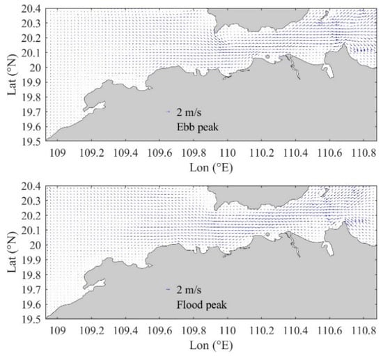
Figure 10.
Simulated current field in sea area from Haikou to Danzhou.
3.1.2. Validation of Oil Spill Drift and Diffusion Model
Figure 11 and Figure 12 show the drift and diffusion process of the oil spill sea trial and numerical simulation. The core position of the buoy group is obtained by averaging the longitude and latitude positions of the buoys with a time interval of 1 h. To assess the computational error of the numerical model, the 80% probability circle of the buoy group’s center position after grounding was calculated (the radius of the 80% probability circle is defined as 20% of the total length of the actual drift path), ensuring that the error range remains within 20%. This was determined based on the operational forecasting requirements set by management authorities [30]. Although the first buoy trial was short, the trajectory of the buoys was highly consistent with the simulation results of the oil spill numerical model. Affected by northeast wind, the buoys drifted rapidly towards the beach of Shatu Bay, arrived at the beach within 2 h, and showed the characteristics of distribution along the coastline. As can be seen from Figure 11, the simulated values of the 15 particles in the numerical model all fall within the 80% probability circle of the actual position, indicating that the simulation error rate of the oil spill drift trajectory is less than 20%. Table 5 shows the calculation results of drift simulation error in the core area of the oil spill. In the first buoy trial, the offset between the simulated value and the measured value in the core area was within 200 m. The numerical model showed high accuracy and small error, and the simulation results had strong credibility. The second buoy trial lasted for more than 24 h. The buoys always drifted along the coast and showed a long strip distribution. During this period, the buoys bypassed Shatu Bay, Qiaotou Town, and Hongshi Island, and finally ran aground on the beach of Bopu Bay. As can be seen from Figure 12, the drift paths of the trial buoys and the simulated particles are basically the same, and the simulated drift path is closer to the shore, which may be related to the difference between the nearshore terrain and water depth data in the model and the actual situation. After 24 h, the 12 particles in the numerical model all fell within the probability circle of 80% of the actual position, and the offset error was less than 20%. According to the data in Table 5, the maximum offset distance between the simulated value and the trial value in the core area in the second buoy trial is 2.24 km (<4 km), which meets the requirements of the “Inspection Specifications for Maritime Search and Rescue Forecast Products” [30] and is rated as excellent, indicating that the results of the numerical model are reliable and the error is within a reasonable range.
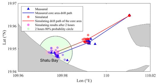
Figure 11.
The first buoy trial’s drift diffusion simulation verification.
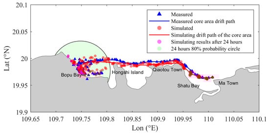
Figure 12.
The second buoy trial’s drift diffusion simulation verification.
Table 5.
Oil spill drift simulation error. (Note: NA—not applicable).
Figure 13 shows the drift and diffusion process of the dye sodium fluorescein patch in the coastal waters of Shatu Bay within 70 min. In the experiment, the patch showed a strong drift characteristic as a whole and drifted and diffused toward the shore under the influence of the easterly wind. The diffusion shape of the patch is mainly affected by the wind field [31]. The diffusion speed is faster in the downwind direction, resulting in the patch being long strips. The data in Table 6 show that the patch area continues to increase over time, reaching 6294.23 m2 after 70 min, but the area growth rate gradually decreases, indicating that the diffusion rate gradually slows down. At the same time, the drift distance growth rate of the center of the patch is relatively stable, with a total drift distance of 714.26 m and an average drift speed of 0.17 m/s, which is close to the local current speed, further verifying the drift characteristics of the sodium fluorescein patch. It can be observed from Figure 14 that the simulated oil spill area has similar diffusion laws as the area enclosed by the buoys and the dye patch area and shows consistency in overall shape. This shows that the diffusion simulation results of the oil spill model are credible and can better reflect the process of oil spill drift and diffusion in actual sea trials.
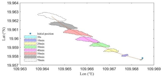
Figure 13.
Changes in the area of dye patch over time.
Table 6.
Changes in fluorescein sodium patch area and drift distance over time.
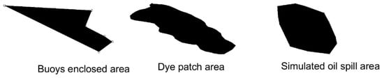
Figure 14.
Comparison of different trial and simulation results in coastal waters of Shatu Bay.
In summary, the error between the simulation results of the oil spill model and the buoy trial data is within a reasonable range, indicating that the numerical model can well restore the particle distribution and the drift trajectory of the particle group center during the buoy trial. In the dye trial, it was observed that the sodium fluorescein plaque had obvious drift characteristics with the flow, and the plaque showed a law of diffusion along the wind direction. The oil spill model successfully simulated this diffusion process and verified the feasibility of using the Lagrangian particle tracking method to numerically simulate oil spills in the waters near Haikou to Danzhou. The model results can more accurately reflect the drift and diffusion process of oil spills on the sea surface and have a high degree of credibility.
3.2. Drift and Diffusion Analysis
Through numerical simulation, the drift and diffusion behavior of oil spills under six working conditions for 72 h was studied; the distribution, movement direction, and concentration changes in oil spills were analyzed; and the swept area was calculated to determine the impact range (Figure 15). The results show that the tide dominates the movement of oil spills, showing a reciprocating drift from east to west, and the overall westward trend is obvious. The wind field has a significant impact on the spread of oil spills: in winter, northeasterly wind causes oil spills to gather on the shore, and the swept area is small, but the coastline is seriously polluted; in summer, southerly wind causes the oil spills to move northward, the diffusion range is expanded, and the swept area is the largest (995.25 km2); under the action of easterly wind, oil spills move westward, and due to terrain restrictions, the pollution of the sea area from Chengmai Bay to Yangpu is serious. The oil spill diffusion characteristics at high tide and low tide are similar, but oil spills reach the shore more easily under the action of northeasterly wind and easterly wind at high tide, resulting in aggravated coastline pollution and a decrease in subsequent oil spill concentration; under the action of southerly wind in summer, oil spills move westward around the coast, the amount reaching the shore is reduced, and the oil spill concentration remains at a high level.
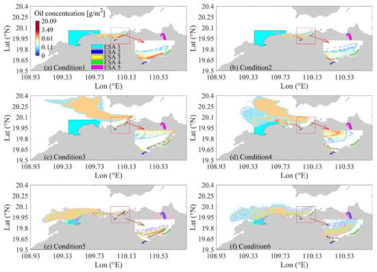
Figure 15.
Drift and diffusion distributions of oil spills under different working conditions for 72 h.
Table 7 shows that the swept area and drift track length are the largest under southerly wind conditions (995.25 km2 and 226.92 km, respectively) and the smallest under northeasterly wind conditions (106.53 km2 and 123.14 km). The low velocity area near the coast limits the spread of the oil spill, while the high velocity area in the middle of the Qiongzhou Strait accelerates the spread of the oil spill. Under the action of easterly wind, although the wind speed is high, the swept area and track length are relatively small because the path is concentrated in the low-velocity area near the coast. This study shows that the interaction between wind speed and tidal velocity significantly affects the drift behavior and distribution range of the oil spill.
Table 7.
Calculations of the sweeping area and drift track length of oil spills under different conditions.
3.3. Pollution Analysis of ESA
In order to evaluate the pollution impact of oil spills on five ESAs in the sea area from Haikou to Danzhou, we calculated the time and duration of oil spills reaching each sensitive area under six conditions (Table 8). The results show that the Lingao Silverlip Pearl Oyster Marine Reserve (ESA 1) was polluted under all conditions, among which the oil spill arrived as soon as 8 h under a rising tide and southerly wind (condition 4), the longest duration (64 h) under a rising tide and easterly wind (condition 6), and the shortest duration (3 h) under a falling tide and southerly wind (condition 3). The Huachang Bay Mangrove Marine Reserve (ESA 2) was not significantly polluted due to shoreline protection, while the Dongzhai Qinglan Port Mangrove Marine Reserve (ESA 5) was not affected because the oil spill mainly moved westward. Shatu Bay Beach (ESA 3) was polluted as soon as 2 h under a rising tide and northeasterly wind (condition 2) and lasted for 71 h; it was not polluted under southerly wind and under a falling tide and easterly wind. Hainan Old Town West Coast Beach (ESA 4) was polluted only under a low tide and northeasterly wind (condition 1), with the oil spill arriving in 6 h and lasting for 27 h.
Table 8.
Calculation of times for oil spill to affect environmentally sensitive areas. (Note: NA—not applicable).
Figure 16 shows the percentage of the cumulative pollution area of each ESA caused by oil spills under 10 pollution scenarios. The results show that ESA 3 is most seriously polluted under northeasterly wind, with a cumulative pollution area of more than 95% at high tide and about 80% at low tide, and more than 40% under easterly wind and high tide, indicating that the beach is susceptible to pollution under northeasterly wind and high tide conditions, which is manifested by a large pollution area, the early arrival of oil spills, and their long duration. The cumulative pollution area of ESA 1 is the largest under easterly wind and high tide (>70%) and >65% under easterly wind and low tide; it is the smallest under southerly wind and low tide and more than 30% under high tide and southerly wind. Under northeasterly wind, the oil spill was stranded in Shatu Bay and blocked from moving westward, and it only polluted the east side of the reserve; under southerly wind, the oil spill gradually moved away from the coast, but there was still some pollution under a high tide and southerly wind. ESA 4 was only polluted under northeasterly wind and low tide, accounting for about 15%. Under other working conditions, the oil spill was far away from the area due to the action of tide and wind field, and the area was not significantly polluted.
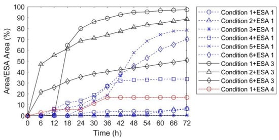
Figure 16.
Proportion of oil spill in environmentally sensitive areas.
Figure 17 shows the hourly changes in the amount of oil spilled to each ESA under different conditions. Under the influence of southerly wind and high tide conditions, the amount of oil spilled to ESA 1 reached a maximum of 67.9 tons and then rapidly decreased. This phenomenon was due to the fact that the high tide quickly transported the relatively concentrated oil spill to the reserve, and the subsequent low tide took part of the oil spill away from the reserve. Under southerly wind and low tide conditions, the amount of oil spilled in the reserve was the lowest at only 66.74 kg. For ESA 3, the maximum amount of oil spilled reached 60.7 tons. After the oil spill reached the beach, part of the oil spill remained on the beach due to the stranding effect. Due to the combined effects of the volatilization of the oil spill and the drift of part of it re-entering the seawater, the amount of oil spilled on the beach gradually decreased. The amount of oil spilled received by ESA 4 was small, with a maximum of only 103 kg, and the degree of pollution was low. This indicates that under the conditions simulated in this study, the area was relatively less affected by the oil spill.
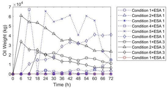
Figure 17.
Hourly changes in the amount of oil spilled in environmentally sensitive areas.
In summary, the impact of oil spills on environmentally sensitive areas under various operating conditions shows that ESA 1 was polluted to varying degrees in all operating conditions. Judging from indicators such as the arrival time, duration, the proportion of affected area, and amount of oil spilled, the most unfavorable easterly wind and high tide conditions caused the most serious pollution to the reserve, while southerly wind and low tide conditions caused the least pollution to the reserve. For ESA 3, the high tide and northeasterly wind conditions caused the highest degree of pollution to the beach, which was mainly manifested in the early arrival time of the oil spill, its long duration, and a large proportion of polluted area. ESA 4 was only polluted to a certain extent under the conditions of northeasterly wind and low tide, and the pollution level was relatively low, while no obvious pollution impact was observed under other operating conditions.
4. Conclusions
We established a hydrodynamic model through FVCOM, and on this basis, we used the Lagrangian particle tracking method to establish a numerical model of oil spill drift and diffusion. The hydrodynamic model was first verified using measured tidal data, and then the accuracy and applicability of the oil spill model were verified by combining buoy and dye trials. Finally, the established oil spill model was used to systematically study the oil spill drift and diffusion characteristics under different conditions in the sea area from Haikou to Danzhou and its impact on environmentally sensitive areas, and the following main conclusions were drawn:
- (1)
- The correlation coefficient between the simulated tidal level of the hydrodynamic model and the measured value was >0.96, and the simulated flow velocity and flow direction were highly correlated with the measured values (R > 0.7), indicating that the model can effectively characterize the tidal level and tidal dynamics of the sea area. The model accurately reproduced the characteristics of the tidal field in the study area: when the tide was falling, the tide in the middle of the Qiongzhou Strait was eastward, and when the tide was rising, it was westward, and the spatial distribution pattern of “fast in the middle and slow on both sides” was consistent with the actual observation.
- (2)
- The existing oil spill drift and dispersion studies are primarily focused on numerical models, with limited research on field experiments. This paper conducts sea buoy and dye experiments to study the drift path (macroscale) and dispersion pattern (microscale) of oil spills, validating the drift and dispersion patterns of oil spills under the influence of tidal currents and wind fields and demonstrating the applicability of the oil particle model. In the buoy trials, the drift path of the simulated particles in the numerical model was consistent with the actual buoy trajectory, with the final simulated location falling within 80% of the probability circle of the actual position, and the error was less than 20%. The root mean square error (RMSE) of the drift distance was 0.92 km, which meets the operational forecasting requirements. In the dye trial, the dispersion pattern of the fluorescein sodium patch along the coast of Shadawan was similar to the dispersion pattern of the oil spill simulation, both exhibiting characteristics of drift with the current and diffusion along the wind direction.
- (3)
- The 72 h simulation showed that the tides dominated the reciprocating drift of oil spills, and the wind field regulated the diffusion range and pollution characteristics: northeasterly wind limited diffusion but aggravated shoreline pollution (sweeping area of 106.53 km2); southerly wind drove the maximum diffusion (sweeping area of 995.25 km2; trajectory of 226.92 km); and the most unfavorable easterly wind accelerated nearshore concentrated transport, and the diffusion range was limited. The pollution risk of sensitive areas was significantly different: ESA 1 was polluted under all working conditions, and the pollution was the heaviest during easterly wind and high tide conditions (area > 70%; oil spill 67.9 tons); ESA 3 was polluted the fastest during northeasterly wind and high tide (arriving in 2 h, lasting 71 h; area 95%); and ESA 4 was only slightly polluted during northeasterly wind and low tide (area 15%; oil spill 103 kg).
- (4)
- The research results show that the numerical model of oil spill drift and diffusion based on the Lagrangian particle tracking method can accurately reflect the drift and diffusion characteristics of oil spills under different wind fields and tidal conditions, and the simulation results are highly credible. This model can be used to predict the drift trajectory of oil spills in the waters from Haikou to Danzhou, providing a scientific basis for oil spill pollution assessment and oil spill emergency prevention and control in environmentally sensitive areas.
- (5)
- The oil spill model developed in this study has successfully integrated multi-source marine ecological online monitoring data, enabling real-time data to drive the oil spill model. It has already been put into operational trial runs during emergency drills at several offshore oil and gas platforms in the South China Sea.
- (6)
- Future research will focus on advancing the coupled modeling of oil spill weathering processes and transport–diffusion dynamics. By integrating an oil weathering model, a comprehensive degradation prediction system will be developed, covering evaporation, emulsification, dispersion, photooxidation, and biodegradation. This improvement will enable a dynamic simulation of oil film residue over a 30-day period while simultaneously assessing the mortality rate of algae caused by oil film coverage.
Author Contributions
Conceptualization, W.W. and B.L.; methodology, B.L. and Z.Z.; investigation, Z.G. and W.W.; resources, B.L. and W.W.; writing—original draft, W.W.; writing—review and editing, W.W. and C.C. All authors have read and agreed to the published version of the manuscript.
Funding
This research was supported by the Hainan Province Science and Technology Project (Grand No: ZDYF2023SHFZ119).
Data Availability Statement
The data will be made available upon request.
Conflicts of Interest
The authors declare no conflicts of interest.
References
- Chen, X. Study on the Particle Tracking Based, Two-Layer Forecast Model for Oil Spills on the Sea. Dalian University of Technology. 2017. Available online: https://d.wanfangdata.com.cn/thesis/D01389054 (accessed on 22 March 2025).
- Demetrashvili, D.; Kukhalashvili, V.; Kvaratskhelia, D. Numerical study of the circulation and its contribution to the oil slick transport in the southeastern part of the Black Sea. arXiv 2023. [Google Scholar] [CrossRef]
- Wei, H.; Nian, M.; Li, L. China’s Regional Development Strategies and Policies During the 14th Five-Year Plan Period. China Ind. Econ. 2020, 5, 5–22. [Google Scholar] [CrossRef]
- Lehr, W.; Jones, R.; Evans, M.; Simecek-Beatty, D.; Overstreet, R. Revisions of the ADIOS oil spill model. Environ. Model. Softw. 2002, 17, 189–197. [Google Scholar] [CrossRef]
- Boufadel, M.; Bracco, A.; Chassignet, E.P.; Chen, S.S.; D’asaro, E.; Dewar, W.K.; Garcia-Pineda, O.; Justić, D.; Katz, J.; Kourafalou, V.H. Physical Transport Processes that Affect the Distribution of Oil in the Gulf of Mexico. Oceanography 2021, 34, 58–75. [Google Scholar] [CrossRef]
- Mackay, D. Oil Spill Processes and Models; Environmental Impact Control Directorate, 1980. Available online: https://search.worldcat.org/zh-cn/title/1240697685 (accessed on 22 March 2025).
- Zhen, Z. Research of Offshore Oil Spill Numerical Modeling and Application to Luanjiakou Port Area in Bohai Bay. Master’s Thesis, Tianjin University, Tianjin, China, 2017. [Google Scholar]
- Kistovich, A.; Chaplina, T. Analytical and experimental modeling of the hydrocarbon slick form and its spreading on the water surface. Phys. Fluids 2021, 33, 076605. [Google Scholar] [CrossRef]
- Qiao, J.; Song, Y.; Xia, H.; Zhang, L. Research on Comparison of FAY Model and Oil Particle Model for Oil Spill Simulation in River–Channel Reservoirs. Yangtze River 2019, 50, 29–33. [Google Scholar]
- Yang, H.; Liu, C.; Li, Y.; Ding, L. Numerical simulation of oil-spill in the south channel of the stuary Yangtze River estuary. Mar. Sci. Bull. 2013, 32, 345–351. [Google Scholar]
- Sakar, C.; Toz, A.C.; Koseoglu, B. Numerical modelling of oil spill in New York Bay. Arch. Environ. Prot. 2016, 42, 22–31. [Google Scholar]
- Sun, Y.; Liu, D.; Xu, Y.; Li, Z.; Han, Z. Numerical Simulation of Oil Spilling Drift and Diffusion in Zhanjiang Bay. Trans. Oceanol. Limnol. 2022, 30, 73–83. [Google Scholar]
- Zhao, X.; Wang, X.; Wu, L.; Xing, C.; Huo, R. The Oil Spill Risk Simulation in Weitou Bay and Its Impact on the Surrounding Environmentally Sensitive Area. Mar. Forecast. 2023, 40, 57–64. [Google Scholar]
- Guo, Z.; Xiao, J.; Liu, J.; Hu, X. Comparison of structured and unstructured grids in marine controlled source electromagnetic inversions for offshore hydrocarbon exploration. Mar. Pet. Geol. 2019, 100, 204–211. [Google Scholar] [CrossRef]
- Yang, Z.; Shao, W.; Hu, Y.; Ji, Q.; Li, H.; Zhou, W. Revisit of a case study of spilled oil slicks caused by the Sanchi accident (2018) in the East China Sea. J. Mar. Sci. Eng. 2021, 9, 279. [Google Scholar] [CrossRef]
- Chen, C.; Beardsley, R.C.; Cowles, G. An Unstructured Grid, Finite-Volume Community Ocean Model: FVCOM User Manual; Sea Grant College Program, Massachusetts Institute of Technology: Cambridge, MA, USA, 2011. [Google Scholar]
- Dąbrowska, E. Numerical Modelling and Prediction of Oil Slick Dispersion and Horizontal Movement at Bornholm Basin in Baltic Sea. Water 2024, 16, 1088. [Google Scholar] [CrossRef]
- Van Dang, H.; Joo, S.; Lim, J.; Hur, J.; Shin, S. Numerical Model Test of Spilled Oil Transport Near the Korean Coasts Using Various Input Parametric Models. J. Ocean. Eng. Technol. 2024, 38, 64–73. [Google Scholar] [CrossRef]
- Eke, C.D.; Anifowose, B.; Van De Wiel, M.J.; Lawler, D.; Knaapen, M.A. Numerical modelling of oil spill transport in tide-dominated estuaries: A case study of Humber Estuary, UK. J. Mar. Sci. Eng. 2021, 9, 1034. [Google Scholar] [CrossRef]
- Roman, F.; De Leo, F.; Cavallaro, L. Numerical Monitoring of Oil Spill Scenarios in Augusta Harbour. In Proceedings of the 2023 IEEE International Workshop on Metrology for the Sea, Learning to Measure Sea Health Parameters (MetroSea). La Valletta, Malta, 4–6 October 2023; pp. 369–373. [Google Scholar]
- Fay, J.A. The spread of oil slicks on a calm sea. In Proceedings of the Oil on the Sea: Proceedings of a Symposium on the Scientific and Engineering Aspects of Oil Pollution of the Sea, Cambridge, MA, USA, 16 May 1969; pp. 53–63. [Google Scholar]
- Shen, H.T.; Yapa, P.D. Oil slick transport in rivers. J. Hydraul. Eng. 1988, 114, 529–543. [Google Scholar] [CrossRef]
- Zhang, Z.; Cui, G. Fluid Mechanics; Tsinghua University Press Co., Ltd.: Beijing, China, 1999; Available online: https://www.tup.com.cn/booksCenter/bookcatalog.html?id=01681408 (accessed on 22 March 2025).
- Betancourt, F.; Palacio, A.; Rodriguez, A. Effects of the mass transfer process in oil spill. Am. J. Appl. Sci. 2005, 2, 939–946. [Google Scholar]
- Lu, B.C.Y.; Polak, J. Study of the Solubility of Oil in Water: Report; Environment Canada, Environmental Protection Service, Environmental Conservation Directorate: Ottawa, ON, Canada, 1973; Available online: https://search.worldcat.org/zh-cn/title/9528623 (accessed on 22 March 2025).
- Wang, S.; Shen, Y.; Zheng, Y. A Two-Layer Mathematical Model for Oil Spill Transportand Transformation in the Sea. Chin. J. Theor. Appl. Mech. 2006, 38, 452–461. [Google Scholar]
- Huang, W.; Zeng, J.; Chen, Q.; Du, P.; Tang, Y.; Yang, H. Preliminary research on the zoning method of the marine ecological red line: Acase study of Hainan Province. Acta Ecol. Sin. 2016, 36, 268–276. [Google Scholar]
- JT/T 1143-2017, 17; Technical Guidelines for Environmental Risk Assessment of Oil Spills on Water. Ministry of Transport of the People’s Republic of China: Beijing, China, 2017. Available online: https://std.samr.gov.cn/hb/search/stdHBDetailed?id=8B1827F24534BB19E05397BE0A0AB44A (accessed on 22 March 2025). (In Chinese)
- Xu, W. A Review of Correlation Coefficient Research. J. Guangdong Univ. Technol. 2012, 29, 12–17. [Google Scholar]
- HY/T 0389-2023, 10; Inspection Specification for Maritime Search and Rescue Forecast Products. NMEFC: Beijing, China, 2023. Available online: https://ndls.org.cn/standard/detail/fff19f55f2a7e17badc673bc0cd68f51 (accessed on 22 March 2025). (In Chinese)
- Blair, D.; Zheng, Y.; Bourassa, M.A. The effect of surface oil on ocean wind stress. Earth 2023, 4, 345–364. [Google Scholar] [CrossRef]
Disclaimer/Publisher’s Note: The statements, opinions and data contained in all publications are solely those of the individual author(s) and contributor(s) and not of MDPI and/or the editor(s). MDPI and/or the editor(s) disclaim responsibility for any injury to people or property resulting from any ideas, methods, instructions or products referred to in the content. |
© 2025 by the authors. Licensee MDPI, Basel, Switzerland. This article is an open access article distributed under the terms and conditions of the Creative Commons Attribution (CC BY) license (https://creativecommons.org/licenses/by/4.0/).