Optimizing Filter Element Seepage Well Layouts for Urban Flood Mitigation: A Multi-Objective Genetic Algorithm Approach

Abstract

The rapid acceleration of urbanization, combined with the proliferation of impervious surfaces and the inherently low permeability of soil layers, has worsened urban waterlogging. This study explores the layout of filter element seepage wells within a sponge city framework to enhance rainwater infiltration and reduce surface water accumulation, proposing an optimized method for determining well spacing and depth. The optimization uses a multi-objective genetic algorithm to target the construction cost, seepage velocity, total head, and pore water pressure. A combined weighting method assigns weights to each aim, while the Technique for Order Preference by Similarity to an Ideal Solution (TOPSIS) determines the perfect spacing and depth. The results show that the optimal spacing and depth of the filter element seepage wells are 1.572 m and 2.794 m, respectively. Compared to the initial plan, the optimized scheme reduces construction costs by 21.31%, increases the rainwater infiltration efficiency by approximately 200%, raises the total hydraulic head by 17.23%, and decreases the pore water pressure by 5.73%. Sensitivity analysis shows that the optimized scheme remains stable across different weight combinations. This optimized layout significantly improves both the infiltration capacity and cost-effectiveness.

1. Introduction

In recent years, urbanization and climate warming in China have accelerated, leading to increased road hardening [1,2,3,4], reduced permeable pavement areas, and a significant rise in urban flooding risks, including frequent flooding during rainfall events [5,6]. To tackle challenges in water ecology, security, and the environment [7], China has actively promoted sponge city construction since 2013 [8,9,10].

Implementing drainage measures such as rain gardens, swales, green roofs, ecological porous fiber cotton modules, and filter element seepage wells can transform cities into “sponge bodies” that naturally accumulate, infiltrate [11], and purify water [12,13,14,15,16,17], enhancing resilience to natural disasters. Among these measures, filter element seepage well technology stands out as an underground reservoir system that uses existing strata for water storage. Embedding perpendicular permeable concrete filter cores in soil layers allows it to quickly direct rainwater into deeper soil, effectively mitigating urban flooding.

Filter element seepage wells are essential for mitigating urban flooding by enhancing surface water infiltration, reducing runoff, and replenishing groundwater resources. Numerous studies have examined the infiltration efficiency of these wells. For instance, Cheng Xuelei et al. found through in situ experiments that filter element seepage wells significantly improve the efficiency of rainwater infiltration and soil saturation [18]. Zhu Xi et al. demonstrated that using construction waste as a filling material improves water permeability and enhances the infiltration efficiency [19]. Feng Yanfang et al. found that filling infiltration wells with medium and coarse sand significantly boosts the rainwater infiltration efficiency [20]. Liu Yexuan et al. proposed a vertical infiltration well device filled with coarse aggregates such as sand and gravel, demonstrating superior water permeability [21].

Despite extensive research on filter element seepage wells’ components, the influence of layout spacing and depth on rainwater infiltration has received less attention. However, these factors are crucial for optimizing infiltration performance.

This study explores the layout of filter element seepage wells in urban areas to enhance rainwater infiltration and reduce urban flooding risks. Specifically, the research will evaluate the effects of the well layout spacing and depth on infiltration efficiency using a multi-objective genetic algorithm. The study will assess different configurations regarding the construction cost, seepage velocity, total head, and pore water pressure.

Additionally, sensitivity analysis will examine the stability of the optimal solution across varying weight combinations, providing valuable insights for the effective design of sponge city drainage systems. The entropy of weight method, analytic hierarchy technique (AHP), and TOPSIS will be used to evaluate the optimal solutions, ensuring that the findings offer an effective approach to the rational layout of filter element seepage wells in sponge city projects.

2. Filter Element Seepage Well Technology

Filter element seepage wells are a cost-effective infiltration system for sponge cities. They reduce surface runoff, accelerate rainwater infiltration, and quickly channel rainwater into deep soil [21].

Infiltration Characteristics and Performance of Filter Element Seepage Wells

Due to their high permeability coefficient, which significantly exceeds that of the surrounding soil, filter element seepage wells enhance rainwater infiltration and the runoff reduction efficiency, effectively mitigating waterlogging risks [22]. Figure 1 illustrates the seepage effect and physical structure.

3. Overview of the Research Area and Model Construction

This chapter offers a comprehensive overview of the research area and develops a numerical model based on field measurements, followed by an in-depth analysis of the region’s seepage performance.

3.1. Research Area Overview

The research area is located within a research institute in Tianjin and covers approximately 360 square meters. This region experiences a typical warm temperate semi-humid monsoon climate with defined seasons. The mean annual temperature ranges from 12 to 15 °C, with rainfall primarily concentrated in July and August. The average annual precipitation is 600–700 mm, over 60% of which occurs during summer. Due to the dense surrounding buildings and limited permeable pavement, the existing drainage system has inadequate design capacity. This results in difficulties with timely surface water drainage during heavy rains and weak rainwater infiltration, failing to replenish groundwater resources effectively. The topography in this region is predominantly level with slight variations, which allows for even water distribution and reduces the impact of topographic variations. This topographic characteristic provides favorable conditions for the layout of seepage wells, facilitating the optimization and implementation of the filter element seepage well scheme. The red dotted line in Figure 2 demarcates the perimeters of this study region.

3.2. Model Development

A numerical simulation utilizing the MIDAS model was performed to evaluate the seepage efficacy of the filter wells in the research region. The MIDAS model is a well-established hydrological and hydraulic tool for modelling the groundwater flow, infiltration, and pore water pressure. It is particularly effective at simulating water flow in low-permeability soil layers and assessing the impact of well placement on precipitation infiltration.

3.2.1. Model Parameters

Based on field sampling results, the soil stratigraphy in the study area consists, from top to bottom, of a 1 m thick unreinforced fill layer, a 2 m thick clay layer, and an underlying layer of mucky soil. The building area is modelled as an impermeable layer with a thickness of 50 cm to simulate its lack of permeability. The permeable pavement area, consisting of a 50 cm thick sidewalk, has filter core seepage wells installed beneath it. The road surface area is considered a weakly permeable layer consisting of the surface, base, and cushion layers. The physical parameters for the model were selected based on measured data from typical soil layer structures in Tianjin and relevant literature [22,23]. The parameters from the literature were primarily used as supplementary reference values, and all core analysis results are based on the actual field data obtained in this study. Specific dates are included in

Table 1. Physical parameters of soil and paving materials.

Soil Layer Properties	Depth (m)	Initial Void Ratio	Saturated Unit Weight (kN/m3)	Permeability Coefficient (m/s)
Plain Fill	1	0.81	21	8.0 × 10−6
Clay	2	0.51	21	1.2 × 10−6
Mucky Soil	2	0.55	21	8.5 × 10−7
Filter Element Seepage Well	1–3	0.5	25	1.0 × 10−2
Permeable Pavement	0.5	0.6	28	2.0 × 10−2

and

Table 2. Pavement structural characteristics and parameters.

Physical Parameters	Upper Layer	Middle Layer	Lower Layer	Upper Base Layer	Lower Base Layer	Sub-Base Layer
Thickness (m)	0.04	0.06	0.08	0.12	0.32	0.18
Elastic Modulus (Mpa)	1148	984	820	500	1500	750
Permeability Coefficient (×10−8 m/s)	213	107	107	3000	3000	3000

and Figure 3.

3.2.2. Design of Rainfall Intensity

The layout of the filter element seepage wells should align with a suitable rainfall intensity design to optimize infiltration under varying rainfall conditions. This study uses the storm intensity formula from the “Standard for Calculation of Rainwater Runoff in Tianjin” for the rainfall design [24]. The study area falls within Storm Intensity Zone I, and the corresponding storm intensity formula is as follows:

$$\mathit{q}={\displaystyle \frac{2141(1+0.7562\lg \mathit{P})}{{(\mathit{t}+9.6093)}^{0.6893}}}$$

(1)

In the formula, q denotes the design rainfall intensity (L/s·ha), P is the recurrence period of the design rainfall (a), and t is the total rainfall duration (min).

Using recent rainfall data from Tianjin and accounting for the area’s rainfall characteristics and extreme weather conditions, the simulated rainfall duration is set at 120 min, with a recurrence period of 50 years.

3.2.3. Simulation of the Proposed Scheme

The number and placement of filter element seepage wells must be carefully planned based on the topography and soil permeability of the study area to optimize the drainage efficiency. Due to this region’s stringent protection and drainage requirements, a rectangular layout was selected, with seepage wells placed around the building’s perimeter. This layout ensures comprehensive coverage, facilitates uniform rainwater infiltration, and minimizes the adverse effects of water accumulation. The numerical model employs a hybrid mesh generation method to discretize a 20 m × 16 m domain. The model contains 489,495 nodes and 1,116,201 elements. Detailed layout plans and the numerical model are shown in Figure 4 and

Table 3. Design of layout configuration.

Scheme	Groundwater Level (m)	Rainfall Intensity (mm/min)	Diameter of the Seepage Well	Spacing Between Filter Element Seepage Wells (m)	Depth of Filter Element Seepage Wells (m)
Scheme 1	4	1.027	0.1	1	1
Scheme 2				1	2
Scheme 3				1	3
Scheme 4				2	3
Scheme 5				3	3

.

In the infiltration analysis, the Mohr–Cullen model is used to simulate the constitutive behavior of the soil. The unsaturated soil characteristics are accounted for using the unsaturated soil characteristic function, with the Gardner coefficient chosen as its functional form [25]. The initial water head is set 4 m below the road surface. The infiltration process consists of two stages: an initial steady-state phase that reflects the initial water head, followed by a transient phase lasting 120 min, subdivided into 10 time steps, each 10 min long.

3.2.4. Analysis of Effects

This study utilized observation data from a point 1 m beneath the ground surface to evaluate the influence of the filter element seepage well on the seepage velocity, pore water pressure, and total head across various depth and spacing combinations. It also explored how different schemes affected the effectiveness of addressing water accumulation issues in the area. Specifically, Schemes 1, 2, and 3 have the same spacing but different depths, while Schemes 3, 4, and 5 have the same depth but varying spacings. To facilitate comparison, the analysis diagrams for seepage velocity, pore water pressure, and total head include legends labelled “Scheme” to distinguish between the configurations.

Seepage velocity refers to the rate at which water flows through soil or rock and is typically used to characterize the water flow rate in porous media. Pore water pressure refers to the pressure applied by water within the voids of soil, influencing the permeability and mechanical properties of the soil. Total head is the total energy of a fluid at a given point, comprising the pressure head, elevation head, and kinetic head. In hydrological analysis, the total head is commonly used to describe the state of groundwater flow [23].

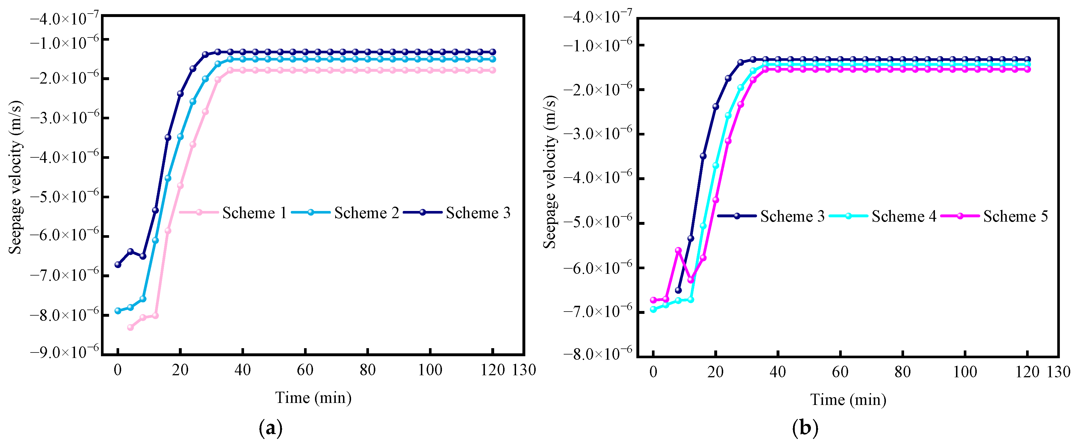
(1) Analysis of the Seepage Velocity

As shown in Figure 5a, the depth of filter element seepage wells significantly influences the seepage velocity of the soil layer. During the first 20 min of rainwater infiltration, the seepage velocity fluctuates slightly before rapidly increasing. The soil layer near the 3 m deep filter element seepage well reaches a peak seepage velocity of −1.322 × 10⁻⁶ m/s earlier. The seepage velocity of the surrounding soil is 31.6% and 18.8% faster than that of the 1 m and 2 m depth filter core wells, respectively. This increase may be due to a higher pore water pressure, which promotes faster infiltration, and the larger water storage space, which increases the seepage velocity. After 40 min, the seepage velocities at all depths stabilize.

Figure 5b illustrates the effect of the unequal spacing of filter wells on the seepage velocity within the soil layer. The filter element seepage well with a 1 m interval reaches a stable seepage velocity of −1.322 × 10⁻⁶ m/s earlier than the 2 m and 3 m interval wells. Its seepage velocity is 14.70% and 20.80% higher, respectively. This is because a smaller interval allows water to converge to the seepage well more quickly, thus accelerating the initial infiltration rate. In contrast, the filter element seepage wells with 2 m and 3 m intervals exhibit slower increases in the seepage velocity, as water takes longer to converge within the soil layer. This suggests that smaller interval arrangements are more effective at accelerating rainwater infiltration in the short term.

(2) Analysis of Pore Water Pressure

Figure 6a illustrates the effect of infiltration wells with filter cores of varying depths on the pore water pressure in soil layers. As the rainfall duration increases, the pore water pressure rises at all depths, with the most significant increase occurring within the first 20 min. The increase in pore water pressure slows and stabilizes at 18.650 kN/m². At a depth of 3 m, the pore water pressure is 13.37% and 6.28% higher than at 1 m and 2 m, respectively. This occurs because, as the soil saturates, the rainwater infiltration rate decreases, and pore water pressure results from the interaction between soil particles and pore spaces. A slower seepage velocity reduces the pressure that water exerts on soil particles or pores, reducing the pore water pressure.

Figure 6b illustrates the effect of filter wells with unequal spacing on the pore water pressure within the soil layer. The pore water pressure in the 1 m spaced filter core is much higher than in the 2 m and 3 m cores, reaching 18.650 kN/m², and is 4.83% and 11.54% higher, respectively. This is likely due to the longer infiltration and diffusion paths in filter cores with larger spacings, which slow rainwater infiltration and result in a lower pore water pressure.

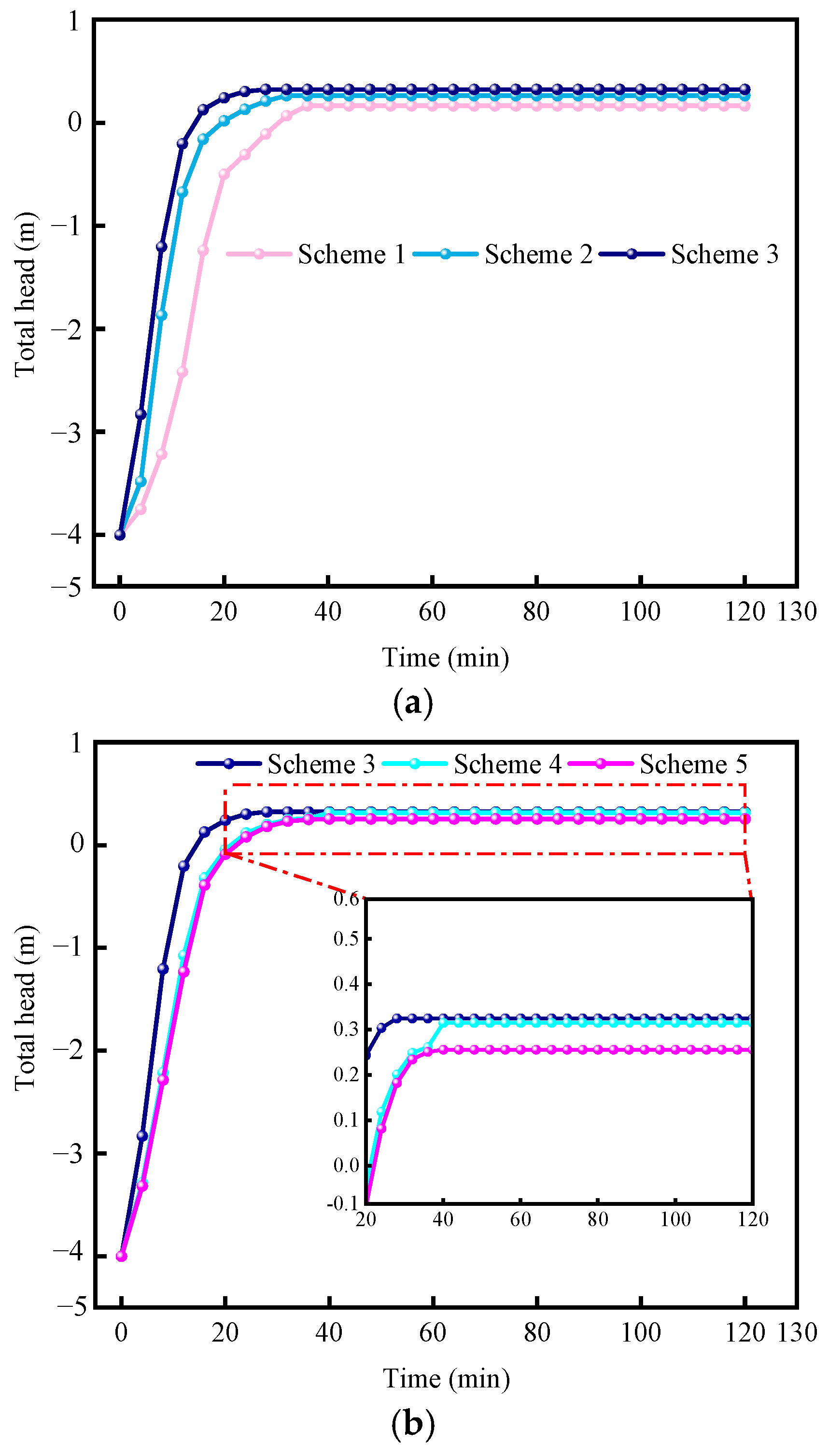
(3) Analysis of the Total Head

Figure 7a illustrates the effect of the filter well depth on the total head. Over time, the total head increases gradually, with a particularly rapid rise at the onset of rainfall. The 3 m deep filter well exhibits the fastest total head growth, stabilizing first at 0.325 m, 95.78% and 22.64% higher than the 1 m deep and 2 m deep filter wells, respectively. This suggests that deeper filter wells have a greater rainwater collection capacity. The longer infiltration path allows water to spread and accumulate more easily downward, accelerating the total head increase rate.

Figure 7b illustrates the effect of filter well spacing on total head. Although the filter well depth is constant, increasing the spacing slows the growth rate of the total head. The total head stabilizes at 0.371 m for the 1 m spacing, which is 15.56% and 26.95% higher than the total head at 2 m and 3 m spacings, respectively. This is likely due to the larger spacing, which causes water flow to spread over a wider soil area, increasing the distance to the filter well. This results in slower water accumulation around the well and a reduced increase in total head.

These simulation results highlight the fundamental relationships between the well spacing, depth, and seepage performance, which will inform the construction of the objective functions for optimization in Section 5.

(4) Differences in the effectiveness of water accumulation improvement across different schemes.

Under a rainfall intensity of 1.027 mm/min for 120 min, the simulation results indicate that the initial surface flow in this area is 29.5776 m³, with surface water accumulation at 0.1 m. A simulation analysis of the impact of varying filter element seepage well arrangements (depth and spacing) on surface flow and water accumulation (see Figure 8) reveals that the scheme with a 1 m spacing and 3 m depth is the most effective. After the seepage velocity, pore water pressure, and other factors stabilize, the surface flow of this scheme is 15.975 m³, with surface water accumulation at 0.05325 m. These values represent a reduction of approximately 45.99% in surface flow and 46.75% in water accumulation compared to initial conditions. At a constant spacing, the surface flow and water accumulation at a depth of 3 m are reduced by 22.45% and 20.89%, respectively, compared to depths of 1 m and 2 m. At a constant depth, the surface flow and water accumulation with a 1 m spacing are reduced by 18.30% and 18.98%, respectively, compared to spacings of 2 m and 3 m.

Numerical simulations were conducted to analyze the seepage effects of filter element seepage wells under various spacing and depth combinations. The results indicate that the spacing and depth strongly influence the seepage velocity, pore water pressure, and total head of filter element seepage wells. A smaller spacing and deeper well arrangement significantly enhance seepage efficiency in the initial stage, reducing surface flow and water accumulation. In contrast, a larger spacing and shallower depth result in a slower response.

3.2.5. Model Validation

(1) On-site experimental verification

Field experiments were conducted in the research area described in Section 3.1 to validate the reliability of the numerical model. Considering the need for test operability and efficient data collection, a 9 m × 5 m area adjacent to the research institute was selected as the experimental site. The precision and reliability of the numerical model were further validated by juxtaposing the simulation results with the empirical data from the field experiments.

(2) Experimental setup

The experimental setup and its on-site arrangement are shown in Figure 9. The test apparatus includes a rainfall simulation system, a data acquisition system, a power supply, a pore pressure gauge, water storage tanks, and additional components. The rainfall simulation system uses a support frame, water delivery hoses, and nozzles to replicate natural rainfall conditions, ensuring the experimental results’ uniformity and reliability. The support frame is constructed from square steel bars, each 1 m long and 2 cm wide. Baffles are installed around the frame to prevent water overflow, and gaps between the frame and the ground are sealed with adhesive material to improve sealing and reduce boundary effects.

(3) Experimental protocol

Five filter well arrangement schemes, derived from numerical simulations, were evaluated through field experiments. The experimental conditions replicated those of the numerical simulations, with a rainfall intensity of 1.027 mm/min, corresponding to a 50-year return period storm, and 120 min. The soil layer parameters are provided in Table 1. Due to spatial constraints at the test site, the experiments were conducted in sequential batches, with one arrangement scheme implemented per batch to ensure data independence. Detailed experimental schemes are outlined in

Table 4. Experimental protocol.

Scheme	Spacing Arrangement (m)	Depth of Placement (m)	Assignment Count (Items)
Scheme 1	1	1	16
Scheme 2	1	2	16
Scheme 3	1	3	16
Scheme 4	2	3	8
Scheme 5	3	3	4

.

(4) Experimental methods

The experiment was conducted five times, with a pore pressure gauge placed at a depth of 1 m in the center of each filter-element seepage well to monitor variations in the pore water pressure. Figure 10 shows the layout diagram, illustrating the spacing arrangement of the filter-element seepage wells, with the depth configuration increased accordingly.

First, the filter-element seepage wells were installed at the specified intervals and depths for each scheme, with the pore pressure gauges positioned concurrently. The rainfall simulation device was then set up in the test area. The rainfall simulation test began after connecting the data acquisition system, continuously monitoring pore water pressure variations. Finally, the collected experimental data were processed and compared with the simulated data for comprehensive analysis.

(5) Comparison of simulation results and experimental data

Pore water pressure is a key dynamic indicator for evaluating the seepage performance of filter element seepage wells, directly affecting the rainwater infiltration efficiency and soil stability. Pore water pressure data from field tests are intuitive and accessible but constrained by on-site conditions. Therefore, the model’s accuracy is primarily evaluated by comparing the pore water pressure during validation.

Figure 11a illustrates that the simulated and measured pore water pressures gradually increase with an increasing rainfall duration at varying depths, exhibiting highly consistent trends. Figure 11b shows that with varying spacings, both the simulated and measured pore water pressures increase over time, following consistent trends. While there are some discrepancies between the simulated and measured pore water pressures in Figure 11, the average error in Figure 11a is approximately 7%, with a maximum error of about 13%. In Figure 11b, the average error is around 7%, with a maximum error of approximately 16%. However, the simulation and measurement generally follow the same trend. These errors arise partly due to the influence of surrounding environmental factors and partly from the precision of the measurement equipment and the non-uniformity of the soil. Overall, the simulation results align well with the measured data, confirming the reliability of this numerical model.

(6) Validation of literature

The simulation results indicate that key indicators, such as the pore water pressure, seepage velocity, and total head, align with the existing literature. The model demonstrates that smaller spacing and the deeper placement of infiltration wells significantly improve the seepage efficiency in the initial stage, reducing surface runoff and water accumulation. In contrast, larger spacing and shallower depths lead to slower response times. These findings are consistent with reference [23], which states that “Deeper filter element seepage wells improve vertical infiltration, while smaller spacings enhance horizontal infiltration”. Furthermore, the results corroborate with reference [25], which indicates that “As rainfall duration increases, pore water pressure, total head, and seepage velocity stabilize after 120 min”.

Based on the validated model, this study used an initial scheme with a spacing of 1 m and a depth of 3 m. Under the designed rainfall condition of 120 min, this scheme exhibited the following characteristics: a seepage velocity of −1.322 × 10⁻⁶ m/s (Figure 5a), a pore water pressure of 18.718 kN/m² (Figure 6a), and a total head of 0.325 m (Figure 7a). A multi-scheme comparative analysis (Table 3) revealed significant advantages in seepage efficiency and other aspects, leading to its selection as the initial scheme for subsequent optimization studies.

This study provides essential initial conditions and design guidelines for optimizing filter well arrangements. Further research will identify the most effective depth and spacing configurations, particularly for extreme rainfall events, to ensure scientific accuracy and engineering feasibility in the final design.

4. Optimization of Filter Element Seepage Well Spacing and Depth

Building on the numerical simulation from the previous section, the impact of various depth and spacing combinations on the percolation effect of filter element seepage wells was examined. This section employs a genetic algorithm to optimize the layout of filter element seepage wells, aiming to achieve the optimal percolation effect based on these parameters.

4.1. Genetic Algorithm

This study utilizes a multi-objective genetic algorithm grounded in the Non-dominated Sorting Genetic Algorithm II (NSGA-II) for optimization [26,27]. The NSGA-II algorithm performs exceptionally well in solving nonlinear and multi-objective optimization problems. By simultaneously addressing the non-dominated relationships among multiple objectives, NSGA-II effectively overcomes the limitations of traditional optimization methods, particularly when faced with complex boundary conditions or limited data. Specifically, NSGA-II combines non-dominated sorting with a crowding distance calculation mechanism, evolving through genetic operations such as crossover and mutation. This process converges to the Pareto front, producing optimal candidate solutions. The optimization process is illustrated in Figure 12.

4.2. Objectives and Constraints of the Optimization Process

Multi-objective optimization theory suggests that independently setting objectives preserves each indicator’s characteristics and offers greater weight distribution flexibility. This approach avoids merging objectives into a single metric, which may degrade the performance of certain indicators [28], thus ensuring the scientific validity and applicability of the schemes.

This study aims to optimize the spacing and depth of filter element seepage wells to maximize the infiltration efficiency and mitigate water accumulation under rainfall conditions.

The optimization objectives comprehensively consider the seepage velocity, total head, and pore water pressure while also controlling the construction cost of the filter core infiltration wells to ensure economic feasibility and optimal performance at a low cost. These objectives encompass the key performance indicators of filter element seepage wells, including economic factors and the infiltration efficiency, with independent physical significance and practical engineering value.

Additionally, various constraints are considered to ensure the practicality and feasibility of the final scheme.

4.2.1. Objective Function

(1) The total cost of installing the filter element seepage well consists primarily of material, drilling, machine relocation, labor, and other related expenses. The labor cost is 150 RMB per day, with a construction period of 4 days, requiring three workers daily. The total labor cost for the entire project amounts to 1800 RMB. The material cost for the filter element seepage well is 5 RMB per meter, the drilling cost is 100 RMB per meter, and the machine relocation cost is 80 RMB per meter. The total cost Z of installing the filter element seepage well in the study area is

$$\mathit{Z}=5\mathit{x}+100\mathit{x}+(27{\mathit{y}}^2-143\mathit{y}+200)80\mathit{y}+1800$$

(2)

In the formula, x represents the depth of each filter element seepage well (m) and y represents the distance between two adjacent wells (m). The terms 5x and 100x represent the costs associated with the depth (RMB). The expression 27y² − 143y + 200 represents the number of filter element seepage wells, with a goodness of fit R² = 1, and is dimensionless. Finally, Z denotes the total cost (RMB).

(2) By analyzing the variation in the total head during the seepage process and using the goodness of fit R² = 0.980, the fitting results are presented in Figure 13a. The corresponding objective function is as follows:

$$\mathit{H}=0.097\mathit{x}-0.051\mathit{y}+0.122$$

(3)

In the formula, 0.097 represents the change in head per meter of depth variation along the x-direction (dimensionless). In contrast, −0.051 represents the change in head per meter of distance variation along the y-direction (dimensionless). In addition, 0.122 is the initial reference value of the head (m), and H denotes the total head (m).

(3) Seepage velocity is closely related to the spacing and depth of the filter element seepage wells, which influence the seepage efficiency. Based on the goodness of fit R² = 0.968, the fitting results are presented in Figure 13b. The corresponding objective function is as follows:

$$\mathit{L}=2.998\cdot {10}^{-7}\mathit{x}-1.944\cdot {10}^{-7}\mathit{y}-1.92\cdot {10}^{-6}$$

(4)

In the formula, 2.998 × 10⁻⁷ represents the depth influence coefficient (s⁻¹), −1.944 × 10⁻⁷ is the spacing influence coefficient (s⁻¹), and −1.92 × 10⁻⁶ is the initial seepage velocity (m/s). L denotes the seepage velocity (m/s).

(4) Pore water pressure is used as the objective function. Based on the goodness of fit R² = 0.923, the fitting result is presented in Figure 13c. The corresponding objective function is as follows:

$$\mathit{K}=1.07\mathit{x}-0.902\mathit{y}+16.323$$

(5)

In the formula, 1.07 represents the depth pressure gradient (kN/m³), −0.902 is the spacing pressure gradient (kN/m³), and 16.323 is the initial pore water pressure (kN/m²). K denotes the pore water pressure (kN/m²).

4.2.2. Constraints

The constraints and boundaries of the design variables in this study were determined based on the soil characteristics and permeability of the research area. Specifically, the depth of the filter element seepage well was set between 0 and 3 m to ensure effective infiltration and prevent soil instability due to excessive depth. The spacing of the filter element seepage wells was set between 0 and 3 m, considering the soil permeability and construction feasibility. Given the diversity of engineering practices, these constraints incorporated common engineering practices and regional characteristics, ensuring that the optimization model’s results are practical and operable. The specific constraint conditions are presented in Formula (6).

$$0<x<3, 0<y<3$$

(6)

4.3. Determination of Indicator Weights

Indicator weights are critical for evaluating the effectiveness of filter well arrangements. Common methods for determining indicator weights include subjective, objective, and combined weighting methods [29]. Subjective weighting methods rely on expert experience, using scoring or other techniques to assess the importance of each indicator. However, these methods are susceptible to decision-makers’ preferences, introducing subjectivity and arbitrariness. In contrast, objective weighting methods rely on data and mathematical derivation to calculate weights. While they reduce subjective bias, they may overlook practical needs. The combined weighting method integrates both advantages, incorporating expert judgment and data objectivity to reduce subjective bias. This study adopts a combined weighting method that integrates the entropy method with the analytic hierarchy process, ensuring weight distribution’s scientific validity and rationality.

The weight values directly reflect the relative importance of competing objectives in the optimization process. Higher weights assigned to cost will direct solutions toward economic feasibility, while a greater emphasis on seepage velocity or total head will prioritize hydrological performance. This balance ensures that the final design satisfies both technical requirements and practical constraints.

4.3.1. Analytic Hierarchy Process for Determining Subjective Weights

The AHP is a decision-making method that decomposes problems into criteria, objectives, and additional levels, enabling qualitative and quantitative analysis. AHP is commonly used to address the issue of determining subjective weights in multi-objective optimization problems [30]. The steps involved are as follows:

(1) Apply the 9-level standard scale method to compare each factor pairwise and construct the factor judgment matrix A. The 9-level scale method is explained in

Table 5. Explanation of the 9-level scale.

Scale	Definition
1	j and i are of equal importance
3	j is slightly more important than i
5	j is significantly more important than i
7	j is much more important than i
9	j is extremely more important than i
2, 4, 6, 8	The degree of importance between j and i is moderate

, where n denotes the number of indicators in the criterion layer, and i and j refer to the i-th and j-th indicators, respectively.

$$\mathit{A}=\left[\begin{array}{cccc}{\mathit{a}}_{11}& {\mathit{a}}_{12}& \cdots & {\mathit{a}}_{1\mathit{n}}\\ {\mathit{a}}_{21}& {\mathit{a}}_{22}& \cdots & {\mathit{a}}_{2\mathit{n}}\\ \cdots & \cdots & \cdots & \cdots \\ {\mathit{a}}_{\mathit{n}1}& {\mathit{a}}_{\mathit{n}2}& \cdots & {\mathit{a}}_{\mathit{n}\mathit{n}}\end{array}\right]$$

(7)

(2) The weight W_j of index j is calculated using the product-sum method:

$${\mathit{W}}_{\mathit{j}}={\displaystyle \frac{{\displaystyle \sum _{\mathit{i}=1}^{\mathit{n}}{\mathit{A}}_{\mathit{i}\mathit{j}}}}{{\displaystyle \sum _{\mathit{j}=1}^{\mathit{n}}{\displaystyle \sum _{\mathit{i}=1}^{\mathit{n}}{\mathit{A}}_{\mathit{i}\mathit{j}}}}}}$$

(8)

(3) Consistency checks are performed:

$$\mathit{C}\mathit{R}={\displaystyle \frac{\mathit{C}\mathit{I}}{\mathit{R}\mathit{I}}}={\displaystyle \frac{{\lambda }_{\max }-\mathit{n}}{(\mathit{n}-1)\cdot \mathit{R}\mathit{I}}}$$

(9)

In the formula, λ_max denotes the maximum eigenvalue of the judgment matrix, RI is the random consistency index, and CR is the consistency ratio. When CR < 0.1, the judgment matrix A is considered to satisfy the consistency requirement.

4.3.2. Entropy Weight Method for Determining Objective Weights

The entropy weight method assigns weights based on the degree of dispersion of the indicators. A smaller entropy value indicates a higher degree of dispersion, which results in a greater weight [31]. The steps for this process are as follows.

(1) Construct the initial matrix X = (x_ij)_n×m, where x_ij represents the score of the j-th indicator for the i-th object. Here, n denotes the number of objects in the evaluation, and m represents the number of evaluation indicators.

$$\mathit{X}=\left[\begin{array}{cccc}{\mathit{x}}_{11}& {\mathit{x}}_{12}& \cdots & {\mathit{x}}_{1\mathit{m}}\\ {\mathit{x}}_{21}& {\mathit{x}}_{22}& \cdots & {\mathit{x}}_{2\mathit{m}}\\ ⋮& ⋮& \ddots & ⋮\\ {\mathit{x}}_{\mathit{n}1}& {\mathit{x}}_{\mathit{n}2}& \cdots & {\mathit{x}}_{\mathit{n}\mathit{m}}\end{array}\right]$$

(10)

(2) Standardize the matrix X using the range method to obtain the standardized matrix Z_ij = (z_ij)_n×m, and calculate the proportion P_ij of the i-th object’s value under the j-th indicator relative to the total value of that indicator.

$${\mathit{P}}_{\mathit{i}\mathit{j}}={\displaystyle \frac{{\mathit{z}}_{\mathit{i}\mathit{j}}}{{\displaystyle \sum _{\mathit{i}=1}^{\mathit{n}}{\mathit{z}}_{\mathit{i}\mathit{j}}}}}$$

(11)

(3) Calculate the entropy value E_j for the j-th indicator.

$${\mathit{E}}_{\mathit{j}}=-{\displaystyle \frac{1}{\ln \mathit{n}}}{\displaystyle \sum _{\mathit{i}=1}^{\mathit{n}}{\mathit{P}}_{\mathit{i}\mathit{j}}}\ln {\mathit{P}}_{\mathit{i}\mathit{j}}$$

(12)

(4) Calculate the entropy weight W_j for the j-th indicator.

$${\mathit{M}}_{\mathit{j}}={\displaystyle \frac{(1-{\mathit{E}}_{\mathit{j}})}{{\displaystyle \sum _{\mathit{j}=1}^{\mathit{m}}(1-{\mathit{E}}_{\mathit{j}})}}}$$

(13)

4.3.3. Calculation of Combined Weights

The weighted combination method integrates the subjective and objective weights and calculates the combined weights.

$${\mathit{T}}_{\mathit{j}}={\displaystyle \frac{{\mathit{W}}_{\mathit{j}}\cdot {\mathit{M}}_{\mathit{j}}}{{\displaystyle \sum _{\mathit{j}=1}^{\mathit{n}}{\mathit{W}}_{\mathit{j}}\cdot {\mathit{M}}_{\mathit{j}}}}}$$

(14)

In the formula, T_j denotes the combined weight, M_j denotes the objective weight, and W_j denotes the subjective weight of the j-th objective.

4.4. Comprehensive Evaluation Using the TOPSIS Method

The Technique for Order Preference by Similarity to the Ideal Solution (TOPSIS) calculates a comprehensive score by comparing the distances between each alternative and both the ideal and negative solutions, ultimately selecting the optimal alternative [32,33,34].

The present research employs the TOPSIS method for multi-objective optimization decisions, primarily because of its following advantages: First, TOPSIS can handle both positive and negative indicators (e.g., permeation velocity, total head, construction cost, and pore water pressure) simultaneously without requiring a subjective combination, thus avoiding the bias introduced by expert scoring in methods like the AHP. Secondly, TOPSIS quantitatively assesses the relative performance of each scheme by computing the Euclidean distance among each scheme and the best one, making it especially suitable for ranking the Pareto solution set generated by NSGA-II, with strong reproducibility. Finally, compared to efficiency frontier methods such as Data Envelopment Analysis (DEA), TOPSIS places more emphasis on the trade-offs between design variables (e.g., spacing and depth), which better addresses the need for a “cost–performance” balance in practical engineering [35].

(1) Construct the weighted matrix Z by multiplying each column of the standardized matrix by its corresponding weight. The formula is as follows:

$$\mathit{Z}=\left[\begin{array}{cccc}{\mathit{w}}_1·{\mathit{z}}_{11}& {\mathit{w}}_2·{\mathit{z}}_{12}& \cdots & {\mathit{w}}_{\mathit{m}}·{\mathit{z}}_{1\mathit{m}}\\ {\mathit{w}}_1·{\mathit{z}}_{21}& {\mathit{w}}_2·{\mathit{z}}_{22}& \cdots & {\mathit{w}}_{\mathit{m}}·{\mathit{z}}_{2\mathit{m}}\\ ⋮& ⋮& \ddots & ⋮\\ {\mathit{w}}_1·{\mathit{z}}_{\mathit{n}1}& {\mathit{w}}_2·{\mathit{z}}_{\mathit{n}2}& \cdots & {\mathit{w}}_{\mathit{m}}·{\mathit{z}}_{\mathit{n}\mathit{m}}\end{array}\right]$$

(15)

(2) Determine the positive ideal solution (PIS) and negative ideal solution (NIS). The PIS consists of the maximum values in each column of the weighted matrix Z, while the NIS consists of the minimum values in each column.

$${\mathit{Z}}_{\mathit{j}}^{+}=\max {\mathit{z}}_{\mathit{i}\mathit{j}}$$

(16)

$${\mathit{Z}}_{\mathit{j}}^{-}=\min {\mathit{z}}_{\mathit{i}\mathit{j}}$$

(17)

(3) Calculate the Euclidean distances D_i⁺ and D_i⁻ between each object and the positive ideal solution (PIS) and the negative ideal solution (NIS), respectively, i.e.,

$${\mathit{D}}_{\mathit{i}}^{+}=\sqrt{{\displaystyle \sum _{\mathit{j}=1}^{\mathit{m}}{({\mathit{Z}}_{\mathit{j}}^{+}-{\mathit{z}}_{\mathit{i}\mathit{j}})}^2}}$$

(18)

$${\mathit{D}}_{\mathit{i}}^{-}=\sqrt{{\displaystyle \sum _{\mathit{j}=1}^{\mathit{m}}{({\mathit{Z}}_{\mathit{j}}^{-}-{\mathit{z}}_{\mathit{i}\mathit{j}})}^2}}$$

(19)

(4) Calculate the relative closeness coefficient S_i, i.e.,

$${\mathit{S}}_{\mathit{i}}={\displaystyle \frac{{\mathit{D}}_{\mathit{i}}^{-}}{{\mathit{D}}_{\mathit{i}}^{+}+{\mathit{D}}_{\mathit{i}}^{-}}}$$

(20)

In the formula, S represents the relative closeness coefficient, ranging from 0 to 1. A higher S indicates a greater distance from the negative ideal solution (NIS) and closer proximity to the positive ideal solution (PIS), signifying a better evaluation result.

5. Optimization Results and Decision Analysis

The Pareto optimal solution set for the filter core seepage well layout scheme was obtained through genetic algorithm optimization, and the TOPSIS method was then applied to select the top 10 optimal solution sets.

5.1. Optimization Results

The genetic algorithm optimization was performed with a population size of 200, a mutation probability of 0.1, a crossover probability of 0.9, and with both the mutation and crossover distribution indices set to 20. After 500 iterations, MATLAB 2022a software was used to calculate the Pareto optimal solution set, as shown in Figure 14. Figure 14 presents the optimal solution schemes, considering the construction cost, seepage velocity, pore water pressure, and total head, under a rainfall intensity of 61.62 mm.

Figure 14 shows that the scheme with the highest construction cost is 8905.54 RMB, corresponding to a total head of 0.448 m, a seepage velocity of −9.85 × 10⁻⁷ m/s, and a pore water pressure of 18.29 kN/m². In contrast, the scheme with the lowest construction cost is 4077.58 RMB, corresponding to a total head of 0.0395 m, a seepage velocity of −2.26 × 10⁻⁶ m/s, and a pore water pressure of 15.49 kN/m².

In the three-dimensional projection on the xy plane, the total head exhibits a nonlinear increase with rising costs. When the cost ranges from 4500 to 7000 RMB, the total head distribution is more scattered. Once the cost exceeds 8000 RMB, the total head stabilizes. In the xz plane, the seepage velocity increases with the total head. When the total head ranges from 0.15 to 0.35 m, the seepage velocity is more scattered. As the total head increases further, the seepage velocity stabilizes, likely due to the soil reaching saturation. In the yz plane, the seepage velocity exhibits two phases: rapid growth followed by slow growth as the cost increases, eventually stabilizing around 8000 RMB. Furthermore, the pore water pressure increases gradually, and the distribution of schemes in the middle section of the curve is more concentrated, suggesting potential ideal parameter combinations in this range.

In the three-dimensional projection on the xy plane, the total head exhibits a nonlinear increase with rising costs. The total head distribution is more scattered when the cost ranges from 4500 to 7000 RMB. Once the cost exceeds 8000 RMB, the total head stabilizes. In the xz plane, the seepage velocity increases with the total head. The seepage velocity is more scattered when the total head ranges from 0.15 to 0.35 m. The seepage velocity stabilizes as the total head increases, likely due to the soil reaching saturation. In the yz plane, the seepage velocity exhibits two phases: rapid growth followed by slow growth as the cost increases, stabilizing at a cost of around 8000 RMB. Furthermore, the pore water pressure increases gradually, and the schemes’ distribution in the curve’s middle section is more concentrated, suggesting potential ideal parameter combinations in this range.

5.2. Optimization and Decision Analysis

The subjective weights of the four indicators, namely construction cost, total head, seepage velocity, and pore water pressure, are calculated using Equation (7) as 0.259, 0.257, 0.209, and 0.275, respectively. The objective weights of these four indicators are calculated using Equation (12) as 0.313, 0.254, 0.234, and 0.199, respectively. Finally, the combined weights of the four indicators are calculated using Equation (13) as 0.321, 0.276, 0.238, and 0.165, respectively.

The top 10 solutions in the Pareto optimal set, evaluated using the TOPSIS method, are presented in

Table 6. Decision-making process for obtaining the top 10 solutions in order of Patero’s optimal solution.

Serial Number	Design Variables		Design Objectives				Relative Proximity
	Depth (m)	Spacing (m)	Cost (RMB)	Total Hydraulic Head (m)	Seepage Velocity (m/s)	Pore Water Pressure (kN/m2)
1	2.794	1.572	6960.197	0.381	−5.2733 × 10−6	17.746	0.78527
2	2.972	1.615	7212.498	0.358	−6.421 × 10−6	18.046	0.77567
3	2.709	2.879	4870.466	0.343	−6.617 × 10−6	16.625	0.77478
4	2.986	1.745	6675.752	0.335	−6.742 × 10−6	17.944	0.76397
5	2.991	0.872	8799.461	0.349	−6.579 × 10−6	18.736	0.74667
6	1.717	2.810	4535.07	0.394	−5.727 × 10−6	15.626	0.72996
7	2.990	0.737	8556.778	0.238	−7.978 × 10−6	17.910	0.72665
8	2.173	2.947	5109.275	0.361	−6.136 × 10−6	15.965	0.70803
9	2.774	1.918	5935.18	0.350	−6.317 × 10−6	17.561	0.69370
10	0.505	1.649	6814.724	0.322	−6.931 × 10−6	15.376	0.68602

Note: The optimal solution is highlighted in bold.

. Table 6 shows that the relative closeness value for the first-order solution is the highest, identifying it as the optimal solution.

6. Sensitivity Analysis

Sensitivity analysis evaluates the impact of various subjective and objective weight combinations on the optimal solution, aiming to verify its stability.

Based on the results from the TOPSIS method, weights of 70%, 50%, and 30% were assigned according to the indicators’ importance and were adjusted to assess the influence of each weight. Different combinations of subjective and objective weights were then calculated. When the subjective weight was set to 70% and the objective weight to 30% (Combination 1), the combined weights for construction cost, total head, seepage velocity, and pore water pressure were 0.275, 0.269, 0.250, and 0.206, respectively. When both the subjective and objective weights were set to 50% (Combination 2), the combined weights were 0.286, 0.264, 0.245, and 0.204. Finally, when the subjective weight was reduced to 30% and the objective weight increased to 70% (Combination 3), the combined weights were 0.297, 0.260, 0.241, and 0.202, respectively. The top 10 solutions in the Pareto optimal set were identified through optimization calculations using the TOPSIS method. A comparative analysis of these solutions and the original combined weights (Combination 4) is shown in Figure 15.

Figure 15e shows that the impact of different weight combinations on the optimization results is minimal. The highest relative closeness values for the original weights and for subjective weights of 70%, 50%, and 30% are 0.78527, 0.75167, 0.75672, and 0.76177, respectively. The lowest values are 0.68602, 0.68073, 0.68282, and 0.68488. Notably, the original weight combination has the highest relative closeness value. Figure 15a–d show that, except for the optimization indicators in Sequences 7, 8, and 10, which exhibit significant changes, the consistency of the remaining schemes is high. Additionally, the optimal solution for Sequence 1 consistently demonstrates a high degree of consistency and relative closeness across all optimization objectives, further confirming the stability of the solution.

The optimal solution (Sequence 1) is compared to the initial solution, as shown in

Table 7. Comparison of optimized and initial schemes.

Type	Design Variables		Design Objectives
	Depth (m)	Spacing (m)	Cost (RMB)	Total Head (m)	Seepage Velocity (m/s)	Pore Water Pressure (kN/m2)
Optimal Solution	2.794	1.572	6960.197	0.381	−5.2733 × 10−6	17.178
Initial Solution	3	1	8845	0.325	−1.322 × 10−6	18.718

. In comparison to the initial scheme, the optimized solution reduces costs by 21.31%, increases the total head by 17.23%, boosts the seepage velocity by approximately 200%, and lowers the pore water pressure by 5.73%, demonstrating the feasibility and effectiveness of the optimization method.

7. Guideline for Implementation

To help municipal planners and engineers effectively apply the optimization scheme proposed in this study to the layout of infiltration wells, we recommend the following steps: First, conduct a detailed investigation of key factors in the area, including soil types, drainage needs, groundwater levels, and rainfall conditions. Next, build a numerical model and refer to similar engineering cases in the region to determine the depth and spacing of the infiltration wells with filter cores. Then, use these parameters as optimization constraints to ensure optimal infiltration results. Afterward, apply the NSGA-II multi-objective optimization method using the target parameters identified in this study. Finally, use the TOPSIS method to calculate the optimum layout scheme that best meets the region’s needs.

8. Conclusions

This study presents an optimization method based on numerical simulation and the NSGA-II multi-objective genetic algorithm to address waterlogging at a research institute in Tianjin, aiming to optimize the layout of filter element seepage wells. The following main conclusions were drawn through analysis:

(1) The sensitivity analysis confirms that the optimization results exhibit strong robustness, with the best solution remaining stable across various weight combinations (showing a relative proximity fluctuation of <5%).

(2) The optimized parameters (spacing: 1.572 m, depth: 2.794 m) demonstrate significant advantages: maintaining excellent seepage performance (a 17.23% increase in total head and approximately 200% improvement in infiltration efficiency) while achieving 21.31% cost savings. This provides a reliable technical solution for the design of sponge city facilities.

9. Discussion

Although this study validated the reliability of the numerical model through field experiments and a review of the existing literature, the model relies on several assumptions that may affect the applicability and accuracy of its results. First, the model assumes soil homogeneity, yet real soils typically consist of multiple layers and complex structures, which can significantly affect permeability and pore water pressure distribution. Second, the study used a fixed rainfall intensity, while actual rainfall events exhibit significant spatiotemporal variability. The assumption of constant rainfall intensity limits the model’s applicability, especially under extreme rainfall conditions, where the model’s predictions may deviate from real-world observations. To enhance the universality and precision of the model, future research should validate it across a broader range of soil types and precipitation patterns, improving its practical relevance.

Although the constraints and boundaries in this study are based on reasonable assumptions regarding the soil characteristics and permeability of the research area, combined with common engineering practices, this method may still have limitations. Future research can further optimize this process and enhance the model’s reliability and suitability by acquiring more detailed regional soil data or referring to additional engineering standards.

This study focuses on a specific region, considering its soil types and rainfall patterns. The findings primarily apply to regions with similar urban structures and hydrological characteristics. However, due to the diversity of soil types, precipitation patterns, and urban layouts worldwide, the generalizability of the results may be limited. For example, the configuration parameters of filter wells may need adjustment based on different soil types or climatic conditions to optimize performance. Subsequent research should calibrate and test the model utilizing empirical data from other regions (e.g., coastal zones) to assess the findings’ relevance. Nonetheless, optimizing approaches and methodologies in this study are pertinent for analogous places, but additional validation and modifications are necessary for application in different contexts.

References

1. Wang, D.; Zhao, Y.; Chen, Y.; Zhu, X.; Zhu, Y.; Liu, M. Analysis of present situation and dilemma for treatment of urban water environment of China. Water Wastewater Eng. 2023, 59, 25–31. [Google Scholar] [CrossRef]
2. Van Ruijven, B.J.; Levy, M.A.; Agrawal, A.; Biermann, F.; Birkmann, J.; Carter, T.R.; Ebi, K.L.; Garschagen, M.; Jones, B.; Jones, R.; et al. Enhancing the relevance of shared socioeconomic pathways for climate change impacts, adaptation and vulnerability research. Clim. Change 2014, 122, 481–494. [Google Scholar] [CrossRef]
3. Adnan, G.S.M.; Haque, A.; Hall, W.J. Have coastal embankments reduced flooding in Bangladesh? Sci. Total Environ. 2019, 682, 405–416. [Google Scholar] [CrossRef] [PubMed]
4. Zhang, W.; Villarini, G.; Vecchi, G.A.; Smith, J.A. Urbanization exacerbated the rainfall and flooding caused by hurricane Harvey in Houston. Nature 2018, 563, 384–388. [Google Scholar] [CrossRef]
5. Zhao, C.; Wan, J.; Zhang, Y.; Zhang, B. Review of the characteristics, causes, and governance of urban flood in China. J. Catastrophol. 2023, 38, 220–228. [Google Scholar] [CrossRef]
6. Song, X.; Xu, N.; Zhang, J.; He, R. Urban flooding in China current status, causes and challenges. Adv. Water Sci. 2024, 35, 357–373. [Google Scholar] [CrossRef]
7. Feng, C.; Wei, T.; Li, F.; Yang, W.-Q.; Kang, J.-W. Status Analysis and Developing Trends of the Technology Standardization for Sponge City Construction. China Water Wastewater 2023, 39, 45–52. [Google Scholar] [CrossRef]
8. Wang, X.; Geng, S.; Wang, D.; Dong, Z. The discussion of municipal road drainage design and key issues under sponge city concept. Water Wastewater Eng. 2022, 58, 569–573. [Google Scholar] [CrossRef]
9. Zhang, Z.; Yao, M.; Zheng, Y. Impact of the pilot policy for constructing climate resilient cities on urban resilience. China Popul. Resour. Environ. 2024, 34, 1–12. [Google Scholar] [CrossRef]
10. Chen, J.; Wang, J.; Guo, J.; Yu, J.; Zeng, Y.; Yang, H.; Zhang, R. Eco-environment of reservoirs in China: Characteristics and research prospects. Prog. Phys. Geogr. Earth Environ. 2018, 42, 185–201. [Google Scholar] [CrossRef]
11. Li, S.; Zhang, G.; Rui, Z.; Liu, X. Application of filter element seepage well and permeable brick in sponge city construction. Yangtze River 2022, 53, 72–78+85. [Google Scholar] [CrossRef]
12. Cui, G.; Zhang, Q.; Zhan, Z.; Chen, Y. Research progress and discussion of sponge city construction. Water Resour. Prot. 2016, 32, 1–4. [Google Scholar] [CrossRef]
13. Li, J.; Li, X.; Liu, D.; Xue, C. China Sponge City Construction: A Decade of Cultivation, A Hundred Cities Bloom. China Water Wastewater 2024, 40, 1–8. [Google Scholar] [CrossRef]
14. Yuan, Z.; Liang, C.; Li, D. Progress and Prospect of the Study on Sponge City in China. Ecol. Environ. Sci. 2017, 26, 896–901. [Google Scholar] [CrossRef]
15. Zhang, G.; Li, S.; Rui, Z.; Lü, X.; Fang, D.; Bao, Y.; Yin, L. Seepage performance of filter element seepage well under different underlying surfaces. J. Water Resour. Water Eng. 2023, 34, 135–141. [Google Scholar] [CrossRef]
16. Xiao, L. Integrated economic and financial analysis of China’s Sponge City Program for water-resilient urban development. Sustainability 2018, 10, 669. [Google Scholar] [CrossRef]
17. Huang, W.; Lin, W.; Huang, L.; Weng, H.; Huang, P.; Xia, Q. Discussion of application of low impact development technology in the construction of sponge city in China. Desalin. Water Treat. 2020, 188, 297–302. [Google Scholar] [CrossRef]
18. Cheng, X.; Liu, Y.; Hai, R.; Li, S. Study on technology of permeable filter element seepage well and its application to urban spongification improvement. Water Resour. Hydropower Eng. 2021, 52, 66–75. [Google Scholar] [CrossRef]
19. Zhu, X.; Li, S.; Feng, Y.; Wang, Y. Study on application of rainwater seepage well in sponge city. J. Guangxi Univ. (Nat. Sci. Ed.) 2017, 42, 1415–1421. [Google Scholar] [CrossRef]
20. Feng, Y.; Li, S.; Chen, Z.; Xia, J.; Wang, Y. Experimental Study and Verification of Rainwater Infiltration Well Based on Soil Anisotropy. J. Yangtze River Sci. Res. Inst. 2019, 36, 110–115. [Google Scholar] [CrossRef]
21. Liu, Y.; Li, S.; Hu, T.; Xia, J.; Wang, Y.; Li, Y. Application of sand and stone seepage wells in sponge city construction of clay area. J. Water Resour. Water Eng. 2019, 30, 113–118. [Google Scholar] [CrossRef]
22. Zhang, G.; Li, S. Study on permeability law of filter core seepage well under different rain intensities. J. Liaoning Univ. Technol. (Nat. Sci. Ed.) 2022, 52, 127–129+140. [Google Scholar] [CrossRef]
23. Cheng, X.; Pan, L.; Shen, R.; Li, S.; Hai, R. Application of Permeable Filter Element Technology in Urban Sponge City Transformation, 1st ed.; Zhengzhou University Press: Zhengzhou, China, 2024; pp. 77–83. [Google Scholar]
24. Huang, J.; Xiang, W.; Hu, C.; Fan, Z.; Guo, J. Comparison of design storm method and formula revision for Tianjin City. J. Tianjin Univ. 2013, 46, 354–360. [Google Scholar]
25. Liu, X.; Li, S.; Bai, Y. Rainfall Infiltration under Various Building Layouts Using Concrete Microseepage Wells. Adv. Mater. Sci. Eng. 2022, 2022, 1–24. [Google Scholar] [CrossRef]
26. Liu, F.; Liu, X.; Wu, J. Research on LID layout of old community based on SWMM model and NSGA-II multi-objective optimization. Yangtze River 2024, 55, 125–132+141. [Google Scholar] [CrossRef]
27. Deb, K.; Pratap, A.; Agarwal, S.; Meyarivan, T. A fast and elitist multi-objective genetic algorithm: NSGA-II. IEEE Trans. Evol. Comput. 2002, 6, 182–197. [Google Scholar] [CrossRef]
28. Cheng, Q.; Yin, C.; Chen, Y.; Yang, Z.; Su, Y.; Liu, F. Spatial layout optimization of LID facilities based on multi-objective evolutionary algorithm and SWMM. Water Resour. Prot. 2024, 40, 108–116. [Google Scholar] [CrossRef]
29. Li, W.; Lu, Y.; Fan, C.; Huo, R. Dynamic Threat Assessment Based on Combination Weighting and Improved VIKOR. Aero Weapon. 2022, 29, 66–75. [Google Scholar] [CrossRef]
30. Zhang, C.; Li, H.; Cui, J.; Zhang, F.; Li, S.; Ma, Y.; Shi, W. Risk assessment of urban waterlogging based on AHP-GRA and location selection of reservoir. Water Wastewater Eng. 2021, 57, 149–154. [Google Scholar] [CrossRef]
31. Yao, M.; Cui, J.; Zhang, F. Multi-Objective Optimal Layout of LID Facilities Based on Combinatorial Assignment and TOPSIS. Yellow River 2023, 45, 136–140+146. [Google Scholar] [CrossRef]
32. Bu, K.; Zhao, Y.; Zheng, X. Optimization design for foundation pit above metro tunnel based on NSGA2 genetic algorithm. J. Railw. Sci. Eng. 2021, 18, 459–467. [Google Scholar] [CrossRef]
33. Hu, Y.; Wu, L.; Shi, C.; Wang, Y.; Zhu, F. Research on optimal decision-making of cloud manufacturing service provider based on grey correlation analysis and TOPSIS. Int. J. Prod. Res. 2020, 58, 748–757. [Google Scholar] [CrossRef]
34. Kannan, V.S.; Lenin, K.; Navneethakrishnan, P. Machining parameters optimization in laser beam machining for micro elliptical profiles using TOPSIS method. Mater. Today Proc. 2020, 21, 727–730. [Google Scholar] [CrossRef]
35. Sun, X.B.; Guo, C.H.; Cui, J. Research on evaluation method of water resources carrying capacity based on improved TOPSIS model. La Houille Blanche 2020, 106, 68–74. [Google Scholar] [CrossRef]
Figure 1. (a) Physical diagram of the Filter Element Seepage Well. (b) Schematic diagram illustrating the seepage mechanism of the Filter Element Seepage Well.
Water 17 01367 g001
Figure 2. Schematic showing the study region’s location.
Water 17 01367 g002
Figure 3. Schematic diagram of road surface cross-section.
Water 17 01367 g003
Figure 4. Numerical model and layout schematic: (a) grid model, (b) schematic of building, road, and filter element seepage well layout.
Water 17 01367 g004
Figure 5. Seepage velocity variation with time under different schemes: (a) Seepage velocity at the same spacing but varying depths, (b) Seepage velocity at the same depth but with varying spacings.
Water 17 01367 g005
Figure 6. Temporal variation in pore water pressure under different schemes: (a) Pore water pressure at the same spacing but varying depths, (b) Pore water pressure at the same depth but varying spacings.
Water 17 01367 g006
Figure 7. Variation in total head over time under different schemes: (a) Total head at the same spacing but varying depths, (b) Total head at the same depth but varying spacings.
Water 17 01367 g007
Figure 8. (a) Surface runoff after 120 min of rainfall with various filter element seepage well configurations, and (b) surface water accumulation after 120 min of rainfall with various filter element seepage well configurations.
Water 17 01367 g008aWater 17 01367 g008b
Figure 9. Schematic diagram and field photograph of the experimental apparatus: (a) Schematic diagram of the experimental setups and (b) field photograph of the experimental setups.
Water 17 01367 g009
Figure 10. Schematic diagram of the filter-element seepage well layout scheme: (a) Spacing of 1 m, (b) Spacing of 2 m, (c) Spacing of 3 m.
Water 17 01367 g010
Figure 11. (a) Contrast of simulated and measured pore water pressure under varying depth conditions and (b) contrast of simulated and measured pore water pressure under varying spacing conditions.
Water 17 01367 g011aWater 17 01367 g011b
Figure 12. Flowchart of the optimization process.
Water 17 01367 g012
Figure 13. Fitting results for total head, seepage velocity, and pore water pressure: (a) Percolation velocity fit graph, (b) pore water pressure fit diagram and (c) total head fit diagram.
Water 17 01367 g013
Figure 14. Pareto curve.
Water 17 01367 g014
Figure 15. Sensitivity analysis chart: (a) Analysis of cost, (b) Analysis of total head, (c) Analysis of pore water pressure, (d) Analysis of seepage velocity, (e) Analysis of relative closeness.
Water 17 01367 g015